1 Introduction
The unsteady flow generated by flapping foils has been a subject of interest for both scientists and engineers for the past few decades. Applications include modelling of biological systems like bird/insect flight and fish tail motion (Wu Reference Wu2011) and engineering systems like autonomous underwater vehicles (Low Reference Low2011). The flapping of a two-dimensional plate thus provides a platform to fundamentally understand the effects of various parameters like free-stream speed, flapping amplitude and frequency, plate shape and flexibility on the resulting aerodynamic and propulsive characteristics. Indeed, several previous studies (Suryadi, Ishii & Obi Reference Suryadi, Ishii and Obi2010; Kim & Gharib Reference Kim and Gharib2011; DeVoria & Ringuette Reference DeVoria and Ringuette2013a ; Shinde & Arakeri Reference Shinde and Arakeri2014; Park et al. Reference Park, Park, Lee, Cho and Choi2016) have investigated continuous flapping foils in quiescent fluid to characterize the various flow features and understand the thrust generation mechanisms.
Naturally evolved swimmers like fish often employ a turning manoeuvre by first orienting its forebody in a desired direction, then subjecting their tail to a rapid large angle rotation (typically around
 $90^{\circ }$
for a sideways turn, (Li et al.
Reference Li, Müller, van Leeuwen and Liu2014)) to subsequently achieve significant acceleration along its final orientation (Weihs Reference Weihs1972). The turning manoeuvre is also a part of the well-known C-start/fast-start mechanism employed by fish to escape from predators (Domenici & Blake Reference Domenici and Blake1997; Triantafyllou, Weymouth & Miao Reference Triantafyllou, Weymouth and Miao2016). The pioneering study by Weihs (Reference Weihs1972) identified three different stages in the fish turning process, and subsequently used slender body theory to estimate the forces and moments experienced by the fish. The experimental study of Epps & Techet (Reference Epps and Techet2007) performed velocity measurements during the C-start of a real fish to identify the vortex structures (based on a thresholding of the vorticity magnitude) that form during the manoeuvre. Their study further investigates the relation between the impulse associated with the vortices and the linear momentum change of the fish. Gazzola, Van Rees & Koumoutsakos (Reference Gazzola, Van, Wim and Koumoutsakos2012) performed two- and three-dimensional simulations to conclude that the C-start in fish maximizes the distance travelled by the fish due to the manoeuvre. In all the aforementioned studies, the manoeuvres in real fish are considered, where several factors such as the body shape, the relative size of its tail, the flexibility and the unconstrained motion of the body, the specific motion profiles of the forebody and the tail could play an important role in the dynamics. In this paper, we consider a simplified model of the propulsive stroke of the turning manoeuvre to identify the role of the tail motion profile in determining the resulting flow characteristics.
Previous studies based on simplified models of C-start have proven to be insightful. For example, Ahlborn et al. (Reference Ahlborn, Chapman, Stafford and Harper1997) considered a two-dimensional flexible plate, whose motion comprised an initial stroke of rotation through 45
 $^{\circ }$
, followed by a delayed return stroke that brings it back to its original position. The study performed force measurements and flow visualization to conclude that an optimization of fast-start swimming in fish depends on the return stroke profile and timing, and the plate flexibility. The experimental study of Witt, Wen & Lauder (Reference Witt, Wen and Lauder2015) investigated a flexible rectangular plate undergoing a finite-time pitch and/or heave motion to conclude that C-start in real fish operates in the regime of medium plate flexibility and a combination of pitch and heave motion. Witt et al. (Reference Witt, Wen and Lauder2015) further report velocity and force measurements in this regime to identify vortex- and jet-like flow features similar to what is observed in real fish C-starts. DeVoria & Ringuette (Reference DeVoria and Ringuette2012) performed planar flow visualization and velocity measurements for a rigid trapezoidal plate at a
 $90^{\circ }$
angle-of-attack undergoing rotation, to provide evidence for the saturation of the leading vortex that forms during the plate rotation. Using a vorticity threshold to identify vortex-like regions, DeVoria & Ringuette (Reference DeVoria and Ringuette2012) defined a formation parameter that quantifies how far the flow is from leading vortex saturation. In this paper, instead of Eulerian flow feature detection schemes, we implement a Lagrangian framework to identify various flow features, study their kinematic genesis and dynamical significance.
In the present study, we consider a single stroke of start–stop motion of a two-dimensional rigid plate in still fluid to specifically focus on the role of tail motion profile in the propulsive stroke of the turning manoeuvre in fish. Our motivation emerges from previous studies identifying the potentially important role of shed vortices in determining the forces experienced by the fish during C-start (Epps & Techet Reference Epps and Techet2007). Another important consequence of our study is the setting up of a generic framework which can be used in future studies that incorporate additional factors like plate flexibility, three-dimensionality and heave motion. We now proceed to describe our idealized model of the propulsive stroke of the turning manoeuvre, and use preliminary experimental results to motivate the focus and methodology of our study.
1.1 Present work
In this paper, we investigate the flow generated by a thin plate of chord length
 $c$
that starts from rest at time
 $t=0$
, then rotates (about its end point where it is hinged) through a finite angle
 $\unicode[STIX]{x1D703}_{max}$
before coming to a stop at time
 $t=t_{o}$
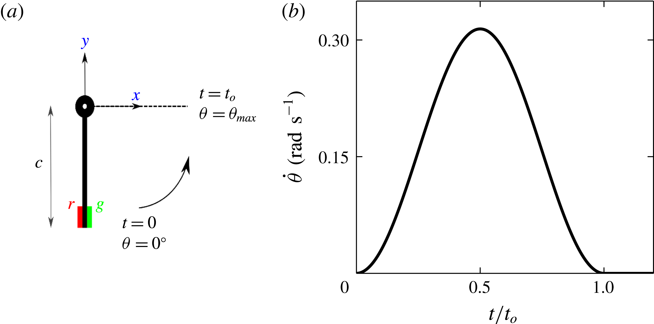
in an otherwise still fluid. A schematic depicting the motion of the plate and a typical angular velocity profile for the plate are shown in figure 1(a) and figure 1(b), respectively. The values of various parameters that describe the motion of the plate are given in § 3.
(a) Schematic describing the plate motion considered in this paper. A thin plate of chord length
 $c$
rotates anti-clockwise about its hinge (set as the origin) from
 $\unicode[STIX]{x1D703}=0^{\circ }$
at
 $t=0$
and stops at
 $\unicode[STIX]{x1D703}=\unicode[STIX]{x1D703}_{max}$
at
 $t=t_{o}$
with a specified angular velocity profile. (b) The angular velocity profile
 $\dot{\unicode[STIX]{x1D703}}$
versus
 $t/t_{o}$
for the flow considered in figure 2 and § 3 with
 $\unicode[STIX]{x1D703}_{max}=90^{\circ }$
and
 $t_{o}=10~\text{s}$
. The red and green patches at the plate tip in (a) show the initial fluorescein and rhodamine dye coating in the dye visualization images shown in figures 2 and 15.

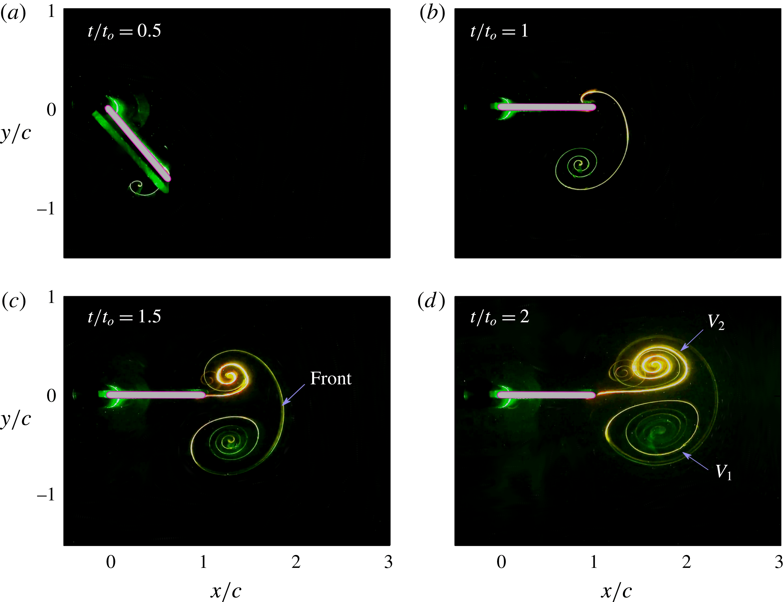
(a–d) Show the images from dye visualization coating experiments at four different times for the flow generated by the plate motion shown in figure 1(b). At
 $t=0$
, the plate tip was coated with green fluorescein and red rhodamine dye on the forward and rearward edges respectively, as shown in figure 1(a). What we refer to as the Front is explicitly marked in (c).
 $V_{1}$
and
 $V_{2}$
in (d) refer to the starting and stopping vortices, respectively. The relatively small vortex-like feature in the background of the stopping vortex in (c,d) is an experimental artefact, possibly due to a combination of an oblique camera viewing angle, weak laser light illumination away from the plane of measurement and free surface reflections.

We describe the basic flow features by presenting the results from a dye visualization experiment in figure 2(a–d). As indicated by the red and green coloured patches at the plate tip in figure 1(a), rhodamine and fluorescein dye were initially coated on the left and right sides. The plate, which is vertical at
 $t=0$
, rotates in the anti-clockwise direction to
 $\unicode[STIX]{x1D703}_{max}=90^{\circ }$
at
 $t=t_{o}$
. A clockwise vortical structure (referred to as the starting vortex
 $V_{1}$
in the rest of this paper), as indicated by the predominantly green spiral formed below the plate at
 $t/t_{o}=0.5$
in figure 2(a), is observed soon after the plate rotation starts. At the instance when the plate rotation stops, the starting vortex is quite prominent, with a distinct curved feature connecting it to the plate (figure 2
b). At
 $t/t_{o}=1.5$
(figure 2
c), we observe the emergence of a separate anti-clockwise vortical structure (referred to as the stopping vortex
 $V_{2}$
in the rest of this paper) that is connected to the starting vortex via what is marked as the Front. At
 $t/t_{o}=2$
(figure 2
d), i.e. well after the plate motion stops, the vortex pair formed by the starting and stopping vortices is seen to move away from the plate in a direction that is nearly aligned with the final plate orientation.
An outstanding question arising from the observations in figure 2 concerns the colours of the dye patterns that appear in the starting and stopping vortices, i.e. what is the spatial origin of the fluid material that get trapped within each of the vortices? Other related fundamental questions include (i) What constitutes the boundaries of the starting and stopping vortices? (ii) What is the kinematic and dynamical significance of the Front? (iii) What is the relation between the vortices and the overall material fluid that gets advected away from the plate? (iv) What is the relation between the linear momentum associated with the overall material fluid that gets advected away from the plate and the forces experienced by the plate and (v) What is the nature of the spirals that occur in the dye visualization images, and how they relate to the spirals reported in previous studies (Pullin & Perry Reference Pullin and Perry1980)? To address the aforementioned questions, we exploit the framework of Lagrangian coherent structures (LCSs), which objectively characterize advective material transport in any fluid flow (Haller Reference Haller2015).
LCSs in any two-dimensional flow are identified as distinct material lines that separate regions of dynamically different fluid material transport. Directly based on various kinds of finite-time coherent behaviour of fluid parcels, LCSs are objective in terms of frame independence and not requiring arbitrary thresholds of quantities such as vorticity magnitude or relative rate of strain (Haller Reference Haller2015). Recent studies (Farazmand, Blazevski & Haller Reference Farazmand, Blazevski and Haller2014) have defined hyperbolic LCSs as locally most attracting or most repelling strainlines; strainlines are curves that are locally orthogonal to the eigenvector associated with the backward-time or forward-time finite-time Lyapunov exponent (bFTLE or fFTLE, respectively). Furthermore, within the framework of LCS, vortices are identified as the region within closed material boundaries where the fluid material advects forward as a coherent unit with no filamentation at the boundaries. These closed boundaries are referred to as elliptic LCSs, which are closed stationary curves of the averaged Lagrangian strain (Haller & Beron-Vera Reference Haller and Beron-Vera2013). LCSs have been shown to be objective descriptions of advective material transport in several flows, with turbulence (Farazmand & Haller Reference Farazmand and Haller2012; Wilson, Tutkun & Cal Reference Wilson, Tutkun and Cal2013) and geophysical applications (Haller & Beron-Vera Reference Haller and Beron-Vera2013) at the forefront. Prior to the strainline-based LCS definition of Farazmand et al. (Reference Farazmand, Blazevski and Haller2014), several studies have used only the FTLE field and associated contours/ridges to study a wide variety of flows. Examples include quasi-two-dimensional turbulence (Mathur et al. Reference Mathur, Haller, Peacock, Ruppert-Felsot and Swinney2007; Kelley, Allshouse & Ouellette Reference Kelley, Allshouse and Ouellette2013), three-dimensional turbulence (Green, Rowley & Haller Reference Green, Rowley and Haller2007; Tang et al. Reference Tang, Mathur, Haller, Hahn and Ruggiero2010) and other vortex-dominated flows (Shadden, Dabiri & Marsden Reference Shadden, Dabiri and Marsden2006; Shadden et al. Reference Shadden, Katija, Rosenfeld, Marsden and Dabiri2007; Cardwell & Mohseni Reference Cardwell and Mohseni2008; Eldredge & Chong Reference Eldredge and Chong2010; Green, Rowley & Smits Reference Green, Rowley and Smits2011; Yang, Jia & Yin Reference Yang, Jia and Yin2012).
The LCS framework has recently been used in the context of fish swimming too. Huhn et al. (Reference Huhn, van Rees, Gazzola, Rossinelli, Haller and Koumoutsakos2015) analysed the velocity field generated numerically by Gazzola et al. (Reference Gazzola, Van, Wim and Koumoutsakos2012), who considered a flexible body whose shape and mid-line kinematics mimicked that of real fish during C-start. The study by Huhn et al. (Reference Huhn, van Rees, Gazzola, Rossinelli, Haller and Koumoutsakos2015) identified elliptic LCSs associated with the shed vortex pairs, and traced them back to the beginning of C-start. They conclude that there are regions outside the elliptic LCSs that advect, along with the shed vortex pairs, with significant linear momentum. These regions outside the elliptic LCSs were not objectively identified by Huhn et al. (Reference Huhn, van Rees, Gazzola, Rossinelli, Haller and Koumoutsakos2015). As we demonstrate in our current study, they are related to regions encompassed within hyperbolic LCSs, which Huhn et al. (Reference Huhn, van Rees, Gazzola, Rossinelli, Haller and Koumoutsakos2015) did not focus on.
It is noteworthy that no previous experimental study has provided a direct experimental demonstration of the relevance of strainline-based hyperbolic (attracting and repelling) and elliptic LCSs in any flow. There have, however, been a few related studies that have shown a correlation between tracer patterns and attracting features in the flow. For example, the experiments of Voth, Haller & Gollub (Reference Voth, Haller and Gollub2002) showed that a passive impurity field has its contours aligned with lines of large stretching in a two-dimensional flow producing chaotic mixing. Visual similarities have been observed between the fluorescence field and bFTLE field in vortex rings too (Olcay & Krueger Reference Olcay and Krueger2008; Shadden Reference Shadden2011). Shadden (Reference Shadden2011) points out that the role of fFTLE is not obvious in flow visualization images. Recently, the ridges in the FTLE field were shown to partly align with the chemiluminescence field associated with the flame in a combustor flow (Sampath, Mathur & Chakravarthy Reference Sampath, Mathur and Chakravarthy2016). In this paper, we present direct experimental evidence, via dye visualization experiments, of the kinematic relevance of attracting and repelling hyperbolic LCSs and elliptic LCSs.
The rest of this paper is organized as follows: § 2 presents a detailed description of the laboratory experiments, numerical simulations and LCS extraction. In § 3, following the validation of our numerical simulations, we show the results based on the LCS extracted from numerically simulated velocity fields. Laboratory experiments that confirm the validity of our results in § 3 are then presented in § 4. We discuss the universality of our results via a parametric study in § 5, followed by our main conclusions and scope for future work in § 6.
2 Methods
In this section, we present the details of the methods adopted in our laboratory experiments, numerical simulations and LCS extraction.
2.1 Laboratory experiments
2.1.1 Set-up
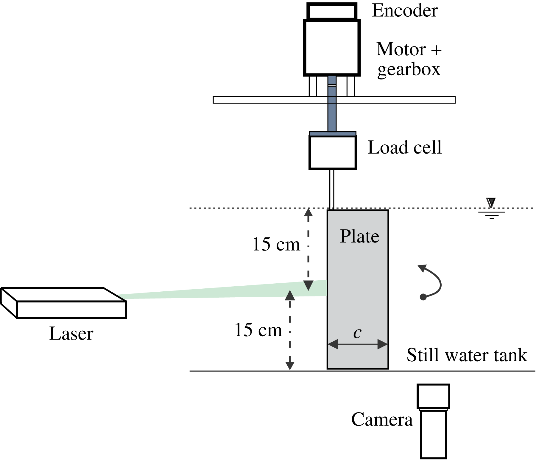
Figure 3 shows a schematic of our experimental set-up, comprising a glass tank of cross-sectional dimensions
 $100\times 70~\text{cm}$
and 45 cm in height. A transparent acrylic plate of span
 $s=300~\text{mm}$
, chord length
 $c=50~\text{mm}$
, thickness 3 mm and with a rounded tip was placed in the still water tank. The plate was sandwich held at the hinge by a 12 mm SS rod that adds stiffness along the span. A transparent false bottom placed 2 mm below the plate gave an effective tank height of
 $H=302~\text{mm}$
. The desired plate motion profile was achieved through a Maxon servo motor plus gearbox arrangement (EC-max30
 $+$
KD32) as shown in figure 3. For the plate speeds involved in our experiments, there were no noticeable vertical movements of the free surface. Further, the Froude number based on the plate velocity
 $c\unicode[STIX]{x1D6FA}_{max}$
and the surface gravity wave speed
 $\sqrt{gH}$
, where
 $g$
is the acceleration due to gravity, is approximately 0.01 in our experiments, indicative of negligible free surface effects. Three different flow measurement techniques, as described below, were employed in our study.
Schematic of the experimental set-up used to obtain the results in figures 2, 4, 5, 12 and 13. The experiments were performed in a water tank of 100 cm length, 70 cm width and 45 cm height. Velocity measurements and dye visualization were performed in a horizontal plane that is 15 cm from the free surface. The 6-axis load cell was used to measure the forces and moments experienced by the plate.

2.1.2 Dye visualization – coating experiments
Using a technique similar to that of Meunier & Leweke (Reference Meunier and Leweke2005), we performed dye visualization coating experiments. A well-mixed dye paste containing a fluorescing agent (either fluorescein or rhodamine) dissolved in a binder (Daler Rowney – Slow Drying Acrylic Medium) and some honey was coated over approximately 1 cm of the span and 3 mm along the chord, around the visualization plane on the plate tip, and then allowed to dry (figure 1). The dye salts that remain bound to the plate surface in stagnant conditions come off the plate once it starts rotating, with the rate of dye release desirably reduced by the presence of honey. A continuous 1 W, 532 nm green laser was used to illuminate the horizontal mid-plane, as shown in figure 3. Colour images were obtained using a Sony Handycam (CX260V) in the HD-Video mode. The dyes used in the coating experiments were heavier than water, as a result of which they sank with time. In this paper, we show the dye visualization images from only those times when the dyes stay within the laser illumination plane.
2.1.3 Dye visualization – injection experiments
Flow visualization experiments were also carried by injecting dye at the beginning of the experiment at pre-determined locations away from the plate surface. The dye was prepared by mixing 10 mg of fluorescein salt with 500 ml of water. A 1 ml syringe, placed outside the tank, with its piston coupled with a long screw, was used to slowly push small amounts of dye. A flexible extension hose connected to the syringe on one end and to a stainless steel hollow pipe (2 mm outer diameter, 1 mm inner diameter) on the other allowed us to choose pre-determined dye injection locations in the mid-plane. The stainless steel pipe and the flexible hosing were slowly withdrawn from the tank before initiating the plate motion. The laser illumination plane in these injection experiments was made relatively thick when compared to the coating experiments. It is noteworthy that a similar dye injection arrangement has been used in the study of DeVoria & Ringuette (Reference DeVoria and Ringuette2012).
2.1.4 Particle image velocimetry (PIV)
PIV measurements were performed to validate our numerical simulations. As shown in figure 3, the horizontal mid-plane spanning
 $200\times 150~\text{mm}$
around the plate was illuminated using a 50 mJ Nd:Yag laser operating at 10 Hz in single pulse mode. A 10-bit 1600 by 1200 pixels Flowsense camera was used to capture images at 10 Hz in synchrony with the laser pulses. PIV processing of the images to obtain the velocity fields on a 100 by 75 Cartesian grid was done with the commercially available Dantec DynamicStudio software. This PIV system has previously been successfully used to study other flows (Murugan & Govardhan Reference Murugan and Govardhan2016). We estimate the overall bias error associated with the PIV processing to be less than 0.01 pixels, which translates to a relative error of around 0.15 % for typical velocities that occur in our experiments.
2.2 Numerical simulations
We performed two-dimensional numerical simulations using the commercial solver FLUENT, which has previously been shown to be accurate in simulating other unsteady flows at Reynolds numbers of approximately 1000. Examples include vortex ring formation by a piston–cylinder arrangement (Shadden et al.
Reference Shadden, Katija, Rosenfeld, Marsden and Dabiri2007), unsteady flow separation induced by a heaving and rotating cylinder (Weldon et al.
Reference Weldon, Peacock, Jacobs, Helu and Haller2008) and flow due to an impulsively started finite plate (Lee et al.
Reference Lee, Hsieh, Chang and Chu2012). Set in laminar mode, the solver simulates the flow in a coordinate frame that moves with the plate, thus allowing us to solve the equations on a stationary mesh. The Navier–Stokes equations are suitably modified to include the additional acceleration terms that appear in a non-inertial coordinate frame. Specifically, the rotating coordinate frame results in the additional terms
 $-2\unicode[STIX]{x1D734}\times \boldsymbol{v}-\unicode[STIX]{x1D734}\times (\unicode[STIX]{x1D734}\times \boldsymbol{r})-(\text{d}\unicode[STIX]{x1D734}/\text{d}t)\times \boldsymbol{r}$
on the right-hand side of the momentum equations (Pedlosky Reference Pedlosky2013). Here,
 $\unicode[STIX]{x1D734}(t)$
is the angular velocity of the rotating frame,
 $\boldsymbol{r}$
and
 $\boldsymbol{v}$
the position vector and the fluid velocity in the rotating frame. The computational domain is chosen to be circular and centred at the plate hinge. The boundary conditions are comprised of no normal flow and no slip on the plate, and an azimuthal velocity on the outer circular boundary that corresponds to stagnant flow conditions in the stationary laboratory frame. The plate was modelled as a thin rectangle with its hinge at the origin, chord length
 $c=0.05~\text{m}$
, thickness to chord ratio
 $0.03$
, with the hinge point and the plate tip rounded with a diameter
 $0.03c$
. The radius of the outer circular boundary of the computational domain was set to be
 $10c$
, which is sufficiently large as the vortex pair generated by the plate motion moves by only approximately
 $5c$
during the period of interest, namely
 $0\leqslant t\leqslant 5t_{o}$
. For the results presented in this paper, a mesh with 85 660 nodes and a time step of 0.002s were used, with the specific values chosen based on grid and time step independence studies. All our numerical simulations were performed for cases with a Reynolds number
 $Re=c^{2}\unicode[STIX]{x1D6FA}_{max}/\unicode[STIX]{x1D708}=785.4$
, where
 $\unicode[STIX]{x1D6FA}_{max}$
is the maximum angular velocity of the plate and
 $\unicode[STIX]{x1D708}=10^{-6}~\text{m}^{2}~\text{s}^{-1}$
is the kinematic viscosity of water. Our numerical simulations are thoroughly validated via comparisons with our experiments and alternate validated numerical solutions, as discussed in § 3.1.
2.3 Lagrangian coherent structures
Hyperbolic and elliptic LCSs in our flow are extracted according to the variational theory described in Haller (Reference Haller2015). The definitions of these LCSs are based on the finite-time Lyapunov exponent
 $\unicode[STIX]{x1D70E}$
(FTLE), defined as (Haller Reference Haller2002)
 $$\begin{eqnarray}\unicode[STIX]{x1D70E}_{t_{o}}^{t_{o}+T}(\boldsymbol{x}_{\boldsymbol{ 0}})=\frac{1}{2|T|}\log \unicode[STIX]{x1D706}_{max}(\unicode[STIX]{x1D71F}),\end{eqnarray}$$
where
 $t_{o}$
and
 $\boldsymbol{x}_{\mathbf{0}}=(x_{0},y_{0})$
are the time and spatial coordinates at which the FTLE field is being evaluated,
 $T$
the integration time and
 $\unicode[STIX]{x1D706}_{max}(\unicode[STIX]{x1D71F})$
denotes the maximum eigenvalue of the matrix
 $\unicode[STIX]{x1D71F}$
(with the corresponding eigenvector denoted by
 $\hat{\unicode[STIX]{x1D709}}$
). The Cauchy–Green deformation tensor,
 $\unicode[STIX]{x1D71F}(\boldsymbol{x}_{\mathbf{0}})$
for a two-dimensional flow is defined as:
 $$\begin{eqnarray}\unicode[STIX]{x1D71F}(\boldsymbol{x}_{\mathbf{0}})=\left[\begin{array}{@{}cc@{}}\displaystyle \frac{\unicode[STIX]{x2202}x(t_{o}+T)}{\unicode[STIX]{x2202}x_{0}} & \displaystyle \frac{\unicode[STIX]{x2202}x(t_{o}+T)}{\unicode[STIX]{x2202}y_{0}}\\ \displaystyle \frac{\unicode[STIX]{x2202}y(t_{o}+T)}{\unicode[STIX]{x2202}x_{0}} & \displaystyle \frac{\unicode[STIX]{x2202}y(t_{o}+T)}{\unicode[STIX]{x2202}y_{0}}\end{array}\right]^{\top }\left[\begin{array}{@{}cc@{}}\displaystyle \frac{\unicode[STIX]{x2202}x(t_{o}+T)}{\unicode[STIX]{x2202}x_{0}} & \displaystyle \frac{\unicode[STIX]{x2202}x(t_{o}+T)}{\unicode[STIX]{x2202}y_{0}}\\ \displaystyle \frac{\unicode[STIX]{x2202}y(t_{o}+T)}{\unicode[STIX]{x2202}x_{0}} & \displaystyle \frac{\unicode[STIX]{x2202}y(t_{o}+T)}{\unicode[STIX]{x2202}y_{0}}\end{array}\right],\end{eqnarray}$$
where the initial tracer positions
 $\boldsymbol{x}_{\mathbf{0}}=(x_{0},y_{0})$
at time
 $t_{o}$
are advected in time according to
 $(\text{d}x/\text{d}t,\text{d}y/\text{d}t)=(u(x,y,t),v(x,y,t))$
to the positions
 $(x(t_{o}+T),y(t_{o}+T))$
at the final time
 $t_{o}+T$
. Numerically,
 $\boldsymbol{x}_{\mathbf{0}}$
is represented using a Cartesian grid with a spatial resolution of 200 points per chord length, and spanning the domain
 $-0.5c\leqslant x_{0}\leqslant 4c$
and
 $-1.5c\leqslant y_{0}\leqslant 1c$
.
 $T>0$
(or
 $T<0$
) corresponds to particle advection in forward (or backward) time, and the corresponding
 $\unicode[STIX]{x1D70E}$
is referred to as fFTLE (or bFTLE). In physical terms,
 $\unicode[STIX]{x1D70E}_{t_{o}}^{t_{o}+T}(\boldsymbol{x}_{\mathbf{0}})$
is a measure of the maximum extent by which infinitesimally close initial conditions around
 $x_{0}$
at
 $t_{o}$
separate during the time interval
 $[t_{o},t_{o}+T]$
. Regions of large magnitudes for fFTLE (bFTLE) are therefore potential regions of significant repulsion (attraction) of neighbouring initial tracer particles in forward time.
Repelling hyperbolic LCSs are defined as distinguished material lines that are locally most repelling in a direction normal to them. In other words, repelling LCSs are everywhere locally orthogonal to the eigenvector
 $\hat{\unicode[STIX]{x1D709}}$
corresponding to
 $\unicode[STIX]{x1D706}_{max}(\unicode[STIX]{x1D71F})$
in the fFTLE field. In this paper, attracting hyperbolic LCSs are identified as repelling LCSs in the corresponding bFTLE field, justified by the notion that normal repulsion in backward time is indicative of normal attraction in forward time. In general, any given blob of fluid gets simultaneously repelled away from and stretched along the repelling and attracting LCSs, respectively during a time interval that is of the order of the integration time
 $T$
. Elliptic LCSs are closed stationary curves of a tangential stretching functional, and are everywhere locally along a vector that is a linear combination of the two eigenvectors of
 $\unicode[STIX]{x1D71F}$
in the fFTLE field (Haller Reference Haller2015). As mentioned in § 1, fluid material inside an elliptic LCS remain as one coherent unit for a finite time
 $T$
with no filamentation at the boundaries.
The numerical implementation of LCS extraction was done using the open source Matlab-based software discussed in Onu, Huhn & Haller (Reference Onu, Huhn and Haller2015). Elliptic LCS extraction requires the specification of a stretching factor
 $\unicode[STIX]{x1D6FD}$
, which is a measure of the change in the arc length of the closed curves. We use the value
 $\unicode[STIX]{x1D6FD}=1$
in all the results presented in this paper. The integration time
 $T$
is in general chosen such that neighbouring initial conditions achieve sufficient separation and hence visibly sharp features emerge in the FTLE fields. In our study, at a given time of interest
 $t$
, we always choose
 $T$
such that
 $t+T=5t_{o}$
for the fFTLE field, and
 $t+T=0$
for the bFTLE field. Our choice of a fixed final time of
 $t+T=5t_{0}$
for the fFTLE calculation ensures that the fluid transport that occurs well after the plate motion stops does not influence our study; it also ensures that the fluid transport that occurs until
 $5t_{0}$
is always accounted for. Furthermore, as discussed in § 3, the flow dynamics relevant for the forces experienced by the plate occurs well inside
 $t/t_{0}\in [0,5]$
. For tracer particle advection, we used the fourth-order Runge–Kutta scheme to integrate in time. Cubic interpolation in space and linear interpolation in time were used to evaluate the fluid velocity at the tracer particle locations.
Throughout this paper, we use the velocity fields from our numerical simulations to perform LCS extraction and analysis. It is also possible to use the experimental PIV measurements to extract the LCSs in the flow. However, since PIV is relatively inaccurate in regions close to the plate, and has a limitation on the spatial extent of the field of view, we use the velocity field from numerical simulations to accurately resolve the LCSs around the plate.
3 Results – LCS from numerical simulations
In this section, we present a detailed analysis of the vortex formation process using the framework of Lagrangian coherent structures for the same case as in figure 2, i.e.
 $\unicode[STIX]{x1D703}_{max}=90^{\circ }$
,
 $t_{o}=10~\text{s}$
, with the Reynolds number being
 $Re=c^{2}\unicode[STIX]{x1D6FA}_{max}/\unicode[STIX]{x1D708}=785.4$
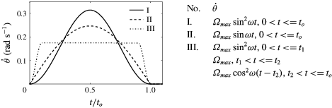
. The plate angular velocity profile is given by
 $\dot{\unicode[STIX]{x1D703}}=\unicode[STIX]{x1D6FA}_{max}\sin ^{2}\unicode[STIX]{x1D714}t$
, where
 $\unicode[STIX]{x1D6FA}_{max}=2\unicode[STIX]{x1D703}_{max}/t_{o}=\unicode[STIX]{x03C0}/10~(\text{rad}~\text{s}^{-1})$
(see figure 1
a,b for a description of the plate motion profile). The
 $\sin ^{2}$
angular velocity profile corresponds to zero acceleration at the starting and stopping times, and at the time of maximum velocity.
3.1 Validation
We start by validating the results from our numerical simulations by comparisons with our experimental measurements and alternate numerical methods. We define the force and moment coefficients as
 $C_{N}=N/[(\unicode[STIX]{x1D70C}(c\unicode[STIX]{x1D6FA}_{max})^{2}sc)/2]$
,
 $C_{A}=A/[(\unicode[STIX]{x1D70C}(c\unicode[STIX]{x1D6FA}_{max})^{2}sc)/2]$
and
 $C_{M}=M/[(\unicode[STIX]{x1D70C}(c\unicode[STIX]{x1D6FA}_{max})^{2}sc^{2})/2]$
, where
 $N,A$
denote the force components normal to and along the plate chord, and
 $M$
the moment about the hinge. Here,
 $\unicode[STIX]{x1D70C}$
is the density of the fluid,
 $c$
and
 $s$
the chord and the span of the plate and
 $\unicode[STIX]{x1D6FA}_{max}$
the maximum angular velocity of the plate. The force components
 $N$
and
 $A$
are obtained by numerically integrating the normal and tangential stresses over the entire plate surface.
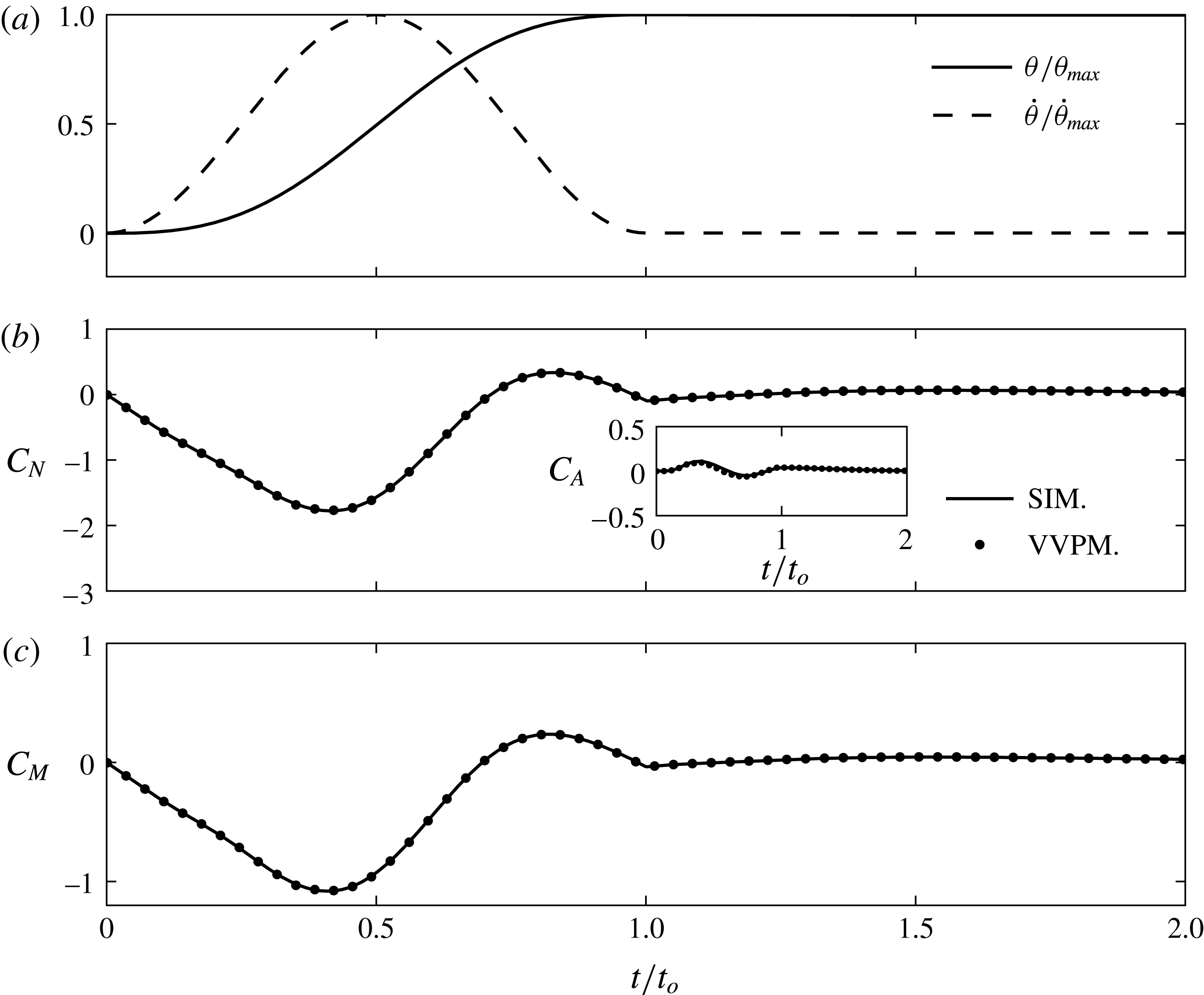
(a) The plate motion profile described in terms of
 $\unicode[STIX]{x1D703}$
versus
 $t$
and
 $\dot{\unicode[STIX]{x1D703}}$
versus
 $t$
for the validation studies presented in § 3.1. (b) The non-dimensional normal and chord-wise force coefficients,
 $C_{N}$
and
 $C_{A}$
(shown in inset), plotted as a function of
 $t/t_{o}$
. The solid line and circle markers correspond to our simulations and viscous vortex particle method (VVPM) simulations (Das, Shukla & Govardhan Reference Das, Shukla and Govardhan2016), respectively, with
 $\unicode[STIX]{x1D703}_{max}=90^{\circ }$
and
 $Re=785.4$
for both the cases. (c) The non-dimensional moment coefficient
 $C_{M}$
plotted as a function of
 $t/t_{o}$
. The line styles correspond to the same scenarios as in (b).

Vorticity field
 $\unicode[STIX]{x1D714}_{z}$
(non-dimensionalized by
 $\unicode[STIX]{x1D6FA}_{max}$
) at
 $t/t_{o}=1$
based on (a) our numerical simulations (SIM.), (b) PIV measurements (EXP.) for the same plate rotation profile as in figure 4(a) with
 $Re=785.4$
. In (a,b) the dashed and the solid lines indicate contours of negative and positive vorticity, respectively. (c) Horizontal velocity profiles from the numerical simulations (——) and the PIV measurements (– – –) across the vertical dotted lines (passing through the respective starting vortex centres) shown in (a,b). (d–f) Same as in figures (a–c), but at time
 $t/t_{0}=2$
with the vertical dotted lines in (d,e) passing through the respective stopping vortex centres.

(a) Trajectories of the position of maximum vorticity magnitude within the starting (bottom trajectories) and stopping (top trajectories) vortex regions from simulations (solid line with closed symbols) and experiments (open symbols) for the same plate motion profile as in figure 4(a) with
 $Re=785.4$
. (b) Corresponding non-dimensional circulation
 $\widehat{\unicode[STIX]{x1D6E4}}$
(
 $=\unicode[STIX]{x1D6E4}/(\unicode[STIX]{x1D6FA}_{max}c^{2})$
) associated with the starting (bottom curves) and stopping (top curves) vortex regions, where
 $\unicode[STIX]{x1D6E4}$
is calculated as the integral of the vorticity over the area encompassed by the contour at 5 % of the peak vorticity magnitude at the respective time. Open and closed symbols correspond to experiments and simulations, respectively. The area integrals of vorticity also included regions around the plate that are not advected away from the plate after the plate motion stops.

In figure 4, we plot the force and moment coefficients as a function of time for the plate motion profile shown in figure 4(a). The Reynolds number for the flow is
 $Re=c^{2}\unicode[STIX]{x1D6FA}_{max}/\unicode[STIX]{x1D708}=785.4$
in both our numerical simulations and the results based on a viscous vortex particle method (VVPM). The VVPM code has previously been used to simulate the flow around a pitching foil in a free stream by Das et al. (Reference Das, Shukla and Govardhan2016). As shown in figure 4(b), the normal force coefficient
 $C_{N}$
from our numerical simulations is in quantitative agreement with the estimate based on VVPM. Similarly, our results also exhibit excellent agreement with VVPM for
 $C_{A}$
(see inset of figure 4
b), which typically is significantly smaller than
 $C_{N}$
for these class of flows. Finally, the moment coefficient
 $C_{M}$
as a function of time (figure 4
c) is also observed to be predicted well by our numerical simulations.
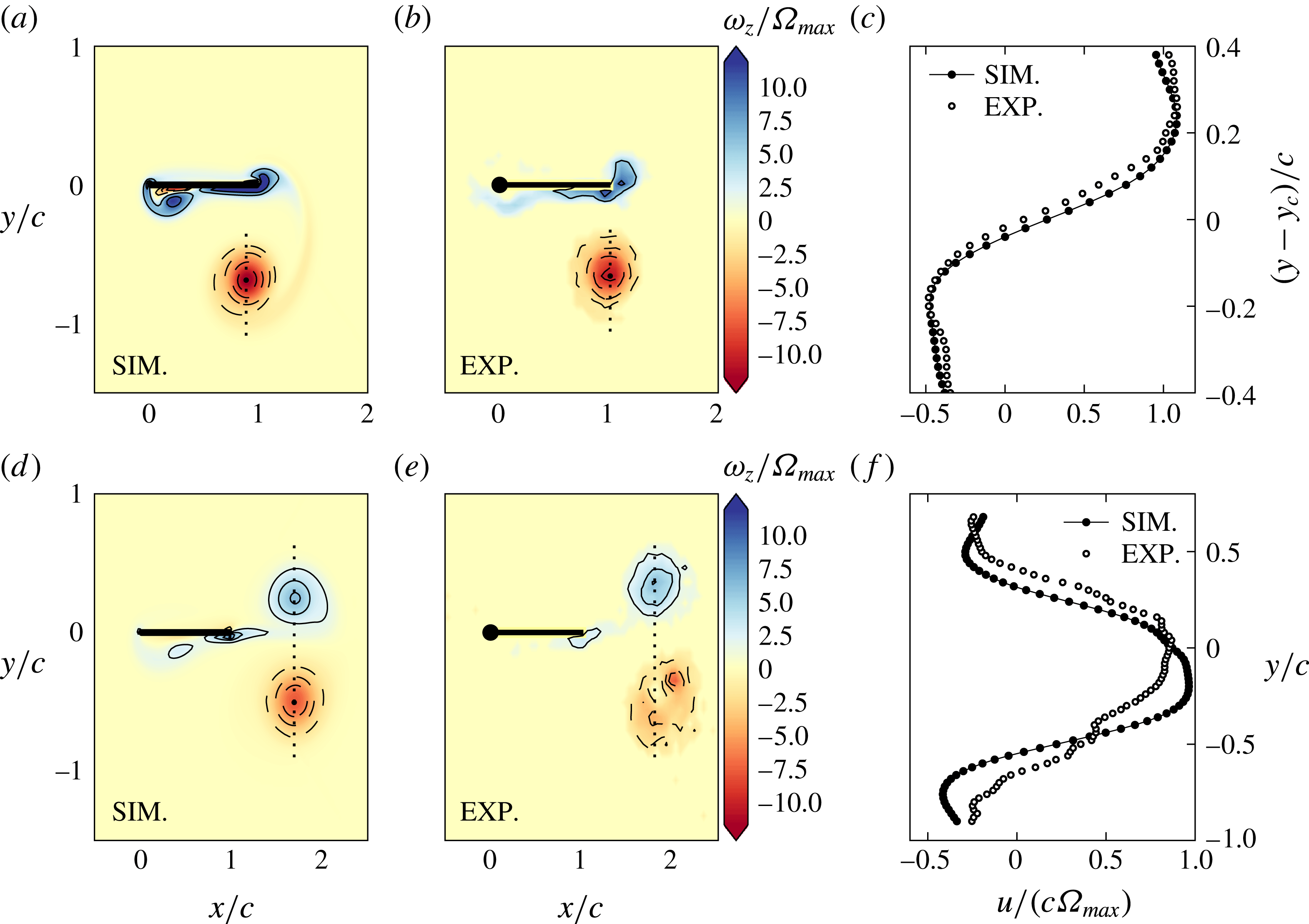
Figure 5(a,b) shows the non-dimensional vorticity field distribution at
 $t/t_{o}=1$
from our numerical simulations and PIV measurements, respectively. Both figures correspond to the plate motion profile shown in figure 4(a) and a Reynolds number of
 $Re=785.4$
. Good qualitative agreement between our numerical simulations and PIV is found, with similar size and strength of the starting vortex in figure 5(a,b). Apart from the starting vortex, there is also a relatively smaller anti-clockwise vortex present right below the plate hinge at
 $t/t_{0}=1$
in our simulations. The formation of this anti-clockwise vortex near the plate hinge is discussed further in § 3.2 and appendix A. The corresponding positive vorticity region below the plate hinge is noticeably weaker in the PIV measurements. The experimental set-up had a 12 mm diameter SS rod holding the plate at the hinge throughout the depth of the tank. In the two-dimensional simulations, however, the plate hinge was modelled as a rounded corner whose diameter was around the plate thickness, i.e. 1.5 mm, thus resulting in the generation of a stronger anti-clockwise vortex below the hinge. Figure 5(c) shows the comparisons in the horizontal velocity profile across the vertical transect shown in figure 5(a,b). There is excellent quantitative agreement in the variation of
 $u$
. The bottom row of figure 5, i.e. figure 5(d–f), show similar comparisons at a later time of
 $t/t_{0}=2$
. While the qualitative nature of the overall vorticity distributions are similar between the simulations and experiments, there are noticeable differences within the starting vortex. The differences may be owing to one or more of the following factors: (i) the errors in the vorticity field arising from numerical differentiation of the velocity field, (ii) the presence of a small background flow in the experiments and (iii) possible three-dimensional effects (Meunier & Leweke Reference Meunier and Leweke2005) that are absent in our simulations. The horizontal velocity profiles across the dotted lines in figure 5(d–e), however, have a similar structure (figure 5
f) with a difference of approximately 11 % in the peak velocity.
For a more detailed comparison between simulations and experiments, we plot the trajectory (
 $t/t_{0}\leqslant 2$
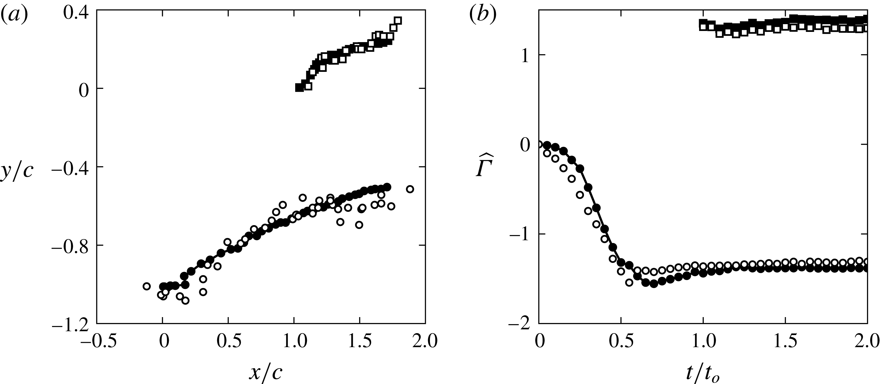
) of the position of peak vorticity in figure 6(a) for the plate motion profile shown in figure 4(a). The starting and stopping vortex trajectories from the experiments and simulations compare favourably with the experimental data for the starting vortex being scattered on both sides of the trajectory from the simulations. We could not perform experimental measurements beyond
 $t/t_{0}=2$
as the vortices started moving out of the camera’s field of view. In figure 6(b), we plot the evolution of the non-dimensional circulation (
 $\widehat{\unicode[STIX]{x1D6E4}}=\unicode[STIX]{x1D6E4}/(\unicode[STIX]{x1D6FA}_{max}c^{2})$
) associated with the starting and stopping vortex regions. The circulation
 $\unicode[STIX]{x1D6E4}$
associated with the vortex regions is calculated as the integral of the vorticity over the area encompassed by the contour at 5 % of the peak vorticity magnitude at the respective time. The area integrals also included the regions in the neighbourhood of the plate that are not necessarily advected away from the plate after the plate motion stops. As shown in figure 6(b), there is excellent quantitative agreement between the simulations and experiments for both the starting and stopping vortex regions, with the difference in the saturation value being around 5 and 8 %, respectively. It is noteworthy that the values at saturation associated with the starting and stopping vortex regions almost cancel each other despite the difference in the strength of the starting and stopping vortices that are advected away from the plate. This is owing to the circulation estimate associated with the stopping vortex region also including the regions around the plate that are not advected away with the vortex pair.
In summary, the data in figures 4–6 demonstrate that our numerical simulations capture the qualitative and quantitative features of the flow with reasonable accuracy. Having established the validity of our numerical simulations, we proceed to use the numerically generated temporally and spatially well-resolved velocity fields to extract the LCSs in the flow.
3.2 Hyperbolic and elliptic LCS
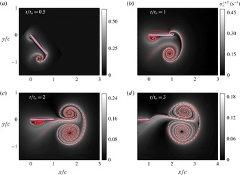
Figure 7(a–d) Show the evolution in time of the bFTLE field,
 $\unicode[STIX]{x1D70E}_{t}^{t+T}$
(in grey scale) computed using an integration time
 $T=-t$
. The attracting hyperbolic LCSs extracted using the method described in § 2.3 are also shown (in red dashed line) in figure 7(a–d). The attracting LCSs in figure 7(b,c) display notable similarity with the dye visualization images shown in figure 2(b,d), including the spiral structures within the vortex pair. While the vortex pair at
 $t/t_{o}=2$
(figure 7
c) appears to be moving along the final plate orientation, it is oriented slightly downwards at
 $t/t_{o}=3$
(figure 7
d). The relative difference in the strengths between the starting and stopping vortices, which causes the vortex pair to deflect downwards, can be attributed to the vorticity associated with (i) the relatively small anti-clockwise vortex a (seen in figure 7
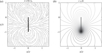
b,c) formed at the hinge/fixed end of the plate, and (ii) the bound circulation around the plate. This anti-clockwise vortex forms as a result of the structure of the flow that is set-up soon after the plate starts moving. As discussed in figure 17 in appendix A, the flow structure at
 $t=0^{+}$
is predicted well by potential flow theory. The anti-clockwise flow around the hinge separates from the plate to result in the formation of the anti-clockwise vortex to the left of the plate hinge. Finally, at
 $t/t_{o}=2,3$
, the Front boundary of the vortex pair seen in figure 2 seems to be correlated with the attracting LCS.
The bFTLE field (shown in grey scale)
 $\unicode[STIX]{x1D70E}_{t}^{t+T}$
with
 $T=-t$
at (a)
 $t=0.5t_{o}$
, (b)
 $t=t_{o}$
, (c)
 $t=2t_{o}$
and (d)
 $t=3t_{o}$
, calculated using the velocity field from our numerical simulations. Shown as dashed red lines in each panel are the corresponding attracting hyperbolic LCSs extracted using the methods described in § 2. The plate rotates about its left tip at
 $(0,0)$
in the anti-clockwise direction during
 $0\leqslant t\leqslant t_{o}$
, with the plate motion profile described in the beginning of § 3 (shown in figure 4
a) corresponding to
 $Re=785.4$
. The plate is shown in hashed pink in all of the panels.

The fFTLE field (shown in grey scale)
 $\unicode[STIX]{x1D70E}_{t}^{t+T}$
with
 $T=5t_{o}-t$
at (a)
 $t=0$
, (b)
 $t=t_{o}$
, (c)
 $t=2t_{o}$
and (d)
 $t=3t_{o}$
, calculated using the velocity field from our numerical simulations. Shown as dashed blue lines are the corresponding repelling hyperbolic LCSs extracted using the methods described in § 2. The plate rotates about its left tip at
 $(0,0)$
in the anti-clockwise direction during
 $0\leqslant t\leqslant t_{o}$
, with the plate motion profile described in the beginning of § 3 (shown in figure 4
a) corresponding to
 $Re=785.4$
. The plate is shown in hashed pink in all of the panels.

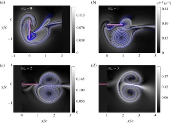
Figure 8 shows the fFTLE field
 $\unicode[STIX]{x1D70E}_{t}^{t+T}$
(in grey scale, computed with an integration time of
 $T=5t_{o}-t$
) and the corresponding repelling hyperbolic LCSs (in blue dashed lines) at times
 $t/t_{o}=0,1,2,3$
. A complex structure is observed for the repelling LCS at
 $t=0$
, with such an extraction of continuous curves being possible as a result of the strainline-based method described in § 2.3. A previous study (Shadden et al.
Reference Shadden, Dabiri and Marsden2006) on the flow generated by a jellyfish used the fFTLE field to identify what is called the upstream wake, thus motivating us to conjecture that the fFTLE field at
 $t=0$
may encompass regions that ultimately end up inside the advected fluid bulk at large times. The validity of this conjecture is discussed later in this section. The repelling LCSs in figure 8(a) demarcate several regions in the neighbourhood of the plate. At
 $t/t_{o}=1$
(figure 8
b), the starting vortex with a spiral structure within is clearly seen in the repelling LCSs, whereas the stopping vortex is just beginning to emerge. While the repelling LCSs are attached to the plate at
 $t/t_{o}=1$
, we observe them to be just detached from the plate at
 $t/t_{o}=2$
(figure 8
c). For larger times, i.e.
 $t/t_{o}=3$
shown in figure 8(d), the repelling LCS contains a distinct boundary that may represent the rear edge of the vortex pair that is shed from the plate.
(a) Elliptic LCSs (solid lines) extracted using the fFTLE field
 $\unicode[STIX]{x1D70E}_{t}^{t+T}$
at
 $t=2t_{o}$
shown in figure 8(c). The green and the pink boundaries correspond to the starting and stopping vortices,
 $V_{1}$
and
 $V_{2}$
respectively. The background colour represents the instantaneous non-dimensionalized vorticity field at
 $t=2t_{o}$
. The elliptic LCSs at
 $t=2t_{o}$
are advected forward in time as material lines to obtain the dashed and dash-dotted curves at
 $t=3t_{o}$
and
 $4t_{o}$
, respectively. (b) Hyperbolic attracting (dashed red) and repelling (dashed blue) LCSs plotted along with the elliptic LCS (solid green and pink) at
 $t/t_{o}=2$
. The region enclosed by the hyperbolic LCSs form the advected bulk that moves away from the plate in a direction close to the final orientation of the plate.

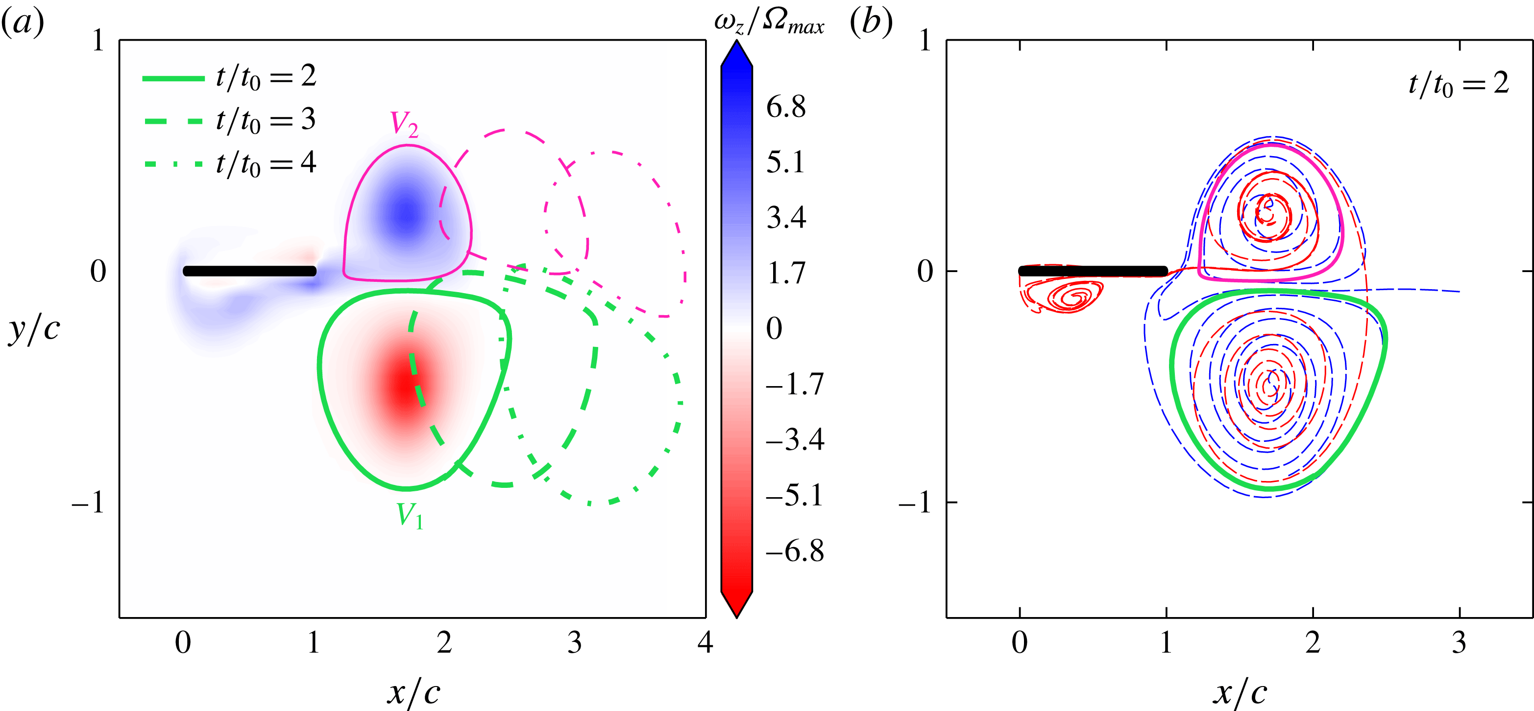
Elliptic LCSs have recently been shown to extract closed boundaries within which the fluid material remains as a coherent unit over a finite period of time, thus resulting in an objective definition of a vortex (Haller & Beron-Vera Reference Haller and Beron-Vera2013). In figure 9(a), we show the elliptic LCSs associated with the starting and stopping vortices at
 $t/t_{o}=2$
, shown as thick green and thin pink solid lines, respectively. Indeed, the advected positions of the elliptic LCSs at later times (
 $t/t_{o}=3,4$
) shown in figure 9(a) imply that the material inside each of these elliptic LCSs advect without any filamentation near the boundaries. These regions within the elliptic LCSs therefore display Lagrangian coherence and remain as coherent blobs of fluid in time. It is also noteworthy that the elliptic LCS boundaries encompass a significantly larger region than what could be defined as a vortex based on a simple thresholding of the vorticity magnitude (shown using the background colour in figure 9
a). We plot the hyperbolic and elliptic LCSs simultaneously at
 $t/t_{o}=2$
in figure 9(b). While the elliptic LCS boundaries seem to overlap with the attracting or repelling LCSs in some regions, there are noticeable regions that are entrapped within the hyperbolic LCSs but lie outside the elliptic LCSs.
In an earlier study by Shadden et al. (Reference Shadden, Katija, Rosenfeld, Marsden and Dabiri2007) on vortex rings, features in the bFTLE and fFTLE fields were used to define vortex boundaries associated with the bulk fluid transport. Extending this approach of Shadden et al. (Reference Shadden, Katija, Rosenfeld, Marsden and Dabiri2007), we construct a region that is bounded everywhere by the locally outermost hyperbolic LCS and investigate the relevance of the region to describe the bulk fluid transport in our flow. Unlike the axisymmetric vortex ring studied in Shadden et al. (Reference Shadden, Katija, Rosenfeld, Marsden and Dabiri2007), the two vortices within the vortex pair of our flow differ in their strengths. As a consequence, the simple scenario of the front and the rear boundaries of the material bulk (that gets transported away from the plate) being given by the attracting and repelling LCSs, respectively, does not hold in our flow. In summary, we have identified the material bulk of the fluid which gets transported away from the plate as the region encompassed by the hyperbolic LCSs; this region will be referred to as the advected bulk in the rest of the paper. A subset of the advected bulk are two separate regions encompassed by elliptic LCS, representing the starting and stopping vortices.
We recall from figure 8 that the repelling LCSs, and possibly the stopping vortex, detach from the plate at around
 $t/t_{o}=2$
. An elliptic LCS extraction at any earlier time would not capture the stopping vortex in its entirety as the stopping vortex completes its formation only around
 $t/t_{o}=2$
. We also note that at a much later time, say
 $t/t_{o}=5$
, the vortex pair will include non-negligible amounts of ambient fluid entrained via diffusion, the influence of which would be insignificant on the flow dynamics at early times. In summary, while the choice of
 $t/t_{o}=2$
for the identification of the advected bulk is not unique, it is probably appropriate for isolating the effects of the plate motion on the vortex pair that is formed. It is also noteworthy that the advected bulk as identified by the hyperbolic LCS boundaries are not too sensitive to the integration time
 $T$
, whereas the elliptic LCS boundaries do depend on the specific choice of
 $T$
. We proceed to investigate the origin and evolution of the various regions within the advected bulk.
(a) Tracer positions at
 $t=0$
obtained by backward advection of material inside the elliptic LCSs (shown in figure 9
a) at
 $t=2t_{o}$
. The green and the pink colours correspond to the starting and stopping vortices, respectively. Shown in grey scale in the background is the fFTLE field
 $\unicode[STIX]{x1D70E}_{t}^{t+T}$
at
 $t=0$
. (b) The lobes at
 $t=0$
that constitute the material inside the hyperbolic LCSs at
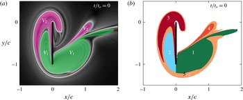
 $t=2t_{o}$
. Lobes 1 (dark green) and 2 (blue) span the entire green region (
 $V_{1}$
) in (a); lobes 3 (red) and 4 (orange) span the entire pink region (
 $V_{2}$
) in (a). Lobe 5 (brown) is obtained by backward advection of the material outside the elliptic LCSs but inside the hyperbolic LCSs at
 $t=2t_{o}$
shown in figure 9(b).

3.3 Advected bulk – where does the fluid come from?
We start by advecting the material inside the elliptic LCSs at
 $t/t_{o}=2$
backward in time to
 $t=0$
. The backward-advected positions of the starting and stopping vortices (
 $V_{1}$
and
 $V_{2}$
) are shown in green and pink, respectively in figure 10(a). Also shown using the background grey scale colour in figure 10(a) is the fFTLE field at
 $t=0$
. There is a strong correlation between the green and pink tracer boundaries, and the ridges in the fFTLE field. There also exist small regions between the tracer boundaries and the fFTLE ridges. In figure 10(b), apart from the backward-advected tracer positions from the starting and stopping vortices, we show as region 5 (in brown) the backward-advected material from the regions outside the elliptic LCSs but within the hyperbolic LCSs at
 $t/t_{o}=2$
. Interestingly, the brown-coloured tracer region in figure 10(b) occupies the small regions between the green/pink tracer boundaries and the fFTLE ridges in figure 10(a). In summary, the fFTLE field of the repelling LCSs at
 $t=0$
provides a direct estimate of the locations of all the fluid material that constitute the advected bulk that eventually forms after the plate motion stops, including an identification of what constitutes the starting and stopping vortices. Motivated by the results from the dye visualization experiment presented in figure 2, we distinguish between the lobes to the forward and rearward sides of the plate: lobes 1 (dark green) and 2 (blue) belong to the starting vortex, and lobes 4 (orange) and 3 (red) belong to the stopping vortex (figure 10
b). The entire brown region in figure 10(b) is referred to as lobe 5.
(a–d) Temporal evolution during
 $0<t\leqslant 3t_{o}$
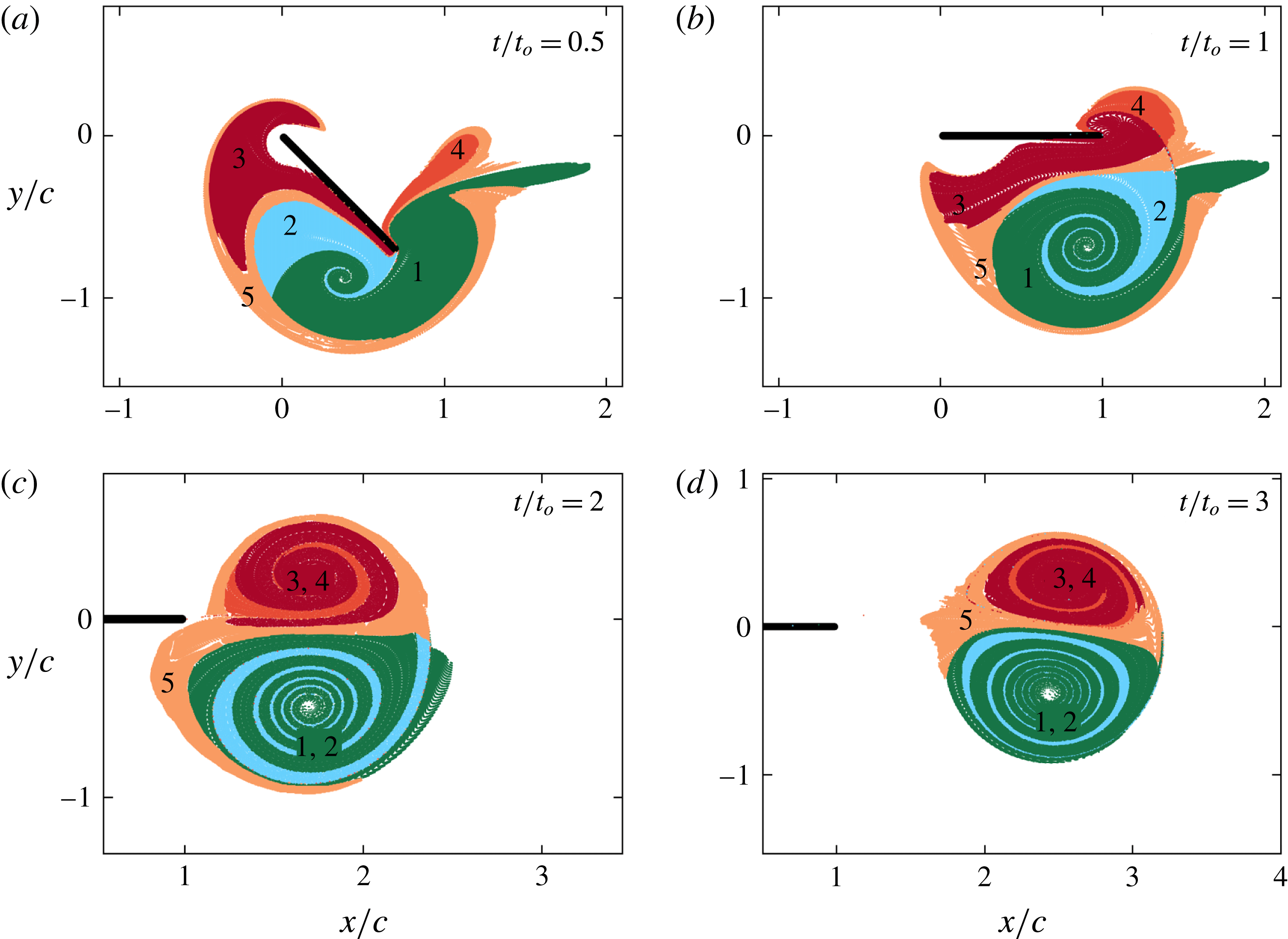
of the material inside the five different lobes of fluid identified in figure 10(b). The times corresponding to each panel is indicated in the top right. Lobes 1 and 2 mix to form the starting vortex. Similarly, lobes 3 and 4 mix to form the stopping vortex. Lobe 5 (brown), which is outside of both the starting and stopping vortices, remains a part of the advected bulk.

Figure 11 shows the evolution of lobes 1–5 with time. Specifically, the advected positions of the material inside various lobes are shown at times
 $t/t_{o}=0.5,1,2,3$
. We recall that, at
 $t/t_{o}=2$
the tracer positions fit in exactly with the boundaries of the hyperbolic and elliptic LCSs shown in figure 9(b). Lobe 1, originally present on the forward side of the plate at
 $t=0$
, crosses over to the rearward side of the plate, also entraining fluid from lobe 2 in the process. At
 $t/t_{o}=2$
(figure 11
c), the fluid from lobe 2 is completely entrained into lobe 1, as a result of which lobe 1 alone is sufficient to describe the elliptic LCS boundary. Interestingly, at
 $t/t_{o}=2$
, the fluid from lobe 2 describes the attracting LCS boundary (figure 9
b) that is present just inside of the front edge of the starting vortex. At a later time, i.e.
 $t/t_{o}=3$
(figure 11
d), the advected attracting and elliptic LCS boundaries at the front edge of the starting vortex become coincidental. We also quantify the areas contained in lobes 1 and 2 (denoted by
 $A_{lobe1}$
and
 $A_{lobe2}$
) of the starting vortex
 $V_{1}$
by defining the entrainment fraction
 $\unicode[STIX]{x1D702}_{V1}=A_{lobe2}/(A_{lobe1}+A_{lobe2})$
, which takes a value of 26 %. We have thus precisely estimated the amount of fluid material from either side of the plate at
 $t=0$
that ultimately constitutes the starting vortex.
We recall from figure 1 that the starting vortex
 $V_{1}$
is mostly green in an experiment in which the forward and rearward sides of the plate were coated green and red, respectively. This observation is understood via the results in figure 11 where lobe 1 is clearly seen to be in contact with the forward side of the plate at
 $t/t_{o}=0.5$
whereas lobe 2 is prevented from touching the rearward side of the plate by the material from lobe 3 in between. At
 $t=0$
(figure 10
b) too, while lobe 1 (dark green) is in contact with the forward side of the plate tip, a thin filament from lobe 3 is present in between lobe 2 and the rearward side of the plate tip. While the dye visualization experiment shown in figure 1 is inconclusive about the relative amounts of fluid from either side of the plate that get into the starting vortex, our LCS analysis has conclusively identified the initial locations of all the fluid material that gets entrapped in the starting vortex.
Lobes 3 and 4, which constitute the stopping vortex, exhibit an evolution in time that is similar to that of lobes 1 and 2 of the starting vortex, but with the main difference of entrainment (of lobe 4 by lobe 3) occurring after the plate motion stops. Lobe 3, which is originally on the rearward side of the plate, acquires sufficient momentum during the plate motion to move towards the forward side and subsequently entrain the fluid in lobe 4. Also, since lobe 3 is much more in contact with the plate than lobe 4 (figures 10
b, 11
a,b), the dye visualization experiment in figure 1 produced a predominantly red-coloured stopping vortex. For
 $t/t_{o}\geqslant 2$
, lobe 3 alone describes the elliptic LCS boundary associated with the stopping vortex, with lobe 4 being fully entrained into it. The entrainment fraction for the stopping vortex
 $V_{2}$
, defined as
 $\unicode[STIX]{x1D702}_{V2}=A_{lobe4}/(A_{lobe3}+A_{lobe4})$
, takes a value of 18 %.
Lobe 5, which corresponds to the fluid that is present outside of the elliptic LCSs but inside of the hyperbolic LCSs at
 $t/t_{o}=2$
, never comes in contact with the plate and wraps around the stopping vortex as the flow evolves in time. For
 $t/t_{o}\geqslant 2$
, lobes 1 and 2 and lobes 3 and 4 move as individual coherent elliptic units, whereas lobe 5 gets significantly stretched and folded while still remaining a part of the advected bulk. It is worthwhile repeating that the delineations between the five different lobes are captured accurately by the repelling LCS at
 $t=0$
.
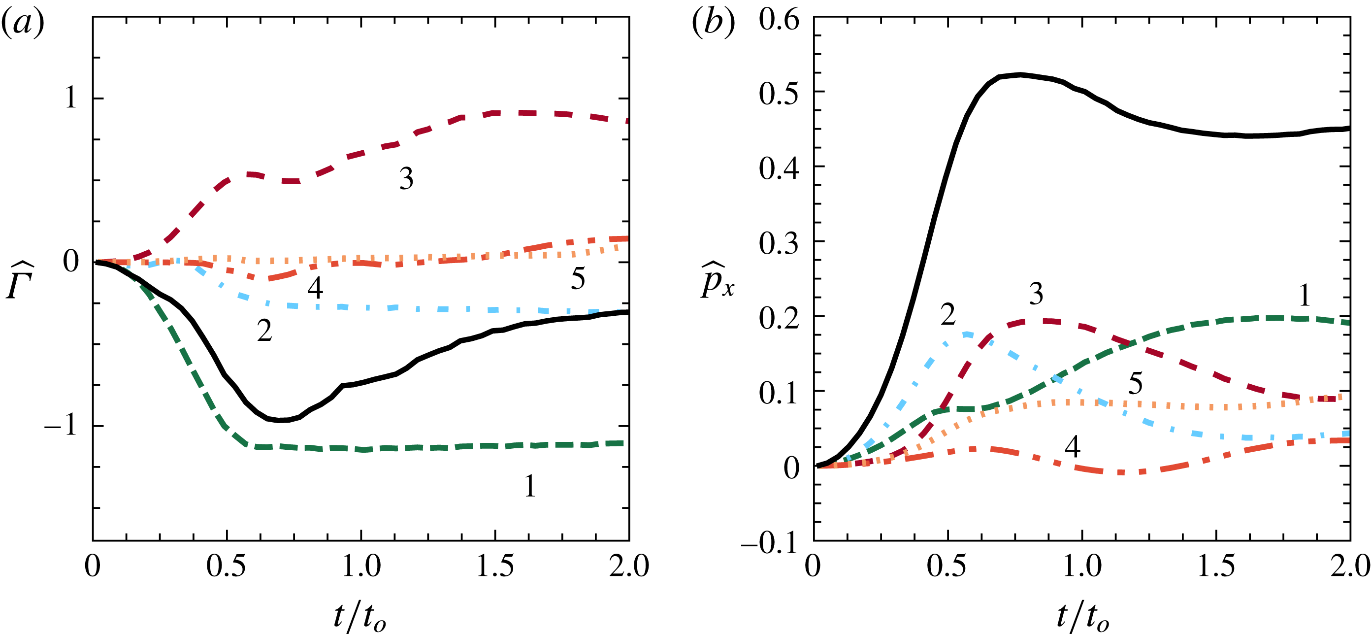
(a) Temporal evolution of the non-dimensional circulation
 $\widehat{\unicode[STIX]{x1D6E4}}=\unicode[STIX]{x1D6E4}/(c^{2}\unicode[STIX]{x1D6FA}_{max})$
associated with each of the five different lobes of fluid identified in figure 10(b), where
 $\unicode[STIX]{x1D6E4}=\int \unicode[STIX]{x1D714}_{z}\,\text{d}A$
. (b) Corresponding non-dimensional horizontal momentum
 $\widehat{p_{x}}$
associated with the five lobes of fluid and the entire advected bulk, where
 $\widehat{p_{x}}=p_{x}/(\unicode[STIX]{x1D70C}\unicode[STIX]{x1D6FA}_{max}c^{3})$
and
 $p_{x}=\int \unicode[STIX]{x1D70C}u\,\text{d}A$
. The colours of the curves in both (a) and (b) are consistent with those in figure 10(b) and the lobe numbers are marked near the curves. The solid black curves in (a,b) show the total circulation and the horizontal momentum associated with the entire advected bulk.

We define the non-dimensional circulation associated with a given lobe as
 $\widehat{\unicode[STIX]{x1D6E4}}=\int \unicode[STIX]{x1D714}_{z}\,\text{d}A/(c^{2}\unicode[STIX]{x1D6FA}_{max})$
, where
 $\unicode[STIX]{x1D714}_{z}$
is the vorticity and the integral is over the entire area occupied by the lobe. Owing to the discretized representation of a lobe, which actually is a continuous region of material fluid, the calculation of
 $\widehat{\unicode[STIX]{x1D6E4}}$
is non-trivial, particularly if the lobe stretches or folds significantly in its evolution. Here,
 $\widehat{\unicode[STIX]{x1D6E4}}$
at a given time is numerically estimated by binning an area that encompasses all the tracer particles associated with a lobe, and then identifying those bins that contain at least one tracer particle. The area integral of vorticity associated with the lobe is then performed over these identified bins. The size of the bins and the density of tracer particles were chosen such that the numerical estimate is accurate for pre-defined areas with known circulation values. More details of the numerical procedure used to calculate
 $\widehat{\unicode[STIX]{x1D6E4}}$
for each lobe is given in appendix B. In figure 12(a), we plot the evolution of
 $\widehat{\unicode[STIX]{x1D6E4}}$
associated with each of the lobes 1–5. Lobe 1 acquires negative circulation right from
 $t=0$
, and saturates at a nearly constant value of
 $-$
1.2 at
 $t/t_{o}=0.6$
. In other words, lobe 1 continuously acquires negative circulation during the entire acceleration phase of the plate motion (
 $0\leqslant t/t_{0}\leqslant 0.5$
) and some time soon after (
 $0.5\leqslant t/t_{0}\leqslant 0.6$
), and acquires no further significant circulation during the remaining plate deceleration phase. It is also noteworthy that lobe 1 loses contact with the plate at some point in the interval
 $0.5<t/t_{0}<0.6$
, paving way for lobe 3 in the stopping vortex to gain additional circulation during the plate deceleration phase. These results build upon previous related studies (Kim & Gharib Reference Kim and Gharib2011; DeVoria & Ringuette Reference DeVoria and Ringuette2013b
) where the relation between the stopping vortex formation and the plate deceleration phase was investigated. The circulation associated with lobe 2 remains negligible till
 $t/t_{o}\sim 0.3$
and then increases during the interval
 $0.3<t/t_{o}<0.6$
before saturating at a value of
 $-$
0.33. While lobe 1 acquires its vorticity from being in contact with the forward side of the plate right from
 $t=0$
and subsequently separates off the plate tip, lobe 2 acquires its vorticity only during entrainment by lobe 1. We recall from figure 11 that lobe 2 makes minimal contact with the plate and hence has only lobe 1 as its potential source of vorticity. The small value of the time scale (
 ${\approx}0.3t_{o}$
) over which lobe 2 acquires vorticity suggests that the intricate spiral structure inside the starting vortex significantly enhances the rate of vorticity mixing by creating additional interfacial area over which lobes 1 and 2 are in contact.
Lobe 3, which belongs to the stopping vortex, acquires vorticity right from the beginning as a result of being in contact with a significant portion of the rearward side of the plate. It is noteworthy that the stopping vortex, while appearing to emerge only after
 $t/t_{o}=1$
in the dye visualization experiment shown in figure 1, actually acquires vorticity right from
 $t=0$
. Then, at around
 $t/t_{o}=0.7$
, lobe 3 separates from the plate tip and hence gains additional vorticity before saturating at a value of 1 at
 $t/t_{o}=1.5$
. Lobe 4 attains negligible vorticity during
 $t/t_{o}<0.5$
before acquiring negative vorticity by being on the forward side of the plate. At
 $t/t_{o}=0.65$
, lobe 4 begins to get entrained by lobe 3 and hence acquires positive vorticity to reach a value of 0.15 at
 $t/t_{o}=2$
. Lobe 5, though being a part of the advected bulk, acquires negligible vorticity throughout. Finally, the circulation associated with the entire advected bulk (black solid curve in figure 12
a) increases in magnitude as the starting vortex forms, and then starts decreasing even before the plate motion stops.
To investigate the dynamical relevance of the various lobes in the advected bulk, we calculate the linear momentum (
 $\boldsymbol{p}=\int \unicode[STIX]{x1D70C}\boldsymbol{u}\,\text{d}A$
) associated with each of them. The numerical procedure used to calculate
 $\boldsymbol{p}$
is the same as that used for
 $\widehat{\unicode[STIX]{x1D6E4}}$
, as detailed in appendix B. We recall from our discussion in § 1 that turning manoeuvres result in the fish moving along its final orientation, which is along the
 $x$
-axis in our studies. Furthermore, we have shown that the generated vortex pair moves roughly along the direction of the final plate orientation. We therefore restrict our dynamical relevance studies to the horizontal momentum
 $p_{x}$
only. In figure 12(b), we plot the temporal evolution of non-dimensional horizontal momentum,
 $\widehat{p_{x}}$
defined as
 $\widehat{p_{x}}=p_{x}/(\unicode[STIX]{x1D70C}\unicode[STIX]{x1D6FA}_{max}c^{3})$
for each of lobes 1–5 and the sum total associated with the entire advected bulk. Lobes 1 and 2 start acquiring horizontal momentum right from
 $t=0$
, with lobe 2 gaining
 $\widehat{p_{x}}$
faster. Lobe 2, which gets entrained by lobe 1 to form the starting vortex, attains maximum
 $\widehat{p_{x}}$
at around
 $t/t_{0}=0.55$
, after which its horizontal momentum decays to a small value (
 ${\approx}0.05$
) at
 $t/t_{0}=2$
. Lobe 1 acquires
 $\widehat{p_{x}}$
faster after
 $t/t_{0}=0.5$
before saturating at a value of around
 $\widehat{p_{x}}=0.2$
at
 $t/t_{0}=2$
. Lobes 3 and 4 start acquiring horizontal momentum at around
 $t/t_{0}=0.3$
, with lobe 4 possessing a small negative
 $\widehat{p_{x}}$
at
 $t/t_{0}=1$
. Lobe 3 attains a maximum
 $\widehat{p_{x}}$
of around 0.2 at
 $t/t_{0}=0.8$
. At
 $t/t_{0}=2$
,
 $\widehat{p_{x}}$
for lobe 3 flattens at around 0.09, whereas lobe 4 settles at around
 $\widehat{p_{x}}=0.04$
, nearly the same as lobe 2.
Strikingly, lobe 5, while being outside of the elliptic LCSs, acquires significant horizontal momentum, settling at a value of around
 $\widehat{p_{x}}=0.09$
at
 $t/t_{0}=2$
. Furthermore, lobe 5 acquires its almost steady horizontal momentum as early as
 $t/t_{0}=0.7$
, and contributes to 20 % of the horizontal momentum associated with the entire advected bulk at
 $t/t_{0}=2$
. It is therefore important that the region encompassed by the hyperbolic LCSs, which includes the elliptic LCSs and lobe 5, is considered to identify the advected bulk. Finally, the total horizontal momentum of the entire advected bulk (solid line in figure 12
b) is observed to attain a maximum value of
 $\widehat{p_{x}}=0.55$
at
 $t/t_{0}=0.8$
before reaching an almost steady value of
 $\widehat{p_{x}}=0.46$
at
 $t/t_{0}=1.5$
.
(a) Temporal evolution of the total horizontal impulse (
 $I_{x}(t)=\int _{0}^{t}F_{x}\,\text{d}t$
, where
 $F_{x}$
is the
 $x$
-component of the instantaneous force experienced by the plate) experienced by the plate (solid curve) and the horizontal momentum associated with the entire advected bulk (
 $p_{x1-5}$
, dashed curve). (b) Temporal evolution of the ratio
 $p_{x1-5}/I_{x}$
. In (b), the ratio for times
 $t/t_{0}<0.1$
is not shown as
 $I_{x}$
is very small for
 $t/t_{0}<0.1$
.

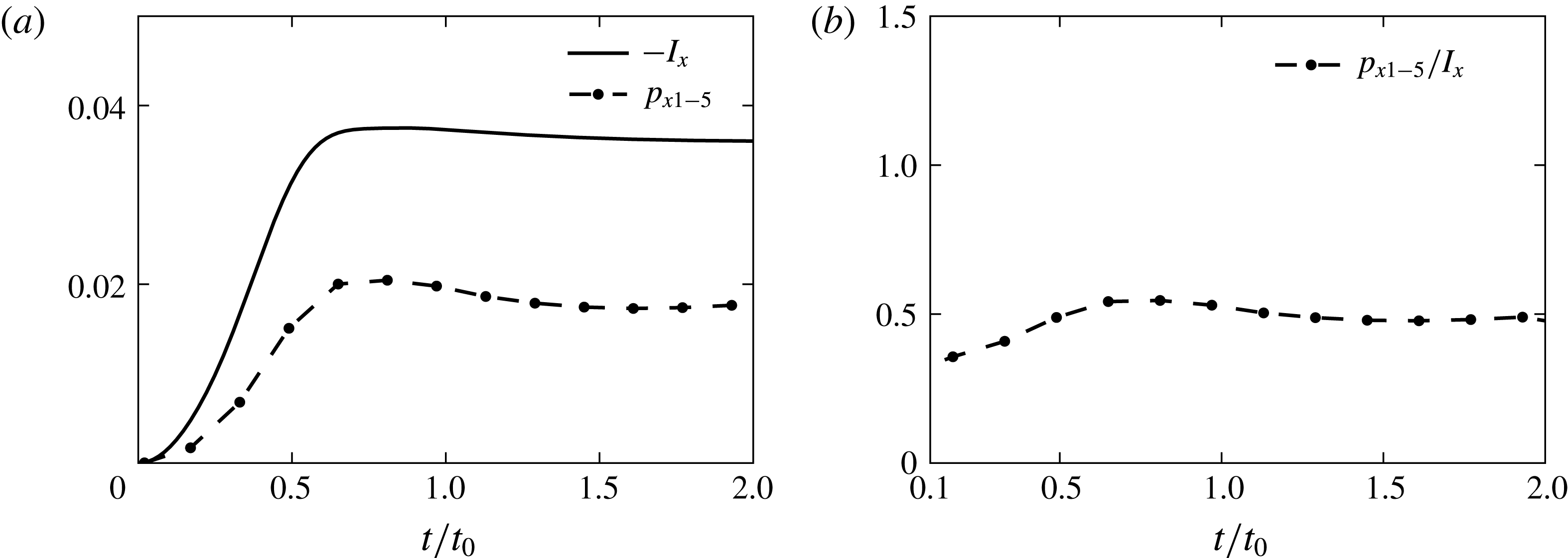
We proceed to investigate the relation between the horizontal momentum associated with the advected bulk and the total horizontal impulse felt by the plate. As shown by the solid curve in figure 13(a), the plate experiences significant horizontal force till around
 $t/t_{0}=0.8$
, before the total impulse (calculated as
 $I_{x}(t)=\int _{0}^{t}F_{x}\,\text{d}t$
, where
 $F_{x}$
is the horizontal force estimated from numerical simulations) saturates at around
 $I_{x}=0.035$
. The evolution of
 $p_{x}$
associated with the entire advected bulk (dashed line) follows a similar trend as that of
 $I_{x}$
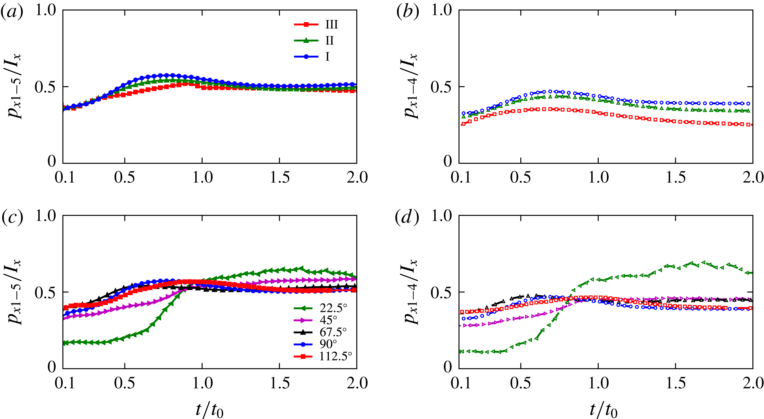
, suggesting that the advected bulk contains a constant fraction of the total impulse experienced by the plate. Indeed, as shown in figure 13(b), the ratio
 $p_{x1-5}/I_{x}$
is reasonably steady at a value of around
 $0.5$
for the entire duration of
 $0.1\leqslant t/t_{0}\leqslant 2$
. Furthermore, based on a control volume analysis, one can argue that
 $I_{x}$
is equal to the horizontal momentum associated with the entire flow around the plate (Epps Reference Epps2010).
The steady value of
 $p_{x1-5}/I_{x}$
of around 0.5 for
 $t/t_{0}>1$
can be partly understood in terms of how the overall fluid momentum is distributed between the advected bulk and the rest of the flow. The advected bulk is bound by the hyperbolic LCSs, which can be approximated as material lines in the flow (Peng & Dabiri Reference Peng and Dabiri2007; Haller Reference Haller2011) on which no normal flow is possible. One can therefore model the rest of the flow as a potential flow created by a bluff body whose size, shape and momentum are the same as that of the advected bulk. As seen in figure 11, the entire advected bulk can be reasonably represented by an equivalent deformed elliptical shape, whose aspect ratio is close to unity at both
 $t/t_{0}=2$
and
 $t/t_{0}=3$
. For an ellipse of major and minor axes
 $2a$
and
 $2b$
moving along its major axis, the added mass coefficient associated with its direction of motion is given by
 $\unicode[STIX]{x1D70C}\unicode[STIX]{x03C0}b^{2}$
, where
 $\unicode[STIX]{x1D70C}$
is the fluid density (Batchelor Reference Batchelor2000). Thus, the overall horizontal momentum of the potential flow around the ellipse moving along
 $x$
with a velocity
 $U$
is given by
 $\unicode[STIX]{x1D70C}\unicode[STIX]{x03C0}b^{2}U$
. Since the ellipse models the advected bulk filled with the fluid of density
 $\unicode[STIX]{x1D70C}$
, its horizontal momentum is
 $\unicode[STIX]{x1D70C}\unicode[STIX]{x03C0}abU$
. The ratio between the horizontal momentum of the ellipse and the overall horizontal momentum of the flow (ellipse plus the potential flow around it) is therefore
 $r=1/(1+b/a)$
. For a circular shape, i.e.
 $a=b$
,
 $r=0.5$
, which is very close to the value we observe for
 $p_{x1-5}/I_{x}$
at
 $t/t_{0}=2$
in figure 13(b). For a relatively wide range of
 $0.75\leqslant (b/a)\leqslant 1.25$
,
 $r$
varies from 0.57 to 0.44, suggesting that the ratio
 $p_{x1-5}/I_{x}$
may remain close to 0.5 as long as the aspect ratio of the advected bulk is around unity, and does not depend too strongly on either the size or the momentum imparted to the advected bulk. It is important to note that the advected bulk at
 $t/t_{0}=1$
(figure 11
b) is far from being idealized as an elliptic shape of aspect ratio close to unity; the relevance of our physical arguments pertaining to added mass is therefore unclear for times closer to
 $t/t_{0}=1$
. Finally, it is worthwhile to note that the simple model of dividing the entire flow into what occurs inside the advected bulk and the potential flow around it is possible only via the identification of the advected bulk by hyperbolic LCSs, which encompass one continuously connected coherent region of fluid.
4 Results – visualizing LCS in laboratory experiments
In this section, we present results from laboratory dye visualization experiments to validate our numerical results in § 3. Our study represents the first efforts to provide direct experimental evidence for the relevance of elliptic and hyperbolic LCSs in any flow. The only other direct experimental visualization of LCS-like features was performed by Voth et al. (Reference Voth, Haller and Gollub2002), who showed alignment between contours of a passive impurity field and lines of large stretching in a two-dimensional flow with periodic forcing.
4.1 Repelling LCSs at
 $t=0$

Here, we show results from dye visualization injection experiments that were designed to directly demonstrate the relevance of the five different lobes of fluid identified at
 $t=0$
in § 3. Specifically, we release dye in different regions of the flow and verify if the tracer evolution is consistent with the LCSs predicted based on the numerical simulations. To recall our results from figure 10(b) in § 3, lobes 1 (dark green) and 2 (blue) belong to the starting vortex, whereas lobes 3 (red) and 4 (orange) belong to the stopping vortex. Lobe 5 (brown), while being outside the starting and stopping vortices, still is a part of the advected bulk. In figure 14, each row corresponds to a different experiment. In all the figures in the first column (corresponding to
 $t=0$
in each experiment) of figure 14, lobes 1–5 at
 $t=0$
identified using numerical simulations is superimposed on the experimentally acquired image.
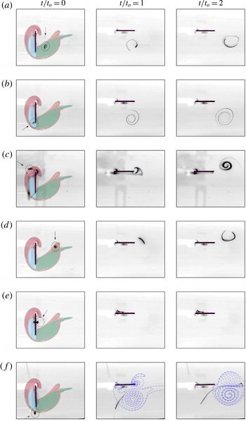
Experimental visualization of the temporal evolution of dye (shown in black) released in (a) lobe 1 (dark green), (b) lobe 2 (blue), (c) lobe 3 (red), (d) lobe 4 (orange), (e) outside the advected bulk and (f) on the boundary dividing lobe 5 (brown) and the region outside the advected bulk. In each row, the dye visualization is shown at
 $t=0$
,
 $t=t_{o}$
and
 $t=2t_{o}$
in columns 1, 2 and 3, respectively. Lobes 1–5 identified at
 $t=0$
using numerical simulations are superimposed on all the
 $t=0$
images with the same colour scheme as in figure 10(b). Circles around the initial dye location (and arrows pointing to them) are drawn in the
 $t=0$
images to serve as a visual aid. For the
 $t=t_{o}$
and
 $t=2t_{o}$
images in the last row, the repelling LCS at the corresponding times are shown in blue.

As shown in figure 14(a), the dye was carefully released within lobe 1 in the experiment corresponding to figure 14(a). Indeed, at
 $t/t_{o}=1$
and
 $t/t_{o}=2$
, the dye is observed to be present entirely within the starting vortex which moves away from the plate after the plate motion stops. Similarly, figure 14(b) demonstrates that the dye released within lobe 2 is also contained within the starting vortex at later times. Figure 14(c,d) provides corresponding experimental evidence for the dye released in both lobes 3 and 4 ending up in the stopping vortex. In figure 14(e), at
 $t=0$
, we released the dye on the forward side of the plate where none of the five lobes are present. As shown in the second and third columns in figure 14(e), the dye does not enter the advected bulk and instead remains (without any significant stretching or folding) in the neighbourhood of the plate even at
 $t/t_{o}=2$
. Finally, in figure 14(f), we released a patch of dye on the repelling LCS boundary at
 $t=0$
, thus being partly inside lobe 5 and partly outside the advected bulk. The normal repulsion of the repelling LCS boundary to the left of the starting vortex is directly evident in the second and third panel in figure 14(f) (where the repelling LCS are shown in blue dashed lines), with the portion of the dye outside the advected bulk getting left behind. The portion of the dye inside lobe 5 (brown region) gets significantly stretched and occupies the region in between the starting and stopping vortices, which is fully consistent with our conclusions in § 3. To the best of our knowledge, figure 14(f) represents the first ever experimental evidence for the normal repulsion characteristic of repelling LCSs in any flow.
In summary, figure 14 has provided detailed experimental evidence for the kinematic relevance of each of lobes 1–5 at
 $t=0$
in determining the tracer patterns in the flow at later times. We highlight here that we have performed several dye visualization experiments other than what are shown in figure 14. While the placement of the dye patch at desired locations was a challenge owing to small background flow that was present before the plate motion starts, the subsequent evolution of the dye patch for
 $t>0$
was always consistent with what the LCS analysis predicts for the initial location of the dye at the instance when the plate motion starts. It is intriguing that despite differences being present between the experiments and simulations (§ 3.1), the five different lobes in the experiment are very accurately captured by the LCS calculations based on the numerical velocity fields. This is, however, consistent with an earlier study by Haller (Reference Haller2002) that showed that hyperbolic LCSs in model velocity fields containing noise can be reliable predictors for the LCSs in the corresponding true velocity fields.
4.2 Attracting LCS
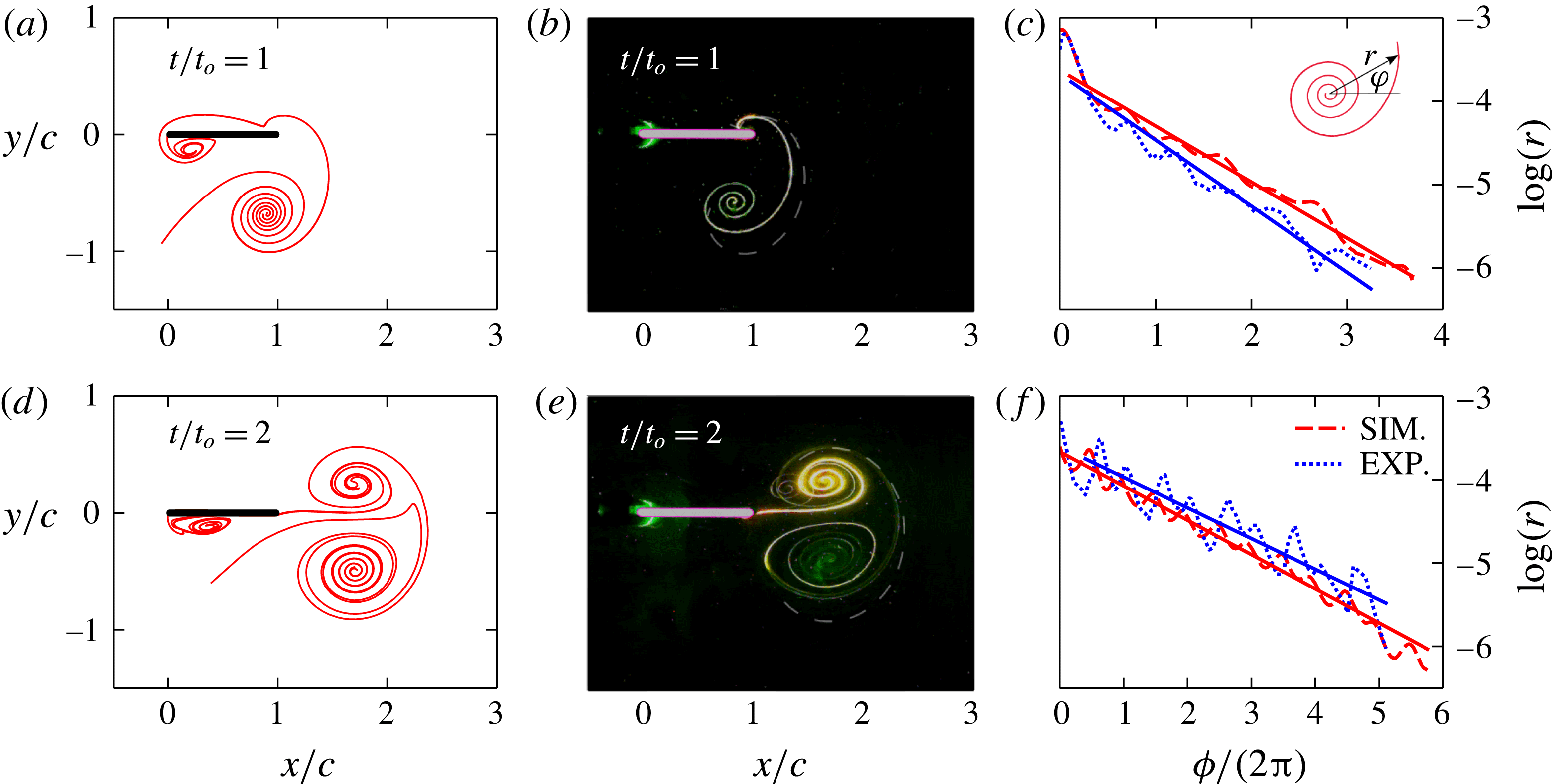
In this section, we present a direct comparison between the tracer patterns observed in dye visualization coating experiments shown in figure 1 and the attracting LCS (shown in figure 7) at the corresponding times. Figure 15(a,d) shows the attracting LCS at
 $t/t_{o}=1,2$
, with the corresponding dye visualization coating images shown in figure 15(b,e). There is striking qualitative similarity between the tracer patterns and the attracting LCS, including the intricate spiral structure (connected to the Front) within the starting and stopping vortices, at both
 $t/t_{o}=1$
and 2. The similarities between the dye visualization images and the attracting LCS are understood in terms of the kinematic properties of the attracting LCS. An initial blob of passive tracers tends to move towards and then stretches along neighbouring attracting LCSs (Voth et al.
Reference Voth, Haller and Gollub2002; Mathur et al.
Reference Mathur, Haller, Peacock, Ruppert-Felsot and Swinney2007), thus resulting in the blob eventually marking attracting LCSs. These results represent the first experimental study to demonstrate the relevance of strainline-based attracting LCSs in describing tracer advection, which is directly visualized without any numerical effort. It is noteworthy that earlier LCS extraction algorithms based on either FTLE thresholding (Shadden et al.
Reference Shadden, Dabiri and Marsden2006) or ridge extraction (Mathur et al.
Reference Mathur, Haller, Peacock, Ruppert-Felsot and Swinney2007) are not capable of resolving the spirals inside the vortices as continuous curves, thus reaffirming the benefits of a strainline-based approach.
(a) Attracting LCS at
 $t=t_{o}$
based on numerical simulations (same as in figure 7
b), (b) image obtained at
 $t=t_{o}$
in the dye coating experiment (same as in figure 2
b) with the front portion of the attracting LCS in (a) shown as the white dashed line, (c) the variation of
 $\log (r)$
with
 $\unicode[STIX]{x1D719}$
associated with the spiral (connected to the Front) inside the starting vortex. Dashed and dash-dotted lines in (c) correspond to numerically obtained attracting LCS and experimental dye coating image, respectively, at
 $t=t_{o}$
. The definition of
 $r$
and
 $\unicode[STIX]{x1D719}$
is shown in the inset of (c). (d–f) Same as (a–c) but at the later time of
 $t=2t_{o}$
. The slopes of the best-fit straight lines in (c) are
 $-$
0.67 and
 $-$
0.8, respectively for the attracting LCS and the dye coating experiment. The corresponding values for (f) are
 $-$
0.41 and
 $-$
0.37.

In figure 15(b,e) we also plot the front attracting LCS boundary on top of the dye visualization images. While the point of intersection between the tracer boundary and the plate agrees well with that of the attracting LCS boundary, there is noticeable difference between the tracer boundary and the attracting LCS away from the plate. Possible reasons for this discrepancy include errors associated with the calibration of the camera, the effects of the small background flow that is present in the tank, and small differences in the plate motion profile (especially at the beginning and the end when the plate velocities are small) between the simulations and the experiments. The camera calibration errors emerge from the spatially non-uniform distortion of the image, and the camera’s line of view not being exactly orthogonal to the laser illumination plane. The agreement between the attracting LCS boundary and the Front edge presented by the dye is relatively better at a later time, i.e.
 $t/t_{o}=2$
as shown in figure 15(e). Finally, we infer that the Front boundary from dye coating experiments can be used as an approximate estimate for the front edge of the advected bulk if detailed velocity field measurements are not available. Furthermore, if we assume that the starting and stopping vortices are of similar size and strength, a reflection of the Front boundary about the axis passing through the vortex centres can be used to construct the back boundary of the advected bulk too, as suggested by Olcay & Krueger (Reference Olcay and Krueger2008) for a piston-generated symmetric vortex ring.
We now proceed to characterize the spiral structure within the starting vortex in more detail. As shown in the inset of figure 15(c), we define a
 $r-\unicode[STIX]{x1D719}$
coordinate system, with the origin for
 $\unicode[STIX]{x1D719}$
located on the outer boundary of the spiral structure in the starting vortex. Plotted in figure 15(c,f) are the variation of
 $\log (r)$
with
 $\unicode[STIX]{x1D719}/2\unicode[STIX]{x03C0}$
at
 $t/t_{o}=1$
and 2. The red dashed curves are based on the attracting LCSs obtained using numerical simulations, and the blue dotted curves correspond to the dye patterns in the dye visualization coating experiments. The
 $r$
versus
 $\unicode[STIX]{x1D719}$
variation is observed to be well represented by a exponential fit at both times, i.e.
 $r\sim \text{e}^{m(\unicode[STIX]{x1D719}/2\unicode[STIX]{x03C0})}$
, with the estimates for
 $m$
based on numerical simulations and dye visualization experiments being in reasonable quantitative agreement. Specifically, as indicated in the caption of figure 15, the values of
 $m$
from the experiment and the simulation differ by approximately 16 and 10 % at
 $t/t_{0}=1$
and
 $t/t_{0}=2$
, respectively. Interestingly, the logarithmic nature of the spiral structure within vortices seems to be prevalent in other systems as well, as reported by Everson & Sreenivasan (Reference Everson and Sreenivasan1992) for dye visualizations in turbulent jets, Kelvin–Helmholtz instabilities and vortex rings. In summary, we conclude that attracting LCSs represent objective counterparts to patterns that are observed in dye visualization experiments in any flow. Furthermore, LCSs may represent a useful complementary tool to characterize spiral structures inside vortices in general (Moffatt Reference Moffatt1993; Lepage, Leweke & Verga Reference Lepage, Leweke and Verga2005), and subsequently address questions related to passive tracer and vorticity mixing within them (Meunier & Villermaux Reference Meunier and Villermaux2003).
5 Results – parametric study
In §§ 3 and 4, we presented a detailed LCS analysis and corresponding experiments for the specific plate motion profile given by
 $\dot{\unicode[STIX]{x1D703}}=\unicode[STIX]{x1D6FA}_{max}\sin ^{2}\unicode[STIX]{x1D714}t$
with
 $\unicode[STIX]{x1D703}_{max}=90^{\circ }$
and
 $t_{o}=10~\text{s}$
, corresponding to a Reynolds number value of
 $Re=785.4$
. In this section, we investigate if the main results of § 3 extend to other plate motion profiles. Specifically, we consider three different profiles, as shown in table 1. Profile I describes the plate motion considered in § 3, whereas profile II corresponds to a sinusoidal variation in time for
 $\dot{\unicode[STIX]{x1D703}}$
and thus has non-zero acceleration at
 $t=0$
and
 $t=t_{o}$
. Profile III is a significant change from profiles I and II, with a constant angular velocity for most of the time and large angular acceleration for small periods of time at the beginning and the end. The plate motion stops at the same time
 $t_{o}$
for all of the profiles, and
 $\unicode[STIX]{x1D6FA}_{max}$
for each profile chosen such that
 $\unicode[STIX]{x1D703}_{max}=90^{\circ }$
. The value of
 $\unicode[STIX]{x1D6FA}_{max}$
decreases as we go from profile I to profile III.
Functional forms of
 $\dot{\unicode[STIX]{x1D703}}$
versus
 $t$
for the three plate motion profile shapes considered in § 5.
 $\unicode[STIX]{x1D6FA}_{max}$
and
 $\unicode[STIX]{x1D714}$
are given by: (i)
 $\unicode[STIX]{x1D6FA}_{max}=2\unicode[STIX]{x1D703}_{max}/t_{o}$
,
 $\unicode[STIX]{x1D714}=\unicode[STIX]{x03C0}/t_{0}$
(profile I), (ii)
 $\unicode[STIX]{x1D6FA}_{max}=\unicode[STIX]{x03C0}\unicode[STIX]{x1D703}_{max}/2t_{o}$
,
 $\unicode[STIX]{x1D714}=\unicode[STIX]{x03C0}/t_{0}$
(profile II), (iii)
 $\unicode[STIX]{x1D6FA}_{max}=\unicode[STIX]{x1D703}_{max}/(0.5t_{1}+t_{2}-t_{1}+0.5(t_{o}-t_{2}))$
,
 $\unicode[STIX]{x1D714}=\unicode[STIX]{x03C0}/2t_{1}$
,
 $t_{1}=0.1t_{o}$
,
 $t_{2}=0.9t_{o}$
(profile III).

We perform the same LCS analysis as in § 3 for all three profiles shown in table 1, and thus identify the various regions of the fluid at
 $t=0$
that end up in the advected bulk at
 $t/t_{o}=2$
. We also investigate the effects of varying
 $\unicode[STIX]{x1D703}_{max}$
for the plate motion described by profile I. As shown in appendix C, all the cases we consider show that five different lobes of fluid at
 $t=0$
, with the same kinematic characteristics as for the case presented in § 3, eventually form the advected bulk after the plate motion stops. A detailed characterization of these five lobes in terms of the relative areas they occupy, and their spatial structure is also presented in appendix C.
Temporal evolution of (a)
 $p_{x1-5}/I_{x}$
, the normalized horizontal momentum associated with the entire advected bulk, (b)
 $p_{x1-4}$
, the horizontal momentum associated with lobes 1–4 for the three cases presented in figure 18(a–c). Temporal evolution of (c)
 $p_{x1-5}$
, the horizontal momentum associated with the entire advected bulk, (d)
 $p_{x1-4}/I_{x}$
, the normalized horizontal momentum associated with lobes 1–4 for various
 $\unicode[STIX]{x1D703}_{max}$
for the plate motion profile I, including the cases shown in figure 18(d–f). The total impulse
 $I_{x}$
imparted to the plate is calculated as
 $I_{x}(t)=\int _{0}^{t}F_{x}(t)\,\text{d}t$
, where
 $F_{x}(t)$
is the instantaneous horizontal force experienced by the plate. The horizontal direction, i.e.
 $x$
-axis (see figure 1), represents the final plate orientation for all the cases presented in this figure.

To investigate the universality of our conclusion in § 3 that the horizontal momentum in the advected bulk for
 $t/t_{0}>1$
accounts for roughly half the total impulse experienced by the plate, we plot the temporal evolution of
 $p_{x1-5}/I_{x}$
for all the cases considered in figure 19. For the three different profiles presented in figure 18(a–c), the temporal evolution of
 $p_{x1-5}/I_{x}$
is almost identical, with all three of the curves settling very close to a value of 0.5 for
 $t/t_{0}>1$
(figure 16
a). For various
 $\unicode[STIX]{x1D703}_{max}$
(all corresponding to the same plate motion profile I), while the curves differ at small times, they again flatten out at around 0.5 for
 $t/t_{0}>1$
(figure 16
c). To demonstrate the importance of including lobe 5 in the advected bulk, we plot the temporal evolution of
 $p_{x1-4}/I_{x}$
in figure 16(b,d). While the steady state values of the ratio is noticeably below 0.5, the closeness between the various curves also reduces (in comparison to figure 16
a,c) when lobe 5 is not included in the calculations. In summary, across all the cases we studied in this paper, it seems reasonable to conclude that the advected bulk, including lobes 1–5, after the plate motion stops contains around half the total impulse imparted to the plate.
With regards to turning manoeuvres in fish, our study has shown that the advected bulk ultimately moves in a direction closely aligned with the final plate orientation. This is consistent with the well-established observation of fish moving in a direction aligned with its final orientation during their turning manoeuvres (Weihs Reference Weihs1972). Also, the advected bulk seems to account for around half the total impulse imparted to the fish during the turning manoeuvre. Furthermore, we have built on previous studies (Gazzola et al. Reference Gazzola, Van, Wim and Koumoutsakos2012; Huhn et al. Reference Huhn, van Rees, Gazzola, Rossinelli, Haller and Koumoutsakos2015) to establish LCS as a potentially significant tool to understand various kinematic and dynamical aspects of turning manoeuvres and C-start, including the role of the tail motion profile and its flexibility in determining the nature of the generated vortical flow and the total impulse imparted to the fish. LCSs may also prove to be useful in the design and control of underwater vehicles that mimic fish manoeuvres.
6 Discussion and conclusions
In this paper, we have performed a kinematic analysis of an idealized model of the propulsive stroke in the turning manoeuvre of fish. The study investigates the two-dimensional, incompressible flow that results from a finite rotation about the hinge of an infinitesimally thin rigid plate in still fluid. Numerical simulations at Reynolds numbers of the order of 1000, which were validated using comparisons with experimental velocity measurements and alternate numerical simulations, were used to generate temporally and spatially well-resolved velocity fields. Lagrangian coherent structures (LCSs), which delineate dynamically distinct regions in a given flow, were then extracted using recently developed variational theory (Haller Reference Haller2015). The attracting hyperbolic LCSs were shown to describe the tracer patterns that result from dye visualization experiments performed by coating dye on both sides of the plate tip. The region encompassed by the attracting and repelling hyperbolic LCSs were then shown to objectively identify the material bulk of the fluid that gets advected away from the plate after the plate motion stops, in a direction almost aligned with the final plate orientation. Elliptic LCSs, which were used to define the boundaries of the starting and stopping vortices, are contained within the advected bulk with non-negligible amounts of fluid outside the elliptic LCSs but inside the advected bulk.
The fluid material within the advected bulk was then traced back to the initial time (
 $t=0$
) when the plate motion starts. Motivated by the dye visualization coating experiments, we then defined five different lobes of fluid that eventually form the advected bulk. These five different lobes are captured well by the repelling hyperbolic LCS boundaries at
 $t=0$
. Of these five lobes of fluid at
 $t=0$
, lobes 1 and 2 form the starting vortex, lobes 3 and 4 the stopping vortex, with lobe 5 forming the rest of the advected bulk, thus completely describing the kinematic origin of the advected bulk. The temporal evolution of the five lobes of fluid showed that lobe 1, which is initially in contact with the plate on the right side, entrains lobe 2, which is never in contact with the plate, to form the starting vortex. Similarly, lobe 3, which is initially in contact with a significant portion of the plate on the left side, entrains lobe 4 to form the stopping vortex. The temporal evolution of the circulation associated with each of the lobes then showed that lobe 1 and 3 attain significant circulation from the plate right from
 $t=0$
, whereas lobes 2 and 4 attain circulation only upon getting entrained by lobes 1 and 3, respectively. Lobe 5, which lies outside the elliptic LCSs, but inside the advected bulk, attains negligible circulation at all times though it represents approximately one third of the advected bulk area.
The temporal evolution of the horizontal momentum contained within each of lobes 1–5 showed that lobe 5 accounts, on an average across all the plate motion profiles we study, for approximately 25 % of the horizontal momentum of the entire advected bulk. After the plate motion stops (final plate orientation is horizontal across all the cases we studied), the horizontal momentum of the advected bulk was shown to be around half of the total impulse experienced by the plate from
 $t=0$
. The advected bulk accounting for half the total impulse imparted to the plate was physically interpreted by dividing the entire flow into the advected bulk region and a potential flow that gets set-up around it if the advected bulk region is thought of as a moving bluff body.
We then performed novel dye visualization laboratory experiments to directly demonstrate that fluid material from lobes 1 and 2 indeed form the starting vortex, lobes 3 and 4 the stopping vortex, and lobe 5 the rest of the advected bulk. We also showed that dye released outside of the five lobes of fluid at
 $t=0$
get left behind outside the advected bulk at later times. Dye visualization coating experiments were then understood in terms of the attracting LCS, which were also shown to be objective counterparts to tracer patterns to describe the spiral structure inside the starting vortex. To the best of our knowledge, this study represents the first experimental demonstration of the kinematic relevance of attracting and repelling hyperbolic LCSs and elliptic LCSs in any flow set-up in controlled laboratory settings.
The repelling LCS at
 $t=0$
, which depict the five lobes of fluid that form the advected bulk were then shown to be qualitatively similar for a range of plate motion profiles. The advected bulk area is related to both the area swept by the plate and the extent to which the initial five lobes of fluid wrapped around the immediate neighbourhood of the plate. The entrainment ratios associated with the starting and stopping vortices, quantified by the area of the entrained lobe relative to the total area of the corresponding vortex, are found to be always around 0.25 for all the plate motion profiles that correspond to a Reynolds number of approximately
 $785$
. It was then shown that the linear momentum of the advected bulk region accounted for around half the total impulse experienced by the plate in the direction of its final orientation across all the plate motion profiles we studied. Thus, apart from experimentally demonstrating the kinematic relevance of LCSs, we have also shown that LCSs have dynamical significance in an idealized model of the propulsive stroke of the turning manoeuvre in fish.
In general, if one is interested only in identifying the advected bulk that has a bearing on the forces experienced by the plate, it is sufficient to calculate the hyperbolic LCSs alone. The advected bulk, identified using the hyperbolic LCSs, is unique, objective and represents a single coherent material volume. The calculation of elliptic LCSs, however, has other important implications: (i) elliptic LCSs objectively delineate the advected bulk region into regions associated with the starting and stopping vortices, and the rest; hyperbolic LCSs alone cannot achieve this delineation, (ii) our study also shows that elliptic LCSs alone cannot be used to identify the advected bulk. Specifically, the result of a constant ratio (of 0.5) between the linear momentum of the advected bulk and the total impulse experienced by the plate is not valid if one were to use the elliptic LCSs alone to identify the advected bulk.
In the future, it would be worthwhile to identify the motion profiles associated with the tail in the turning manoeuvre of real fish. The inclusion of plate flexibility, the presence of a forebody, three-dimensionality and the preparatory stroke of the turning manoeuvre are required to make the current study even more relevant for the real world. Finally, it is important to recognize that the current study does not incorporate the effects of the kinematic response of the fish to the forces that result from the flow generated by it. The inclusion of a free stream could potentially make the study relevant for other scenarios such as moving fish or underwater vehicles.
Acknowledgements
The authors thank A. Das for his help in providing data from viscous vortex particle methods for our validation studies, and Nithiyaraj for his help with the dye visualization injection experiments. The inputs from P. Meunier on the dye visualization coating experiments is acknowledged. We also thank G. Jacobs for his inputs on using Fluent in the rotating frame coordinates. We thank the three anonymous referees for their insightful comments and suggestions. M.M. acknowledges funding from Indian Space Research Organisation under the project number ASE1415163ISROMANK.
Appendix A. Potential flow
Figure 17(a) shows the streamlines at
 $t/t_{o}=0.1$
obtained using numerical simulations for the case described in § 3. To understand this flow pattern at early times, we compute the streamfunction based on the potential flow theory at
 $t=0$
. The complex potential, obtained by imposing the no normal flow boundary condition at the plate and no flow far from the plate, at
 $t=0$
is given by
 $w(\unicode[STIX]{x1D709})=-0.25j\unicode[STIX]{x1D6FA}(1/\unicode[STIX]{x1D709}^{2}+4/\unicode[STIX]{x1D709})$
, where
 $j=\sqrt{-1}$
,
 $\unicode[STIX]{x1D6FA}$
the instantaneous angular velocity of the plate, and
 $\unicode[STIX]{x1D709}=x+yj$
the spatial coordinate of any point in the domain (Sarpkaya Reference Sarpkaya1966). As shown in figure 17(b), the flow pattern based on potential flow theory indeed accurately describes the flow pattern at early times in the numerical simulations. As the plate starts rotating anti-clockwise about its hinge at the origin, the fluid in the vicinity of the plate tip moves in the clockwise direction around the plate tip. In contrast, the fluid around the hinge tends to turn around the hinge in the anti-clockwise direction. The dividing streamline between the clockwise and anti-clockwise fluid motions intersects the plate at around 0.6
 $c$
from the hinge. Similar arguments have previously been used to gain insights into the flow patterns at early times in other unsteady flows (Lighthill Reference Lighthill1986).
(a) Streamlines at
 $t/t_{o}=0.1$
obtained from numerical simulations for the case discussed in § 3, (b) corresponding streamlines based on potential flow theory at
 $t=0$
.

Appendix B. Numerical calculation of circulation and momentum
To numerically calculate the temporal evolution of circulation and linear momentum associated with a given lobe of fluid which may filament at small spatial scales as it evolves, we initiate tracer particles with a uniform grid resolution
 $r_{p}$
within the lobe at
 $t=0$
. Upon advection according to the local velocity field, these tracers lose their uniform distribution within the lobe. At a given time
 $t$
, to calculate
 $\int _{lobe}\unicode[STIX]{x1D714}_{z}\,\text{d}A$
and
 $\int _{lobe}\unicode[STIX]{x1D70C}u\,\text{d}A$
associated with the lobe, a rectangular bounding box is drawn and gridded with bins of size
 $r_{g}\times r_{g}$
. The area integral of the relevant quantity (vorticity or velocity) over the lobe is then estimated as a summation of the integrals over those bins that contain at least one tracer particle. The integral over individual bins is estimated as the interpolated value of the relevant quantity at the bin centre multiplied by its area. In our calculations, we fixed
 $r_{p}$
at a value of
 $c/250$
, and varied
 $r_{g}$
till the numerical procedure was deemed accurate for the entire starting vortex at
 $t/t_{0}=2$
. The starting vortex, identified using elliptic LCS, at
 $t/t_{0}=2$
is bounded by a simple closed boundary, and hence a direct calculation of the area integral of
 $\unicode[STIX]{x1D714}_{z}$
or
 $\unicode[STIX]{x1D70C}u$
is possible, thus generating a reference value with which the accuracy of our numerical procedure can be quantified. We note that, for a given
 $r_{p}$
, decreasing
 $r_{g}$
need not always reduce the error in the numerical estimate of the area integrals. Reducing
 $r_{g}$
below an optimum value, in fact, artificially reduces the area associated with the tracer particles, thus requiring us to identify the optimum
 $r_{g}$
for a given plate motion profile and a fixed
 $r_{p}$
.
Table showing the values and errors associated with the calculation of the non-dimensional circulation of the starting vortex,
 $\widehat{\unicode[STIX]{x1D6E4}_{V1}}$
at time
 $t/t_{0}=2$
for varying bin size
 $r_{g}$
. The
 $\widehat{\unicode[STIX]{x1D6E4}_{V1}}$
is calculated for the case presented in § 3 for varying
 $r_{g}$
. The estimate of circulation calculated by doing
 $\int _{V1}\unicode[STIX]{x1D714}_{z}\,\text{d}A$
over the area occupied by the starting vortex given by the elliptic LCS at
 $t/t0=2$
is
 $-$
2.76 and this value is used to estimate the errors involved calculating
 $\widehat{\unicode[STIX]{x1D6E4}_{V1}}$
using the numerical procedure discussed in this section.
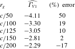
In table 2, we show the variation of the estimated circulation associated with the starting vortex at
 $t/t_{0}=2$
as a function of
 $r_{g}$
in our numerical procedure. We find that
 $r_{g}=c/150$
corresponds to the smallest error, and hence proceed to use
 $r_{p}=c/250$
and
 $r_{g}=c/150$
for all the five lobes of fluid for the plate motion profile associated with table 2. We repeat the same procedure of identifying the value of
 $r_{g}$
that results in accurate estimates of total circulation for the starting vortex at
 $t/t_{0}=2$
for other plate motion profiles we study. We note that the value of
 $r_{g}$
that results in the most accurate estimates of total circulation or linear momentum may vary for various lobes. To verify the robustness of our conclusions based on the circulation and momentum evolution of lobes 1–5, we calculated the corresponding temporal evolution curves for three different values of
 $r_{g}$
,
 $c/100$
,
 $c/125$
and
 $c/150$
. The three different curves are within 5 % of each other until
 $t/t_{0}=1$
, with a maximum difference of around 10 % occurring at
 $t/t_{0}=2$
. Furthermore, the overall trends of circulation/momentum evolution associated with individual lobes were observed to be insensitive to the specific value of
 $r_{g}$
in the range
 $c/150\leqslant r_{g}\leqslant c/100$
. In the future, it would be worthwhile to design more accurate numerical algorithms to estimate circulation or momentum associated with material volumes that stretch or fold significantly.
Appendix C. Parametric study – areas and entrainment fractions
In this section, we present the details of the advected bulk and the associated five lobes of fluid for three different plate motion profiles (see table 1) and various stopping angles
 $\unicode[STIX]{x1D703}_{max}$
. Figure 18(a–c) shows the initial regions of fluid that end up in the starting vortex (green), stopping vortex (pink) and the rest of the advected bulk (brown) at
 $t/t_{o}=2$
for profiles I, II and III with
 $\unicode[STIX]{x1D703}_{max}=90^{\circ }$
. Also shown in the background colour in figure 18(a–c) is the fFTLE field at
 $t=0$
. The spatial structures of the five different lobes at
 $t=0$
are qualitatively similar for all the three plate motion profiles, with the area associated with the brown region noticeably increasing from profile I to profile III.
In figure 18(d–f), we show the five different lobes at
 $t=0$
for profile I with
 $\unicode[STIX]{x1D703}_{max}=45^{\circ },67.5^{\circ },112.5^{\circ }$
, respectively. Again, the spatial structures of the lobes are all qualitatively similar, with the lobe areas being larger for larger
 $\unicode[STIX]{x1D703}_{max}$
. Interestingly, for small
 $\unicode[STIX]{x1D703}_{max}$
, lobe 3 (belonging to the stopping vortex) is present only to the left of the plate and does not wrap around the plate hinge as it does for
 $\unicode[STIX]{x1D703}_{max}=67.5^{\circ },90^{\circ },112.5^{\circ }$
. While the lobes are mostly in contact with the entire left side of the plate for all
 $\unicode[STIX]{x1D703}_{max}$
shown, the extent of the plate on its right side over which the lobes are in a close neighbourhood increases as
 $\unicode[STIX]{x1D703}_{max}$
increases.
The five different lobes of fluid at
 $t=0$
that constitute the advected bulk for (a–c) profiles I–III with
 $\unicode[STIX]{x1D703}_{max}=90^{\circ }$
, (d–f) profile I with
 $\unicode[STIX]{x1D703}_{max}=45^{\circ },67.5^{\circ },112.5^{\circ }$
. The Reynolds number associated with each figure is (a)
 $Re=785.4$
, (b)
 $Re=616.9$
, (c)
 $Re=436.3$
, (d–f)
 $Re=785.4$
. In all the figures, lobes 1 and 2 form the starting vortex, 3 and 4 the stopping vortex and 5 the rest of the advected bulk. The fFTLE field at
 $t=0$
is also shown in grey scale in all the plots.

(a) The non-dimensional areas associated with the advected bulk (●; black), the starting vortex (▴), the stopping vortex (▸) and the rest of the advected bulk (▪; ginger) for the three cases presented in figure 18(a–c); (b) the corresponding entrainment fractions associated with the starting (●; bondiblue) and stopping vortices (▪; cadmiumorange). (c,d) The non-dimensional lobe areas and the entrainment ratios plotted as a function of
 $\unicode[STIX]{x1D703}_{max}$
for the plate motion profile I, including the cases shown in figure 18(d–f).

We now proceed to quantify the areas of the various lobes within the advected bulk, and the entrainment ratio associated with the starting and stopping vortices for various plate motion profiles. Figure 19(a) shows the areas (non-dimensionalized by the area swept by the plate) of the staring vortex (▴), stopping vortex (▸) and the rest of the advected bulk (▪; ginger) for profiles I, II and III shown in table 1. The black curves (●; black) in figure 19(a) correspond to the total area of the advected bulk. While the total advected bulk area seems to be around twice the area swept by the plate for all the three profiles, the areas of the starting and stopping vortices decrease as we go from profile I to III, with the corresponding areas of the rest of the advected bulk increasing. We recall from figure 18(a–c) that the advected bulk at
 $t=0$
is similar for the three profiles in terms of its spatial extents in the close neighbourhood of both sides of the plate. The increase in area of the starting and stopping vortices may therefore be attributed to the Reynolds number decreasing as we go from profile I to III. The relatively smaller variations in the overall area of the advected bulk across the three profiles is presumably owing to the three profiles corresponding to the same area swept by the plate. The entrainment ratios associated with the starting (●; bondiblue) and stopping (▪; cadmiumorange) vortices also seem to be insensitive to the specific plate motion profile (figure 19
b).
In figure 19(c,d), we investigate the effects of
 $\unicode[STIX]{x1D703}_{max}$
on the advected bulk areas and the entrainment ratios for the plate motion profile I (see table 1 for the description of profile I). While
 $\unicode[STIX]{x1D703}_{max}$
is varied in figure 19(c,d), the stopping time
 $t_{o}$
, the average angular velocity and hence the Reynolds number are all held constant across the various cases. As shown in figure 19(c), the non-dimensionalized starting vortex area increases with an increase in
 $\unicode[STIX]{x1D703}_{max}$
(▴). The non-dimensionalized areas of the stopping vortex (▸) and the rest of the advected bulk (▪; ginger) increase with
 $\unicode[STIX]{x1D703}_{max}$
too, but at a slower rate as compared to the starting vortex area. Finally, the dimensional total advected bulk area has a quadratic-like dependence on
 $\unicode[STIX]{x1D703}_{max}$
(●; black), possibly due to the increasing extents to which the two sides of the plate are in close proximity to the advected bulk (figure 18
d–f). Interestingly, the entrainment ratios of the starting and stopping vortices are almost invariant with
 $\unicode[STIX]{x1D703}_{max}$
, with the value being around 0.25. Entrainment ratios have also been quantified for piston-generated vortex ring flows using dye visualization studies, where the values were again found to be around 25 % for a range of piston velocity profiles but at a fixed piston stroke length to diameter ratio of 2 (Olcay & Krueger Reference Olcay and Krueger2008).