


Introduction
Latin American countries specialised intensively in the export of commodities during the ‘first globalisation’, to the point where the excellent economic results achieved by some republics can be attributed entirely to export-led growth models.Footnote 1 As a consequence, the region as a whole played a significant role in global exports of farm and food products. South American nations alone accounted for almost 15 per cent of the world total before the crash of 1929 destroyed the international economic networks that had grown up over the course of the ‘first globalisation’.Footnote 2
Global trade in farm products expanded fast after the Second World War, though more slowly than total world trade. However, Latin America failed to keep up with the pace of growth in other parts of the world, and as a consequence it suffered a severe deterioration in its trading position. The fall in the region's relative share of world farm exports was spectacular.
In this article, we focus on the factors underlying the feeble growth of Latin American farm and food exports but without referring at length to the economic policies followed at the national level, given the abundance of published studies on that part of the story. We therefore take as given the disincentives for farm exports produced by Import Substitution Industrialisation (ISI) strategies, seeking rather to throw light on other factors which are usually ignored in order to flesh out the explanation for the decline in Latin America's importance as a partner in world trade. To this end, our analysis, which is based on a gravity equation, proposes a series of complementary hypotheses in addition to the shift in national development strategies, although we control for the effects of these policies by including multilateral resistance terms in the model.Footnote 3
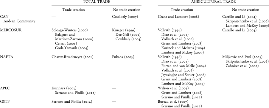
Our first hypothesis is that the profound regionalisation of farm trade in this period, which occurred in an international context of acute multilateral protectionism, and the relative failure of Latin American attempts to liberalise trade in the region could be a relevant part of the explanation of events. Farm and food products were fiercely protected by the industrialised nations in the post-war years, a situation that continued largely unchanged throughout the second half of the twentieth century.Footnote 4 Key to this was the exclusion of farm products from the successive negotiating rounds of the General Agreement on Tariffs and Trade (GATT).
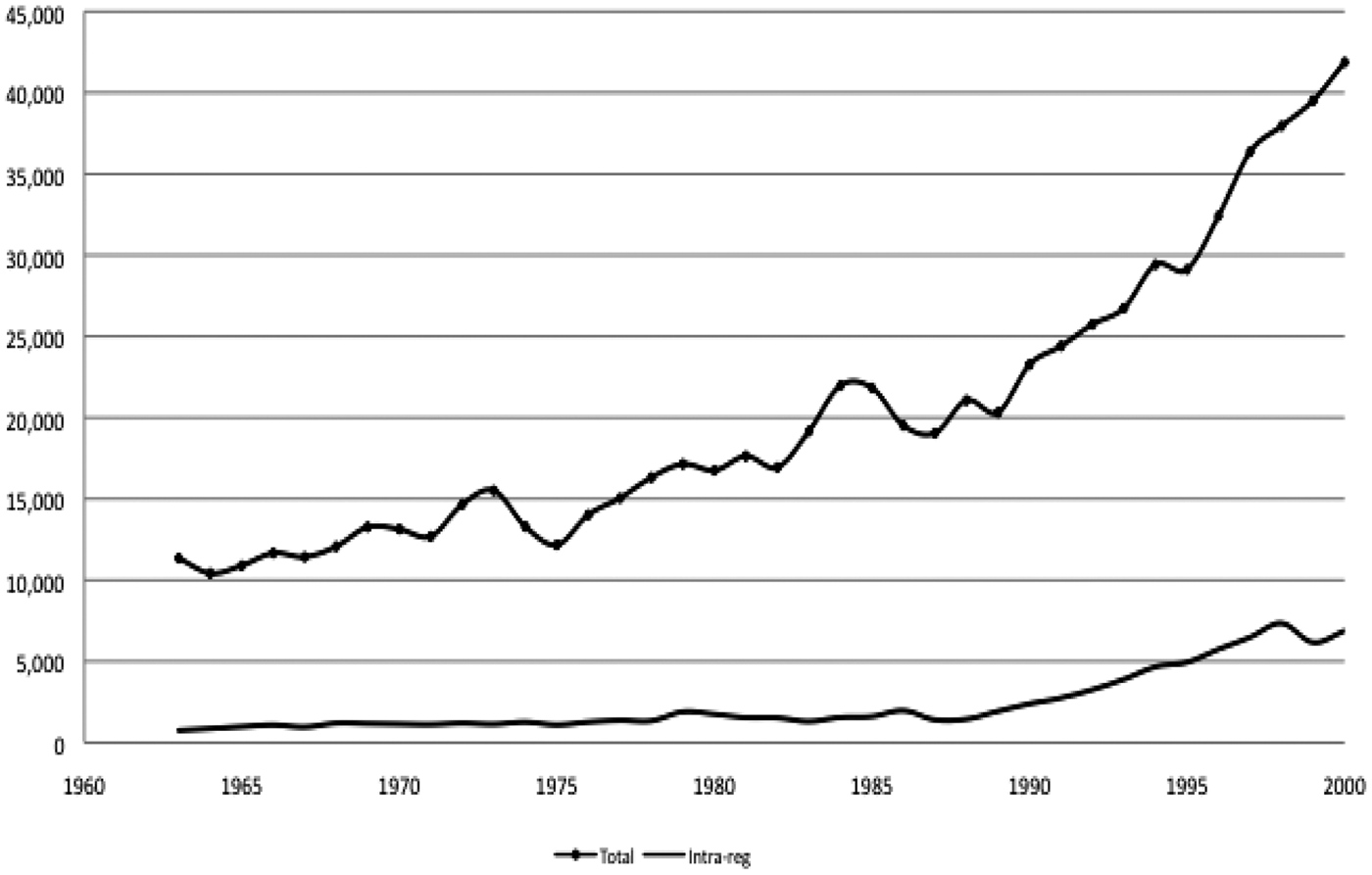
In this context, a significant part of the growth in farm trade occurred within regional blocs, and especially in the European Union. If the regionalisation of farm trade drove growth in Europe, it will be of interest to discover what results were produced by Latin American attempts at integration, even though the main goal of these moves was to strengthen the common market in manufactured goods. Despite the supposedly enormous potential of inter-regional farm trade, it in fact made up only 9 per cent of the Latin American countries' total volume of trade in agricultural products.Footnote 5 The trade stagnated at similar levels in absolute terms until the 1990s, resulting in an ongoing decline in percentage terms (see Figure 1 above).
Evolution of Latin American Agricultural Exports (Six Sample Countries and in Millions of 1985 US dollars)

The effects of the regional trade agreements have been widely discussed in the literature. However, there is little consensus on what these actually were. This study addresses the case of Latin American farm trade in particular, as once again there is no consensus view of the regional trade agreements' impact on this area.Footnote 6
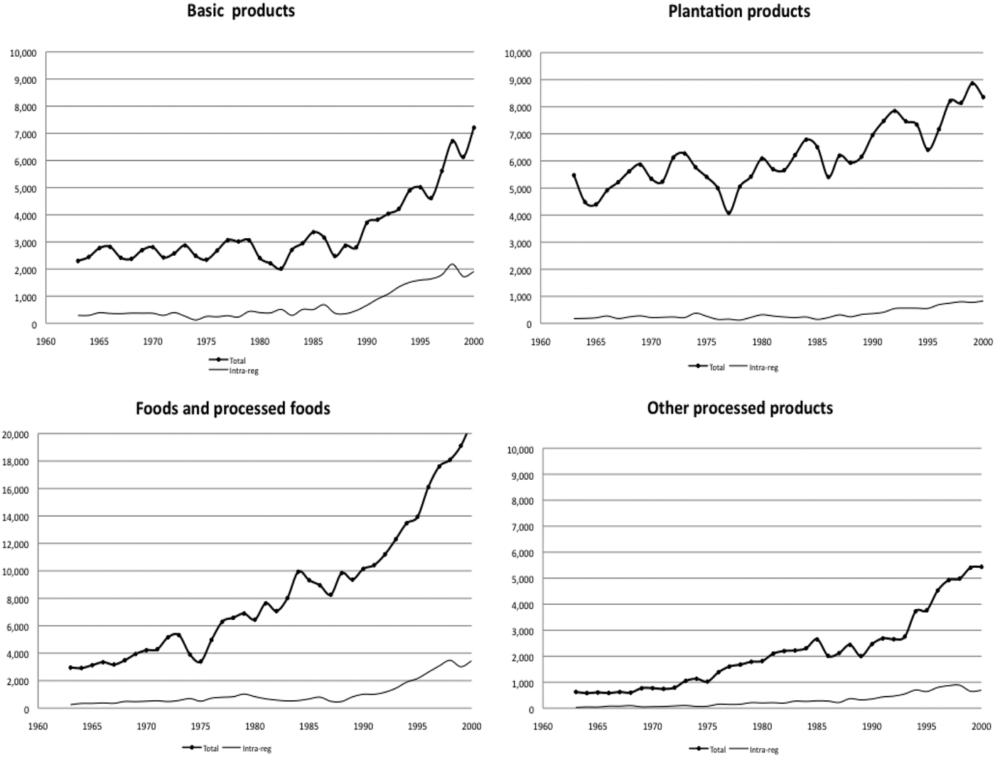
Second, we believe that Latin America's poor export performance might be explained by the focus of world trade on high value-added manufactured goods in the second half of the twentieth century (see Figure 2). As a result, the old inter-industrial trade model was supplanted by trade patterns that were predominantly intra-industrial. Together with a deterioration in relative prices, this explains the slow growth in farm trade as compared to overall world trade, as a result of which its percentage share shrank from 43 per cent of the total in 1951 to just 7 per cent by the end of the century.Footnote 7 Income growth in the developed countries brought rising demand for high income-elastic goods, to the detriment of spending on farm and food products, among which the best performers from a trade standpoint were precisely high value-added processed foods, which of course command the highest income elasticity. Latin American countries failed to make any major changes in the composition of their farm and food exports until very late in the day, and as a result they remained anchored to low-demand products. It was in fact only in the mid-1980s that any serious moves appeared that might allow them to escape this situation.Footnote 8 The contrasting example of Europe is revealing. Though they started from a position in which the relative share of high value-added products was fairly significant, the European nations tended to intensify specialisation.Footnote 9 In contrast, the countries of Latin America concentrated on commodities exports that had little chance of making headway in intra-industrial trade.
Evolution of Latin American Agricultural Exports by Product Group (Six Sample Countries in Millions of 1985 US dollars)
Our third hypothesis, which complements the two explained above, concerns the possible existence of a home market effect. Our study seeks to establish the home market effect involved in disaggregated Latin American farm trade flows. Footnote 10 In theory, a broad base of demand in the local market has positive effects on trade.Footnote 11 Growth in the domestic market and increasingly sophisticated demand patterns have the effect of increasing the range of production, so that countries with more dynamic home markets can also become net exporters of differentiated products. A key aspect of the model is that liberalisation and growth increase the localisation of firms in larger markets. The most efficient expand their output and export a differentiated product, leveraging economies of scale. This phenomenon is called the home market effect, and it is manifested where exports respond more sensitively to changes in the income of the exporting country than to the income of the importer. It has been shown that world farm trade grew fastest between 1963 and 2010 in the case of products which benefited from a home market effect.Footnote 12 The tardy shift in Latin American exports towards the kind of products that might enjoy such economies of scale would thus have hampered export growth.
To establish the scope of this hypothesis, we rebuilt the export flows of six Latin American republics to 39 countries (including the six exporters) in constant 1985 dollars between 1963 and 2000.Footnote 13 To sound a note of caution, our model is skewed towards the larger Latin American economies, which began with ISI policies earlier and stuck with them longer, and it includes all of the countries which Bulmer-Thomas refers to as the LA6 (Argentina, Brazil, Chile, Colombia, Mexico and Uruguay). This implies a bias towards relatively developed economies (for Latin America) with large domestic markets. However, it also means that the group under consideration accounts for more than two-thirds of total Latin American farm trade. To ensure that changes in domestic policies and in the international context are taken into account, we modelled the sub-periods 1963–1984 and 1985–2000 as well as the full period for the study.
We believe that this article will contribute to the existing literature by providing a study that covers a much longer time horizon than is usual and addresses more general issues, examining hypotheses which have not so far been tested for the second half of the twentieth century in Latin America. The study also makes some advances in the use of techniques for the calculation of gravity equations, using balanced panel data to avoid the bias found in cross-sectional studies and employing multilateral resistance terms to control for the effects of national trade policies.Footnote 14
Our findings suggest that the slow growth in Latin American exports of farm and food products compared with the growth in world trade was not a consequence of development policy alone but is also explained by other significant factors, namely the relative failure of attempts at economic integration in comparison with other regions, the low income elasticity of most exports and relatively stagnant domestic markets.
Latin America's Declining Role in World Farm and Food Trade
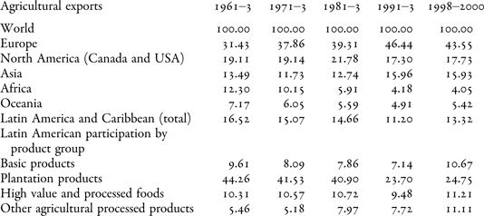
Latin America's relative share in world exports of food and farm products shrank inexorably in the second half of the twentieth century, and by the mid-1990s it was roughly half its pre-war peak, though it picked up in the first five years of the twenty-first century and the region succeeded in consolidating these gains at the end of the decade.Footnote 15 Meanwhile, average annual growth in total Latin American and Caribbean agricultural and food exports was only 3.2 per cent compared to 3.7 per cent for the world as a whole.Footnote 16 As Table 1 shows, the result was a decline in the region's relative share in the global total from 16.5 per cent in 1961–63 to just 11.2 per cent at the beginning of the 1990s. This was followed by a small recovery.
Latin America in the International Trade of Agricultural and Food Products (Percentage of World Trade in 1985 US dollars)
Source: Authors' compilation from FAO, Trade Yearbook (Rome: FAO, 1947–2000) and FAOSTAT, FAOSTAT Agriculture Database (2004).
Europe includes trade from the USSR and after 1991 from Russia and the ex-Soviet economies. North America includes Bermuda, Canada, Greenland, Saint Pierre and Miquelon, the United States.
Based on Table 1, we may conclude that exports shrank across the board until the 1990s with the sole exception of ‘other processed farm products’, and this decline was particularly marked in ‘plantation commodities’ (sugar, coffee, cocoa and tea), despite their traditional role as the sheet-anchor of agricultural exports from the tropical parts of the region.Footnote 17 The flip-side to the contraction in exports from Latin America and other regions was the spectacular growth achieved by the economies of the rich world, especially Europe.
Meanwhile, Latin America's export weakness limited its capacity to finance basic imports needed for the process of industrialisation. Stronger performance might, then, have mitigated some of the problems caused by external imbalances in many of the region's countries.Footnote 18
The feebleness of these export dynamics can be explained partly by institutional developments and trends in economic policy, both internationally and in the Latin American nations themselves.
On one hand, an essential change occurred in agricultural policy, as the developed nations began to increase their support for farming in the 1950s, while the developing world tended to penalise the sector.Footnote 19 In Europe, the Common Agricultural Policy (CAP) created a tightly controlled and heavily protected internal market in the European Economic Community (EEC) in pursuit of self-sufficiency in food production, offering spectacular incentives to producers whose enormous surpluses were unceremoniously dumped on international markets, seriously distorting trade.Footnote 20
Meanwhile, export-led agriculture was penalised by ISI policies,Footnote 21 which were clearly biased against exports, giving pride of place to support for industry while sidelining overseas trade in agricultural and food products. The resulting impact on agricultural prices was largely a sub-product of this development strategy, hurting the region's most competitive producers, who received only meagre compensation in the form of official farm loans and fertiliser subsidies.Footnote 22
Policy focused on measures to protect national output, including high tariff barriers, the imposition of occasional export taxes, indirect taxation of agriculture as a by-product of industrial protection and overvaluation of the currency. These policies caused a major transfer of resources away from agriculture. The resulting net outflow between 1960 and 1984 has been estimated at 85 per cent of agricultural GDP in Argentina, 56 per cent in Chile and 42 per cent in Colombia.Footnote 23 The goals, of course, were to hold down food prices, assure the domestic food supply in the cities and foster the process of industrialisation.
In contrast to outcomes in the developed world, these bureaucratic structures resulted in negative rates of protection for agriculture, especially in the initial decades of the ISI period. Reasonably reliable estimates exist of the impact of these polices on agriculture in a significant group of Latin American nations between 1965 and 2004. The figures are telling: the nominal rate of assistance (NRA), defined as ‘the percentage by which government policies have raised gross returns to producers above what they would be without government intervention (or lowered them, if the NRA is below zero)’ was negative in weighted average terms in the Latin America countries examined (Argentina, Brazil, Chile, Colombia, the Dominican Republic, Ecuador, Mexico and Nicaragua) between 1965 and 1989. Hence public policy depressed farm incomes by between 7 and 21 per cent in this period. Support in the subsequent years was minimal, at no time exceeding 5 per cent of farm incomes. Even more striking is the tremendous anti-trade bias. Breaking farm output down into import-competing and exportable products, we may observe that the former enjoyed significant, positive protection throughout practically the whole of the period (1965 to 2004), despite wide variations in actual levels of support, while the latter were unremittingly disadvantaged, despite a fall in the penalty from around 25 per cent in the 1980s to less than 5 per cent by the 1990s. Finally, the relative rate of assistance (RRA), constructed as the ratio between the nominal rates (NRA) for farm and non-farm products, reveals a strong anti-farm bias in the policies followed in Latin America until the 1980s.Footnote 24 It was only the reality of economic crisis and mounting foreign debt during this decade that finally changed this development strategy.Footnote 25 The new strategy involved mobilising resources in competitive export sectors, including agriculture. However, this volte-face itself involved the application of numerous interventions in the farm sector, which again varied widely from country to country.Footnote 26
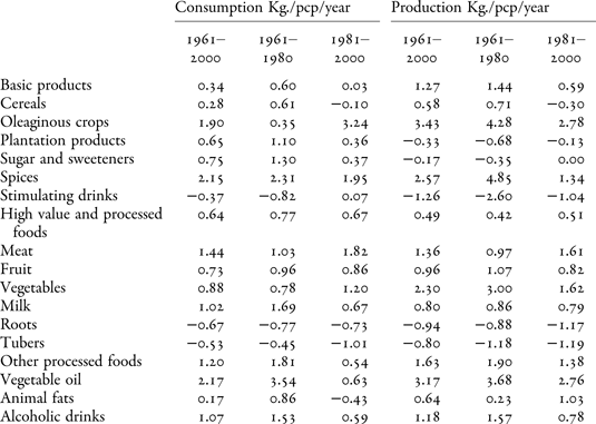
In this context, significant output growth was achieved, driven by the expansion of domestic demand, the technological gains provided by the ‘Green Revolution’, and the protection afforded to products destined for consumption in the home market.Footnote 27 From a long-term standpoint, per capita agricultural growth rates were around the world average and sometimes even higher in those countries where farmers enjoyed greater government support.Footnote 28 According to our calculations (Table 2), output growth was exceptional in the case of products for which demand was rising in Latin America (oil seeds, vegetable oils, alcoholic beverages, meat, vegetables and fruit, and dairy products), but very slow for the main agro-export crops (caffeinated beverages and sugar). It would seem reasonable, then, to argue that ISI policies resting on the competitiveness of Latin American agriculture and tariff barriers caused a shift in farm output, subordinating the sector to the needs of the industrialisation process. As a result, the region's imports of farm and food products grew more slowly than world imports until the end of the 1980s. In fact, its initially small share in the total shrank still further, as happened also in the case of exports.Footnote 29
Evolution of Per Capita Production and Per Capita Consumption of Agricultural and Food Products in Latin America (Annual Average Rates of Growth)
Source: Authors' elaboration on the basis of FAOSTAT, Agriculture Database.
The intense growth in international trade in the second half of the twentieth century can be explained in large part by the sharp cuts in protectionist tariffs achieved by the successive rounds of the GATT. However, agriculture was permanently protected from 1947 onwards, having been expressly excluded from the negotiations. It was in fact only in the early 1990s that a timid process of liberalisation began with the Uruguay Round.
In this protectionist context, the rapid spread of regional trade agreements had an expansive effect on aggregate international farm trade, sparking an intense process of regionalisation. In particular, the newly created European Economic Community (now the European Union) proved particularly successful in securing trade liberalisation and growth among its members. In the food and farm sector, intra-EEC trade between the member states accounted for just 17 per cent of total world agricultural trade when the community was founded. By the end of the twentieth century, the figure was close to 30 per cent.Footnote 30
Meanwhile, numerous integration processes were undertaken to bring regional markets together in Latin America. The first such endeavour was the formation of the Asociación Latinoamericana de Libre Comercio (Latin American Free Trade Association, ALALC or LAFTA) by the Treaty of Montevideo in 1960, which combined the economies of South America and Mexico. Around the same time, the countries of Central America, except for Panama, established a Mercado Común Centroamericano (Central American Common Market, MCCA) in the early 1970s. The Comunidad del Caribe (Caribbean Community, CARICOM) was formed in 1973. These early regionalist initiatives gradually foundered, however, and the failure of LAFTA led five of its members to form the Andean Pact in 1969, seeking to establish a customs union and create a free trade area. This organisation was subsequently redefined in 1980 as the Asociación Latino Americana de Integración (Latin American Integration Association, ALADI), which was intended to foster gradual integration, although it too failed to achieve significant trade liberalisation.Footnote 31 Such schemes at last began to enjoy a measure of success in the 1990s, which saw a revival of regional initiatives and a shift towards more open positions. The various sub-regional agreements made in this period held the key, chief among them the North American Free Trade Agreement (NAFTA) of 1994 and the Mercado Común del Sur (Southern Common Market, MERCOSUR) of 1991, which was a continuation of the failed ALALC and ALADI initiatives. At the same time, reforms were made to various existing arrangements like the Andean Pact, which became the Comunidad Andina in 1997, the Caribbean Community (CARICOM) and the Mercado Común Centroamericano (MCCA). Two of the region's countries, Mexico and Chile, also embarked upon a major push for integration, signing numerous bilateral free trade agreements, Mexico in 1995 with Costa Rica, Bolivia, and Venezuela and Colombia (G3), and Chile more gradually with Mexico, Colombia, Ecuador, MERCOSUR and Peru. There was also a strong supra-regional drive, which saw Mexico join the Asia-Pacific Economic Cooperation Forum (APEC) in 1993, followed by Chile in 1994 and Peru in 1998, and the accession of Argentina, Brazil, Colombia, Ecuador and Nicaragua to the Global System of Trade Preferences (GSTP) among developing nations in 1989. This brief review of integration efforts would be incomplete without a mention of two initiatives that would have no impact in the period with which we are concerned, but which are nonetheless important. These are the agreements made by Chile, Mexico and the members of MERCOSUR with the European Union, and the treaties establishing the Área Libre de Comercio de las Américas (Free Trade Area of the Americas, ALCA or FTAA).
A further key factor was the growth of trade in high value-added processed agricultural and food products at the expense of the tropical commodities which had historically formed the basis for trade. Per capita income growth meant that income-elastic processed products became increasingly important in diets all around the world.Footnote 32 Furthermore, products of this kind are mostly traded between rich nations, and in the latter decades of the twentieth century these flows outgrew general agricultural trade, benefiting from a certain intra-industrial effect.
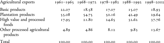
However, the products that predominated in the Latin American export mix were precisely the worst performing commodities in international markets. Table 3 shows the percentage share of each agricultural product group in Latin American exports. As may be observed, ‘basic products’ and ‘plantation products’ made up around 70 per cent of the total throughout most of the period, and they still account for a significant portion even at the end of the twentieth century, despite the decline in their relative share.
Composition of Latin American Agricultural Exports (Percentage of Trade in 1985 US$)
Source: Authors' compilation on the basis of FAO Trade Yearbook and FAOSTAT Agriculture Database.
Finally, rapid population growth eroded Latin America's traditional position as a net exporter of farm products.Footnote 33 The region has seen spectacular growth in demand for food and farm products, which is explained by the increase in the number of its people, growth in urban and industrial demand, and changes in consumption patterns. As a consequence, agricultural output destined for the domestic market outgrew export crops at least until the 1970s.Footnote 34
The population of Latin America increased faster than the world average at least in the early decades of the period, and it easily outstripped earlier periods of growth. Moreover, per capita food intake also rose sharply, putting considerable pressure on the farm sector to keep up the food supply, a phenomenon that weakened the region's traditional export capacity in the long run. In some cases, explicit export restrictions were applied to ensure that domestic demand could be met.
According to FAOSTAT data, average food consumption in the region in 1961–63 was only just above estimated nutritional needs at around 2,300 calories per capita per year, well below the 2,800 calories observed in the developed world, with which Latin America would gradually converge in the ensuing decades. Economic development in the form of industrialisation and urbanisation brought with it a clearly visible shift in food consumption patterns in Latin America. As may be observed in Table 2, the substantial improvement in calorie intake was determined on the one hand by the still rising consumption of vegetable foodstuffs (cereals, oil seeds and vegetable oils), and on the other by the sharp increase in the consumption of meat and dairy products.
Theoretical Model
We will use a gravity model to verify the hypotheses proposed. This methodology has been widely employed to investigate the principal determinants of trade. Its main advantages are its explanatory power with regard to bilateral trade flows and the stability of the results obtained. The functional specification of the model utilised here largely follows the work of Anderson, Bergstrand and Anderson, and van Wincoop, and it takes account of the phenomenon of ‘multilateral resistance’.Footnote 35 Applying logarithms, the functional formula is:
 $$\eqalign{ ln{\rm} X_{ij} &= {\rm} \beta _1 + {\rm} \beta _2 ln\left( {Y_i} \right){\rm} + {\rm} \beta _3 ln\left( {Y_j} \right){\rm} + {\rm} \beta _4 ln\left( {Va{\rm} \,pw_i} \right){\rm} + {\rm} \beta _5 ln\left( {Ypcp_j} \right){\rm} \cr & \quad+ {\rm} \beta _6 lnDist_{ij} + {\rm} \beta _7 lnExcvol_{ij} + {\rm} \beta _9 Border_{ij} + {\rm} \beta _{10} Lang_{ij} + {\rm} \beta _{11} RTA_{ij} \cr & \quad+ \beta _{12} D{\rm} \_UE_{ij} + \beta _{12} GATT_{ij} + \delta ^{} _i + \delta^{} _j + \varepsilon _t} $$
The base of the gravity equation is represented in the first place by Xij, which denotes the volume of the trade flow between a pair of countries. Yi Yj represents the size of the country markets, which is usually approximated in terms of GDP. Separate interpretation of this variable allows observation of each country's capacity to offer (export) products depending on its size measured by GDP, while potential foreign demand for the products will depend on the size of the importing country's market (GDP).Footnote 36
These variables can also be used to examine the effects of growth in the domestic market on trade flows. Such impacts will occur where exports are more sensitive to changes in the GDP of the exporting than of the importing country, a phenomenon known as the home market effect, which occurs in a scenario of increasing returns to scale and product differentiation. When countries trade, the partner with the largest market will produce a greater variety of goods, because it will attract more firms and will become a net exporter of differentiated products.Footnote 37
In contrast, the effect of slower domestic GDP growth in the exporting rather than the importing country (or null or negative growth) would fall within the scope of models describing trade in commodities and other undifferentiated products, the theoretical basis of which is more easily reconciled with models of reciprocal dumping.Footnote 38 This represents a situation in which price discrimination between the domestic market and international markets produces back and forth trade flows in the same product, as firms are able to benefit from greater elasticities in the international than in the domestic market.
Per capita income in the importing country is also included as Ypcp j, which denotes the type of good traded. Normal goods take a positive sign and inferior goods are negative.Footnote 39 Meanwhile, per capita income in the exporting country can be substituted by agricultural value added per worker, Va pw i, to adapt the gravity equation to the specific case of agricultural trade. This variable should reflect the effect of agricultural productivity on farm exports. A positive sign is expected.
The majority of studies also use numerous other variables simultaneously, including geographical proximity (whether or not the countries examined share a common border) and cultural ties (existence of historical or cultural links between trading partners, such as a common language). These variables may be expected to take a positive sign, given their ability to drive trade. In contrast, Dist ij, is the geographical distance between countries, which is normally considered an obstacle to trade and is treated as approximating transport costs.
As in the majority of published papers, the institutional context is difficult to model, because relevant data are either too sketchy or non-existent. In line with recent research, however, we have included multilateral (price) resistance terms in the model, which are approximated for each country concerned by the fictitious variables δ i + δ j, following the alternative proposed by Feenstra to the contributions of Anderson and van Wincoop.Footnote 40 These variables reflect barriers to trade that are either omitted or ignored by other variables, and this approach at least means they can be considered. In this case, their inclusion allows us to control for the effects of national economic policies on relative prices. This is especially useful to observe the impact of ISI policies on bilateral trade flows in the first of the two sub-periods analysed.
Finally, dummy variables were included to examine the effects of regional trade liberalisation, which was driven by the proliferation of regional trade agreements (RTAs), and of the multilateral liberalisation of international markets. RTA ij is a dummy variable taking a value of 1 if both countries in each pair are members of the same regional trade agreement and 0 otherwise. This allows us to examine the effects of membership of free trade institutions in the six Latin American economies examined based on the year of their accession to CAN, MERCOSUR, NAFTA, G-3, APEC and GSTP. Footnote 41 A significant positive value for this variable would show that membership of the same RTA generated trade, but a negative value would reflect a brake on exports. We also include a dummy variable (D_EU) to throw light on the effects in Latin America of the trade distortions caused by European integration.Footnote 42 A negative, statistically significant value for this variable would indicate the substitution of trade flows from non-EC nations by trade between the European partners.
Gravity models also frequently include dummy variables exploring the effects of membership of free trade organisations in order to shed light on multilateral trade liberalisation processes.Footnote 43 In our case, the value and sign of this variable are uncertain.
Finally, certain papers also include measures of the volatility of bilateral exchange rates with the aim of examining the impact of exchange rate uncertainty on trade flows. This variable is expected to take a negative sign. Hence, trade growth between a country pair will be lower in the face of exchange rate instability.
Data and Calculation of the Model: Bilateral Trade Flows
Let us now calculate the gravity equation for the bilateral trade data. To this end, we rebuilt volume export flows between 1963 and 2000 for a representative sample of the farm trade carried out by the six Latin American countries studied based on four product groups, namely basic commodities, plantation commodities, high value and processed foods, and other processed farm products.
The sample includes export flows for total farm trade and for the four product groups mentioned above between Argentina, Brazil, Chile, Colombia, Mexico and Uruguay, and between these six Latin American countries and 34 other representative importing nations in different economic regions. The database used is a balanced panel containing 8,892 observations (38 years × 6 × 39). The levels of representativity were more than acceptable in the 38 years spanned by the study, at all times staying above 70 per cent in the case of regional agricultural trade and rising to more than 90 per cent in the latter decades. As Figure 1 shows, the six countries' exports follow the same basic pattern as total agricultural trade in the region. Growth was relatively slow until the mid-1980s, dipping after the two energy shocks and then rising sharply in the 1990s, when exports to regional trade partners and to Asia grew rapidly.
Let us now explain the data used here.Footnote 44X ij consists of bilateral export flows provided by the UN-COMTRADE (2003) database published by the United Nations Statistics Division.Footnote 45 We followed the Standard International Trade Classification (SITC rev. 1) using data on flows from country i to country j. These flows were deflated by the respective price indices in the countries concerned in order to obtain series by volume and in 1985 US dollars. Y iYj denotes the real GDP both of the exporting nation and of the importer in 1985 US dollars (WDI cd-rom, 2004). Va pw i and Ypcp j respectively denote agricultural value added per worker in the exporting country and per capita income in the importing country, in both cases expressed in 1985 US dollars (WDI cd-rom, 2004). Dist ij is the distance between the capital cities of the exporting and importing countries (CEPI-Database). Excvol ij is an indicator of exchange rate volatility constructed as the standard deviation of the first difference in the natural logarithm of the nominal bilateral exchange rate in the ten years preceding period t (WDI cd-rom, 2004). Border ij is a dummy variable which takes a value of 1 if the countries share a common border and 0 otherwise. Lang ij is a dummy variable which takes a value of 1 if the countries share a common language and 0 otherwise (CEPI-Data Base). GATT ij is a dummy variable which takes a value of 1 if both countries in a pair are members of the GATT and 0 otherwise. RTA ij is a dummy variable taking a value of 1 if both countries in a dyad are members of the same regional trade agreement and 0 otherwise.
Our aim is to overcome the limitations of previous studies, which in most cases only take into account variations between the units observed (cross-sectional analysis). Here, however, we will also consider changes arising over time within the units observed. In this regard, the use of panel data increases the efficiency of estimators and significantly reduces potential problems associated with the omission of variables.Footnote 46 Three procedures were applied to the panel data. The first consisted of calculating minimum least squares (MLS) with grouped panel data, while the second and third addressed temporal variations by respectively including random effects and fixed effects in the model.
In order to determine which of the three models calculates the gravity equation most efficiently, we first applied the Lagrange multiplier test for Breusch-Pagan random effects to allow discrimination between the MLS calculation for the grouped panel data and calculation using random effects.Footnote 47 Having applied this procedure, we concluded that the random effects are relevant, and therefore that the random effects calculation is preferable to the grouped panel data procedure. We also performed a battery of tests to establish that the inclusion of fixed effects is more appropriate than the procedures described above. In the first place, the F-test of the significance of fixed effects suggests that these estimates are better than the results obtained from MLS calculation of the grouped panel.Footnote 48 Second, the Hausman test demonstrated that the estimators of random and fixed effects differ substantially, and that the fixed-effects model provides a better explanation of the sources of variations, making it more appropriate than the random effects model.
Despite our efforts to model temporal and spatial heterogeneity, our model still presents problems of heteroscedasticity according to the Wald test, and according to Woodridge's test there is also some autocorrelation. Finally, the Breusch-Pagan test used to identify possible problems of contemporaneous correlation in the residuals of fixed-effects models confirms the need to correct this problem. The above issues were resolved by calculating the model with panel corrected standard errors (PCSE).
At first glance, the models function well both for total agricultural trade and for the different bilateral trade groups considered. All of them are able to explain a significant percentage of the variations arising in agricultural trade flows. Furthermore, all of the variables take the expected signs, and in general trade flows are greater between countries with large, growing markets that are geographically close to each other, as the gravity equation predicts. Let us begin with a discussion of the results obtained for the distance variable (Dist ij), given that the calculation methods described below (PCSE calculation) require the elimination of variables that do not change over time. The variable is negative for products of all kinds, indicating the existence of significant obstacles to trade between distant markets.
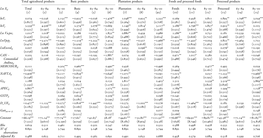
The first column of Table 4 shows the results obtained from the PCSE calculation, which analyses the factors determining the trend in Latin American agricultural and food exports.Footnote 49 As the model is expressed in logarithms, the coefficients shown for continuous variables should be interpreted as elasticities. To put this another way, the scores indicate the percentage increase in exports for each 1 per cent increment in the independent variables. The values obtained for the market size variable (Yi Yj) are highest on the side of the importing country, demonstrating its significance for exports. Meanwhile, the destination country (3.559, the score obtained for Yj) has a positive, statistically significant influence, representing the highest impact of all the continuous variables. This finding is related to growth in the demand for agricultural and food imports, which is known to be very high, especially in less developed regions, due to the sharp rise in calorie intake and the demographic boom. The results of the analysis by product groups reveal higher international demand for basic commodities (2.374), which include the staples of international diets, and in particular for high value and processed foods (3.286), which are mainly responsible for the shifts occurring in food consumption patterns over the period.
Results of the Gravity Equation
Note: Prais-Winsten estimations with PCSE and fixed effects The total is the aggregate of agricultural trade; basic: basic products; plantac: plantation products; foods: high value and processed foods; processed: processed products. All the variables are in logarithms, except for binary variables (regional trade agreements). The standard errors are in parentheses. ***, ** and * denote 1, 5 and 10 per cent of the level of statistical significance, respectively.
Perhaps the most interesting result is the non-statistically significant score of 0.074 obtained for the GDP of the source country (Yi) in the case of total agricultural exports, which validates one of our initial hypotheses, namely that growth in the size of domestic markets in the region had little effect on Latin America's farm export capacity. As explained in the second section, domestic demand for food expanded rapidly in the second half of the twentieth century, driven by population growth and improvements in diet. In the disaggregated analysis, we may observe that this effect was negative and statistically significant in the group of ‘basic products’, which includes cereals (−0.935), but positive and significant in ‘plantation products’ (1.048) and ‘other processed products’ (0.895).
Despite the positive sign observed in the latter two groups, however, Latin American agricultural trade did not benefit from any home market effect in the long run, and in no case are domestic market coefficients higher than export market coefficients. The contrast with the developed nations of Europe is striking: the expansion of these countries' markets had a major impact, proving even more important as a driver of exports than growth in their export markets as intense trade specialisation in industrially processed agricultural and food products created economies of scale and generated a home market effect.Footnote 50 Hence, the concentration of a vigorous agro-food industry in Europe, product variety and product differentiation combined to allow very rapid growth in farm exports. Our results, however, support the findings published in other studies of more recent periods, which describe a pattern in Latin America consisting of trade in very similar products.Footnote 51
Empirical analysis also reveals the negative impact of rising per capita incomes in the importing countries (value of Ycpc j) on Latin American export flows. This result demonstrates overall that the region's agro-export specialisation fundamentally consisted of basic goods. As may be observed, all of the product groups except for ‘other processed products’ display negative income elasticity of demand, and the scores are relatively high (−1.319 for ‘basic products’, −0.904 for ‘plantation products’ and −1.512 for ‘high value and processed foods’). Hence, rising income per head resulted in more than proportional falls in demand. Once again, the region performed worse than Europe and total world exports. The type of specialisation existing around 1960 appears crucial. While basic and plantation commodities accounted for 77 per cent of Latin American farm exports at that time, they made up just 40 per cent of Europe's.Footnote 52
Meanwhile, rising agricultural labour productivity (Va pw i) had a general, positive and statistically significant effect (1.012). This result may be related to technical progress in Latin American agriculture, and such productivity growth would have driven exports more or less proportionally.Footnote 53 Furthermore, the effect was greatest in the ‘high value and processed foods’ group of products (1.286) and then in ‘plantation products’ (0.880).
The variable included to analyse the influence of exchange rate volatility (Excvolij) in general presents very low scores which are not statistically significant.
The results obtained for the discrete variables, which only take values of 1 or 0, allow the calculation of semi-elasticities or to put this another way, they show the percentage increment obtained by switching trade partner from a country that is not a member of the same RTA to a member of such an agreement.Footnote 54 In institutional terms, these results confirm the patchy success of liberalising trade deals in Latin America in the long run. The values taken by the fictitious variables included in the model to measure the trade creation effects of Latin American integration processes (CAN, MERCOSUR, NAFTA, G-3, APEC and GSTP) show that these initiatives in general failed to generate trade, at least from the standpoint of aggregate farm exports. In fact, APEC is the only one to display any positive, statistically significant effect, while NAFTA threw up a significant negative value (−0.906), showing that the process of North American integration distorted the trade of the non-member Latin American nations. Thus, NAFTA depressed trade flows from non-member Latin American exporters to its member states by some 60 per cent.
Turning to a more detailed analysis of farm product groups at the disaggregated level, we may observe positive, statistically significant effects from trade liberalisation in APEC (also observable at the aggregate level, as mentioned above), particularly in ‘basic products’ and ‘foods and processed foods’. Such effects are also visible in CAN for ‘foods and processed foods’, in G3 for ‘plantation products’ and ‘other processed products’, and in MERCOSUR and GSTP for ‘basic products’. Contrary to the findings described by Soloaga and Winters, our results reflect trade distortion in the case of NAFTA, not only in aggregate but also for all of the product groups analysed, in line with the conclusions of Grant and Lambert.Footnote 55
The dummy variable D_UEij also reveals a trade distortion affecting Latin American exports, reflecting the impact of European integration. The values displayed by aggregate trade (−0.477) and in particular trade in ‘basic products’ (−0.816) are negative and statistically significant, indicating an appreciable downside effect for the countries of Latin America, causing their aggregate exports of agricultural products to the EC member states to shrink by some 38 per cent and exports of basic commodities to plunge by 56 per cent. This illustrates just how important the European customs union was for third parties, because the process not only removed trade barriers between the EC partners, allowing an expansion of trade, but it also raised the tariff wall against outside imports. The results obtained for the Gatt 94-00 variable reflect the nugatory impact of GATT membership on the aggregate agricultural exports of Latin American countries and their trade partners, even after the Uruguay Round. The agreements reached at the Uruguay Round in fact had positive effects only from a disaggregated standpoint for ‘plantation products’ (0.391, representing a 48 per cent increase in exports) and for ‘other processed products’ (0.491, generating a 63 per cent rise in exports). These two results reflect the high levels of protection facing Latin American exporters throughout practically the whole of the period, which made it difficult for them to perform better in their target markets. The exclusion of agricultural products from the GATT agreements almost until the end of the century had a high cost for countries specialising in farm exports.
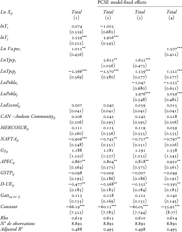
The model is reasonably robust. The sensitivity analysis performed on the results, shown in Appendix Table 2,Footnote 56 demonstrates that the results of different combinations of variables (GDP and per capita income; per capita income and population) do not reflect significant changes for the RTAs considered. The fictitious variables reflect similar values, the same sign and the same statistical significance as explained above.
In order to take our analysis further, we split the study period into two sub-periods (1963–83 and 1984–2000), calculating the gravity equation for the exports of the six Latin American countries using a similar methodology and variables.Footnote 57 These two sub-periods were very different. To begin with, ISI policies were in full swing in the first sub-period, which was followed by more open trade in the second. Second, the make-up of the region's agricultural exports also changed from the first sub-period to the second, as explained in the second section of this article.
Applying the same approach to calculation of the gravity equation, the tests performed once again pointed to PCSE as the best tool for this purpose.
The results obtained clearly show that the relative decline in Latin America's share of world farm trade was caused by events in the first sub-period. There were three main reasons for this: the export mix was strongly skewed towards the least dynamic products; domestic markets did little to drive exports; and early Latin American trade agreements enjoyed scant success.
In the first place, the export mix had a negative influence on growth, as shown by the negative sign and high value of the per capita income variable for the importing country. Thus, demand for Latin American specialities tended to fall as incomes rose in the importing nations.
Meanwhile, growth in the domestic market had no impact on exports (consider the negative values for Yi both in aggregate farm trade and basic commodities).
Finally, the variables designed to capture the effects of regional trade initiatives are statistically significant only in the case of CAN (which displays a low but positive and significant score for ‘plantation products’), confirming that attempts at integration between the 1960s and the 1980s had almost no effect.
In the second sub-period, and particularly after the end of the turbulent 1980s, Latin America regained lost ground in international farm trade. This was possible thanks to a change in the mix of exports, resulting in significant gains in the share of high-value products and a decline in the share of basic and, especially, plantation commodities. While the per capita income variable remains negative for importing countries, the score is much lower and is no longer significant, indicating that per capita income growth in importing countries no longer depressed demand for Latin American agricultural exports as a whole.
Furthermore, the model displays a positive effect from the domestic market variable Yi, which displays a positive and significant score for total agricultural trade (2.152), ‘plantation products’ (2.352) and ‘other processed products’ (3.059). Even more important is the home market effect reflected by higher scores for the exporter's GDP than for the importer's, both for aggregate farm trade and for ‘processed products’. The shift in development strategy that began in the 1980s was accompanied by significant changes in the composition of agricultural trade resulting from the move towards a strategy of reintegration in international markets. In a more integrated economy that is more open to competition, consumers enjoy access to a wider range of goods and each company (country) exports differentiated products, generating benefits from economies of scale. Trade liberalisation processes are known to be related to the relocation of firms towards larger markets, where they can exploit economies of scale and export differentiated products.
Finally, regional integration initiatives finally began to bear fruit. Thus, the liberalising drives of the 1990s are echoed in the positive trade creation effects observable in MERCOSUR (aggregate, basic commodities and food), the G3 (plantation commodities, food and processed food), APEC (basic commodities and other processed products) and GSTP (basic commodities). In addition to this result, the trade distortions produced by the EC were less severe than in the first sub-period, and the result was that the agricultural exports of the Latin American six met with less protected markets and lower penalties in a key destination. Meanwhile, the European Union took the decision to relax agricultural protection, resulting in a certain decline in agricultural output.Footnote 58
Conclusions
This article analyses the factors determining the evolution of Latin American agricultural exports and the impact of the development strategies followed in the second half of the twentieth century. To this end, we applied a gravity equation to agricultural trade flows. Our analysis is unique, insofar as very few published papers have focused specifically on the trade in farm products, and those that have done so generally lack a long-term perspective like that presented here. Furthermore, none of them disaggregates trade by product groups.
Returning to our early hypotheses, we have confirmed from a long-run perspective that regional trade liberalisation initiatives had little effect in driving agricultural trade in an environment of highly protected markets. Regional trade organisations not only failed to create an integrated market in the new industrial goods produced as a result of the import substitution strategy applied in the early decades of the period, but they also proved unequal to the task of achieving any significant integration of markets in agricultural and food products. It was not until the mid-1980s, in fact, that intra-regional agricultural trade took off, and in the interim exports of agricultural products faced highly protected markets within Latin America itself. A wider, integrated regional market might have encouraged specialisation and an early move towards higher value-added and differentiated agro-industrial products, providing an incentive for productivity gains, as occurred in Europe.
However, we have found that the resurgence of integration initiatives in the 1990s was more successful, especially in the cases of MERCOSUR and G3. Intra-regional trade in farm products grew rapidly at this time. The biggest success stories, however, were agreements like APEC and GSTP between very different economic structures, which provided the opportunity to supply wider markets, driving technological progress and agro-industrial development.
In the second place, the export mix had negative effects on growth. From a long-term standpoint, specialisation occurred in goods with negative income elasticities of demand.
Finally, we have been able to show that there was no home market effect over the period as a whole, so that the region largely failed to find a role in the new dynamic patterns of intra-industrial international trade that arose during the period.
The disaggregated analysis for the two sub-periods considered here revealed the importance of the change in the mix of Latin American agricultural exports, which began in the mid-1980s, and of the improved performance of the region's domestic markets.
These phenomena had a positive influence on exports, driving the transformation of agro-industry, due to the greater size of the internal market and the switch to products which had less negative income elasticities overall than traditional commodities exports. In some product groups, indeed, the income elasticity of demand was even found to be positive.
It seems clear, then, that the shift in development strategy that began in the 1980s was accompanied by significant changes in the composition of farm trade resulting from the move towards a strategy of reintegration in international markets.
We were also able to confirm that the growth of agricultural exports was driven mainly by the expansion of foreign demand attributable to income growth in importing nations, and by technological development, which raised the productivity of farm labour. In contrast, geographical distance and protectionism in key export markets hampered growth. Moreover, the rise of regionalism and integration processes in North America and Europe distorted trade by encouraging exchanges between member states to the detriment of non-member nations, an effect which was not offset by multilateral liberalisation of agricultural trade via the GATT. The high levels of agricultural protectionism practised by the developed nations indubitably spurred inward-looking economic strategies based on industrial development. The progressive abandonment of these policies therefore required greater liberalisation of developed-world markets. In turn, the surge in farm exports towards the end of the 1980s reinforced the change of strategy, placing agro-industry once again at the heart of many Latin American economies.
Although strongly representative of Latin America as a whole, the sample of countries selected for this study is clearly biased towards the larger, more developed economies, which were the most determined to pursue the ISI route. Hence, the underrepresentation of small, less developed nations is one of the limitations of this study.
The incipient changes in Latin American agricultural and food trade in the last decade of the twentieth century have gathered pace since then. Specialisation has intensified, and regional integration efforts have continued to bear fruit. In turn, buoyant Asian demand for commodities and foodstuffs has introduced a new factor, affecting basic products in particular. In this light, we intend to continue this research by looking specifically at these changes and their consequences for the economies of Latin America. Also, the present study does not consider the behaviour of export prices and their effects on trade and development opportunities, a central issue in debates about the economy of Latin America. We plan to address this question as our next objective, building a specific price series for agricultural exports in order to contribute to the debate about the implications of the terms of trade for the region's development.
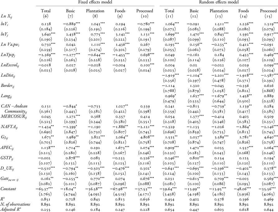
Gravity Equation Results: Latin American Trade Disaggregated by Product Groups (Fixed Effects and Random Models Not Presented in Table 4)
Results of the Gravity Equation: Sensitivity Analysis Including Population
Regional Trade Agreements Analysed in the Econometric Model
The Controversial Debate on the Effects of Integration Processes in Latin America