





1. Introduction
1.1. Motivation
The generation and propagation of acoustic waves and instabilities in compressible flows, and in shear flows in particular, have a long history of research. Understanding the role of unstable growing and neutral non-growing acoustic waves in noise generation in free shear flows can provide a basis for improving flow behaviour in various engineering applications, especially in the aerospace sector, since the basic properties of compressible shear-layer flow reappear in jet flows and mixing layers, among others. In the current work, we focus on instabilities.
1.2. The Pridmore-Brown equation and stability analysis
Due to the essentially inviscid character of acoustic waves, the linearised Euler equations (LEE) are commonly employed to identify the basic properties of acoustic waves. The seminal work on compressible stability theory was done by Lees & Lin (Reference Lees and Lin1946), who provided a general stability criterion depending on the gradient of the product of density and vorticity, analogous to the Rayleigh–Tollmien criterion for an incompressible fluid. In order to analyse and mimic the occurrence and propagation of small (acoustic) perturbations in plane parallel shear flows, Pridmore-Brown (Reference Pridmore-Brown1958) formulated a normal-mode approach as a solution of the LEE. From that, a second-order ordinary differential equation (ODE) results, which was later named the Pridmore-Brown equation (PBE). The PBE has since then been used to study instabilities and wave propagation. Besides the numerical treatment of inviscid equations by means of contour deformation and shooting methods (Mack Reference Mack1990), analytical solutions turned out to be useful. Since the first analytic asymptotic solutions of the PBE were given in the original work of Pridmore-Brown (Reference Pridmore-Brown1958), various authors formulated analytic solutions for various velocity profiles. The first solution was probably found for a plane vortex sheet by Miles (Reference Miles1958), and since then exact solutions have been formulated in terms of special functions or Frobenius series, for example by Goldstein & Rice (Reference Goldstein and Rice1973), Jones (Reference Jones1977) and Campos (Reference Campos1999) for a linear shear flow, Campos & Kobayashi (Reference Campos and Kobayashi2000) for a hyperbolic tangent shear layer and Zhang & Oberlack (Reference Zhang and Oberlack2021) for an exponential boundary layer. Special functions as solutions of ODEs are usually characterised by the number of singularities of the ODE (Olver et al. Reference Olver, Lozier, Boisvert and Clark2010).
In order to have a realistic model of a free shear layer, the hyperbolic tangent velocity profile was first used by Michalke (Reference Michalke1965), who numerically studied spatially growing perturbations. The hyperbolic tangent is a good model for the mixing region in a coaxial jet engine exhaust (Maslowe & Perrault-Joncas Reference Maslowe and Perrault-Joncas2008). Regarding the linear stability of this flow, there exist a lot of works and we will highlight some of them. Blumen et al. (Reference Blumen, Drazin and Billings1975) were probably the first to find supersonic disturbances and to show that the hyperbolic tangent shear layer is unstable at any Mach number. Drazin & Reid (Reference Drazin and Reid1979) and Michalke (Reference Michalke1984) also investigated the stability behaviour of this flow and completed the picture of unstable supersonic disturbances. Extensive inviscid numerical calculations of unstable modes were done by a shooting method in the work of Mack (Reference Mack1990), which presently serves as a basis for the validation of our analytic results. As shown by Ragab & Wu (Reference Ragab and Wu1989) for the hyperbolic tangent mixing layer, viscous linear stability results tend to an inviscid limit for Reynolds numbers larger than
 $1000$
. A comprehensive classification of spatially unstable modes by means of their phase velocity was done by Jackson & Grosch (Reference Jackson and Grosch1989), who analysed the spatial stability of the hyperbolic tangent shear flow profile by means of a shooting method. They found above a critical Mach number two groups of instabilities, namely the so-called fast and slow modes, each of them supersonic with respect to one free stream. In addition to the papers mentioned above, many other researchers have recognised that compressible mixing layers in general, including the hyperbolic tangent profile, become less unstable when the Mach number is increased (Brown & Roshko Reference Brown and Roshko1974; Chinzei et al. Reference Chinzei, Masuya, Komuro, Murakami and Kudou1986; Lele Reference Lele1989; Sandham & Reynolds Reference Sandham and Reynolds1989). This is probably the most central result regarding the influence of the Mach number.
1.3. Stability and noise emission
Stability investigations are of great interest since flow instabilities give rise to unsteady phenomena causing noise and transition to turbulence and the previously mentioned work all contributed to that research field. However, a direct link between unstable modes, discussed in the previous section, and noise radiation was not established for a long time. This is because the boundary conditions chosen in stability analysis typically demand bounded perturbations in the far field where an observer would be located, i.e. far away from the shear zone. The shear layer acts as a waveguide for an instability mode, thereby trapping the mode and impeding sound radiation in the form of harmonic waves. However, considering more realistic models and extending the classical linear stability and parallel flow approximation, it is found that sound is emitted.
Pioneering work was done by Lighthill (Reference Lighthill1952), who investigated jet noise by developing the acoustic analogy. It is a rearrangement of the momentum and the continuity equations, where an inhomogeneous wave equation is obtained. The inhomogeneity contains linear and nonlinear sources and the effects of viscous and thermal dissipation. Thereby, a solution of Lighthill’s equation can be constructed using the principle of Green’s function. However, for this, the source terms have to be regarded as known, and their determination is the key issue. Especially with respect to the source terms, Lighthill’s acoustic analogy has since then been modified. Lilley (Reference Lilley1974) viewed all linear inhomogeneous terms in the inhomogeneity of the original formulation as representing sound propagation effects, i.e. convection and refraction of sound waves, and hence moved these terms to the left-hand side to formulate an improved analogy. Goldstein (Reference Goldstein2010) discusses this modification and derives it as a special case of a generalised acoustic analogy (Goldstein Reference Goldstein2003). Furthermore, Goldstein & Leib (Reference Goldstein and Leib2005) incorporate spatially growing linear instability waves in the Green’s function to ensure that the acoustic field is causal. The question which terms and effects have to be included in the source terms also depends on the Mach number and the high Mach-number regime is discussed by Goldstein & Mankbadi (Reference Goldstein and Mankbadi1993). According to their work, velocity fluctuations in the high Mach-number regime may decay as slowly as the acoustic waves themselves, which is why the coupling between these components must be considered in the formulation of the source terms. The source terms in the acoustic analogy can also be obtained by direct numerical simulations (DNS), as shown by Colonius et al. (Reference Colonius, Lele and Moin1997) for a compressible mixing layer, revealing the importance of flow–acoustic interaction. Increasing computational power, and thus new possibilities in DNS, also allow far-field radiation to be obtained directly from the solution if appropriate filters are used. However, the previous discussion makes clear that modelling the source terms in the acoustic analogy requires a prior knowledge of all interactions and effects. Even an approximation might be difficult to achieve (Wu Reference Wu2005).
The inherent weakness of acoustic analogies is that one must decide which terms represent sources and which terms represent sound propagation. This fact and the recognised importance of large coherent structures (Jordan & Colonius Reference Jordan and Colonius2013; Zhang & Wu Reference Zhang and Wu2020) in noise generation motivated various authors to reconsider the noise emitted by instability modes and turbulence. We will in the following highlight progress made using the method of matched asymptotic expansions. For a more extensive summary of the different fundamental approaches to jet and shear-layer noise, the interested reader is referred to the review by Tam (Reference Tam1995).
To achieve a connection between instabilities and noise generation, Tam & Burton (Reference Tam and Burton1984a , Reference Tam and Burtonb ) used the method of matched asymptotic expansions for both a two-dimensional shear layer and an axisymmetric jet. In their seminal work, they started with a neutral supersonic radiating mode, which emits a planar acoustic wave into the far field. Introducing spatial growth and decay of this mode, Tam & Burton calculated a Mach-wave beam from this mode, using the method of matched asymptotic expansions. The matching between the instability and the far-field propagating wave takes place at the edge of the shear layer or jet, near the far field. The results of this matching process show that instabilities with phase speeds that are supersonic with respect to the far field generate so-called Mach waves that radiate into the far field and the mechanism is called Mach-wave radiation. For the jet configuration, the results of Tam & Burton (Reference Tam and Burton1984b ) show good agreement with the experimental results of Troutt & Mclaughlin (Reference Troutt and Mclaughlin1982). Several extensions of the method of matched asymptotic expansions have since been made. Tam & Chen (Reference Tam and Chen1994) included a broad frequency spectrum by using a stochastic model to obtain the noise generated by large turbulent structures in jets. A further extension for shear flows with respect to nonlinearities was made by Wu (Reference Wu2005) and Wu & Zhang (Reference Wu and Zhang2019), who analysed how a nonlinearly modulated wave packet leads to acoustic waves in the far field, depending on the amplitude of this wave packet. Wu (Reference Wu2005) gave a full asymptotic characterisation of the Mach-wave beam and analytically related the acoustic far field with the nonlinearly developing amplitude of the mode. For this it is decisive that a supersonic mode nonlinearly interacts with the critical layer. For further insights into the theory of nonlinear interactions between shear flow instabilities and critical layers, the reader is referred to the review by Wu (Reference Wu2019). Apart from the supersonic radiating modes discussed previously, it should further be noted that a subsonic instability mode, trapped within the shear layer, also emits sound waves when considering its spatial amplification and decay (Zhang & Wu Reference Zhang and Wu2023).
To sum up, instabilities and coherent structures forming far-field radiating wave packets are crucial for noise radiation.
1.4. Aim and structure of the present work
The general link between acoustic wave propagation, reflection and instabilities motivated the current work. We further aim to complete the picture of unstable modes in the temporal case and thereby show how symmetry methods and in particular equivalence transformations are applicable to that eigenvalue problem. Symmetry methods provide a tool to save computing time and gain insights into how solution spaces for different physical situations are connected. By constructing Frobenius-series solutions for the PBE around its singularities and connecting them, we obtain the full picture of the linear mechanisms that lead to temporal instabilities. The method of connecting Frobenius series was in principle used before by Campos & Kobayashi (Reference Campos and Kobayashi2000) for the calculation of reflection and transmission coefficients in a shear layer. Connecting Frobenius power-series solutions at the critical layer to calculate eigenvalues was also the technique used by King et al. (Reference King, Brambley, Liupekevicius, Radia, Lafourcade and Shah2022). Our current work adds a transformation of the independent variable to map the infinite number of singularities to a finite one as well as an approach to solve eigenvalue problems. Through this new principle we exactly account for the singularities in the underlying differential equation. The singularities and their character are decisive for the occurrence of the modes and need to be fully considered.
This work is structured as follows: in § 2, we give an overview of the fundamental equations that describe acoustic fluctuations in a plane parallel shear flow and introduce the hyperbolic shear layer as a model which is analysed with respect to acoustic waves and instabilities. Section 3 is dedicated to the mathematical method used in this work. We discuss how an exact solution for the given flow field is constructed and present the connection algorithm based on Frobenius power series that allows us to treat eigenvalue problems. In order to extend the considerations to a more general class of three-dimensional (3-D) propagating modes as well as non-isothermal flows, we further present in § 4 how equivalence transformations allow us to use the method originally developed on the basis of the 2-D isothermal problem for a wider class of problems.
We finally discuss the results of the temporal stability consideration in § 5.
It should be noted that the theory of Briggs (Reference Briggs1964) probably provides the most complete understanding of instability, as it takes into account both temporal and spatial growth to determine the full response of the flow to a disturbance. Although the results in this work are given for temporal growth, the present method could be adapted to the more practically relevant case of spatial stability.
2. Fundamental equations
2.1. From Euler to Pridmore-Brown
In this section, we briefly review the derivation of the underlying equation, the PBE, introducing the relevant assumptions and governing equations. We focus on the basic linear phenomena contributing to noise emission. Since viscous effects may be neglected for fundamental acoustic phenomena (Rienstra & Hirschberg Reference Rienstra and Hirschberg2004), the PBE and the present analyses are based on the LEE, where primes denote small perturbations about a reference state, indicated by the subscript
 $0$
 \begin{align} \frac {{\rm D}_0 \rho ^{\prime }}{{\rm D} t}+\rho _0 \boldsymbol{\nabla } \boldsymbol{\cdot }\boldsymbol{v}^{\prime }+\boldsymbol{v}^{\prime } \boldsymbol{\cdot }\boldsymbol{\nabla }\rho _0+\rho ^{\prime } \boldsymbol{\nabla } \boldsymbol{\cdot }\boldsymbol{V}_0 =0,\end{align}
 \begin{align} \rho _0 \frac {{\rm D}_0 \boldsymbol{v}^{\prime }}{{\rm D} t}+\boldsymbol{\nabla }\!p^{\prime }+\rho _0 \boldsymbol{v}^{\prime } \boldsymbol{\cdot }\boldsymbol{\nabla }\boldsymbol{V}_0+\rho ^{\prime } \boldsymbol{V}_0 \boldsymbol{\cdot }\boldsymbol{\nabla } \boldsymbol{V}_0 =0,\end{align}
 \begin{align} \frac {1}{c_0^{2}}\left (\frac {{\rm D}_0 p^{\prime }}{{\rm D} t}+\boldsymbol{v}^{\prime } \boldsymbol{\cdot }\boldsymbol{\nabla }\!p_0\right )+\rho _0 \boldsymbol{\nabla } \boldsymbol{\cdot }\boldsymbol{v}^{\prime }+\left (\rho _0 \frac {c'^{2}}{c_0^{2}}+\rho ^{\prime }\right ) \boldsymbol{\nabla } \boldsymbol{\cdot }\boldsymbol{V}_0 =0.\end{align}
We assume a homogeneous, parallel, unidirectional shear layer,
 $\boldsymbol{V}_0=U_0(y)\mathbf{e}_x$
, with constant pressure,
 $p_0=\mathrm{const.}$
Here,
 $\mathbf{e}_x$
is the unit vector in the mean flow direction,
 $U_0$
is the mean velocity profile,
 $\rho$
the density and
 $\boldsymbol{v}^{\prime }$
denotes the perturbation of the mean flow velocity
 $\boldsymbol{V}_0$
. The speed of sound is denoted by
 $c_0$
. The equation of state is then given by the ideal gas law
 \begin{equation} p_0=\rho _0(y)RT_0(y), \end{equation}
where
 $R$
is the ideal gas constant and
 $T_0(y)$
is the temperature distribution of the reference state. From that, the speed of sound follows as
 \begin{equation} c_0^{2}(y)=\gamma R T_0(y), \end{equation}
where
 $\gamma$
is the isentropic exponent. In the isothermal case, the speed of sound is constant, so pressure and density perturbations are directly related by
 $\rho '=M^2p'$
. For the present analysis, the equations are non-dimensionalised using a reference velocity
 $U_{\textit{ref}}$
, a reference length scale
 $L$
and, for simplicity, the scaled reference pressure
 $p_0\gamma$
. The Mach number
 $M=U_{\textit{ref}}/c_{\textit{ref}}$
characterises the system, where
 $c_{\textit{ref}}$
is the speed of sound at the position where
 $U_0(y)=U_{\textit{ref}}$
. The corresponding reference temperature is
 $T_{\textit{ref}}=c_{\textit{ref}}^2/(\gamma R)$
. Due to homogeneity, the normal-mode ansatz for 2-D perturbations is
 \begin{equation} q'(x,y,t)=\hat {q}(y)e^{i(\alpha x-\omega t)}\quad \text{with } \quad q'\in (u',v',\rho ',p',T'), \end{equation}
with temporal frequency
 $\omega$
and streamwise wavenumber
 $\alpha$
. Applying this ansatz to the non-dimensionalised LEE reduces the original system of partial differential equations to a system of ODEs. In the following, all quantities are non-dimensional. Decoupling this system yields the compressible Rayleigh equation (CRE) (Rienstra & Hirschberg Reference Rienstra and Hirschberg2004)
 \begin{equation} \hat p''(y)+\left (\frac {2\alpha U_0'(y)}{\omega -\alpha U_0(y)}+\frac {T_0'(y)}{T_0(y)}\right )\hat p'(y)+\left (\frac {M^2\left (\omega -\alpha U_0(y)\right )^2}{T_0(y)}-\alpha ^2\right )\hat p(y)=0. \end{equation}
From this point onward, dashes denote derivatives with respect to the independent variable
 $y$
, rather than fluctuations. The mathematical analysis below is based on the isothermal case,
 $T_0(y)=\mathrm{const.}$
, for which the CRE reduces to the PBE (Pridmore-Brown Reference Pridmore-Brown1958)
 \begin{equation} \hat p''(y)+\frac {2\alpha }{\omega -\alpha U_{0}(y)}\,\frac {\text{d}U_{0}}{\text{d}y}\hat p'(y)+\big [M^{2}(\omega -\alpha U_{0}(y))^{2}-\alpha ^{2}\big ]\hat {p}(y)=0. \end{equation}
The velocity perturbations follow from the decoupled linearised ODE system, emerging from arising from applying the normal-mode approach to the LEE (2.1), as
 \begin{align} \hat {v}&=-\frac {i T_0}{M^{2}(\omega -U_0\alpha )}\,\frac {\text{d}\hat {p}}{\text{d}y},\end{align}
 \begin{align} \hat {u}&=-\frac {\text{d}U_0}{\text{d}y}\frac {T_0}{M^{2}(\omega -U_0\alpha )^{2}}\,\frac {\text{d}\hat {p}}{\text{d}y}+\frac {\alpha T_0}{M^{2}(\omega -U_0\alpha )}\hat {p}.\end{align}
2.2. Model of a hyperbolic tangent shear layer
We consider an isothermal shear layer on an unbounded domain
 $y\in (-\infty ,\infty )$
, assuming the hyperbolic tangent velocity profile, in its non-dimensionalised form given by
 \begin{align} U_0(y)=\frac {1}{2}\left [1+\tanh (y)\right ]. \end{align}
This profile is popular for free shear layers (Michalke Reference Michalke1964; Criminale et al. Reference Criminale, Jackson and Joslin2003). Since the shear-layer thickness is the only length scale, all lengths are non-dimensionalised by it. The velocity profile in (2.8) shows that
 $U_{\textit{ref}}$
corresponds to the upper far-field velocity as
 $y\to \infty$
. The base-temperature profile
 $T_0(y)$
in (2.5) is obtained from the Crocco–Busemann temperature–velocity relation, derived for parallel non-isentropic flow with Prandtl-number
 $\textit{Pr}=1$
(Busemann Reference Busemann1931; Crocco Reference Crocco1932). For free shear flows, its non-dimensional form is (Michalke Reference Michalke1984)
 \begin{align} T_0(y)=\tilde T_1+(1-\tilde T_1)U_0(y)+\frac {M^2(\gamma -1)}{2}U_0(y)[1-U_0(y)], \end{align}
where
 $\tilde T_1=(({T_0({-\infty })})/({T_0({\infty })}))=({T_{-\infty }}/{T_{\infty }})$
is the ratio of the far-field temperatures. A simplified form of this relation will later be used to obtain an analytical solution for the non-isothermal case. To introduce the solution method, we first restrict to the isothermal case described by (2.6). With the velocity profile (2.8), the PBE (2.6) becomes
 \begin{align} \hat p''(y)+\frac {2\left (1-\tanh (y)^2\right )}{\dfrac {2\omega }{\alpha }-(1+\tanh (y))}\hat p'(y)+\alpha ^2\left [M^2\left (\frac {\omega }{\alpha }-\frac {1}{2}(1+\tanh (y))\right )^2-1\right ]\hat p(y)=0. \end{align}
As shown in the next section, this equation can be solved in terms of the general Heun function (Olver et al. Reference Olver, Lozier, Boisvert and Clark2010).
3. Analytical–numerical solution of the PBE
In this section, we derive and discuss the solution method for the PBE (2.6). A power-series connection approach based on Frobenius series is presented, which leads to a linear system of equations. This allows a comprehensive treatment of eigenvalue problems.
3.1. Asymptotic far-field solution and connection problem
The asymptotic far-field solution of (2.6) is decisive for the boundary conditions (BCs), which encode key aspects of the physics considered here. For the hyperbolic–tangent profile, the far-field velocities are constant, so the solution of the PBE (2.6) asymptotically behaves as
 \begin{equation} \hat p(y)|_{y\to \infty }=B_{1}e^{-\sqrt {\theta _{\infty }}y}+B_{2}e^{\sqrt {\theta _{\infty }}y}, \end{equation}
 \begin{equation} \,\,\kern1pt\hat p(y)|_{y\to -\infty }=A_{1}e^{\sqrt {\theta _{-\infty }}y}+A_{2}e^{-\sqrt {\theta _{-\infty }}y}, \end{equation}
where
 \begin{align} \sqrt {\theta _{\pm \infty }}=\sqrt {-M^2(\omega -\alpha U_{\pm \infty })^2+\alpha ^2}, \quad \text{with }\quad U_{\infty }=1, \quad U_{-\infty }=0 \end{align}
are in the following called far-field exponents. To interpret these asymptotic solutions, we specify the branch cut of the square root used in this work. In temporal stability analysis,
 $\alpha \in \mathbb R$
and
 $\omega \in \mathbb C$
, so the far-field exponents are generally complex,
 $\sqrt \theta \in \mathbb C$
. We choose the branch cut of the square root in (3.2) along the negative real axis, yielding
 \begin{align} \sqrt {\theta }=|\theta |^{\frac {1}{2}}\boldsymbol{\cdot }e^{\frac {i}{2}\textit{arg}(\theta )}, \quad \text{where} \quad \left \{\begin{array}{c} \mathrm{arg}(\theta )\geqslant 0 \quad \text{if} \quad \text{Im} (\theta )\geqslant 0,\\[5pt] \mathrm{arg}(\theta )\lt 0 \quad \text{if} \quad \text{Im} (\theta )\lt 0. \end{array} \right . \end{align}
3.2. Far-field boundary conditions
We decompose the far-field exponents in (3.1) into real and imaginary parts by
 \begin{align} \sqrt {\theta }=\frac {\sqrt {2}}{2}\left (\sqrt {\sqrt {\theta _{r}^{2}+\theta _{i}^{2}}+\theta _{r}}+\operatorname {sign}\left (\theta _{i}\right ) i\sqrt {\sqrt {\theta _{r}^{2}+\theta _{i}^{2}}-\theta _{r}}\right )\!. \end{align}
Here,
 $\theta _r$
and
 $\theta _i$
are obtained from (3.2) as
 \begin{align} \theta _r=\alpha ^2-M^2\big ((\omega _r-\alpha U_{\pm \infty })^2-\omega _i^2\big), \quad \theta _i=-2 M^2\omega _i(\omega _r-\alpha U_{\pm \infty }). \end{align}
From this, we observe that the solution (3.1) contains one solution branch that is exponentially growing in
 $y$
and another that is exponentially decaying. We restrict ourselves to temporally unstable modes with
 $\omega _i\gt 0$
. For a single mode, unbounded far-field behaviour seems to be unphysical (Mack Reference Mack1990) and further literature (Huerre & Monkewitz Reference Huerre and Monkewitz1985; Riedinger et al. Reference Riedinger, Les Dizès and Meunier2010) uses causality arguments to formulate the far-field BC for temporally unstable modes as
 \begin{align} \hat p(y\to \pm \infty ) =0. \end{align}
Thus, we have to choose in both limits
 $y\to \pm \infty$
the decaying branches of the far-field solutions (3.1). For temporally stable modes with
 $\omega _i\lt 0$
, the causality argument leads to an unbounded far-field solution. In the present work, however, we consider only temporally unstable modes and therefore use the BC (3.6). The method can readily be adapted to modified BCs.
With the choice of branch cuts made for the square root function and equation (3.4), the BCs (3.6) to compute temporally unstable modes are transferred for the constants of integration in the far-field solutions (3.1) to
 \begin{align} A_2=B_2=0. \end{align}
Eigenvalues are given by those values
 $\omega ,\alpha$
for which the solution of the PBE (4.11) fulfils both BCs (3.7).
3.3. Application of the Frobenius method to the current problem
To solve the eigenvalue problem (EVP), the asymptotic solutions must be connected across the domain. This connection is provided by the full solution of the PBE (2.10). We apply the Frobenius method and present a connection algorithm that reduces the differential EVP to an algebraic one. The PBE (2.10) is given on an infinite interval, which is first brought to a finite interval, giving us a clearer picture of the PBE’s singularities. For that purpose, we introduce the transformation
 \begin{align} z=U_0(y), \end{align}
mapping the infinite domain on the finite real domain
 $z\in [0,1]$
. Here,
 $z$
should not be confused with a potential spanwise coordinate. Applying the transformation (3.8) to the differential equation requires at least an analytical approximation of the base-flow
 $U_0(y)$
. Applying (3.8) to the PBE (2.10) leads to
 \begin{align} 0=\frac {\text{d}^{2}\hat p \! \left ( z \right )}{\text{d} z^{2}} + \frac { \left (\left (1 -2 a \right ) z +\omega \right ) }{(z-a)(z-1)z} \,\frac {\text{d}\hat p \! \left ( z \right )}{\text{d} z} +{\hat p(z)}\frac {\alpha ^2 \left ((z-a)^2M^2-1\right )}{4(z-1)^2z^2}, \end{align}
with
 $a=\omega /\alpha$
. In general,
 $a\in \mathbb C$
and therefore differs from the streamwise phase velocity of the perturbation,
 $c_x=\omega _r/\alpha$
. They coincide only for neutral modes. According to Frobenius’ theory (Olver et al. Reference Olver, Lozier, Boisvert and Clark2010), the singularities of an ODE are determined by those of its coefficient functions. They are given by
 $z_s=\left \{0,\,1,\,a={\omega }/{\alpha },\,\infty \right \}$
. Equation (3.8) maps the lower far field to
 $z=0$
and the upper far field to
 $z=1$
, which are regular singular points. The values of the PBE’s singularities in the coordinate
 $z$
as well as the respective equivalent in the coordinate
 $y$
are included in table 1. The advantage of the transformation (3.8) is now apparent. In the
 $y$
-plane, the PBE has infinitely many singularities,
 $y_s=i(2n-1)\pi /2$
, all of which are mapped to
 $z_s=\infty$
. This facilitates a power-series solution. By Frobenius theory, the solution of (3.9) can be expanded about each singularity, with convergence up to the nearest singularity in the complex plane. The solutions about
 $z_s$
have the form
 \begin{align} p(z,z_s)=C_1\sum _{n=0}^{\infty }c_{1,n}(z_s-z)^{n+r_1}+C_2\sum _{n=0}^{\infty }c_{2,n}(z_s-z)^{n+r_2}. \end{align}
The roots
 $r_{1/2}$
are specific for each singularity and are obtained as solutions of the characteristic polynomial. This characteristic polynomial follows from a comparison of the terms obtained by substituting (3.10) back into (3.9) and subsequently sorting by powers of
 $(z_s-z)$
. The recursion formulae for the coefficients
 $c_{1/2,n}$
can also be derived from this. The roots follow as
Singularities of the PBE in the different coordinates
 $z_s$
and
 $y$
(see (3.8)). The values of the roots at the singularities are given by (3.11)–(3.14).

Table 1. Long description
An equation showing the relationship between variables z_s and y_s. The equation presents specific values for z_s as 0, 1, a, and infinity, with corresponding y_s values of negative infinity, infinity, arctangent of 2a minus 1, and i multiplied by (2n minus 1) times pi divided by 2, where n is an integer. The equation illustrates the transformation and connection of these variables across different domains.
 \begin{align} r_{1/2}(z=0)= \pm \frac {1}{2}\sqrt {\theta _{-\infty }},\end{align}
 \begin{align} r_{1/2}(z=1)= \pm \frac {1}{2}\sqrt {\theta _{\infty }},\end{align}
 \begin{align} r_{1/2}(z=a)= \{0,\,3\},\end{align}
 \begin{align} r_{1/2}(z=\infty )= \frac {1}{2}\left (-1\pm \sqrt {1-M^2\alpha ^2}\right ).\end{align}
The difference between the two roots at a given singularity is the central quantity and is invariant under transformations of the differential equation. The individual values, however, are not necessarily invariant. In the present work, they were found to change under transformations of the independent variable, but to remain invariant under transformations of the dependent variable. With the roots (3.11)–(3.14), Frobenius-series solutions about the respective singularities can be constructed according to (3.10). Their radii of convergence extend to the nearest singularity, as shown in figure 1. By appropriately matching the series about the far-field singularities
 $z_s=0,1$
, we can connect the solution branches satisfying the far-field BCs. The Frobenius-series solutions around the singularities
 $z_s=0,1,a$
are specified in the following sections. To further generalise the problem, we introduce an additional transformation of the PBE (3.9) in the next section.
Radii of convergence for the Frobenius-series solutions in the
 $z$
-plane in case
 $a\in \mathbb{R}$
.

3.3.1. Reduction of the PBE to the general Heun equation
In this section, we apply a transformation of the dependent variable to bring the PBE (3.9) into general Heun form. As shown in table 1, the PBE has four regular singularities. According to Ronveaux & Arscott (Reference Ronveaux and Arscott1995), any ODE with four regular singularities can be transformed into the general Heun equation (GHE), defined as
 \begin{align} \frac {\mathrm{d}^2w(z)}{\mathrm{d}z^2}+\left (\frac {\gamma _H}{z}+\frac {\delta _H}{z-1}+\frac {\epsilon _H}{z-a_H}\right )\frac {\mathrm{d}w(z)}{\mathrm{d}z}+\frac {\alpha _H\beta _H z -q_H}{z(z-1)(z-a_H)}w(z)=0. \end{align}
To achieve equivalence with the PBE (3.9), suitable transformations of the independent and dependent variables have to be used. Then, the coefficients of the general Heun solution
 $a_H,\,q_H,\,\alpha _H,\,\beta _H,\,\gamma _H,\,\delta _H$
, which comprise the physical parameters of the PBE, can be read off. We find that the GHE (3.15) has the same singularities as the PBE (3.9) written in
 $z$
. The dependent variable is transformed, according to the idea given in Ronveaux & Arscott (Reference Ronveaux and Arscott1995), by
 \begin{align} \hat p(z)=z^{r_1(z=0)}\boldsymbol{\cdot }(1-z)^{r_1(z=1)}\boldsymbol{\cdot }(a-z)^{r_1(z=a)}w(z), \end{align}
with the roots
 $r_{1/2}(z=z_s)$
at the respective singularity as specified by (3.11)–(3.14). With this, the PBE in
 $\hat p(z)$
(3.9) is transformed to an ODE in
 $w(z)$
, equivalent to (3.15) and the coefficients are read off as
 \begin{align} a_H&= a = \frac {\omega }{\alpha }, \\[-12pt]\nonumber \end{align}
 \begin{align} q_H&= \frac {a\sqrt {\theta _{\infty }}\left (\sqrt {\theta _{-\infty }}+1\right )+(a-2)\sqrt {\theta _{-\infty }}+\left (M^2(\alpha \omega -\omega ^2)+\alpha ^2\right )\,a}{2}, \\[-12pt]\nonumber \end{align}
 \begin{align} \alpha _H&= \frac {1}{2}\sqrt {\theta _\infty }+\frac {1}{2}\sqrt {\theta _{-\infty }}-\frac {1}{2}\big (1+\sqrt {1-M^2\alpha ^2}\big ), \\[-12pt]\nonumber \end{align}
 \begin{align} \beta _H&= \frac {1}{2}\sqrt {\theta _\infty }+\frac {1}{2}\sqrt {\theta _{-\infty }}-\frac {1}{2}\big (1-\sqrt {1-M^2\alpha ^2}\big ), \\[-12pt]\nonumber \end{align}
 \begin{align} \gamma _H&= 1+\sqrt {\theta _{-\infty }}, \\[-12pt]\nonumber \end{align}
 \begin{align} \delta _H&= 1+\sqrt {\theta _{\infty }}. \end{align}
3.3.2. Frobenius-series solutions
The solution of the EVP based on the principle of Frobenius-series connection is described in the following. We prescribe one BC in each far field; the remaining solutions match only for an eigenvalue. The Frobenius-series solutions of (3.15) about the far-field singularities
 $0$
and
 $1$
, which is equivalent to the PBE via (3.17), read in the
 $z$
-plane
 \begin{align} w(z,0)= A_1\sum _{n=0}^{\infty }a_{1,n}z^{n}+ A_2\sum _{n=0}^{\infty }a_{2,n}z^{n-{\sqrt {\theta _{-\infty }}}}, \end{align}
which corresponds to a Frobenius-series solution in the lower far field
 $y\to -\infty$
 $(z\to 0)$
. The solution in the upper far field about
 $y\to \infty$
 $(z\to 1)$
is given by
 \begin{align} w(z,1)= B_1\sum _{n=0}^{\infty }b_{1,n}(1-z)^{n}+ B_2\sum _{n=0}^{\infty }b_{2,n}(1-z)^{n-{\sqrt {\theta _{\infty }}}}. \end{align}
The recurrence formulae for the coefficients
 $a_i,\, b_i$
are obtained by inserting the series solutions into (3.15) and are given in Appendix A. They depend on the parameters (3.17). The power series (3.19) and (3.18) represent the far-field solutions (3.1) in the limits
 $z\to 1$
and
 $z\to 0$
, respectively. The integration constants appearing in (3.19) and (3.18) are identical to those in (3.1). This can be shown by considering the asymptotic limit of the series solutions for the cases
 $z\to 0$
and
 $z\to 1$
, respectively, and subsequently applying the transformations (3.8) and (3.16). Therefore the BCs (3.7) can be directly applied.
As shown in figure 1, the radii of convergence of (3.19) and (3.18) may not overlap, depending on the value of
 $a$
. To solve the EVP, we therefore connect them using the Frobenius-series solution at
 $z=a$
. The roots at this singularity are
 $0$
and
 $3$
. Since their difference is an integer, two independent solutions can only be constructed by including logarithmic terms. Following Olver et al. (Reference Olver, Lozier, Boisvert and Clark2010), we obtain
 \begin{align} w( z,a)=&D_1 \sum _{n=0}^{\infty } d_{1,n}\left ( a-z\right )^{n+3}\nonumber \\ &+D_2 \left (\sum _{n=0\setminus \{3\}}^{\infty } d_{2,n}\left (a-z\right )^{n} + d \sum _{n=0}^{\infty } d_{1,n}\left ( a-z\right )^{n+3}\ln \left (a-z\right )\right )\!, \end{align}
where the coefficients
 $d_{1,n}$
,
 $ d_{2,n}$
and
 $d$
are given in Appendix A and were obtained recursively with the help of MAPLE by insertion of (3.20) into (3.15). Due to the occurrence of logarithmic terms, the singularity at the critical layer, where
 $U_0(y)=a=\omega /\alpha$
, is called a logarithmic singularity. This logarithmic singularity was usually analysed in order to aid the calculations of neutral eigenmodes (including radiating modes), nonlinear effects (Leib Reference Leib1991; Wu Reference Wu2005) and reflection of incident sound waves (Qin & Wu Reference Qin and Wu2024). A causal choice of the branch cuts of the complex logarithm is of special importance. To fulfil causality, the branch cut must be chosen in the lower complex half-plane, as discussed for example in the work of Briggs (Reference Briggs1964). This choice is consistent with existing numerical implementations, such as in MATLAB.
3.3.3. Series connection and the treatment of eigenvalue problems
The power-series solutions (3.19)–(3.20) are matched at connection points
 $z_0$
and
 $z_1$
, where their radii of convergence overlap. Here,
 $z_0$
lies in the overlap of the series about
 $z=0$
and
 $z=a$
, while
 $z_1$
lies in the overlap of the series about
 $z=a$
and
 $z=1$
. In this section, we treat the most general case: we assume that the power series about
 $z=a$
restricts the radii of convergence of the series about
 $z=0$
and
 $z=1$
, as sketched in figure 1. Otherwise, these two series are matched directly. Eigenvalues are the values of
 $\omega$
and
 $\alpha$
for which the power series satisfy the prescribed BCs and can be connected. The corresponding steady eigenfunctions
 $\hat p(y)$
are obtained by evaluating (3.18), (3.19), and (3.20) on the real
 $z$
-axis and applying (3.8) and (3.16). For the second-order ODE, the connection conditions for an analytic solution read
 \begin{align} w(z_{0},0)= w(z_{0},a),\end{align}
 \begin{align} w(z_{1},1)= w(z_{1},a),\end{align}
 \begin{align} {\left .\frac {\mathrm{d}w(z,0)}{\mathrm{d}z}\right |}_{z=z_0}= {\left .\frac {\mathrm{d}w(z,a)}{\mathrm{d}z}\right |}_{z=z_0},\end{align}
 \begin{align} {\left .\frac {\mathrm{d}w(z,1)}{\mathrm{d}z}\right |}_{z=z_1}= {\left .\frac {\mathrm{d}w(z,a)}{\mathrm{d}z}\right |}_{z=z_1}.\end{align}
These conditions are rewritten in matrix form by factoring out the constants of integration of the power series, resulting in a homogeneous
 $4\times 4$
system of linear equations, given by
 \begin{align} \mathbf{M} \boldsymbol{\cdot }\left ( A_{1},\, B_{1},\, D_1,\, D_2\right )^T=0. \end{align}
The corresponding solution branches from (3.18) and (3.19) as well as the full solution (3.20) are inserted into (3.21)–(3.24) and specify the connection-matrix
 $\mathbf{M}$
. Eigenvalues corresponding to non-trivial solutions are given as solutions of
 \begin{align} \det \mathbf{M}=0. \end{align}
The entries of
 $\mathbf M$
depend on the physical parameters
 $M$
,
 $\alpha$
and
 $\omega$
through the coefficients of the series representations (3.19)–(3.20). Solutions of (3.26) are found from sign changes in both its real and imaginary parts on a discretised
 $\omega$
–
 $\alpha$
space and then refined using Muller’s root-finding algorithm (Pattanshetti Reference Pattanshetti2022). All calculations are performed in Matlab; the Frobenius series are truncated at a residual of
 $10^{-13}$
, with typically fewer than
 $50$
terms. Finally, the algorithm has three key properties. First, it produces no spurious modes, since the Frobenius series treat the singularities exactly. Second, the eigenvalues are independent of the connection points
 $z_0$
and
 $z_1$
in (3.21)–(3.24), although points close to singularities should be avoided for computational efficiency. Third, extensive tests show exponential convergence of the eigenvalue error with the number of Frobenius terms, although not formally proven.
4. Equivalence transformations
In this section, we show that equivalence transformations reduce both 3-D propagating perturbations and a specific non-isothermal shear-layer case with a simplified temperature–velocity relation to the isothermal 2-D problem. Thus, the method introduced above applies to a broader class of problems. Equivalence is a weaker form of form invariance, or symmetry. Here, an equivalence transformation maps one EVP to another by using at least one transformation parameter to transform the parameters of the first equation into those of the second. For a detailed introduction to form invariance, we refer the reader to Bluman & Anco (Reference Bluman and Anco2002).
We consider two different differential EVPs, formally written as
 \begin{equation} \mathcal{D}(y,\hat p(y),\varPhi )=0, \end{equation}
and
 \begin{equation} \tilde{\mathcal{D}} \big (\tilde y,\tilde p(\tilde y),\tilde \varPhi \big )=0, \end{equation}
including an ODE as well as the BCs. Further,
 $\varPhi$
and
 $\tilde {\varPhi }$
refer to two different sets of parameters, also including searched-for eigenvalues. We call a transformation between the parameters
 \begin{equation} {{T}}:\quad \big (\tilde y,\tilde p,\tilde \varPhi \big )={T}(y,\hat p,\varPhi ,\epsilon ) \end{equation}
a one-parameter Lie group of equivalence transformations with parameter
 $\epsilon$
if it converts the equations into each other, i.e. if it holds that
 \begin{equation} \tilde{\mathcal D}\big ({T}(y,\hat p,\varPhi ,\epsilon )\big )=0\Leftrightarrow \mathcal{D}(y,\hat p(y),\varPhi )=0. \end{equation}
The application proceeds as follows: if a parameter set
 $\varPhi$
gives eigenvalues of (4.1), then the transformed set
 $\tilde \varPhi$
, obtained from (4.3), gives eigenvalues of (4.2). Depending on the transformation, the independent and dependent variables may also change. Thus, once such a transformation is found, only one EVP must be solved; the eigenvalues of the other follow directly.
In the current work, we map (i) the 3-D CRE, which is introduced in the following, to its 2-D counterpart (2.5) and (ii) the non-isothermal CRE (2.5) with a simplified temperature profile to its isothermal counterpart. This allows us to generalise our isothermal results.
4.1. Three-dimensional propagating instabilities
From boundary-layer stability theory (Mack Reference Mack1990), 2-D modes are known to be the most unstable for
 $M\gtrapprox 4$
. We investigate a similar question for shear layers. For the governing equations, 3-D propagating modes can be obtained from 2-D modes by equivalence transformations, allowing us to identify 3-D modes that are more unstable than the most unstable 2-D mode at a given Mach number.
We consider 3-D propagating normal-mode perturbations with additional spanwise wavenumber
 $\beta$
, given by
 \begin{equation} q'(x,y,\bar z,t)=\hat {q}(y)e^{i(\alpha x + \beta \bar z -\omega t)}\quad \text{with } \quad q'\in (u',v',\rho ',p',T'). \end{equation}
To avoid confusion with the transformed
 $y$
-coordinate that was named
 $z$
in the previous section, note that
 $\bar z$
denotes the non-dimensionalised spanwise coordinate. For (4.5), we obtain the CRE (2.5) in modified form, given by
 \begin{align} \hat p''(y)+\left (\frac {2\alpha _{\textit{3D}}U_0'}{\omega _{\textit{3D}}-U_0\alpha _{\textit{3D}}}+\frac {T_0'(y)}{T_0(y)}\right )\hat p'(y)+\left (\frac {M_{\textit{3D}}^{2}(\omega _{\textit{3D}}-U_0\alpha _{\textit{3D}})^{2}}{T_0(y)}-k^2\right )\hat p(y)=0, \end{align}
where
 $k^2=\alpha _{\textit{3D}}^{2}+\beta ^2$
. In the following, all eigenvalues and parameters referring to 3-D modes are indexed 3D, whereas 2-D eigenvalues are indexed 2D. Equation (4.6) reveals a striking resemblance to its 2-D counterpart (2.5). It is therefore useful to rewrite (4.6) in the form of (2.5), so that equivalence transformations can be applied. This idea is closely related to the approach of Squire (Reference Squire1933) for incompressible flows. Defining the Mach-number ratio as
 \begin{equation} \varPsi =\frac {M_{\textit{2D}}}{M_{\textit{3D}}}, \end{equation}
we obtain the equivalence transformations between 2-D and 3-D eigenvalues as
 \begin{align} \alpha _{\textit{3D}}&=\pm \,\varPsi \,\alpha _{\textit{2D}},\nonumber\\[-10pt]\end{align}
 \begin{align} \omega _{\textit{3D}}&=\pm \,\varPsi \,\omega _{\textit{2D}},\nonumber\\[-10pt]\end{align}
 \begin{align} \beta &=\pm \,\sqrt {1-\varPsi ^2}\,\alpha _{\textit{2D}} ,\end{align}
converting (4.6) to (2.5). In other words, 3-D eigenvalues are constructed from 2-D eigenvalues. Since the transformations are independent of the temperature
 $T_0$
, they hold for the isothermal case in the same form. Note that it was assumed that the velocity profile is independent of the Mach number. Equations (4.8) represent a one-parameter Lie-group of transformation with
 $\varPsi$
the transformation parameter. Independent and dependent variable remain unchanged under this transformation. To keep
 $\beta \in \mathbb{R}$
in the temporal stability case, we restrict
 $\varPsi \in (0,1]$
. Thus, all 3-D propagating eigenvalues at a given Mach number are obtained from 2-D eigenvalues at lower Mach numbers via (4.7). As shown below, the growth rate of 2-D modes decreases with Mach number. Hence, at certain Mach numbers, 3-D modes may be more unstable than 2-D modes at the same Mach number, since their growth rates follow from rescaled 2-D growth rates at lower Mach numbers according to (4.8b
).
4.2. Non-isothermal shear layers
For a hyperbolic–tangent shear layer with the full Crocco–Busemann temperature profile (2.9), (2.5) has an additional singularity compared with the isothermal case, so that the present method would require an extension. We therefore use an approximation of the Crocco relation for large differences between
 $T_{-\infty }$
and
 $T_\infty$
, for which (2.5) again has four singularities and the method remains applicable.
4.2.1. Simplification of the Crocco–Busemann temperature–velocity relation
The temperature–velocity relation (2.9) is simplified to
 \begin{align} T_0(y)=\tilde T_1(1-\tilde T_2\,U_0(y))^2,\quad \text{where}\quad \tilde T_1=\frac {T_{-\infty }}{T_{\infty }},\quad \tilde T_2=1-\sqrt {\frac {T_{\infty }}{T_{-\infty }}}. \end{align}


The validity of this simplification must be assessed. As shown for
 $M=1.7$
in figure 2, it agrees qualitatively with the full Crocco–Busemann relation (2.9) for temperature ratios
 $\tilde T_1\lt T_{1,\textit{max}}$
. For larger values, the full relation develops a local maximum that cannot be captured by (4.9). From (2.9) with
 $\gamma =1.4$
, we find analytically that the non-simplified temperature profile has no local extremum as long as
 \begin{equation} \tilde T_1\lt 1-0.2M^2=T_{1,\textit{max}}, \quad \text{or} \quad \tilde T_1\gt 1+0.2M^2. \end{equation}
Restricting ourselves to
 $\tilde T_1\in (0,1]$
, only the first inequality is relevant. It yields a valid simplification only for
 $M\lt \sqrt 5$
, since otherwise the temperature ratio becomes negative. We therefore restrict the non-isothermal case to
 $M\lt \sqrt 5$
and
 $\tilde T_1\lt T_{1,\textit{max}}$
. The valid range of
 $\tilde T_1$
might correspond to the case of a hot jet, where the temperature on the centreline (which is in our case associated with
 $y\to \infty$
) is much larger than in the far field (associated with
 $y\to -\infty$
in our case).
4.2.2. Equivalence on a transformed coordinate
In this subsection, we discuss a special type of equivalence. We first show that no equivalence transformation for
 $\hat p(y)$
exists between the isothermal and non-isothermal cases. However, equivalence of the pressure eigenfunction in a transformed coordinate,
 $\hat p(z_T)$
, is sufficient to derive a transformation relation between the eigenvalues.
To show why equivalence in the physical coordinate
 $y$
cannot be achieved, we rewrite the PBE in terms of the velocity
 $U_0(y)$
. For the hyperbolic–tangent velocity profile,
 $\mathrm{d}U_0/\mathrm{d}y=2\left(U_0-U_0^2\right)$
, so that (2.6) becomes
 \begin{equation} \hat p''(y)+\frac {4\alpha \big (U_0(y)-U_0(y)^2\big )}{\omega -\alpha U_{0}(y)}\hat p'(y)+\big [M^{2}(\omega -\alpha U_{0}(y))^{2}-\alpha ^{2}\big ]\hat {p}(y)=0, \end{equation}
whereas the CRE (2.5) with the simplified Crocco relation (4.9) becomes
 \begin{align} \hat p''(y)+\left (\frac {4\left (U_0(y)-U_0(y)^2\right )\alpha _T}{\omega _T-\alpha _T U_{0}(y)}+\frac {4\tilde T_2\left (U_0(y)-U_0(y)^2\right )}{\tilde T_2 U_0(y)-1}\right )\hat p'(y)\nonumber \\ +\left (\frac {M_T^{2}(\omega _T-\alpha _T U_{0}(y))^{2}}{\tilde T_1\left (\tilde T_2 U_0(y)-1\right )^2}-\alpha _T^{2}\right )\hat {p}(y)=0. \end{align}
From now on, eigenvalues and Mach numbers of the non-isothermal shear layer are indexed by
 $T$
to distinguish them from the isothermal case.
For form invariance between (4.12) and (4.11), an equivalence transformation must bring both equations to the same functional form, including the coefficient functions. Comparing (4.11) and (4.12) shows that this cannot be achieved without transforming the independent variable
 $y$
. Such a transformation is therefore required and is derived below.
Both (4.11) and (4.12) have four regular singularities, which coincide for
 $\tilde T_2=0$
. This suggests that the non-isothermal case can also be solved using the general Heun function.
In order to access the singularities, we bring both (4.11) and (4.12) to the unit interval. This is done by the transformation
 \begin{align} z_T=\frac {(1-\tilde T_2)U_0(y)}{1-\tilde T_2U_0(y)}. \end{align}
In the isothermal case, given by
 $\tilde T_2=0$
, this transformation becomes (3.8). We formally denote the transformed non-isothermal EVP, including the BC, as
 \begin{equation} \mathcal{D}_T( z_T,\hat p( z_T),\omega _T,\alpha _T, M_T, \tilde T_1, \tilde T_2)=0, \end{equation}
and the transformed isothermal EVP is formally written as
 \begin{equation} \mathcal{D}( z,\hat p( z),\omega ,\alpha , M)=0. \end{equation}
Equation (4.14) contains the resulting transformed CRE in
 $\hat p( z_T)$
which is given by
 \begin{align} 0&= 4 K_1^{2} \left (K_3 z_T -K_2\right ) \left ( z_T -1\right )^{2} z_T^{2}\, \frac {\text{d}^{2}\hat p \! \left ( z_T \right )}{\text{d}z_T^{2}} \nonumber \\ &-4 \big (\big (\tilde T_2 \omega _T +\alpha _T -2 \omega _T \big ) z_T -K_2\big )K_1^{2} \left ( z_T -1\right ) z_T \,\frac {\text{d}\hat p ( z_T )}{\text{d}z_T} \nonumber \\ &+\frac {K_3 z_T -K_2}{\tilde T_1}\boldsymbol{\cdot }\big (\big (K_3 z_T -K_2\big )^2M_T^2 - \tilde T_1\alpha _T^2K_1^2\big )\,{\hat p( z_T)}, \end{align}
with
 $K_1=\tilde T_2-1$
,
 $K_2=\omega _T (\tilde T_2 -1 )$
,
 $K_3= (\tilde T_2 \omega _T -\alpha _T )$
. For
 $\tilde T_2=0$
,
 $\tilde T_1=1$
and
 $z_T\to z$
, (4.16) reduces to its isothermal counterpart, (3.9). Equation (4.16) has four regular singularities at
 \begin{align} z_{T,s}=\left \{0,\,1,\,a_H=\frac {\omega _T(1-\tilde T_2)}{\alpha _T-\tilde T_2\omega _T},\,\infty \right \}\!, \end{align}
whereas its isothermal counterpart (3.9) also has four regular singularities as given in table 1. We now transform the parameters
 $\omega _T$
,
 $\alpha _T$
and
 $M_T$
in (4.16) such that the singularities (4.17) coincide with the isothermal ones, requiring
 \begin{align} \frac {\omega _T(\tilde T_2-1)}{\tilde T_2\omega _T-\alpha _T}=\frac {\omega }{\alpha }. \end{align}
Let us ignore for a moment that
 $ z_T$
and
 $ z$
are two different coordinates. Demanding that (4.16) and its isothermal counterpart have the same functional form in
 $ z_T$
or
 $ z$
, we obtain the transformation
 $T$
as
 \begin{align} \omega _T=&\pm \frac {\omega \alpha }{\alpha (1-\tilde T_2)+\omega \tilde T_2}, \\[-12pt]\nonumber \end{align}
 \begin{align} T: \quad \alpha _T=&\pm \alpha, \\[-12pt]\nonumber \end{align}
 \begin{align} M_T=&\pm M\sqrt {\tilde T_1}\frac {\alpha (1-\tilde T_2)+\omega \tilde T_2}{\alpha }. \end{align}
Ignoring the BCs for a moment, with the transformations
 $T$
(4.19), when inserted into (4.14), we find that
 \begin{equation} \mathcal{D}_T\big ( z_T,\hat p( z_T),T\big (\omega ,\alpha , M, \tilde T_1, \tilde T_2\big ), \tilde T_1, \tilde T_2\big)=0\Leftrightarrow \mathcal{D}\big ( z_T,\hat p( z_T),\omega ,\alpha , M\big )=0. \end{equation}
In other words, when inserted into (4.16), we obtain its isothermal counterpart, whereas
 $ z$
is just renamed
 $ z_T$
. Here,
 $\mathcal{D}$
includes both the CRE and the BCs, which is why we have to show that (4.20) also holds for the BCs. For the case of homogeneous BCs used for stability analysis this is obvious, since they are given by
 \begin{equation} \hat p( z_T \to 0)=0 \quad \mathrm{and} \quad \hat p( z_T \to 1)=0. \end{equation}
We conclude that if
 $\omega$
,
 $\alpha$
and
 $M$
define an isothermal eigenvalue satisfying (4.15), they also satisfy the right-hand side of (4.20), since this differs only by the renaming
 $z\to z_T$
. Hence, by the left-hand side of (4.20), (4.14) is satisfied, and the transformed parameters
 $\omega _T$
,
 $\alpha _T$
from (4.19) give an eigenvalue of the non-isothermal problem at Mach number
 $M_T$
.
Once solutions for the isothermal case are known as
 $\hat p( z)=\hat p (({1}/{2})(1+\tanh (y)) )$
, the solution for the corresponding eigenvalues of the shear layer with temperature gradient follows as
 \begin{equation} \hat p( z_T)=\hat p\left (\dfrac {(1-\tilde T_2)\dfrac {1}{2}(1+\tanh (y))}{1-\dfrac {\tilde T_2}{2}(1+\tanh (y))}\right )\!. \end{equation}
In other words, the isothermal and non-isothermal solutions are related by a Möbius transformation of the underlying coordinate, explaining why no direct mapping in
 $y$
was possible.
Let us consider the derivation we just performed once again against the background of the definition of a single-parameter Lie group of equivalence transformations (4.3). The derived transformation formally includes a Möbius transformation of the independent variable, given by
 \begin{equation} z_T=\frac {(1-\tilde T_2) z}{1-\tilde T_2 z}. \end{equation}
For reasons of clarity in the derivation, we introduce this transformation only retroactively. Equations (4.19) and (4.23) form a one-parameter Lie group of equivalence transformations, since
 $\tilde T_1$
and
 $\tilde T_2$
are coupled and either can serve as the transformation parameter. The
 $\pm$
sign in (4.19a
)–(4.19c
) arises from the quadratic equivalence condition, which yields two branches. Since the Mach number must be positive, only the positive branch is considered.
A final remark concerns the computation of eigenvalues. For the stability problem, the parameter coupling in (4.19) is mathematical rather than physical: since
 $\omega \in \mathbb{C}$
, (4.19c
) generally yields a complex Mach number
 $M_T$
. Thus, the transformation relates non-isothermal eigenvalues to the isothermal solution space at a complex Mach number. In the present calculation, however, the transformations are inverted to obtain the non-isothermal coefficients used in the connection algorithm of § 3.3, which then yields temperature-dependent eigenvalues for prescribed physical Mach numbers
 $M_T$
. We will use the insights from this section to construct eigenvalues in § 5.3.
5. Temporally unstable eigenvalues
This section analyses the temporal stability problem, focusing on the growth rate
 $\omega _i=\text{Im} (\omega )$
for prescribed real wavenumbers
 $\alpha$
. The Mach number is found to determine both the number and character of unstable modes, while 3-D perturbations become most unstable above a certain Mach number. We first discuss the 2-D isothermal problem, distinguishing the regimes
 $M\lt 1.95$
,
 $1.95\lt M\lt 2.65$
and
 $M\gt 2.65$
, then extend the analysis to 3-D perturbations and finally to non-isothermal shear layers.
The results agree well with previous studies. In the isothermal case, Blumen et al. (Reference Blumen, Drazin and Billings1975) used a long-wave approximation and a shooting method to show by temporal stability analysis that shear layers are unstable at any Mach number. Mack (Reference Mack1990) later found spatially growing acoustic modes for a non-isothermal compressible shear layer at
 $M=3$
. Here, we provide as an alternative a temporal analysis based on the connection of exact Frobenius-series solutions of the PBE. This yields an upper wavenumber limit for temporally unstable modes and the Mach-number dependence of the wavenumbers of maximum temporal growth.
Growth rate
 $\omega _i$
of the single unstable mode with phase velocity
 $c_x=\omega _r/\alpha =0.5$
displayed over the wavenumber
 $\alpha$
for different Mach numbers.

Growth rates of unstable modes for different Mach numbers. Left: growth rates
 $\omega _i$
of the instabilities of first type and of the fast instabilities of second type are shown over the wavenumber
 $\alpha$
. The colours of the lines give the phase velocity
 $c_x$
. Right: growth rates
 $\omega _i$
of fast and slow instabilities of second type are displayed over their streamwise phase velocity
 $c_x$
. The colours of the lines give the wavenumber
 $\alpha$
.

Figure 4. Long description
Panel A: Two line graphs show growth rates of unstable modes for Mach number 2.01. The left graph plots growth rates against wavenumber, with lines colored by phase velocity. The right graph plots growth rates against streamwise phase velocity, with lines colored by wavenumber. Panel B: Two line graphs show growth rates of unstable modes for Mach number 2.23. The left graph plots growth rates against wavenumber, with lines colored by phase velocity. The right graph plots growth rates against streamwise phase velocity, with lines colored by wavenumber. Panel C: Two line graphs show growth rates of unstable modes for Mach number 2.4. The left graph plots growth rates against wavenumber, with lines colored by phase velocity. The right graph plots growth rates against streamwise phase velocity, with lines colored by wavenumber.
5.1. Temporally unstable modes in an isothermal shear layer
For
 $M\lt 1.95$
, only one unstable mode is found for a given wavenumber. Its streamwise phase velocity is always
 $c_x=\omega _r/\alpha =0.5$
; we refer to it as a first-type instability. We avoid the common classification by zero crossings, since it is not unambiguous. Figure 3 shows the temporal growth rate
 $\omega _i$
of this mode as a function of
 $\alpha$
for Mach numbers between
 $0.3$
and
 $1.9$
. Three main conclusions follow from figure 3. First, the growth rate decreases with increasing Mach number, in agreement with previous observations for compressible mixing layers. Second, the wavenumber of maximum growth also shifts to lower values. Third, the first-type instability exists only below an upper wavenumber limit, which likewise decreases with Mach number. The results agree well with the numerical data of Sandham & Reynolds (Reference Sandham and Reynolds1989), in particular their figure 8.
For
 $M\gt 1.95$
, figure 4 shows a different behaviour, with additional second-type instabilities. Two wavenumber ranges occur. For
 $\alpha \in (0,\alpha _1)$
, two first-type instabilities exist at the same wavenumber, with different growth rates but the same phase velocity
 $c_x=0.5$
. For
 $\alpha \in (\alpha _1,\alpha _{\textit{max}})$
, these modes split into fast and slow modes with equal growth rates but different phase velocities; the fast mode has the larger
 $c_x$
. Since these modes differ from the first type, we call them second-type instabilities. They are often referred to as outer modes (Day et al. Reference Day, Reynolds and Mansour1998). Their occurrence agrees well with the spatial-stability results of Jackson & Grosch (Reference Jackson and Grosch1989), who also found slow and fast modes above a certain Mach number, extending the second-mode findings of Blumen et al. (Reference Blumen, Drazin and Billings1975). Figure 4(a–c) illustrates this behaviour for
 $M=2.01$
,
 $2.23$
and
 $2.4$
. The left panels show
 $\omega _i$
versus
 $\alpha$
, with the phase velocity
 $c_x$
indicated by colour. The right panels isolate the slow and fast modes by plotting
 $\omega _i$
versus
 $c_x$
, with
 $\alpha$
given by colour. Their phase velocities are symmetric about
 $c_x=0.5$
, as shown in Appendix C for point-symmetric isothermal velocity profiles. Figure 4(a–c) shows four Mach-number trends. With increasing
 $M$
, the growth rates decrease, the first-type range
 $\alpha \lt \alpha _1$
shrinks, and the upper instability limit
 $\alpha _{\textit{max}}$
shifts to lower wavenumbers. Moreover, for
 $M\gt 2.23$
, second-type modes grow faster than first-type modes, so that first-type modes are the most unstable 2-D modes only up to
 $M=2.23$
. This behaviour closely resembles that observed in boundary layers. The streamwise phase velocity
 $c_x$
provides a useful classification parameter. Following common practice, e.g. Mack (Reference Mack1990), modes are classified as supersonic relative to a free stream if their phase velocity differs from the corresponding free-stream velocity by more than the sound speed. Thus, a mode is supersonic relative to the upper free stream if
 $1-1/M\gt c_x$
or
 $1+1/M\lt c_x$
, and relative to the lower free stream if
 $-1/M\gt c_x$
or
 $1/M\lt c_x$
. All slow modes in figure 4 are supersonic relative to the upper free stream, while all fast modes are supersonic relative to the lower one. First-type modes with
 $c_x=0.5$
are supersonic relative to both free streams for
 $M\gt 2$
and subsonic for
 $M\lt 2$
.
Eigenfunctions for 2-D instabilities of first type at
 $M=2.23$
, phase velocity
 $c_x=0.5$
and wavenumber
 $\alpha =0.07061$
with real (black line) and imaginary (red line) parts. (a) Most unstable instability of first type with growth rate
 $\omega _i=0.008081$
. (b) Second instability of first type occurring at the same wavenumber and phase velocity but with lower
 $\omega _i=0.002863$
.

We next compare the eigenfunctions of first- and second-type instabilities. Figure 5 shows the two first-type eigenfunctions at
 $M=2.23$
, which have different growth rates but
 $c_x=0.5$
. They satisfy the symmetry relation
 $\hat p(-y)=\hat p^\ast (y)$
, proven in Appendix B. Figure 6 shows the corresponding slow and fast modes at
 $M=2.23$
. These eigenfunctions are not symmetric about the origin and exhibit oscillatory far-field behaviour on the side where they are supersonic. The eigenfunctions are numerically obtained as follows: we switch between the series at the corresponding connection points, where conditions (3.21)–(3.24) ensure a continuously differentiable solution. Thus, the pressure eigenfunction is assembled from three local series: the solution (3.18), evaluated between the lower far field
 $z=0$
and the first connection point
 $z=z_0$
; the solution (3.20), evaluated between the two connection points
 $z=z_0$
and
 $z=z_1$
; and the solution (3.19), evaluated between the second connection point
 $z=z_1$
and the upper far field
 $z=1$
. Applying the transformation (3.16) pointwise then gives the pressure solution. Finally, owing to the monotonicity of the transformation (3.8), the correspondence between
 $z$
and
 $y$
is unique, and the eigenfunctions are obtained as
 $\hat p(y)$
. Note that the hyperbolic–tangent velocity profile approaches its far-field values rapidly. At
 $|y|=6$
, the deviation from the corresponding far-field value is already only
 $\approx 6\boldsymbol{\cdot }10^{-6}$
. Hence, in the figures shown, the main shear region is confined to a narrow interval, while the solution in the outer regions is essentially equivalent to the corresponding far-field solution.
For
 $M\gt 2.65$
, the first-type instabilities with
 $c_x=0.5$
vanish, leaving only slow and fast 2-D modes for
 $\alpha \in (0,\alpha _{\textit{max}})$
. Figure 7 shows their growth rates
 $\omega _i$
as functions of
 $c_x$
and
 $\alpha$
for selected Mach numbers between
 $M=2.8$
and
 $M=5$
. Figure 7 shows three main trends. First, unstable slow and fast modes exist only below an upper wavenumber limit, which decreases with increasing Mach number, as does the wavenumber of maximum growth. Second, the growth rates of these second-type 2-D modes decrease strongly with Mach number, as for the first type. Third, some slow and fast modes are supersonic relative to both free streams, whereas the most unstable mode is always supersonic relative to only one.
Eigenfunctions for 2-D instabilities of second type at
 $M=2.23$
, wavenumber
 $\alpha =0.17$
and growth rate
 $\omega _i=0.00812868$
with real (black line) and imaginary (red line) parts of the (a) most unstable slow mode with phase velocity
 $c_x=0.418353$
and (b) most unstable fast mode with
 $c_x=0.581647$
.

Growth rates
 $\omega _i$
of the slow and fast modes plotted versus the phase velocity
 $c_x$
and wavenumber
 $\alpha$
for different Mach numbers. Slow and fast modes at the same Mach number occur symmetric around
 $c_x=0.5$
.

5.2. Three-dimensional propagating instabilities in an isothermal shear layer
Dunn & Lin (Reference Dunn and Lin1955) may have been the first to recognise the relevance of 3-D propagating perturbations in compressible shear layers. Later, Jackson & Grosch (Reference Jackson and Grosch1989) found from spatial-stability analyses with complex wavenumbers and real frequencies that such perturbations have the largest growth rates for the hyperbolic–tangent shear layer. We therefore analyse their temporal stability here. Using the transformations (4.8) from § 4.1, all 3-D propagating instabilities at a given Mach number
 $M_{\textit{3D}}$
are obtained as a composition of 2-D modes at lower Mach numbers. Figure 8 shows, for selected Mach numbers, the maximum growth rate of each mode type versus the spanwise wavenumber
 $\beta$
. For each
 $\beta$
, this maximum is taken over all streamwise wavenumbers
 $\alpha _{\textit{3D}}$
, whose maximising value varies slightly with Mach number, as in the 2-D case. As in the 2-D case, only one first-type instability occurs for
 $M\lt 1.95$
, denoted by FI1 in figures 8(a) and 8(b). For
 $M\gt 1.95$
, four unstable 3-D modes exist for a given wavenumber combination, originating from the two first-type and two second-type 2-D instabilities at lower effective Mach numbers. Since the slow and fast modes have identical wavenumbers and growth rates, their curves overlap and are denoted by SM/FM. The two first-type branches, with different growth rates, are denoted by FI1 and FI2 in figures 8(c) and 8(d).
Maximum growth rates
 $\omega _{i,3D}$
of 3-D propagating unstable modes displayed over the spanwise wavenumber
 $\beta$
at different 3-D Mach numbers
 $M_{3D}$
. For each
 $\beta$
, the most unstable mode over all wavenumbers
 $\alpha _{\textit{3D}}$
is shown. Multiple lines represent different types of modes. Here, ’FI1’ (orange) and ’FI2’ (red) denote the two first type instabilities and ’SM’ and ’FM’ (blue) denote the slow and fast second type of instability.

Figure 8. Long description
The image contains four line graphs labeled (a), (b), (c), and (d), each showing the maximum growth rates of 3-D propagating unstable modes over the spanwise wavenumber at different 3-D Mach numbers. Panel A: The line graph shows the growth rate (ωi,3D) on the vertical axis and the spanwise wavenumber (β) on the horizontal axis for a 3-D Mach number (M3D) of 1.3. The orange line represents the first type of instability (FI1). Panel B: The line graph shows the growth rate (ωi,3D) on the vertical axis and the spanwise wavenumber (β) on the horizontal axis for a 3-D Mach number (M3D) of 1.5. The orange line represents the first type of instability (FI1). Panel C: The line graph shows the growth rate (ωi,3D) on the vertical axis and the spanwise wavenumber (β) on the horizontal axis for a 3-D Mach number (M3D) of 2.2. The orange line represents the first type of instability (FI1), the red line represents the second type of instability (FI2), and the blue line represents the slow and fast second type of instability (SM/FM). Panel D: The line graph shows the growth rate (ωi,3D) on the vertical axis and the spanwise wavenumber (β) on the horizontal axis for a 3-D Mach number (M3D) of 3. The orange line represents the first type of instability (FI1), the red line represents the second type of instability (FI2), and the blue line represents the slow and fast second type of instability (SM/FM).
Four trends are observed. First, the overall growth rate decreases with increasing Mach number. Second, unlike in the 2-D case, no Mach-number range contains only second-type instabilities. Third, for
 $M\gtrsim 1.3$
, the maximum growth occurs at
 $\beta \neq 0$
, so oblique modes become dominant. Fourth, first-type instabilities dominate over all spanwise wavenumbers for
 $M\lt 2.23$
, whereas for
 $M\gt 2.23$
slow and fast modes dominate only up to a finite
 $\beta$
; at larger
 $\beta$
, first-type instabilities again have the largest growth rates.
Growth rates
 $\omega _{i,T}$
of slow and fast unstable modes displayed over the phase velocity
 $c_{x,T}$
for non-isothermal shear layers with different Mach numbers
 $M_T$
and different temperature ratios
 $\tilde T_1$
.

5.3. Extension to a non-isothermal shear layer with large temperature gradient
As shown in § 4.2, the present method also applies to a specific class of non-isothermal shear layers with large far-field temperature differences and
 $M_T\le 2.2$
. We now examine the effect of the temperature ratio
 $\tilde T_1=T_{-\infty }/T_{\infty }\lt 1$
, where smaller
 $\tilde T_1$
corresponds to a larger difference between the hot upper and cold lower far fields. Quantities indexed by
 $T$
refer to the temperature-gradient case. Figure 9 shows the dependence of the slow- and fast-mode growth rates
 $\omega _{i,T}$
on Mach number and temperature ratio, plotted against the streamwise phase velocity
 $c_{x,T}$
. The temperature gradient breaks the symmetry about
 $c_x=0.5$
, so slow and fast modes no longer have equal growth rates. As
 $\tilde T_1$
decreases from figure 9(a–d), corresponding to a stronger temperature gradient, three main trends are observed. First, the growth rates decrease overall, so a stronger temperature gradient has a similar effect on
 $\omega _{i,T}$
as increasing the Mach number. Second, for each Mach number there is a critical temperature ratio
 $\tilde T_{1,\textit{crit}}$
at which the dominant branch changes: the fast mode dominates for
 $\tilde T_1\gt \tilde T_{1,\textit{crit}}$
, while the slow mode dominates below it. This critical ratio decreases with Mach number. Third, increasing the temperature gradient shifts the eigenvalues to lower phase velocities. Varying the Mach number shows the same trends as in the isothermal case: larger
 $M_T$
reduces the 2-D growth rates and increases the difference between the phase velocities of slow and fast modes. Because of the equivalence transformation (4.19), their eigenfunctions resemble the isothermal ones in figure 6 and are therefore not shown.
In summary, decreasing the temperature ratio
 $\tilde T_1$
affects the instabilities partly like increasing the Mach number, in particular by reducing growth rates and promoting the dominance of second-type instabilities. At the same time, it breaks the phase-velocity symmetry of the two second-type modes and gives them different growth rates. This agrees with the equivalence transformation in § 4.2, which relates the non-isothermal shear layer to an isothermal problem only at a complex, and thus non-physical, Mach number.
6. Conclusions
In the present work, we studied temporal instability in a compressible hyperbolic–tangent shear layer. A transformation of the independent variable was employed, allowing an algorithm to compute eigenvalues by matching Frobenius power-series solutions while avoiding spurious modes. We further showed how symmetry arguments and equivalence transformations can be applied to EVPs to extend the method to a broader class of physical settings. In particular, the method, originally developed for 2-D propagating modes in an isothermal shear layer, was extended to 3-D propagating modes and to shear layers with a temperature gradient.
The occurrence of first- and second-type instabilities was demonstrated and found to be consistent with the existing literature, supporting the reliability of the developed method. We further showed that the Mach-number-dependent limits for the occurrence of the different instability types are essentially 2-D properties, since 3-D modes can be constructed from 2-D ones. Moreover, a temperature gradient was found to shift the occurrence of instability modes to lower Mach numbers and to break central symmetry properties of the modes. As a result, instabilities that occur only under supersonic conditions in the isothermal case can already appear at subsonic Mach numbers if the temperature gradient is sufficiently large.
Several extensions of the present work are possible. First, in its current form, the algorithm is applicable to any EVP whose underlying differential equation is the GHE, even beyond fluid-mechanical applications. Second, a more complete physical model should be investigated, in particular without the simplified temperature–velocity relation used here. This would require adapting the algorithm to additional singularities; however, the central idea of matching Frobenius power series remains applicable.
Acknowledgements
We want to thank P. Alter for his extremely valuable help with data analysis and processing.
Funding
S.G. and M.O. acknowledge funding by the Deutsche Forschungsgemeinschaft (DFG, German Research Foundation) - SPP 2410 Hyperbolic Balance Laws in Fluid Mechanics: Complexity, Scales, Randomness (CoScaRa), within the Project ‘Approximation Methods for Statistical Conservation Laws of Hyperbolically Dominated Flow’ under project number 526024901. L.D.B. acknowledges funding by the Deutsche Forschungsgemeinschaft (DFG, German Research Foundation) - OB 96/55-1 - 456793479. The work of S.G., L.D.B. and P.H. was further supported by the Graduate School CE within the Centre for Computational Engineering at Technische Universität Darmstadt.
Declaration of interests
The authors report no conflict of interest.
Appendix A. Power-series recursion formulae
Depending on the set of parameters specified by (3.17), we find the recursion formulae for the coefficients in the power series (3.19)–(3.20) around the singularities
 $1,\,0,\,a$
, as (Olver et al. Reference Olver, Lozier, Boisvert and Clark2010)
 \begin{align} a_{1,n}=&\left (\frac {n^2+(\delta _H+\gamma _H+\epsilon _H-5)n+\alpha _H\beta _H-2(\delta _H+\gamma _H+\epsilon _H)+6}{(a-1)(n-1+\delta _H)n}\right )\,a_{1,n-2} \nonumber \\ &+\left (\frac {(a-1)n^2 + \left ((\delta _H+\gamma _H-3)a-\epsilon _H-2\delta _H-\gamma _H+6\right )n}{(a-1)(n-1+\delta _H)n}\right . \nonumber \\ &+\left .\frac {(2-\gamma _H-\delta _H)a+q-\alpha _H\beta _H+2\delta _H+\gamma _H+\epsilon _H-4}{(a-1)(n-1+\delta _H)n}\right )\,a_{1,n-1}, \end{align}
 \begin{align} a_{2,n}=&\left (\frac {n^2+(\epsilon _H-\delta _H+\gamma _H-3)n+\alpha _H\beta _H-(\gamma _H+\epsilon _H-2)\delta _H-\gamma _H-\epsilon _H+2}{(a-1)(n+1-\delta _H)n}\right )\,a_{2,n-2} \nonumber \\ &+\left (\frac {(a-2)n^2 + \left ((2-a)\delta _H+(a-1)\gamma _H-a-\epsilon _H+2\right )n}{(a-1)(n+1-\delta _H)n} \right . \nonumber \\ &+\left .\frac {\left ((1-a)\gamma _H+a+\epsilon _H-2\right )\delta _H-\alpha _H\beta _H+q}{(a-1)(n+1-\delta _H)n}\right )\,a_{2,n-1}, \end{align}
 \begin{align} b_{1,n}=&\left (\frac {-n^2-(\delta _H+\gamma_H+\epsilon _H-5)n-\alpha _H\beta _H+2(\delta _H+\gamma _H+\epsilon _H)-6}{an\,(n-1+\gamma _H)}\right )\,b_{1,n-2} \nonumber \\ &+\left (\frac {(a+1)n^2 + \left ((\delta _H+\gamma _H-3)a+\epsilon _H+\gamma _H-3\right )n}{an\,(n-1+\gamma _H)}\right . \nonumber \\ &+\left .\frac {(2-\gamma _H-\delta _H)a+q-\gamma _H-\epsilon _H+2}{an\,(n-1+\gamma _H)}\right )\,b_{1,n-1}, \end{align}
 \begin{align} b_{2,n}=&\left (\frac {-n^2-(\delta _H-\gamma _H+\epsilon _H-3)n-\alpha _H\beta _H+(\delta _H+\epsilon _H-2)\gamma _H+\delta _H+\epsilon _H-2}{an\,(n+1-\gamma _H)}\right )\,b_{2,n-2} \nonumber \\ &+\left (\frac {(a+1)n^2 + \left (-(a+1)\gamma _H+(\delta _H-1)a+\epsilon _H-1)\right )n}{an\,(n+1-\gamma _H)}\right .\nonumber \\ &+\left .\frac {\left ((1-\delta _H)a-\epsilon _H+1\right )\gamma _H+q}{an\,(n+1-\gamma _H)}\right )\,b_{2,n-1}, \end{align}
 \begin{align} d_{1,n} = &\frac {1}{a\,n\,(n+3)(a-1)} \Biggl [ \Biggl ( (2a-1)n^2 +\bigl ((\delta _H+\gamma _H+2)a-\gamma _H-1\bigr )n \nonumber \\ &\quad +\bigl (\alpha _H\beta _H+2\delta _H+2\gamma _H-4\bigr )a -q-2\gamma _H+2 \Biggr ) d_{1,n-1} \nonumber \\ &- \left ( n^2+(\delta _H+\gamma _H-1)n+\alpha _H\beta _H+\delta _H+\gamma _H-2 \right ) d_{1,n-2} \Biggr ], \end{align}
 \begin{align} d_{2,n} = &\frac {1}{a\,n\,(n-3)(a-1)} \left[ \vphantom{+\left ( n+\frac {\delta _H}{2}+\frac {\gamma _H}{2}-\frac 72 \right ) d_{1,n-5} +\,(a-1)\left (n-\frac 32\right )a\,d_{1,n-3} \Biggr )} \big( \big (2n^2+(\delta _H+\gamma _H-10)n+\alpha _H\beta _H-\delta _H-\gamma _H+8\bigr )a \right. \nonumber \\ &\quad -n^2+(-\gamma _H+5)n -q+\gamma _H-4 \big) d_{2,n-1} \nonumber \\ &+ \big ( -n^2+(-\delta _H-\gamma _H+7)n-\alpha _H\beta _H+2\delta _H+2\gamma _H-10 \big ) d_{2,n-2} \nonumber \\ &- 2d \Biggl ( \biggl ( \left (-2n-\frac {\delta _H}{2}-\frac {\gamma _H}{2}+5\right )a +n+\frac {\gamma _H}{2}-\frac 52 \biggr ) d_{1,n-4} \nonumber \\ & \left. +\left ( n+\frac {\delta _H}{2}+\frac {\gamma _H}{2}-\frac 72 \right ) d_{1,n-5} +\,(a-1)\left (n-\frac 32\right )a\,d_{1,n-3} \Biggr ) \right]\!. \end{align}
Appendix B. Symmetry properties of the first-type instability mode
In this section, we prove symmetry properties of the eigenfunction of an instability of first type, characterised by a phase velocity
 $c_x=0.5$
. Corresponding eigenfunctions are shown in figure 5. To capture the behaviour of first-type instabilities, we set
 $ c_x=0.5$
. This brings (2.6) to
 \begin{align} \hat p''(y)+\dfrac {2}{1/2- U_0(y)+i\dfrac {\omega _i}{\alpha }}\,\dfrac {\mathrm{d} U_{0}}{\mathrm{d}y}\hat p'(y)\nonumber \\[3pt]+\alpha ^2\left [M^{2}\left (1/2- U_0(y)+i\dfrac {\omega _i}{\alpha }\right )^{2}-1\right ]\hat {p}(y)=0. \end{align}
From figure 5, we observe some type of symmetry with respect to
 $y=0$
. Therefore, we introduce the transformation
 $\tilde y=-y$
in (B1), yielding
 \begin{align} \dfrac {\mathrm d^2 (\hat p(-\tilde y))^*}{\text{d}\tilde{y}^2}+\dfrac {2}{1/2- U_0(\tilde y)-i\dfrac {\omega _i}{\alpha }}\,\dfrac {\mathrm{d} U_{0}(\tilde y)}{\mathrm{d}\tilde y}\,\dfrac {\mathrm d (\hat p(-\tilde y))^*}{\text{d}\tilde y}\nonumber \\[3pt]+\alpha ^2\left [M^{2}\left (1/2- U_0(\tilde y)-i\dfrac {\omega _i}{\alpha }\right )^{2}-1\right ]\hat {p}(-\tilde y)=0, \end{align}
where we used the point symmetry of the mean flow, i.e.
 $ U_0(-\tilde y)= 1-U_0(\tilde y)$
. The goal is now to reach form invariance of (B2) with (B1). We therefore apply complex conjugation, denoted by an asterisk on (B2), leading to
 \begin{align} \dfrac {\mathrm d^2 (\hat p(-\tilde y))^*}{\text{d}\tilde y^2}+\dfrac {2\boldsymbol{\cdot }\dfrac {\mathrm{d} U_{0}(\tilde y)}{\mathrm{d}\tilde y}}{1/2- U_0(\tilde y)+i\dfrac {\omega _i}{\alpha }}\,\dfrac {\mathrm d (\hat p(-\tilde y))^*}{\text{d}\tilde y}\nonumber \\[3pt]+\alpha ^2\left [M^{2}\left (1/2 - U_0(\tilde y)+i\dfrac {\omega _i}{\alpha }\right )^{2}-1\right ](\hat {p}(-\tilde y))^*=0. \end{align}
Comparing this equation with (B1), we find that all coefficients are the same. Consequently, it must hold that
 $ \hat p^*(-\tilde y)= \hat p(\tilde y).$
Re-inserting
 $\tilde y=-y$
, we find that
 \begin{equation} \hat p(-y)= \hat p^*(y), \end{equation}
meaning that the real part of the eigenfunctions of an instability of first type is axisymmetric with respect to the
 $\hat p$
-axis whereas the imaginary part is point symmetric with respect to the origin.
Appendix C. Symmetry of slow and fast modes
As a theoretical extension of the numerical results, we want to prove the pairwise occurrence of eigenvalues symmetric about
 $c_x=0.5$
for the isothermal case, as it is very well visible in figure 7. We introduce transformations of both the phase velocity and the mean-flow velocity into the PBE (2.6), using Galilean invariance by
 \begin{align} \tilde c_x=1-c_x \quad \tilde U_0(y)=1-U_0(y). \end{align}
The aim is to prove that
 $\tilde c_x$
yields an eigenvalue as well, which means that eigenvalues occur symmetrically with respect to
 $c_x=0.5$
. With the aforementioned transformation, the PBE (2.6) is rewritten as
 \begin{align} \hat p''(y)+\frac {2}{\tilde c_x- \tilde U_0(y)-i\dfrac {\omega _i}{\alpha }}\,\frac {\mathrm{d}\tilde U_{0}}{\mathrm{d}y}\hat p'(y)+\alpha ^2\left [M^{2}\left (\tilde c_x- \tilde U_0(y)-i\frac {\omega _i}{\alpha }\right )^{2}-1\right ]\hat {p}(y)=0. \end{align}
In order to re-obtain the original velocity profile
 $U_0$
, to which all eigenvalues should refer to, we introduce the additional transformation
 $\tilde y=-y$
and use the point symmetry of the mean flow
 $\tilde U_0(-\tilde y)= U_0(\tilde y)$
in (C2) to obtain
 \begin{align} \frac {\mathrm{d}^2\hat p(-\tilde y)}{\mathrm{d}\tilde y^2} +\frac {2}{\tilde c_x- U_0(\tilde y)-i\dfrac {\omega _i}{\alpha }}\,\frac {\mathrm{d} U_{0}(\tilde y)}{\mathrm{d}\tilde y}\frac {\mathrm{d}\hat p(-\tilde y)}{\mathrm{d}\tilde y} \nonumber \\[3pt] +\alpha ^2\left [M^{2}\left (\tilde c_x- U_0(\tilde y)-i\frac {\omega _i}{\alpha }\right )^{2}-1\right ]\hat {p}(-\tilde y)=0. \end{align}
Finally, we have to apply complex conjugation in order to reach form invariance with the PBE (2.6). This results in
 \begin{align} \frac {\mathrm{d}^2\hat p^\ast (-\tilde y)}{\mathrm{d}\tilde y^2} +\frac {2}{\tilde c_x- U_0(\tilde y)+i\dfrac {\omega _i}{\alpha }}\,\frac {\mathrm{d} U_{0}(\tilde y)}{\mathrm{d}\tilde y}\frac {\mathrm{d}\hat p^\ast (-\tilde y)}{\mathrm{d}\tilde y} \nonumber \\[3pt] +\alpha ^2\left [M^{2}\left (\tilde c_x- U_0(\tilde y)+i\frac {\omega _i}{\alpha }\right )^{2}-1\right ]\hat {p}^\ast (-\tilde y)=0. \end{align}
We may finally rename the independent variable
 $\tilde y\to y$
. Apart from the eigenfunctions, this (C4) is in the same form as (2.6). From this observation, we conclude that
 $\tilde c_x+i\omega _i\alpha$
is an eigenvalue as well. Further, the corresponding eigenfunction
 $\tilde p$
follows from reflection at
 $y=0$
and complex conjugation of the original eigenfunction
 $\hat p$
which corresponds to
 $c_x$
, i.e.
 \begin{equation} \tilde p(y) = \hat p^*(-y). \end{equation}
Complex conjugation of the equation, and hence of the eigenfunction, is required to obtain form invariance of the differential operator. This follows from the fact that the PBE for the stability problem has complex coefficient functions. Thus, for a given parameter set, the complex-conjugate eigenfunction is not obtained as an additional solution. Applying the used transformations to the BCs shows that the homogeneous Dirichlet BCs (3.6) are form invariant as well. Hence, for the considered mean-flow profile, temporally unstable eigenvalues occur in pairs with phase velocities symmetric about
 $c_x=0.5$
.
The above analysis relies on continuous and discrete symmetries, with point symmetry of the velocity and temperature profiles as the necessary condition for symmetric eigenvalue pairs. Consequently, any point-symmetric velocity profile yields eigenvalues with phase velocities symmetric about the velocity at its inflection point, both in the isothermal case and for point-symmetric temperature profiles. Realistic temperature profiles, such as the Crocco–Busemann relation (Michalke Reference Michalke1984), are generally not point symmetric and therefore break this symmetry. This is confirmed by the results in figure 9.

 zs
 y
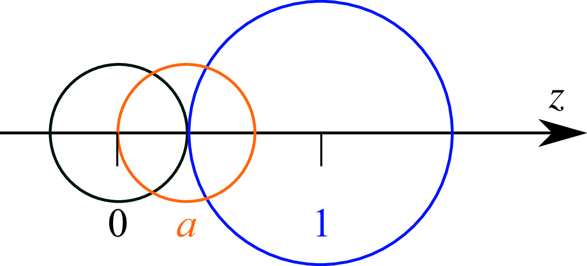
 z
 a∈R
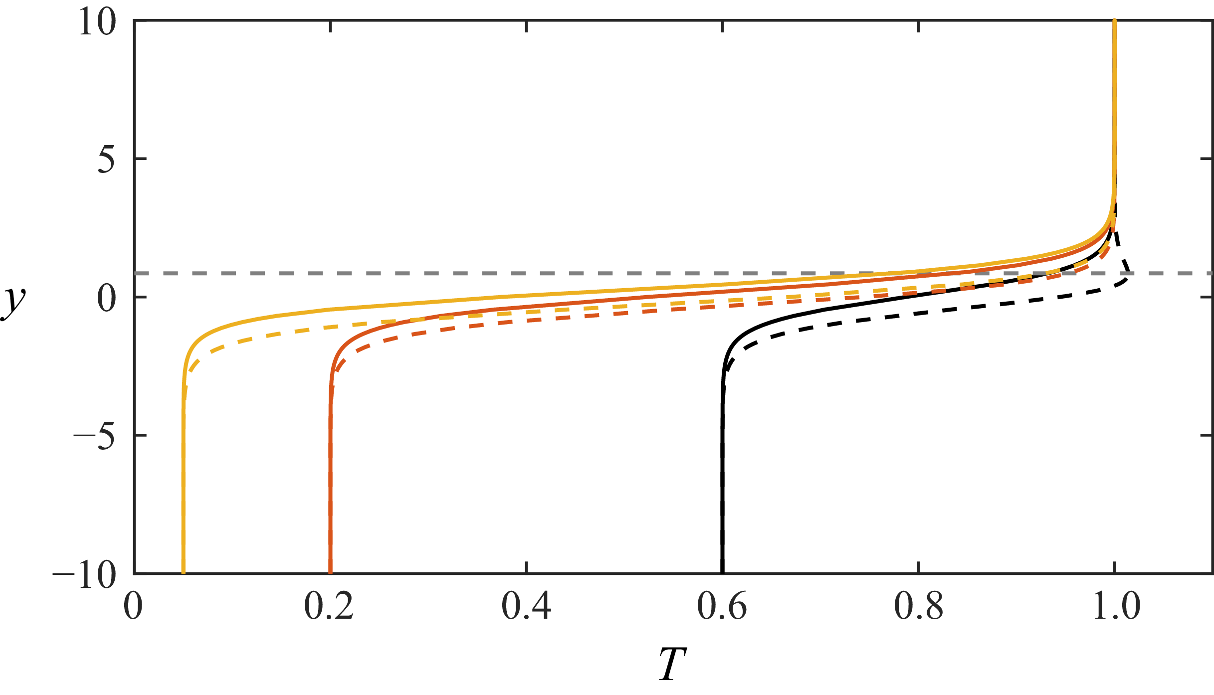
 M=1.7
 T~1=0.6
 T~1=0.2
 T~1=0.05
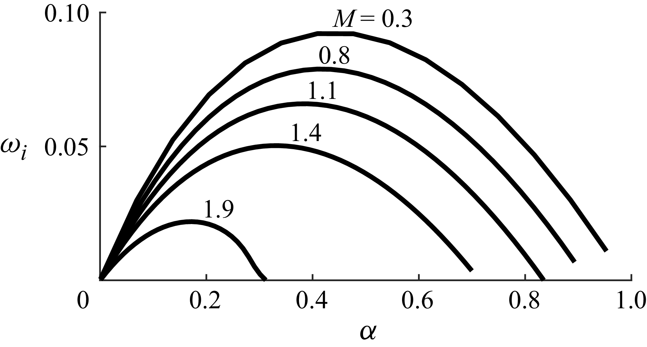
 ωi
 cx=ωr/α=0.5
 α

 ωi
 α
 cx
 ωi
 cx
 α
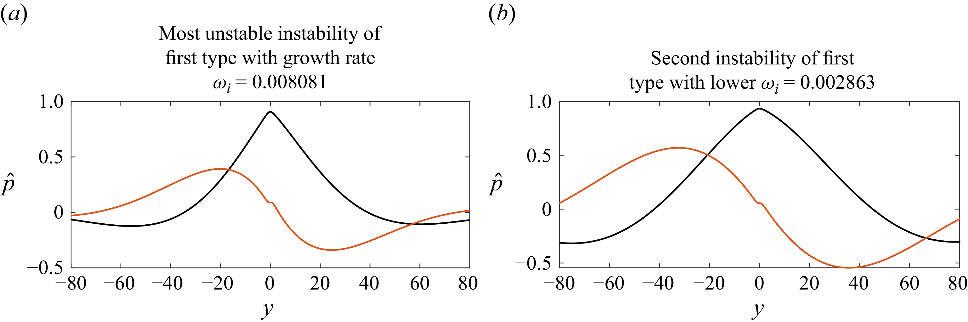
 M=2.23
 cx=0.5
 α=0.07061
 ωi=0.008081
 ωi=0.002863
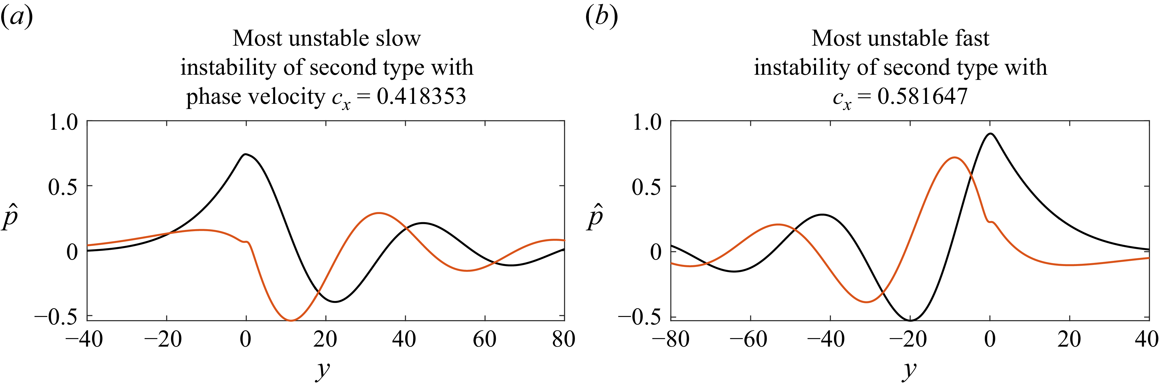
 M=2.23
 α=0.17
 ωi=0.00812868
 cx=0.418353
 cx=0.581647
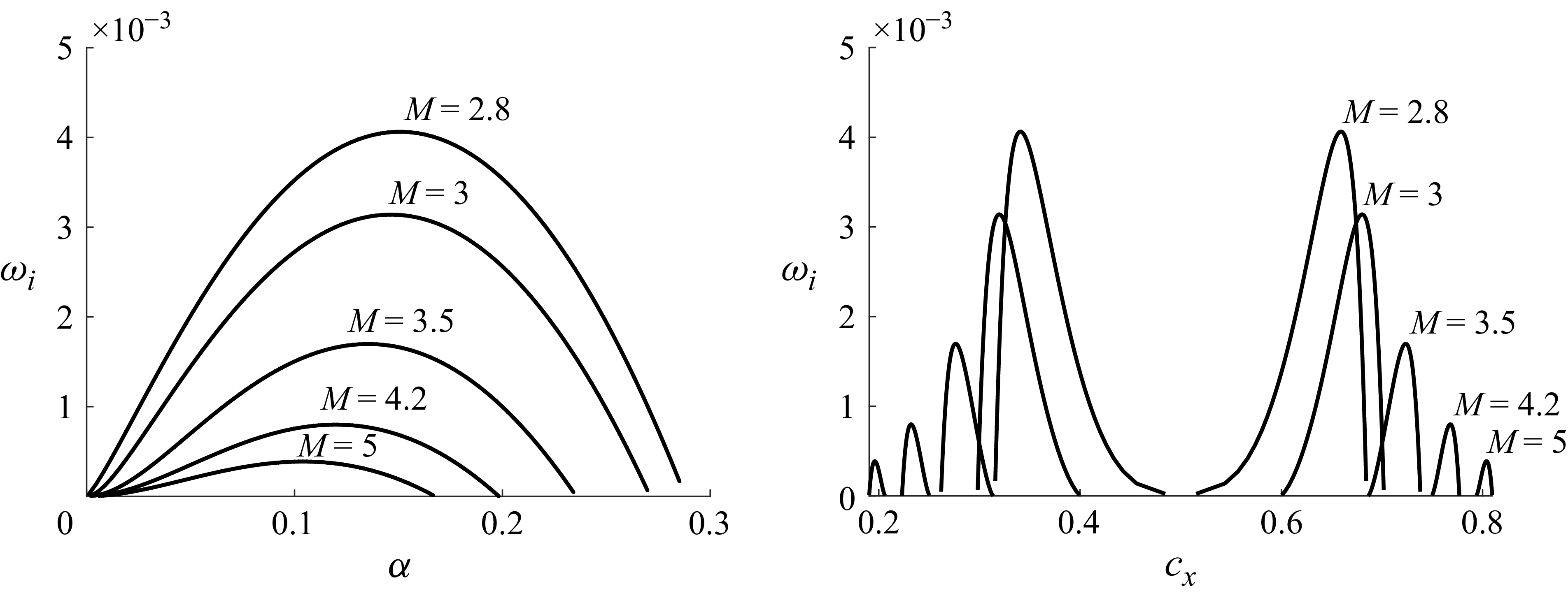
 ωi
 cx
 α
 cx=0.5

 ωi,3D
 β
 M3D
 β
 α3D

 ωi,T
 cx,T
 MT
 T~1

 Open access

