1. Introduction
The role of ice streams in the possible instability of the West Antarctic Ice Sheet, with implications for a possible rapid rise of worldwide sea level, is under current discussion (Reference AlleyAlley, 1990; Reference BindschadlerBindschadler, 1991; Reference MacAyealMacAyeal, 1992; Reference AlleyAlley and MacAyeal, 1994). In the ice streams, of width ∼50 km and length ∼400 km, the ice moves at speeds ∼10–100 times faster than in the ice sheet as a whole (Reference BentleyBentley, 1987; Reference Whillans, Bolzan and ShabtakWhillans, and others, 1987; Reference Bindschadler and ScambosBindschadler and Scambos, 1991; Reference Whillans and van der VeenWhillans and Van der Veen, 1993). To explain this anomalously rapid motion it has been proposed that the base of the ice is at the melting point and that the ice moves by rapid basal sliding (Reference RoseRose, 1979) or by rapid deformation of soft, water-saturated subglacial sediment (Reference Alley and MacAyeaLAlley and others, 1986, Reference Alley, Blankenship, Rooney and Bentley1987; Reference Blankenship, Bentley, Rooney and AlleyBlankenship and others, 1986, Reference Blankenship, Bentley, Rooney and Alley1987). The existence of basal melting and high basal water pressures, which would promote both basal sliding and soft-bed deformation, was demonstrated in boreholes drilled to the bottom of Ice Stream B (Reference Engelhardt, Humphrey, Kamb and FahnestockEngelhardt and others, 1990). In subsequent field-work we have endeavored to obtain observations of basal water pressure and transport that would deline the nature and functioning of a basal hydraulic System within which the high basal water pressure is generated, and that would permit its role in controlling the lubricating action involved in basal sliding and soft-bed deformation to be evaluated. T hat such control should be exercised by basal water has been indicated by observations in glaciers Reference KambKamb and others, 1985, p.474; Reference IkenIken and Bindschadler. 1986: Reference Boulton and HindmarshBoulton and Hindmarsh, 1987, fig. 7; Reference Kamb and EngelhardtKamb and Engelhardt, 1987, p. 34; Reference Kamb, Engelhardt, Fahnestock, Humphrey, Meier and StoneKamb and others, 1994) and by theory (Reference WeertmanWeertman, 1969; Reference IkenIken, 1981; Reference FowlerFowler, 1987; Reference AlleyAlley, 1989a, Reference Alleyb, Reference Alley1993; Reference KambKamb, 1991).
This paper presente our observations on basal water pressure and transport in Ice Stream B and an attempt to interpret them in terms of a model of the basal hydraulic system. As will be seen, different observations do not appear at first sight to conform to a single simple model. By introducing further complications we can achieve some resolution of the interpretive difficulties, but a fully satisfactory, complete model, well supported by observation, is a goal yet to be attained. However, we believe that the observations and provisional interpretations will be important, in combination with further observations in the future, for constraining the nature of the basal hydraulic system under the ice stream.
2. Observational Program
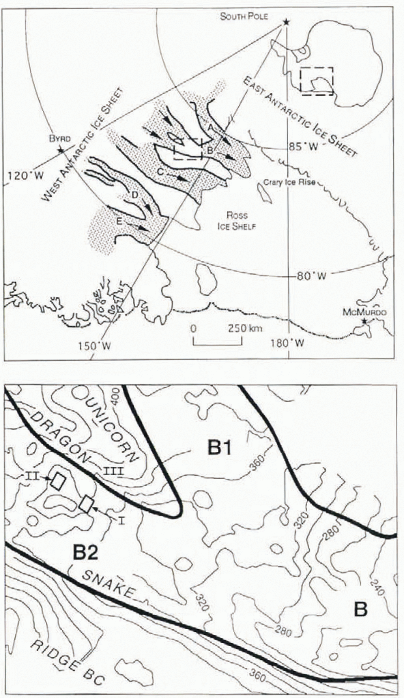
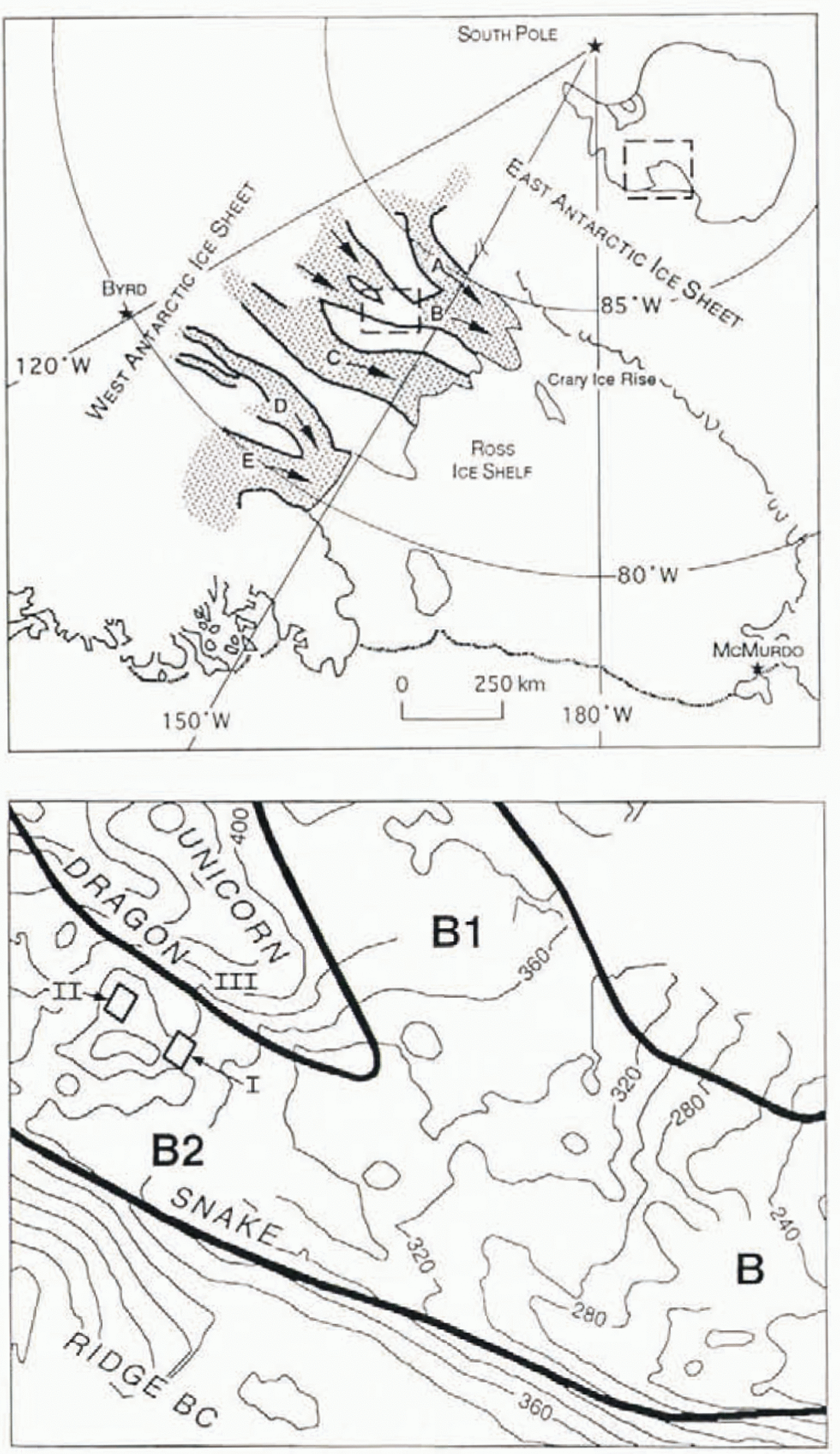
The borehole observations reported here were made in holes drilled to the bottom by hot-water jet drilling, in three site areas: (I) within 1km of old UpB camp (Upstream Bravo, here called UpB ’81, which in 1988 was located at 83°29.03′ S, 138°11.57′ W): (II) within 1 km of new UpB camp (here called UpB ’95, located in 1995 at 83°27.4′ S, 137°46.9′W), about 10 km east of the 1995 position of Up B ’84; and (III) within an area of ∼5 km dimension near 83°34.4′ S, 138°9.0′W on the Unicorn, the ridge between ice-stream branches B1 and B2. The site areas are indicated on the larger-scale map in Figure 1.
Location sketch maps. The upper panel shows West Antarctic ice streams A–E (shded) in relation to the Ross Ice Shelf and South Pole. The lower panel, from a surface elevation map by Reference PatersonRetzlaff and other (1993, fig.7), is an enlargement of the dashed rectangle in the upper panel. It shows the junction of tributary ice streams B1 and B2 to form the trunk ice stream B (flow from upper left to lower right). I, II and III indicate the three study areas of the present report. The reclangles indicte with some exaggeration the site areas covered by the maps in Figures 2 and 4. Te site of camp UpB ’95 in rectangle II (see Fig. 2). Marginal shear zones are shown with heavy lines (width not to scale) and labelled “Dragon” and “Snake” according to custom. The ridge between streams B1 and B2 is called the Unicorn.
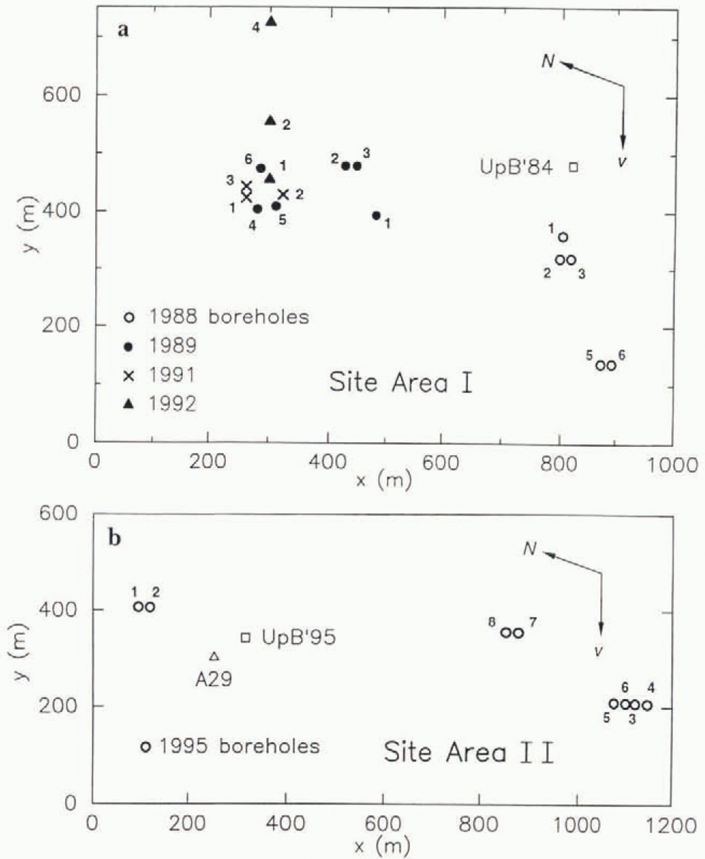
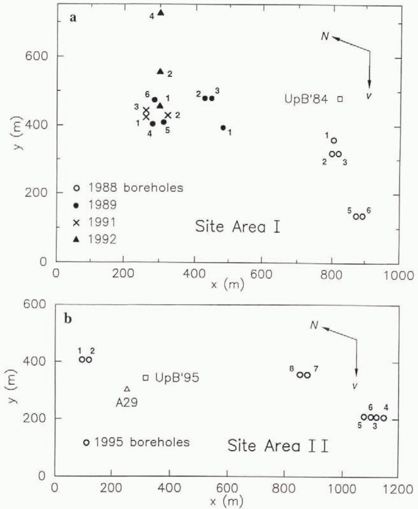
Detailed maps showing the locations and number designations of the individual boreholes drilled in she areas I and II are given in Figure 2. The boreholes are plotted in their positions relative to one another on the ice surface: relative to the bed below they were displaced 1.2 m d−1in the indicated flow direction, because of the ice-stream motion (Reference Whillans, Bolzan and ShabtakWhillans and Bolzan, 1987, Table 1). Borehole depths were in the range 1025–1057 m ( Table 1). The boreholes numbered with prefix 88- were drilled in field season 1988–89, those with prefix 89- in season 1989–90, and so on. The prefixes are omitted in Figure 2, where their place is taken by the plotted borehole location symbols.
Maps of borehole locatiom (a) in site area land (b) in site area II. Borehole year (1988 to 1995; see text) is indicated by the location symbol type (see keys), and borehole number within each year is indicated by the number alongside each location symbol. Site area II is located approximately 10 km upstream form site area I (see Fig. 1). The arrows labelled v show the flow directon; N is nrth. Location of camps UpB ’84 and UpB ’95 are shown with open squares. The open triangle shows the location of pole A29 in the marker-pole grid of Ohio State University (Reference WhillansWhillans, 1984, fig.2). Origin of the x,y local coordinate systems is arbitrary.
Most of the observational data presented in this paper consist of records of water pressure (rarely, ice pressure) obtained with pressure transducers of the Paine Instrument Co. (Seatlle), type 212. For observations of the waterlevel in open boreholes we generally use pressure transducers of fullscale rating 200psi (1.38 MPa) placed at a depth of 100–120 m beneath the surface, just above the well pump used for recycling the drilling water. The well pump and pressure transducer are placed in an auxiliary hole 120 m deep, located only 0.25 m laterally from the center of the main hole. In the course of drilling, the auxiliary hole soon becomes connected laterally to the main hole by melting of the hole walls because of heat introduced into the main hole for drilling and into the auxiliary hole lo keep the well pump from getting frozen in; the lateral connection is shown by the fact that the well pump does not draw the water level in the auxiliary hole down to the level of the pump, as it would do in an unconnected hole. For spot checks of the water level and for calibration of the pressure transducers, a sounding float is used.
For long-term records of basal water pressure, we use pressure transducers of full-scale rating 2000 psi (13.8 MPa), placed at the bottom. Each transducer is mounted in a pressure-tight case of outside diameter 5.1 cm and length 60 cm, with the access port for pressurized water located at the bottom. The transducer case is suspended on a steel-armored four-conductor able (Amergraph cable) through which the transducer is powered (12 or 28 V DC) and its output signal (0–3 or 5 V) transmitted to the surface. The bottom of the transducer case is placed as close as possible to the bottom of the borehole, without slack in the cable; this can generaliy be done to an accuracy of ±0.5m. After 1 or 2 d the hole has frozen up enough that the cable is frozen to the borehole wall and can no longer be raised. Such transducer installations have proven notably robust. The one installed in borehole 88–3 in December 1988 went dead in January 1992 after operating for 4 years. The unes in holes 89–4 and 91–1 were still operating normally in December 1995,6 and 4 years after installation, respectively.
3. Initial Basal Water Pressure
When a hole is bored by hot-water drilling at sites I and II, in the ice stream, the water in the hole almost always behaves in the following way. As drilling progresses, the water level in the hole remains high normally at depth 20–30 m below the surface), and then, when the drill comes to a stop at the bottom of the ice, the water level drops rapidly to depths of about 100–115 m. We refer to this drop as “breakthrough” to the basal water conduit system—the system that receives the water that drains from the hole during the breakthrough event.
The downrush of water in the borehole upon breakthrough throws a heavy load onto the drill stem, which is delected by a load cell that monitors the tension in the drilling hose at the surface. Sometimes the drill stem (a heavy brass cylinder with the drill jet nozzle at the bottom) is pulled down so forcefully that it becomes jammed at the bottom of the hole and can be recovered only with difficulty. Because of this pull-down it is often difficult to detect that the drill advance ceases essentially at the moment of breakthrough, but attempts to drill into the bottom after breakthrough always show that the drill advance is very slow or nil, and piston coring shows that the material below the bottom of the hole is unfrozen, water-saturated till. The lithological characteristics of this till are presented in a separate paper (unpublished information from S. Tulaczvk and others).
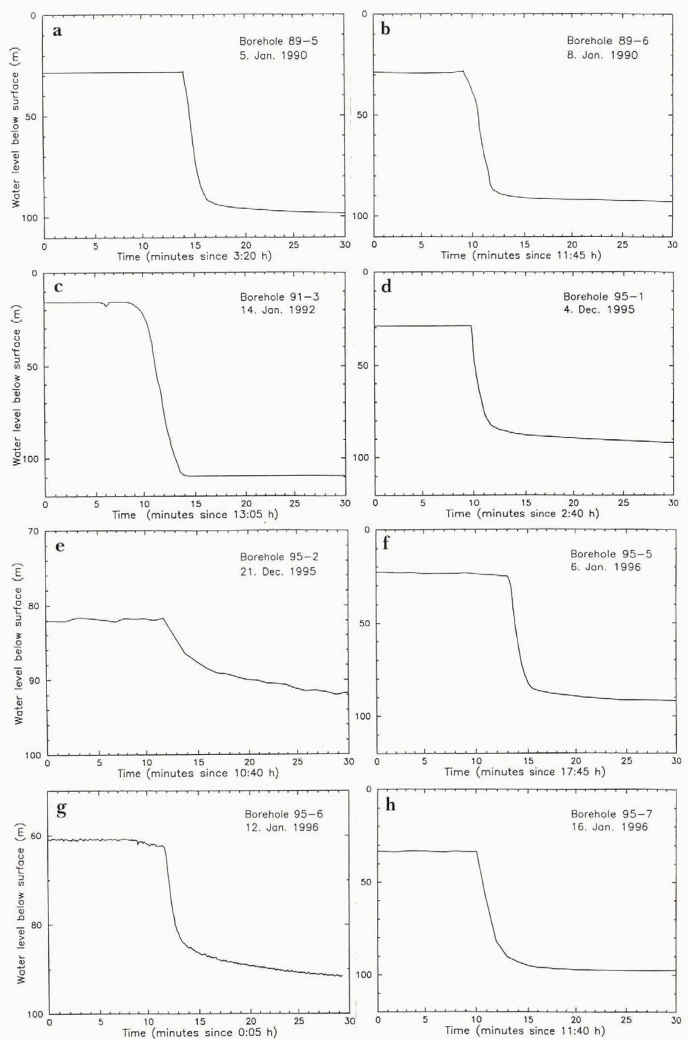
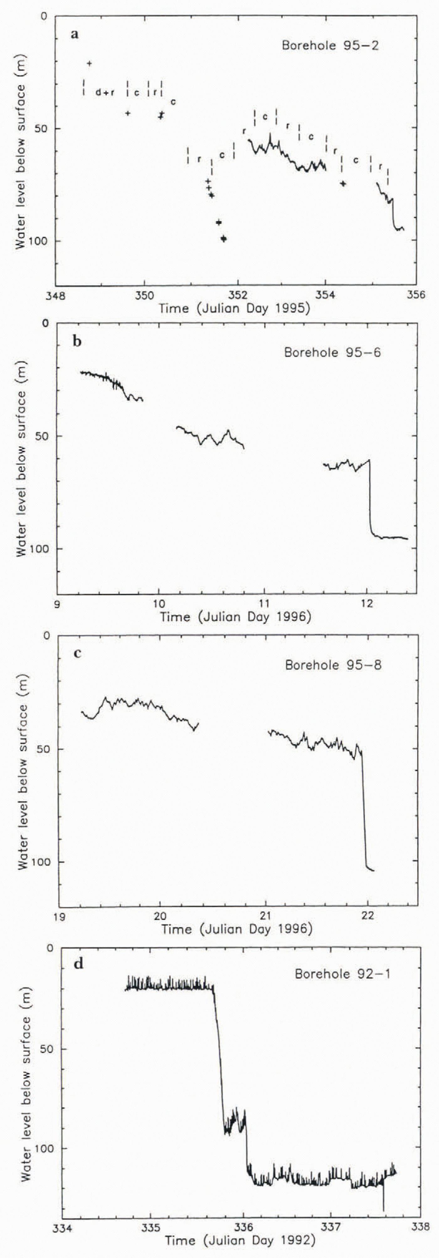
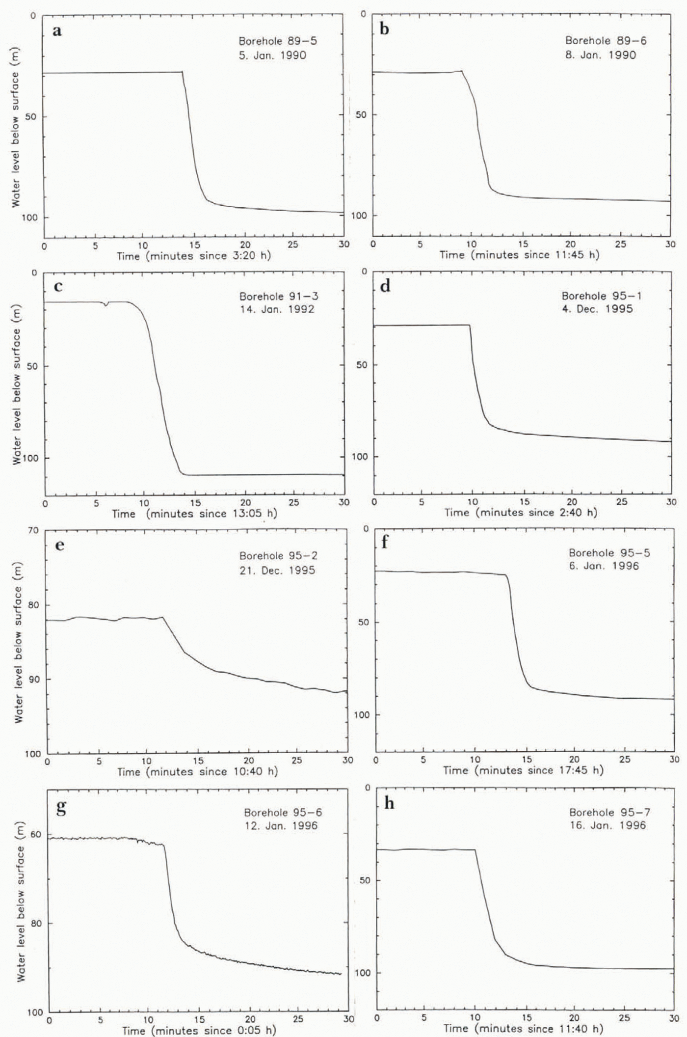
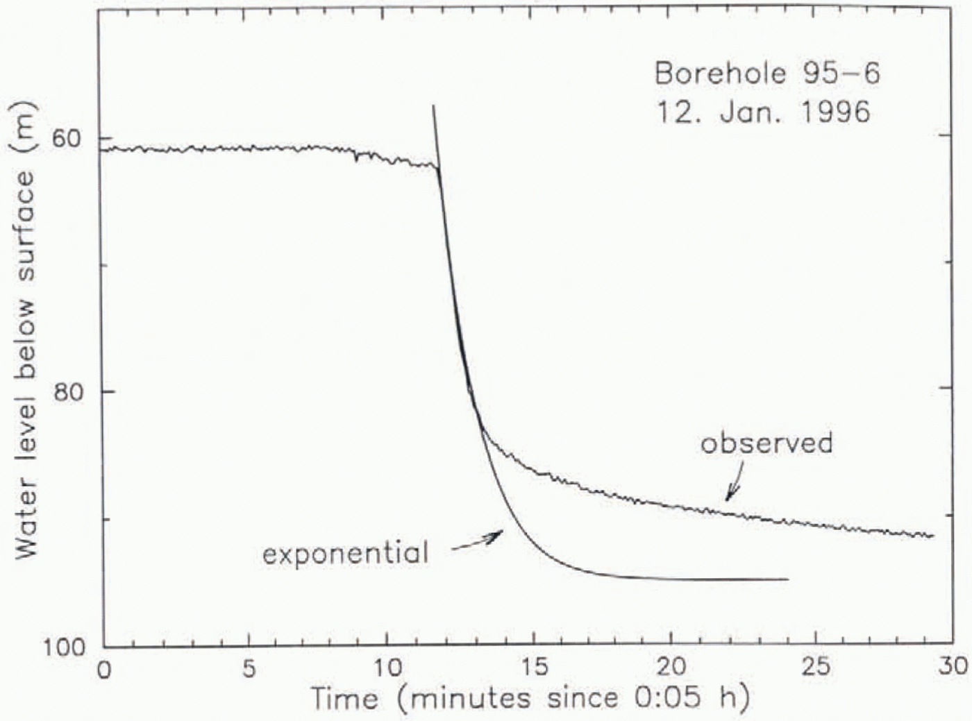
Measured graphs of borehole water level vs time during drilling and breakthrough are given in Figure 3. The drop in water level on breakthrough is approximately exponential in time, and the “drop lime” — the time for completion of about 90% of the total drop — is in the range 2–7 min (values in Table 1). These results are similar to those from a borehole in Trapridge Glacier, Canada, given by Reference Stone and ClarkeStone and Clarke (1993, Fig. 4), except that for the latter the drop time was only about 20 s.
Borehole water level vs time for eight boreholes, showing water-level drop on breakthrough to the basal water system. The borehole numberand breakthrough date are identified in the upper right corner of each frame.
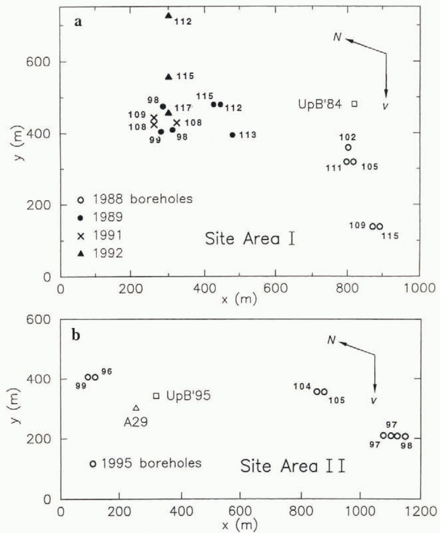
Initial borehole water level after completion of breakthrough, in meters below the surface, written alongside the location symbol for each borehole, plotted as in Figure 2.

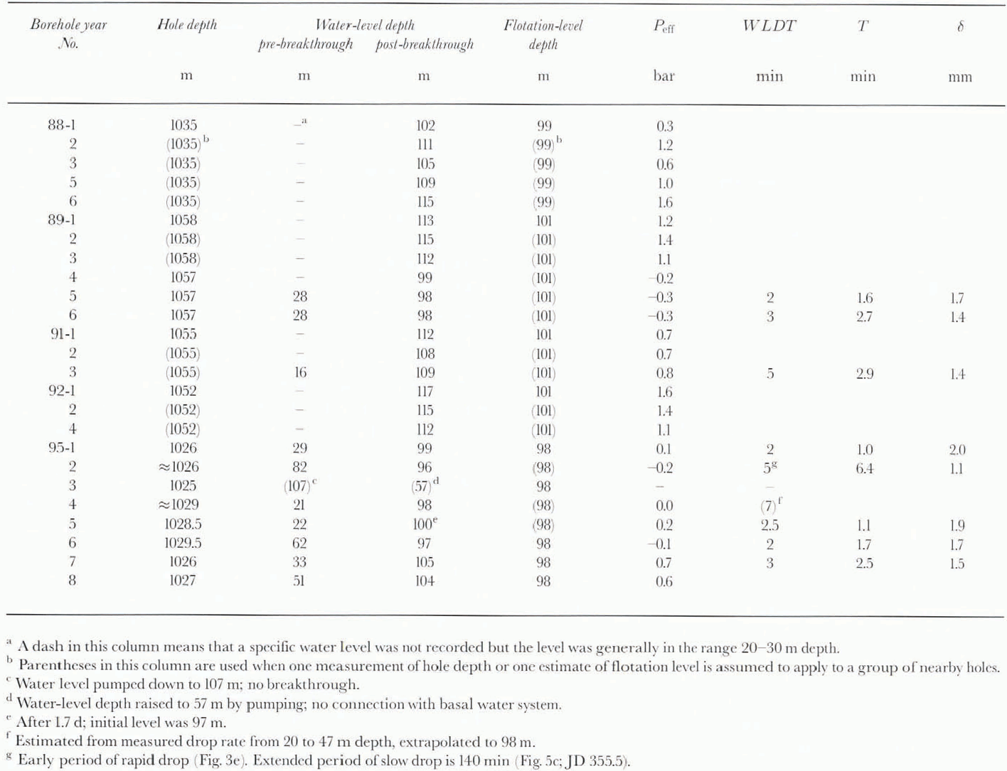
Boreholes in Ice Stream B near UpB ’84 and UpB ’95: water-level depth before and after breakthrough; flotation level and basal effective pressure Peff; water-level drop time (WLDT) and time constant T; gap-conduit width δ
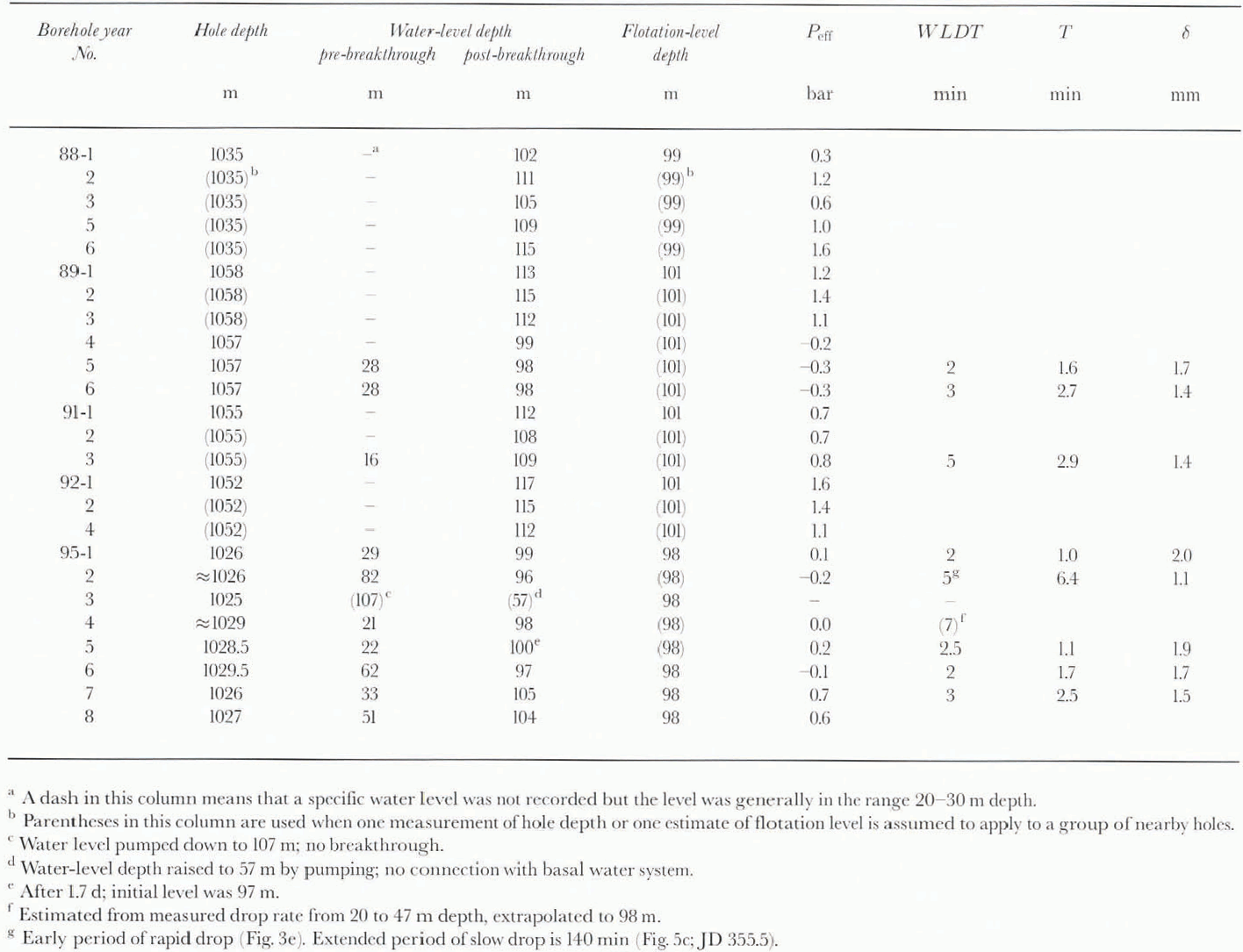
Within an hour or so after breakthrough the water level reaches an essentially steady depth, here called the “initial post-breakthrough water level”, or “initial level” for short. The water level is a measure of the basal water pressure in the basal water system to which the borehole has become connected in breakthrough. All available initial water-level depths, measured with a pressure transducer as noted above, or sometimes with a sounding float, are listed in Table 1(conservatively estimated error ±1 m). They are in the depth range 96–117 m. The values are given as water-level depths below the surface rather than as basal water pressures, for reasons explained in section 4, where the conversion between the two is stated. The relation of basal water pressure to ice overburden pressure can be expressed in terms of the relation between the water level and the flotation level, the water level that corresponds to the ice overburden pressure at the base of the ice. Flotation levels at the various boreholes are estimated in section 4 and are listed in Table 1. They range from 98 to 101 m (ଁ3 m). Most of the initial water levels are near but definitely deeper, by 3–16m, than the estimated flotation level; the corresponding basal effective pressure ice overburden pressure minus basal water pressure) is in the range +0.3 to + 1.6 bar ( Table 1). Five initial water levels are at depths shallower than the estimated flotation level by up m 3m, corresponding to a basal effective pressure that is as much as 0.3 bar negative. Since a negative basal effective pressure is not possible in a steady-state glacial system, the water levels that appear to give negative effective pressure either involve data error or indicate anomalous conditions in the basal water system.
The variation of initial water level from hole to hole, ranging over depths from 97 to 117 m ( Table 1). is noteworthy: The spatial pattern of variation can be assessed from Figure 4, in which the initial water-level depth at each borehole is indicated alongside the map localion of the hole. Boreholes in clusters up to ∼100 m in dimension, and drilled in close succession so that the effect of time variations (section 5) is minimized, have similar initial water levels, within 2 or 3 m, whereas more distant holes, or holes in the same cluster but drilled in different field seasons, often diller in initial level by 5–10 m. This suggests that the water levels sample basal water pressure over areas of up to about 100 m in dimension. Holes 88–1 to 88–6 deviate from this pattern in having a more random spatial distribution of water-level variations. The variations in basal water pressure implied by the variations of the water level, although small in comparison to the basal water pressure itself (1.5 vs 95 bar), are large percentagewise when expressed in terms of basal effective pressure, which varies from ∼0 to 1.6 bar. The variations are significant in relation to the nature of the basal water system (sec interpretation in section 9d).
There are a few ways in which borehole water levels sometimes depart from the behavior described above:
If borehole drilling operations continue for several days prior to breakthrough, as is normal when ice-core drilling is done, the water level gradually gets drawn down below the normal high level prior to breakthrough. Examples are shown in Figure 5. This is due not to leakage of water from the borehole, but to the way drill operators tent to avoid providing make-up water to the drilling system, which requires the laborious effort of quarrying snow blocks for melting; thus, as shown in Figure 5a, during reaming (which uses up water) the water level tends to fall, while during coring (which uses little water) it tends to rise. An exception that may represent leakage is the more rapid drawdown recorded in Figure 5a during Julian day (JD) 351.3–351.7.
Examples of drawdown of the borehole water level prior to breakthrough. In (a), the time intervals marked “c” are when ice coring was being done, and those marked “r” are when reaming was being done, which uses more watet than coring does, “d+r” includes the initial drilling and reaming of the hole. In (d). the rapid drawdown during JD 335.67–335.79 was produced by a pumping-out test (section 6). In (a), (b) and (c). breakthrough occurs near the end of the record; in (d) it occurs at 0000 h on JD 336.

In the drilling of boreholes outside the ice stream (site-area III; see Fig. 1), the drill comes to a stop without the occurrence of any breakthrough, the borehole water level remaining high. Thermistor measurements (to be reported in a separate paper) show that at the bottom of the borehole the temperature is below freezing by 1 or 2°C The drill is stopped by rock debris that is so abundant and/or contains such large clasts that it cannot be melted out from the ice and penetrated at an appreciable rate by the hot-water jet drill. Samples of this rock debris, melted loose and settled out at the bottom of the hole, have been obtained by piston coring and studied sedimentologically (unpublished information from S. Tulaczyk and others).
Borehole 95–3 behaved in a manner similar to holes outside the ice stream. We infer that at site 95–3 a layer of frozen till intervened between the base of the penetrable ice and the melting isotherm below. This singular occurrence is spatially limited by normally behaving boreholes 3.5 and 7.4 m away (holes 95–4 and 95–6; see Fig. 2b). Further aspects of the singular behavior of hole 95–3 are discussed in section 6.
One borehole (88–2) did not experience an immediate breakthrough and water-level drop on reaching the bottom as indicated by cessation of drill advance, but 9 h later the water level dropped to 111 m, a normal initial depth. This may be a case that started out like hole 95–3 but in which subsequent development of a spontaneous fracture through the underlying frozen till gave breakthrough to the basal water system. By 25.5 h later the water level had risen to 43m, indicating that connection to the basal water system had already closed up and suggesting that the connection was weak in the first place. The scarcity of boreholes that connect to the basal water system only after a marked delay or not at all is in strong contrast with the situation in temperate glaciers, where many boreholes connect only after several days and often not at all (e.g. Reference HodgeHodge, 1979: Reference Kamb and EngelhardtKamb and Engelhardt, 1987, p. 34).
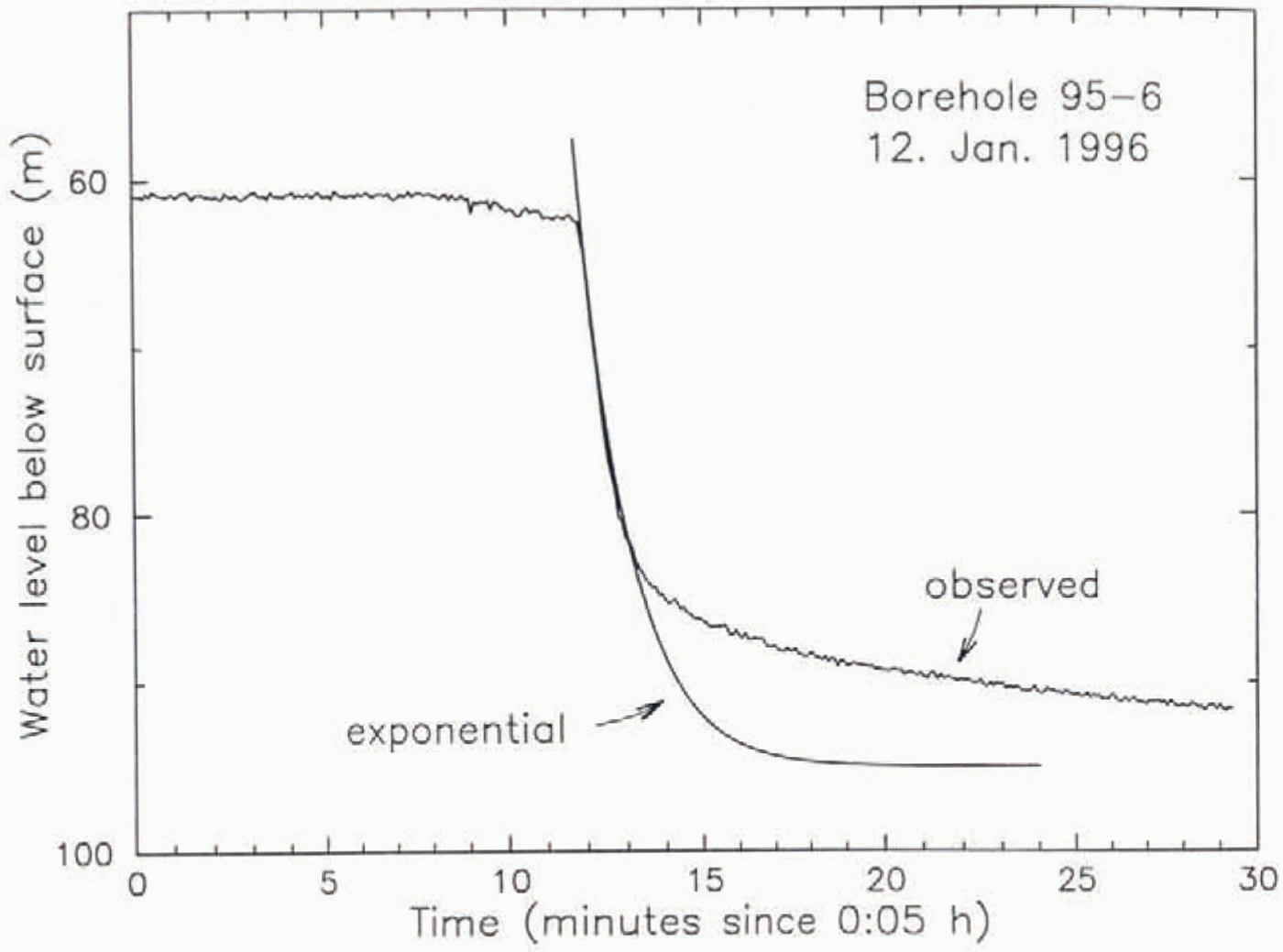
Although the drop in water level on breakthrough is to some approximation exponential in time (Fig. 3), a number of distinct departures from exponential form have been observed: (1) The onset of the drop is usually abrupt, but in one case it was gradual (Fig. 3c). (2) In several cases of abrupt onset, the drop rate was most rapid not at onset but instead a short time later: this is especially evident in Figure 3b, but can also be seen in Figure 3f, and perhaps Figure 3aand d. (3) In one instance there was a small pre-breakthrough drop, followed quickly by recovery (Fig. 3c). (4 )The size of the “tail” part of the drop curve is not always in the correct exponential proportion to the initial, main part of the drop; Figure 3cis an example of very little tail, while Figure 3cand g are examples in which the tail is overly large. This is demonstrated in Figure 6, where an exponential curve has been fitted to the main initial drop in the curve of Figure 3g, with an asymptotic post-breakthrough depth of 95 m, which is slightly above the 97 m depth indicated by later water-level data ( Table 1). A similar discrepancy between a theoretical (modeled) curve and an observed water-level-drop curve Brorn a borehole in Trapridge Glacier, Canada, is shown by Reference Stone and ClarkeStone and Clarke (1993, Fig. 4). The extreme constancy of the water level in Figure 3cafter time 14 min is due to the water level having fallen below the depth of the measuring pressure transducer at that time.
Comparison between the curve of water-level drop on breakthrough in borehole 95–6 and an exponential z0(t) = zo(0) exp(−t/T), where zo(t) is the borehole water-column height above the post-breakthrough level (taken to be at depth 95 m, so Zo(0) = −(63–95) = 32 m). Time t is relative to the start of the breakthrough at 11.9 min on the abscissa scale of the plot. The time constant T = 1.7 min is adjusted to make the exponential fit the main initial part of the observed curve.
4. Flotation Level
The following method is used for estimating the flotation levels in Table 1, from which the effective pressure at the bottom in each borehole is obtained. The firn/ice density down to a depth of 47 m in site area I has been measured by Reference Alley and BentleyAlley and Bentley (1988, Fig. 4). Below that depth we use the density-depth data obtained by Reference GowGow (1970)from the Byrd borehole, in the West Antarctic ice sheet some 490 km from site I. Because the two sets of density-depth data do not connect smoothly across the data gap from 47 to 80m depth, a smooth connection to the data point at 47 is forced by linearly interpolating between data points at 17 and 137 m. Using a thermal-expansion coefficient of 1.5 × 10 −4K−1, the measured densities are corrected for thermal expansion/contraction between the temperature of original measurement and the temperature at depth in the ice sheet at UpB ’84 {Reference Engelhardt, Humphrey, Kamb and FahnestockEngelhardt and others, 1990, Fig. 2, and unpublished data). (The temperature of original measurement by Reference Alley and BentleyAlley and Bentley (1988)is assumed to be −5°C For Gow’s data it is taken to be the temperature −28.7°C in Reference GowGow (1970, Fig. 4), since the densities there given were corrected for this in situ temperature. The densities are also corrected to the in situ pressure at depth, using a compressibility of 1.3 × 10⁻⁵bar−1. The corrected densities are integrated with depth from the surface to the bottom, to obtain the overburden pressure and the height of a water column producing the same pressure, taking into consideration the compressibility of water (5.1 × 10⁻⁵bar−1). The flotation-level depth is then the difference between the ice thickness (borehole depth) and the water-column height. For a borehole 1035 m deep the temperature correction to the flotation-level depth is + 1.5 m and the pressure correction is +1.7 m, so that without these corrections the calculated flotalion level would be at 95.8 m depth rather than 99 m as given in Table 1. This gives some idea of the possible errors that may enter the calculation of the flotation level. The largest uncertainty, however, is doubtless in the assumption that the ice densities from the Byrd core are applicable at UpB.
We present the pressure data mainly in terms of equivalent water levels and flotation levels for several reasons: (1) Some of the measurements are made with a sounding float, which gives water levels directly. (2) The pressure transducers used to measure water levels are placed at a known depth (near 110 m) and are calibrated on the basis of water-level measurements made with the sounding float; the results are therefore closer to direct floal measurements than to measurements of water pressure at depth. (3) For a borehole not in connection with the basal water system, Water level can be measured and reported, but basal water pressure cannot. (4) Water-level elevation is the same as hydraulic head, which is of direct importance for flow in the basal water system. (5) Reporting borehole water levels is standard practice (e.g. Reference MeierMeier and others, 1994).
Conversion of a water-level depth dwto a basal water pressure in ice of thickness PBWis done as follows. The equivalent water column is hw= h1− dw, and the pressure is P Bw= ρ wgh w[1 + (β wρ wgh w/2)], where βwis the compressibility of water (5.1 × 10⁻⁵bar−1) and ρwis the density of water at atmospheric pressure, The term involving βwis a correction for change of density with pressure, related to the pressure correction involved in calculating the flotation level dFConversion of flotation level to basal overburden pressure is the same, with dWhaving the particular value df.
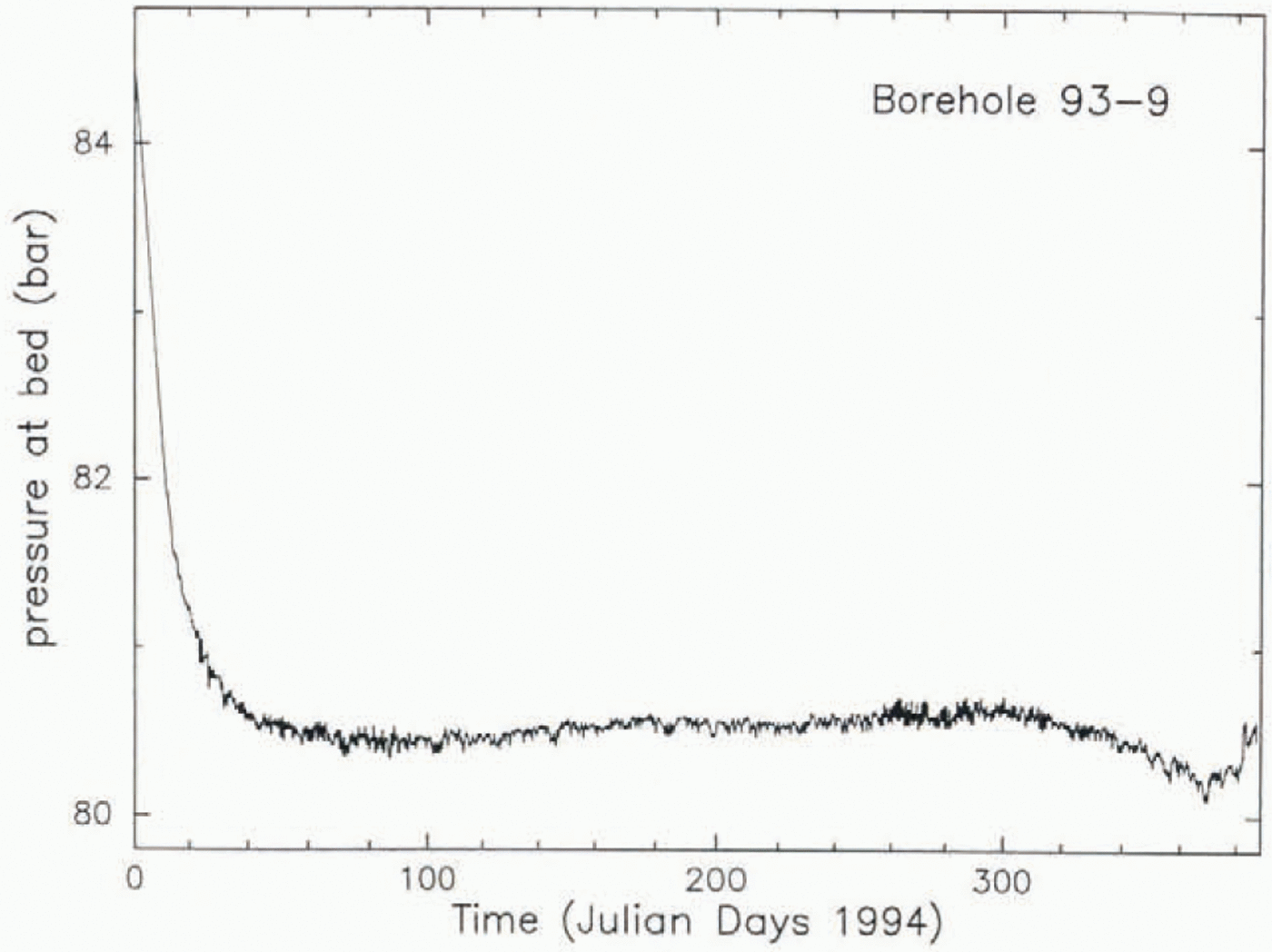
An observational check on the flotation-level calculation above can be made for borehole 93–9, in which the over-burden pressure was measured (Fig. 7). The borehole is in site area III. where there was no basal melting and therefore no possibility that basal water pressure was involved. The pressure-transducer instrument was suspended 1 m above the bottom of the borehole and was encased in a fluid-tight plastic sack filled with antifreeze (ethylene glycol) so that the pressure brought to bear on the sack by the inclosing ice would be transmitted via the fluid to the pressure-access port of the transducer. When the initial pressure transient had run its course the measured pressure settled down to 80.5 bar. In the ensuing 300 d the measured pressure rose gradually to 80.7 bar and then decreased to 80.2 bar (Fig. 7). The overburden pressure calculated by the foregoing method for this borehole (of depth 911 m) is 80.8 bar. The agreement between measured and calculated overburden pressure is within 0.2–0.6 bar (corresponding to 2–6 m in flotation level).
Ice pressure reported by a pressure transducer at the bottom of borehole 93–9, in site area III (on the Unicorn; Fig. 1). After the initial transient due to borehole freeze-up, the pressure reported is the ice overburden pressure (section 4). The borehole depth was 911 m.
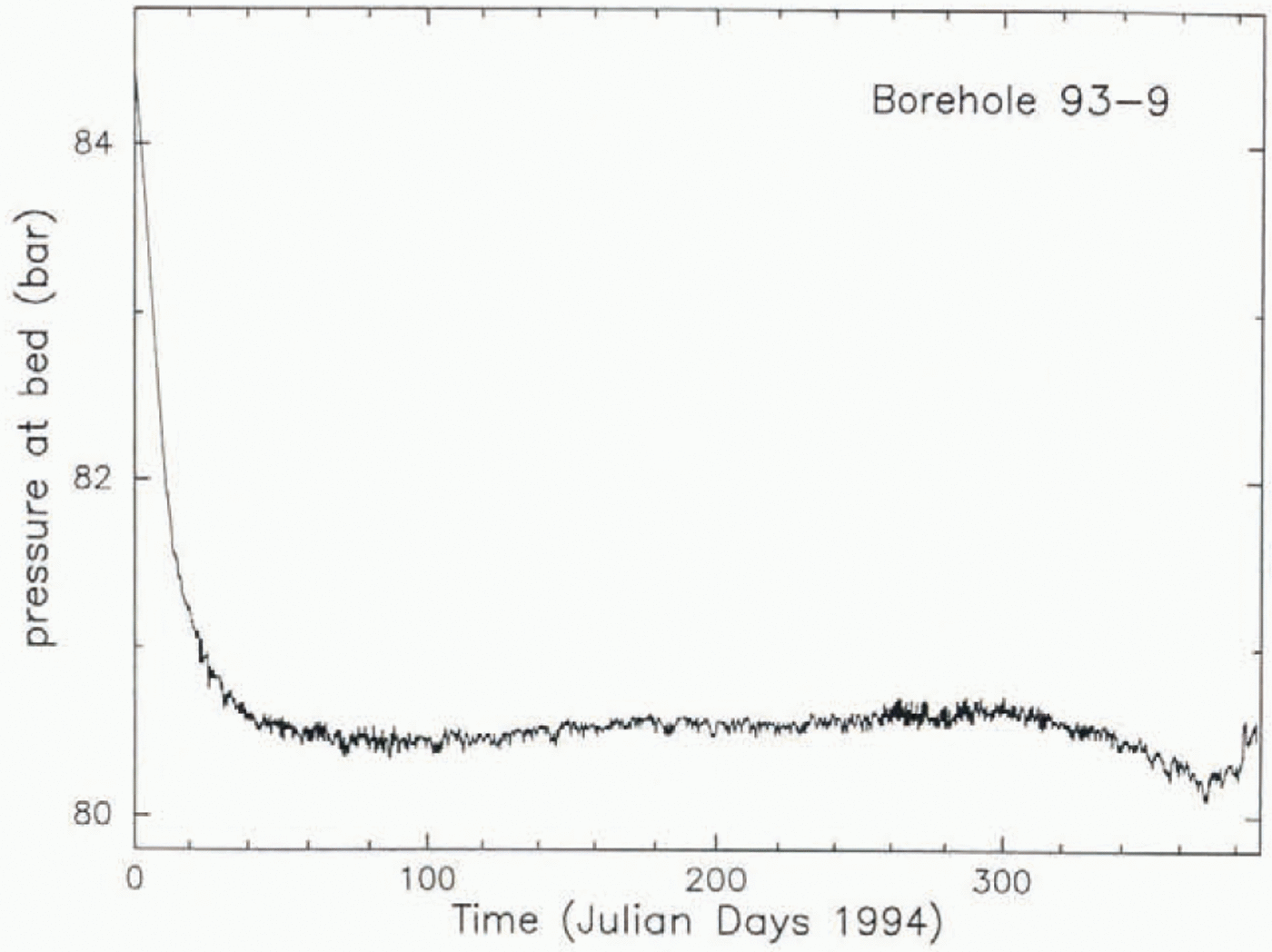
The cause of the variation in measured pressure in hole 93–9, corresponding m a 5 m fluctuation in water level, is not known, except for the initial transient that is presumably caused by the freeze-up of the initially water-filled borehole.
The slightexcess of calculated overburden pressure over measured pressure at hole 93–9 suggests that the calculation tends to give flolation-level depths that are too shallow, but the presence in Table 1of five negative values of basal effective pressure suggests instead that the tendency is to give flotation levels that are too deep by up m 3 m. The physical constraint requiring non-negative basal effective pressure is more powerful than any reasoning about the accuracy of the calculation and indicates that there are errors in calculated flotation level of as much as 3 m. The foregoing considerations suggest that we may be justified in placing an error figure of ±3 m on the estimated flotation levels.
5. Time Variation of Basal Water Pressure
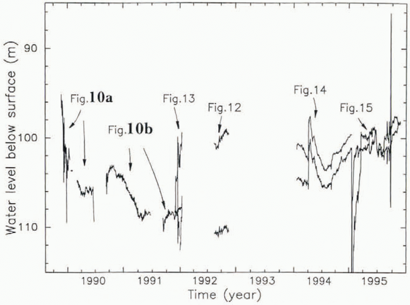
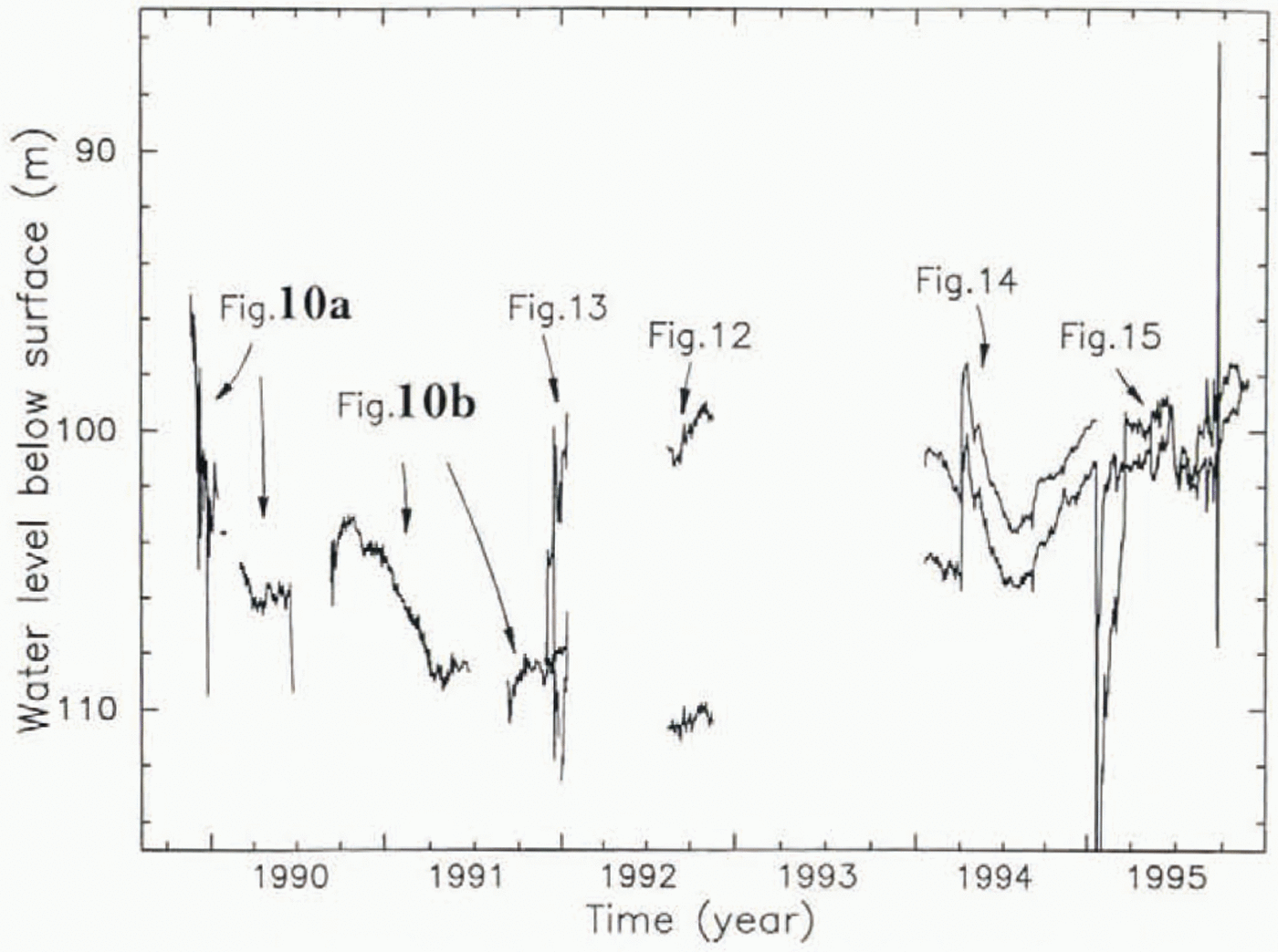
The basal pressure sensed by a pressure transducer placed at the bottom of a borehole in the ice stream does not remain steady at the initial post-breakthrough value but varies with time in complicated ways. The complete set of such data is given in Figure 8. with a much compressed time axis, and portions as indicated are shown with expanded time-scales in Figures 9–15. (Figure 9is outside the window of Figure 8.) The data come from pressure transducers installed in boreholes 88–3, 89–1 and 91–1, whose locations are shown in Figure 2a. The data gaps in Figure 8are due to malfunctions of power supply and/or data-recording system due mostly to winter cold. In presenting the data we continue to express basal pressure in terms of water level (section 4), even though there is no free water surface once the boreholes refreeze. Use of water level is consistent with the fact that prior to freeze-up each pressure transducer was calibrated by immersion in a water column of known height in the borehole, the height being known from sounding-float measurement of water level combined with measurement of pressure-transducer depth with the steel-armored pressure-transducer cable.
Measured basal water pressures over the 6 year period 1990–5. The arrows refer to the figures that give expanded plots ofparts of the complete record as indicated and that identify whick boreholes are the sources of the various traces shown.
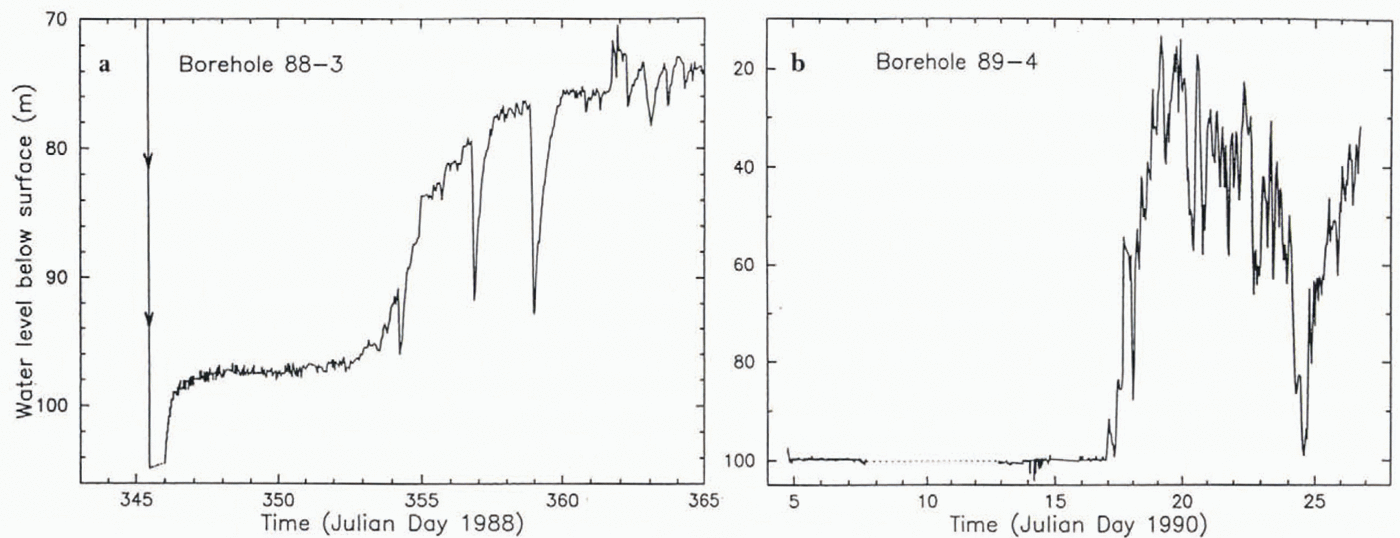
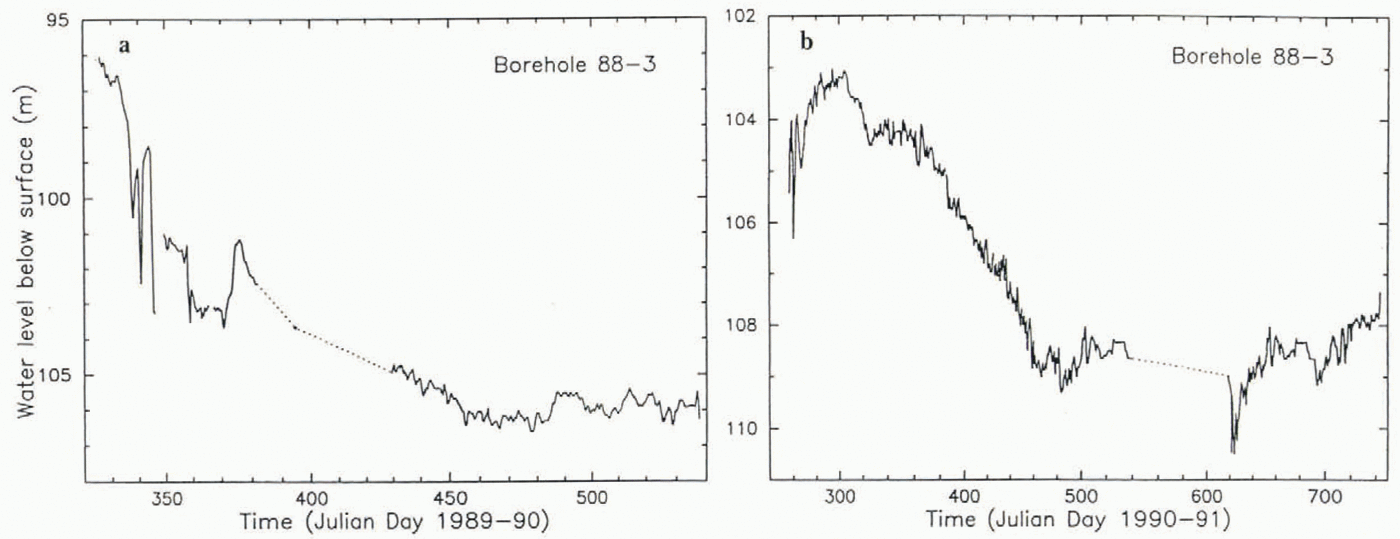
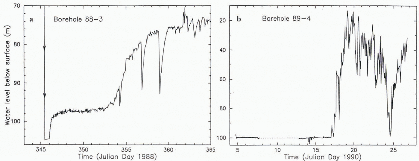
In borehole 88–3 (Fig. 9a) the rise of 6 m in water level, ∼16 h after breakthrough, took place on a time-scale that we expect for freeze-in of the cold upper part of the borehole, which should tend to raise the pressure in the inclosed water column that remains in the lower, more slowly freezing part of the hole. This type of pressure rise was observed by Reference Waddington and ClarkeWaddington and Clarke (1995, figs 8 and 9)in unconnected and blind boreholes in Trapridge Glacier, Canada; the time-scale of the rise (≈2−3h) is shorter than the time-scale ∼1 d seen in our Figure 9a. In order for the water pressure to rise, there must be an appreciable impedance in the basal water system or in the borehole’s connection to that system. The much larger rise that occurred 7–15d after breakthrough, to a level of about 72 m, far above flotation, must represent isolation of the pressure transducer from the basal water system, probably by ice forming over the pressure access port of the transducer. The spike-like sharp drops in pressure may indicate that the ice plug closing the access port was fractured occasionally as pressure built up inside the port due to freezing. (Similar sharp drops in pressure have been observed in Trapridge Glacier (Reference Waddington and ClarkeWaddington and Clarke, 1995, figs 1c and 7) and attributed to ice fracturing.) A more extreme case of such a pressure rise, to the even more extreme level of about 20 m, occurred in hole 89–4 in the period 17–19d after breakthrough (Fig. 9b). On the other hand, 91–1 showed only a small pressure rise, remaining below flotation (Fig. 10). The ending of the periods of excessive pressure — by about 1 year after breakthrough in hole 88–3 and by at most 2 years in hole 89–4 — can be attributed to melting out of the access port, presumably as a result of the basal melting that takes place under the ice stream.
Pressure records from boreholes 88–3 (a) and 89–4 (b) during the first 20 d after breakthrough. These records are not shown in Figure 9, because (a) falls before the time window of Figure 8 and because most of (b) would plot off scale.
Once the early post-breakthrough period of excessive pressure : (if any) came to an end, the pressure decreased to normal levels in the water-level range 98–112 m. Fluctuations within this range took place on a wide range of amplitudes and time-scales during the 6 year period represented in Figure 8. The character of the fluctuations is documented in Figures 10–15, which contain enlargements of parts of the record in Figure 8. The record from borehole 93–9 (Fig. 7), representing ice overburden pressure, which is presumably a nearly constant quantity (slightly varying due to accumulation of snow, ablation by wind, and the effect of vertical strain), suggests that there is inherent high-frequency “system noise” of amplitude 0.1 or 0.2 bar (1 or 2 m w.e.) and long-term apparent drift of up to about 0.5 bar (5m of water), disregarding the large initial transient. If these numbers are applicable to the other pressure-transducer installations, which measure basal water pressure, then only the larger variations seen in Figures 8–15 can be relied upon as real variations in basal water pressure. However, the possibility of system drift is made unlikely by the lack of a consistent correlation of apparent basal water-pressure variation with the seasonal surface temperature variation, which would seem to be the largest potential cause of system drift.
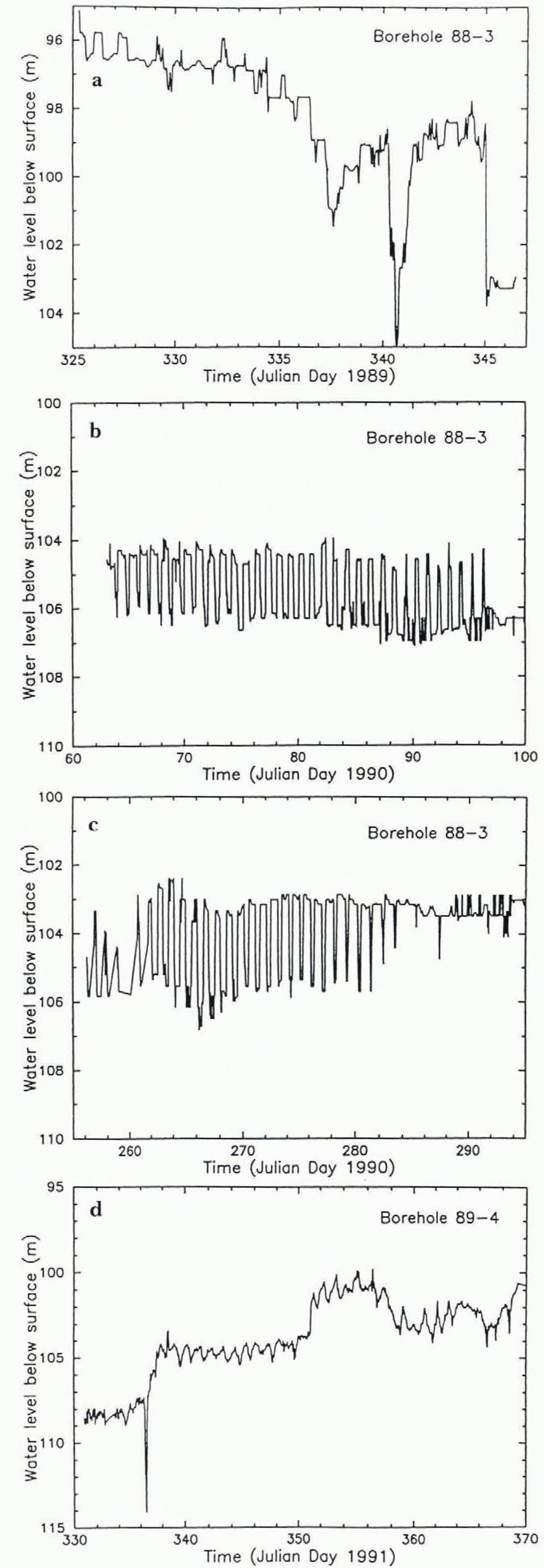
In some parts of the record there are conspicuous diurnal fluctuations (Figs 12 and 13). These do not appear to be artifacts caused by a temperature effect on the electronic sensing and recording systems, because some of the diurnal pressure fluctuations do not occur during the spring/summer field season when the diurnal temperature variation is large and when most of the electronics are at or near the surface for servicing and data retrieval. Reference Harrison, Echelmeyer and EngelhardtHarrison and others (1993)called attention to these fluctuations (in relation to diurnal fluctuations in strain rate in the ice) and pointed out that a possible cause is the ocean tide in the Ross Sea. The tide is diurnal, peaking at near midnight (Reference Harrison, Echelmeyer and EngelhardtHarrison and others, 1993, Fig. 6). The best-defined diurnal pressure fluctuation in our records, the one in Figure 13, has the pressure peaking at about 1000 h, almost opposite in phase to the tide. In Figure 12athe pressure reaches its peak at about 0400 h (poorly defined), in Figure 12bat about 1000h, in Figure 12cat about 2000h, and in Figure 12dat about 0400 b. Also, the amplitude of the diurnal pressure fluctuation is not modulated with a prominent 13 d period, as the tide is (Reference Harrison, Echelmeyer and EngelhardtHarrison and others, 1993). And the seemingly random appearance and disappearance of the diurnal fluctuations is not a feature expected of tidal forcing. This observational picture does not let us attribute the diurnal pressure fluctuations to the direct influence of ocean tides, although we do not have a better alternative.
Diurnal fluctuations in basal water pressure recorded at various times from borehole 88–3 or 89–4, as indicated.
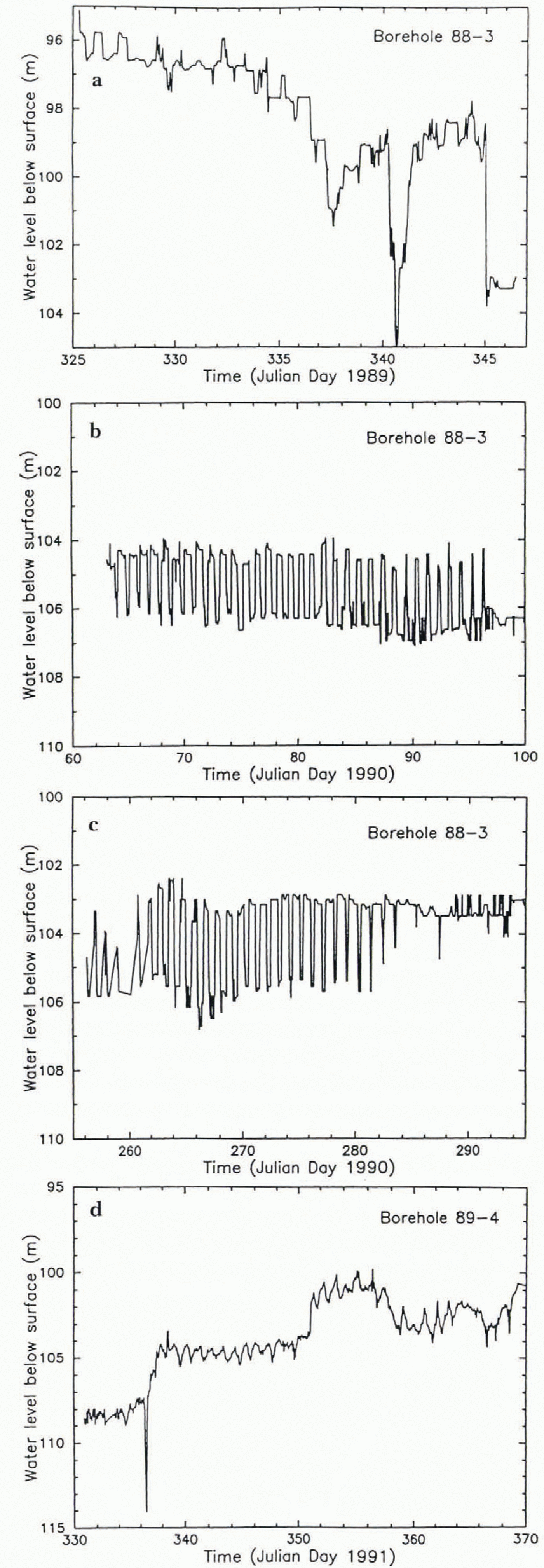
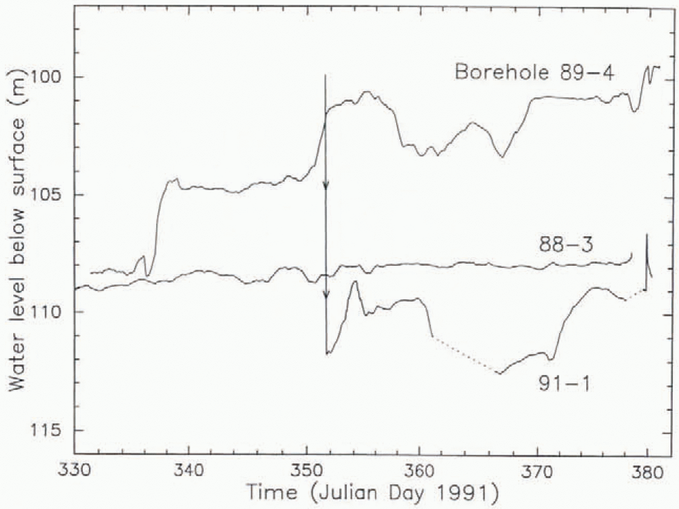
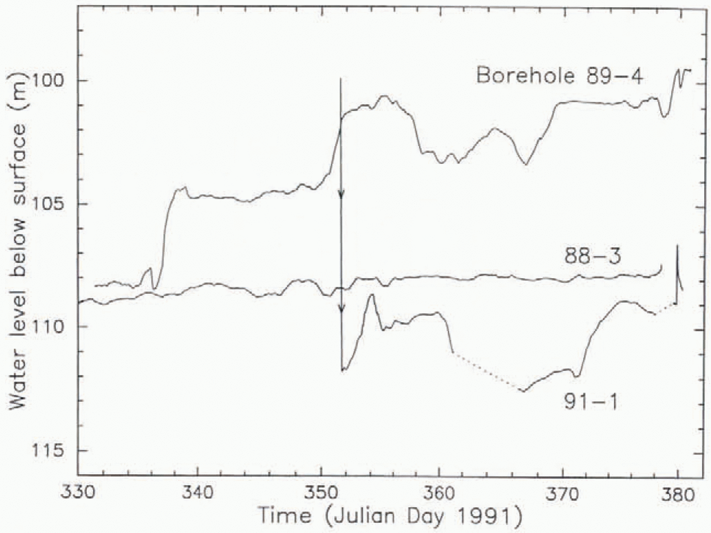
Of much interest is whether the pressures detected in different boreholes undergo correlated variations with time, as they should if connected to a basal water system at nearby points. The Opportunities to cheek on this, when two or more transducers were operating simultaneously, are provided by the data in Figures 10 and 13–15. Figure 10shows no correlation, but Figures 13–15 show strong to very strong correlations between pressure variations in 89–4 and 91–1. In Figure 10, the lack of correlation between the record from 88–3 and those from 89–1 and 91–1 may reflect the relatively large distance (500 m) between 83–3 and the other two holes (Fig. 4a). But the lack of correlation between the 89–4 and 91–1 records in Figure 10is troublesome, because these holes are only 25 m apart (Fig. 4a). (There may be a weak correlation between the 89–4 and 91–1 records if the latter is shifted forward by about 3 d, but we know of no reason for such a shift). The records from the same two boreholes in Figure 13. obtained 9 months later, are extremely close, reproducing even fine details such as the amplitudes and asymmetry of the individual diurnal peaks. And yet the records are not identical, either in the fine details or especially in the fact that the pressure values from 89–4 are systematically lower than those from 91–1 by about 10 m. This latter type of feature has been seen in other glaciers (Reference HodgeHodge, 1976, figs 8 and 9; Reference Kamb and EngelhardtKamb and Engelhardt, 1987. p.35. footnote) and therefore does not necessarily imply miscalibration of the pressure zero for one or both of the pressure transducers, such a large calibration error being unlikely.
Comparison of basal water-pressure records from boreholes 88–3,89–4 and 91–1 over the period 26 November 1991 to 15 January 1992. The original pressure records have been smoothed it with a 1 d running mean to damp short-period fluctuations, particularly diurnal ones. (The effect can be seen by comparing the 89–4 record here with the unsmoothed record in Figure 12d, which covers most of the same time period.) Arrowheads at the beginning of the 91–1 record are a reminder that the steep line represents the last part of the water-level drop at breakthrough (as in Fig. 9a). Data gaps are bridged with dotted lines. The peaks at the end of the 89–4 and 91–1 records are associated with the pressure-pulse propagation experiment discussed in section 8.
Diurnal fluctuation in basal watei pressure recorded from boreholes 89–4 and 91–1 over an 80 d period in 1992. (a) and (b) show the full period, while (c) and (d) show a 10 d period beginning on FD 260, to make visible the details of peak shape.

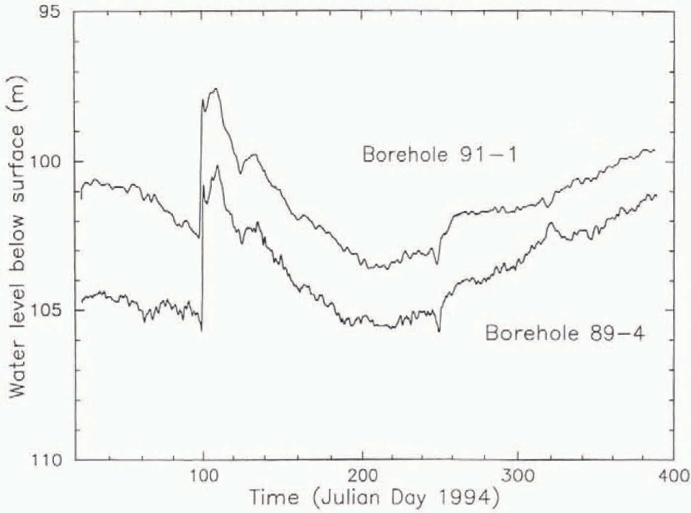
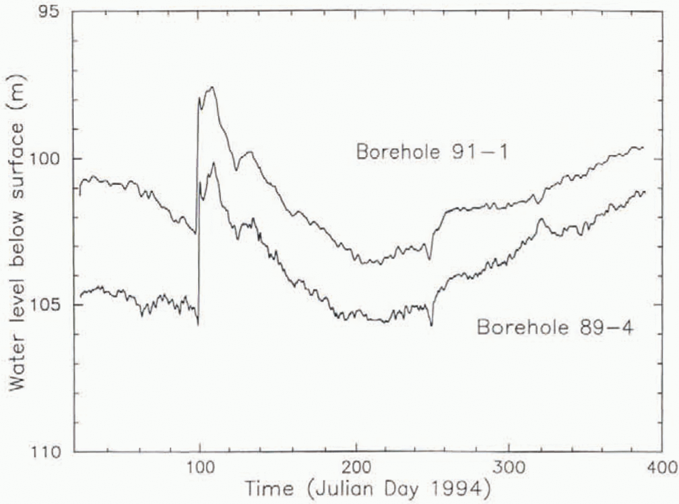
After a 1 year data gap in 1993, the pressure records in 1994 (Fig. 14) again show a strong correlation between bore holes 89–4 and 91–1. The correlation is not due to electrical cross-talk between the two transducers and their recording systems (data loggers), because from 1994 on they were electrically independent, including independent power supplies battery banks and solar panels). The offset between the reported pressure levels in the two holes, which had been ∼10m of water in 1992 (Fig. 13), had decreased to 4m by the beginning of 1994 and decreased gradually further to 1.5 m by the end of 1994 (Fig. 14) and to roughly 0 in 1995 (Fig. 15).
Comparison of basal water-pressure records from boreholes 89–4 and 91–1 during most of 1994.
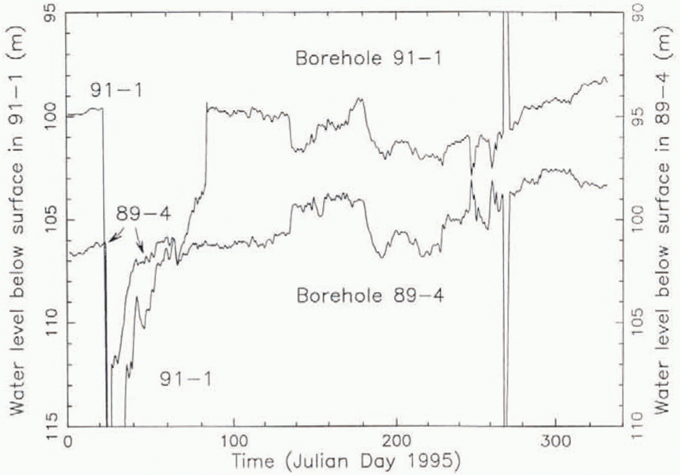
Comparison of basal water-pressure records from boreholes 89–4 and 91–1 during most of 1995. Note that for clarity the ordinate (water level) has been shifted by 5 m in the plot for 91–1 relative to the plot for 89–4, as indicated by the ordinate tabels on left and right. In the abrupt-drop event on FD 24, the curvefor 91–1 goes off scale down to 125 in. and 89–4 goes to 119 m. In the anti-correlatingspikes on JD 269. 91-1 goes off scale up to 74 m. and 89–4 goes down to 113 m.
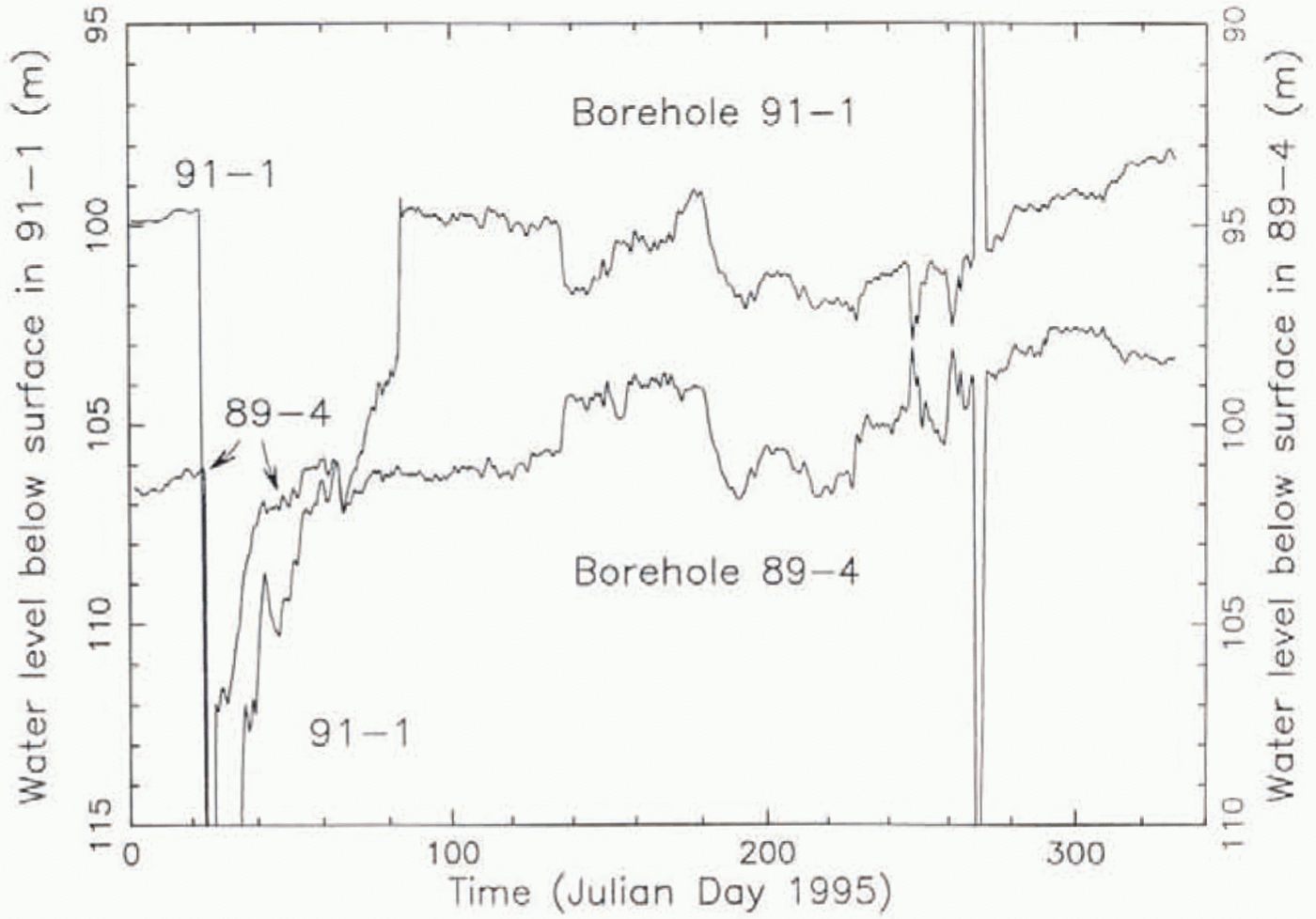
In 1995 a remarkable new feature became prominent in the pressure records from 89–4 and 91–1: the occurrence of anticorrelating peaks/troughs and rises/drops alongside many positively correlating events (Fig. 15). The first such anticorrelating event occurs in 1994 near JD 320 (Fig. 14). These events perhaps bear a relation lo the anticorrelations found by Reference Murray and ClarkeMurray and Clarke (1995)in borehole pressure records from Trapridge Glacier. The anticorrelatin was between boreholes connected and unconnected to the basal water system, whereas in our case both boreholes (89–4 and 91–1) had connected at least initially in a normal way. Reference Murray and ClarkeMurray and Clarke (1995)found one borehole that switched semi-diurnally between correlation and anticorrelation with the connected boreholes, which is at least slightly similar to the interspersal of correlating and anticorrelating events in Figure 15.
Although we do not have an explanation for the anticorrelating events interspersed with positively correlating events (Fig. 15), they provide an additional indication that the signal fluctuations are due to actual water-pressure variations rather than electrical noise generated in the two transducer/recorder systems.
We conclude that the two holes gave valid measurements of water pressure in the same basal system, at least some of the time. This supersedes the conclusion of a high noise level (short term 1 or 2 m of water, long term up to 5 m) reathed earlier in this section on the basis of Figure 7. It is possible dial at other times, such as the period of Figure 10. local hydraulic barriers intervened between 89–4 and 91–1 so that the two boreholes accessed difierent pressures in the basal water system, in the same way that the initial water levels at holes 88–1 and 88–2 differed by 9 m, or that the initial levels at 89–1, −2 and −3 differed by about 15 m from those at 89–, −5, and −6 (Fig. 4a; Table 1).
The following pressure events are of particular interest: (1) the large, abrupt basal water-pressure rise on JD 100 in 1994 (Fig. 14), followed by a slow recovery; (2) the very large, abrupt water-pressure drop on JD 24 in 1995 (Fig. 15), again followed by a slow recovery; and (3) the large anticorrelating spikes on 1995 JD 269 (Fig. 15). The asymmetric drop on JD 24 somewhat resembles such spikes in Figure 9a. In the JD 21 event the water levels reach the deepest levels ever recorded (119 and 125 m).
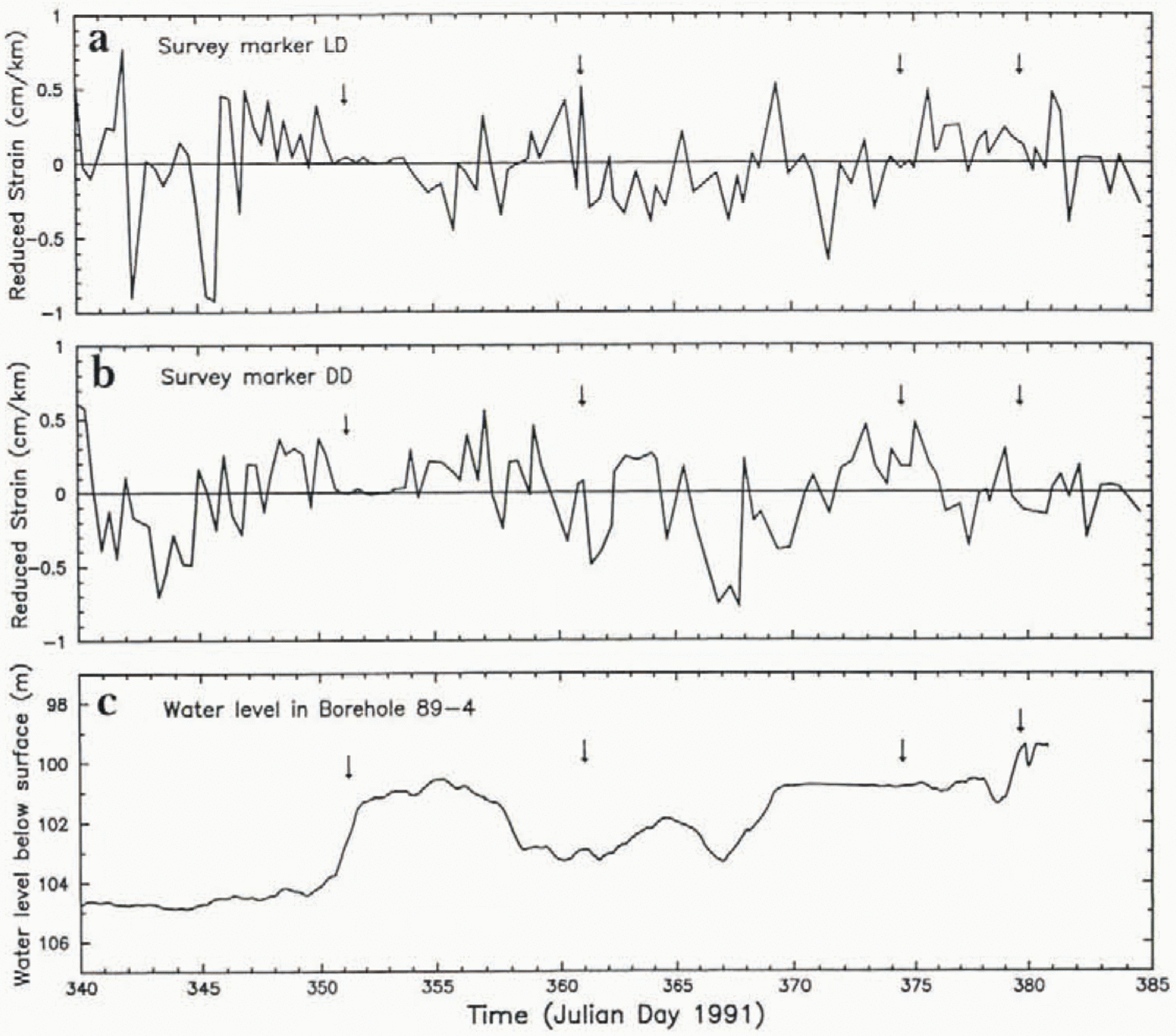
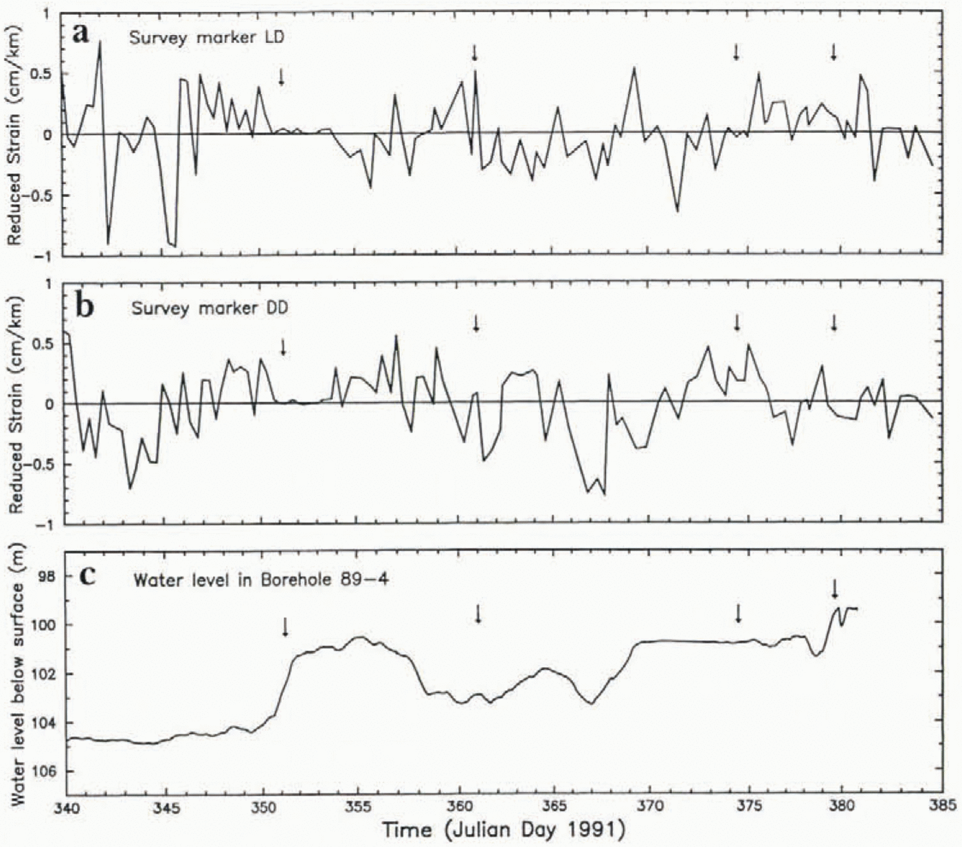
Also of much interest is whether there were variations of ice-stream motion that correlate with the observed variations of basal water pressure. At a point 7 km from UpB ’84, Reference Harrison, Echelmeyer and EngelhardtHarrison and others (1993, Fig. 2)measured the ice-stream motion relative to the slowly moving Unicorn (Fig. 1) over intervals of about 0.5 d during the period 1988 JD 334–362, which included the period during which the first pressure record from 88–3 was obtained (Fig. 9a). They found no significant variation in motion at the level of accuracy of 3.5% (3.5 mm d−1) whereas there were noteworthy variations in reponed pressure in 88–3. However, as discussed above, these variations to excessively high apparent pressures were not valid indications of pressure in the basal Water system. During the period 1991 JD 340–385 we operated in site area I a strain rosette with markers placed 2 km from a central electronic distance-measurement station in longitudinla and 45° diagonal directions, to look for changes in strain rate that might reflect changes in ice motion at UpB. Sample results are given in Figure 16. They show no indication of any significant changes in strain rate and no correlation between strain record and pressure record. There is also no correlation of pressure or velocity events with the times of borehole breakthrough and injection of water into the basal system (arrows in Fig. 16).
Comparison of surface longitudinal strain data with basal water-pressure data over the period 6 December 1991 to 19 January 1992. Surface strain is from two arms of a centered strain rosette: in (a), the strain is measured (by electronic distance meter) in the direction of flow, and in (b) it is measured in a direction 45° from the flow direction. “Redncedstrain” means that the strain due to a steady mean strain rate has been subtracted (e.g. 053 cm km−1d−1for (a)), so that any fluctuations in strain rate from the mean can more readily be detected. The pressure curve from hole 89–4 is the same as the 89–1 curve in Figure 10. The arrows indicate times of breakthrough (and resulting water injection into the basal water system) in the drilling of other boreholes.
The only instance of correlation between a change in ice-Stream motion and in basal water pressure in our observations to date is the following: in December 1995 a 26 d record of basal sliding and basal water pressure was obtained in borehole 95–2 (Fig. 2b), which showed a 4 d period of greatly reduced sliding rate that immediately followed a 2 d pulse of reduced water pressure.
6. Storage Capacity of Basal Water System and Boreholes
From the large and rapid drop in water level on borehole breakthrough (section 3) it is evident that the basal water system has a substantial capacity to store water injected into it in this way. A typical breakthrough from a starting water level of 20 m to a post-breakthrough water level of 105 m injects ∼12m3of water into the basal water system (see below). On several occasions we have tested the basal water system subsequent to breakthrough by pumping water into or out of a borehole, a standard method for evaluating the quality of the borehole’s hydraulic connection to the basal system (Reference EngelhardtEngelhardt, 1978, p.43; Reference IkenIken and Bindschadler, 1986, p. 104). In all cases there was little or no change in water level, generally less than a few meters, on pumping in or out.
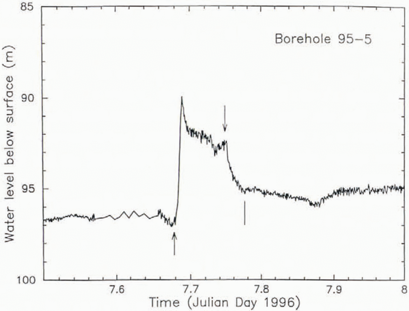
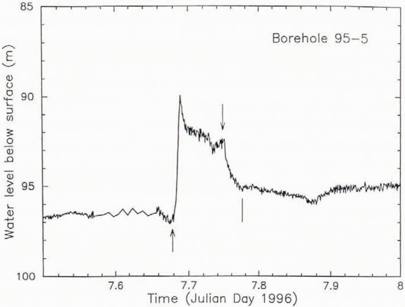
An example of pumping in is shown in Figure 17, from borehole 95–5. Pumping in caused an initial rapid rise in water level from 96.8 to 89.6m depth, after which the level subsided somewhat, so that by the end of 2 h pumping time the level was at 92.8m. At this point, pumping in was switched to pumping out, for 30 min, and the water level descended to 95.5 m, 1 m higher than at the start of the test. At a pumping-in rate of 60 1min−1, 7 m3of water was pumped into the basal system in this test, and 1.5 m 3was pumped out, at a rate of 49 1min−1. The behavior of the water level (Fig. 17) suggests that during pumping in, the hydraulic impedance of the connection to the basal system decreased somewhat.
Effect of pumping test on waterlevel in borehole 95–5, carried out on 7 January 1996, 1 d after breakthrough (shown in Fig. 3f). An upward-pointing arrow marks the start of pumping in, and a downward-pointing arow the start of pumpint out. Termination of pumping out is marked with a tick (without arrowhead). See text (section 6) for details
An example of pumping out is a test carried out in hole 91–1 on 19 December 1991. Water was pumped from the hole at a rate of 25 1min −1for 80 min, for a total of 2 m3, and the water level dropped from 110.6 to 110.8 m. Upon cessation of pumping the level went back up to 110.6 m.
Although in such tests, carried out after breakthrough, the basal water system yields water freely, with little or no indication of drawdown, there is a question whether the system would be able to deliver water if it were tested with-out the prior injection of the large volume of water that occurs in breakthrough. Two attempts to make such a test were undertaken. The first, in the drilling of hole 92–1, failed because the capacity of the well pump was insufficient to draw the water level down to below 90 m depth. The second, in the drilling of hole 95–3, failed because the hole bottomed in frozen till and did not connect to the basal water system, as shown by the fact that its water level was raised a few hours s later to 57 m by pumping in (sec section 3). There is a possibility that the lowering of the pre-breakthrougb water level to 107 m, a typical initial post-breakthrough level, somehow prevented a connection with the basal water system from being made, but this seems unlikely, because breakthrough has occurred with a difference of only 14 m between the pre- and post-breakthrough water levels (see Fig. 5a, at JD 355.4).
Pumping tests in blind holes, before breakthrough, provide information on the borehole diameter in the upper 100 m of the hole, which is needed for the interpretations in section 9. For example, on 1 December 1992 the water level in hole 92–1 during drilling was drawn down from 20 to 92 in depth by pumping water out of the hole at a net rate of 37 1min −1for 168 min. (The water-level lowering in this pump-down can be seen in Figure 5dnear JD 335.7.) This corresponds to an average borehole diameter of 23 cm for each of the two holes — main borehole and auxiliary water-well hole—that were drawn down in the test. Likewise, on 29 December 1995. hole 95–3 during drilling was pumped down from 32 to 72 m water-level depth at a rate of 49 1min−1for 175 min. The corresponding average diameter of the two holes (main and water-well) is 37 cm. These estimates are considerably larger than the nominal 10cm borehole diameter produced in the initial drilling; the enlargement is probably due to the extra heat introduced into the upper part of the hole to keep the water-well pump and its hose and electrical cable from freezing in. For the interpretations in section 9 we adopt here an average diameter of 30 cm for main hole and water-well hole in the upper 100 m. This figure is. however, rather uncertain, as indicated by the substantial discrepancy between the two estimates (23 and 37 cm). In section 9 We will use r s=  for the radius of the equivalent single hole with the same cross-sectional area in the nrar-surfacc 100 m of the hole.
7. Transport in the Basal Water System
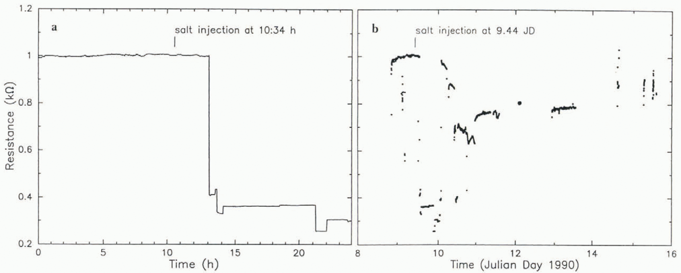
To provide information on the movement of water in the basal system a salt-tracer experiment was carried out as follows. A concentrated salt solution was released at the bottom of borehole 89–6, and the DC electrical resistance between electrodes at the bottom of holes 89–4 and 89–5, 65 m downstream from 89–6, was followed as a function of time. Release of the salt was followed by pumping water into the hole for several minutes to assure, in view of the results of pumping experiments (section 6), that the salt water would be injected into the basal system around the bottom of the hole. The distance between the electrodes (distance between holes 89–4 and 89–5) was 30 m. A sharp decrease in resistance between the electrodes was detected 2.4 h after the salt was released (Fig. 18a). This corresponds to an average propagation velocity of 7.5 mm s−1for the leading edge of the salt cloud.
Results of salt transport experiment carried out on 9 January 1990. (a) Electrical resistance (DC) between electrodes at the bottum of boreholes 89–4 and 89–5, as a function of time for 24 h centered on the injection time; salt solution was injected into the basal water system from borehole 89–6 at the time indicated by the tich mark. (b) Resistance between 80–4 and 80–5 vs time over a 7 d period including the sait injection.
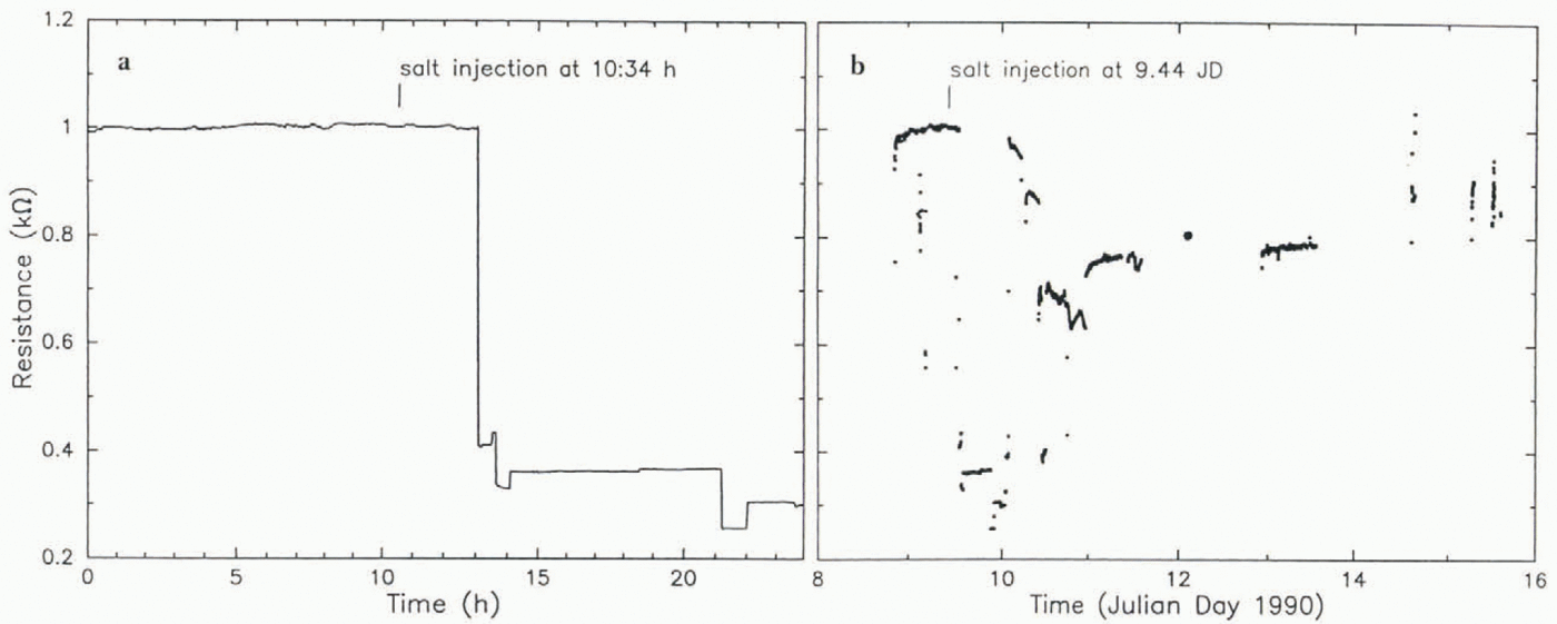
Although the above result seems straightforward, indications of greater complexity in the system are given by the complete data set for the inter-eleclrode resistance over the course of 7 d (Fig. 18b), which shows several other resistance jumps in addition to the one in Figure 18a.
8. Pressure-Pulse Propagation in the Basal Water System
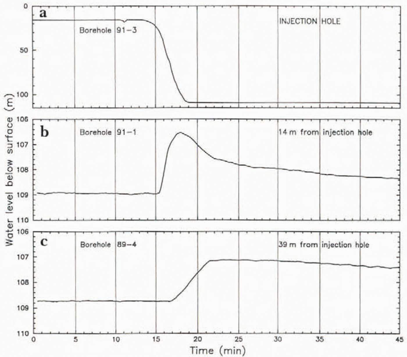
To reveal how the basal water system functions as water is injected into it during breakthrough, the basal water pressures in boreholes 89–4 and 91–1 were monitored closely as the drilling of hole 91–3 was completed and breakthrough occurred; the drop in water level in 91–3 was recorded also. Hole 91–1 was 14 m distant from hole 91–3. and hole 89–4 was 39m distant from 91–3 (see Fig. 2a). The results — basal water pressure vs time in the three holes — are plotted in Figure 19. They show a fairly normal breakthrough-pressure drop at the injection hole (91–3), followed by the arrival of a pressure pulse at 14 and then at 39 m from the injection hole. The onset of the injection-pressure drop at 91–3 is at about 14 min on the time-scale of Figure 19, while the onset of the pressure rise 14 m away is at about 15.5 min, and 39m away at about 17 min on the same scale. We assume that the ouset of the pressure drop at 91–3 marks the time when a sudden, step-like rise in pressure was introduced into the basal water system there; hence, the propagation time of the pressure-rise onset was 1.5 min to the 14 m distant point and 3 min to the 39 m distant point, a propagation speed of about 11m min−1. The pressure pulse that arriv ed at 14 m is an asymmetric peak (rapid rise, slow decay), while by the time the pulse reached 39 m it had become a ramp with relatively slow rise and even much slower decay (Fig, 19b and c). If for the time of peak pressure at the injection point we take the onset and at 39 m we take the sharp bend at the top of the ramp, then the propagation time for the pressure peak is 4 min from injection to 14 m, and 7.5 min from injection to 39 m, at a speed of about 5 m min−1. The peak injection pressure, corresponding to a water level about 90 m above the post-injection level at the injection point, is greatly attenuated lo about 2.5m above the pre-injection level at 14 m, and further to 1.5 m above the pre-injection level at 39 m.
Results of pressure-pulse propagation experiment in the basal waler system, carried out on 14 January 1992. (a) Water level in borehole 91–3 vs time during drilling and as breakthrough occurs starting at 14 min on the plotted time-scale with arbitry zero; this is the injection hole, from which water is forcefully injected into the basal water system during breakthrough. (b) Basal water pressure (expressed as water level) vs time in borehole 91–1. 14 m from the injection hole, (c) Basal water pressure vs time in borehole 89–4. 39 m from the injection hole.
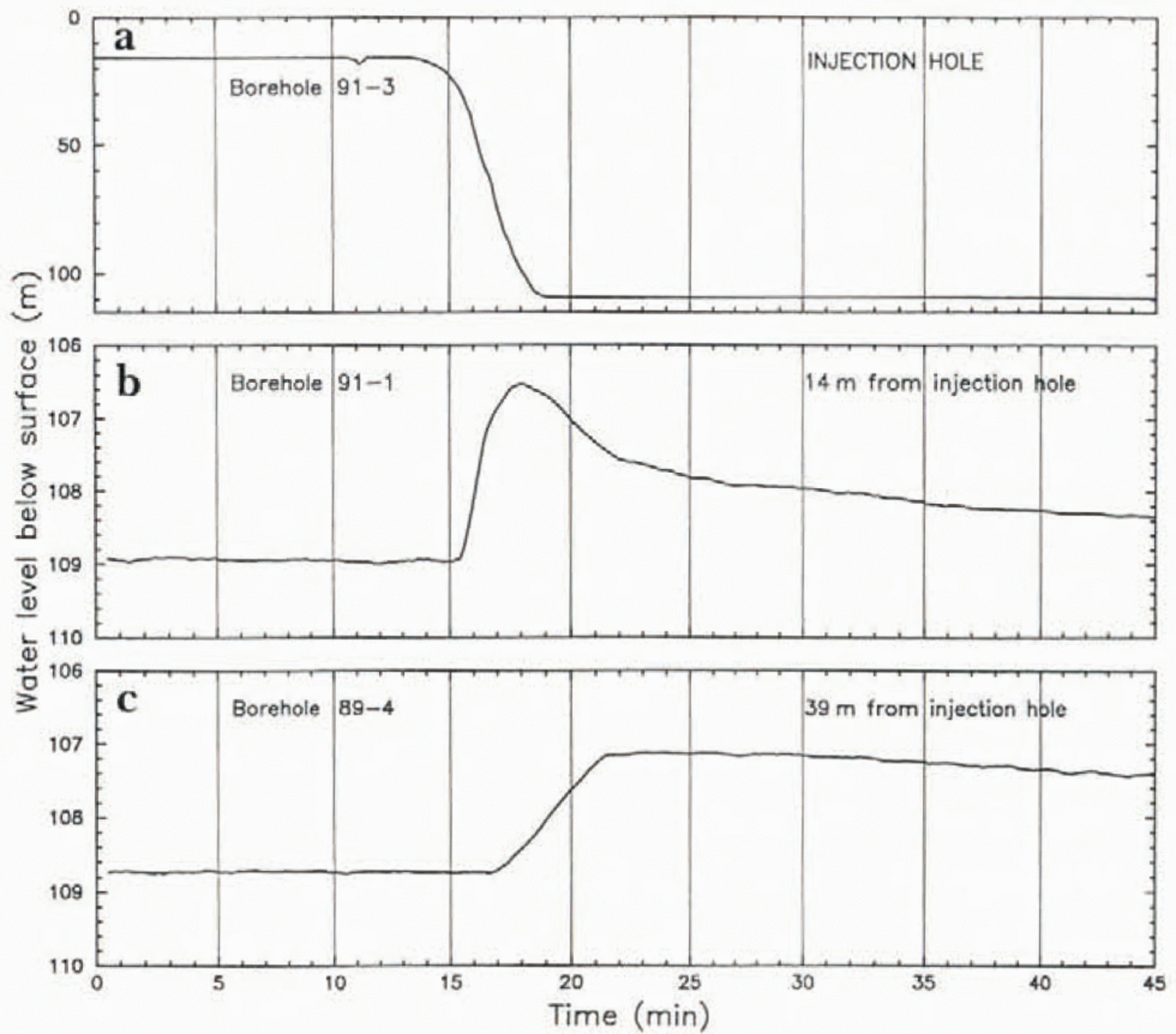
The propagation speed (∼0.6 km h−1for onset, ∼0.3 km h −1for peak) and the change in pulse shape with propagation rather resemble the speed and changing shape of pressure pulses in propagating mini-surges in Variegated Glacier, Alaska (Reference Kamb and EngelhardtKamb and Engelhardt, 1987, table III and figs 8b and f, 10b and f), although the horizontal scales of attenuation are very different, ∼25 m vs 1.7 km.
These results provide a strong constraint on the nature of the basal water system, as explained in section 9b and c.
9. Interpretation: Nature of the Basal Water System
The existence of a basal water system capable of accepting water in volumes of ≳10 m3and returning it in comparable quantity is proved by the behavior of borehole water levels in breakthrough (section 3) and in subsequent pumping tesis (section 6). Because boreholes almost always have immediate local access to this system (22 out of 24 holes had immediate access and another gained access in 9h), it must be a widely dispersed conduit system quite different from a classical R-tunnels system consisting of one or a few R-tunnels widely spaced across the 35 km width of Ice Stream B2. This conclusion is reinforced by the application of R-tunnel theory to Ice Stream B by Reference BindschadlerBindschadler (1983, p. 11), which gives an effective basal pressure of about 4 bar in the vicinity of UpB, considerably larger than the observed values in the range 0–1.7 bar ( Table 1; section 3).
A basal-till aquifer would be a suitably dispersed basal system, but in order to transport the water produced by basal melting (distributed source) the till would need to have a hydraulic conductivity in the range 0.02–0.06 m s −1(Reference Lingle, Brown, Van der Veen and OerlemansLingle and Brown, 1987, p. 274), vastly greater than the measured value ∼10 ms−9(Reference Engelhardt, Humphrey, Kamb and FahnestockEngelhardt and others, 1990, p.248). Groundwater flow modeling by S. Tulaczyk (personal communication, 1996) shows that the required conductivity would be reduced only a small amount by including the bedrock beneath the till in the aquifer model, if the hydraulic conductivities of bedrock and till are comparable, as follows from their lithologic similarity (unpublished information from S. Tulaczyk and others).
The modeling by Reference Stone and ClarkeStone and Clarke (1993, Fig. 4 and Table 1)of the water-level drop in a borehole that bottoms in an aquifer 0.04 m thick, with hydraulic conductivity 0.067 m s , and drop time about 20 s, can be used to set a lower limit on the hydraulic conductivity of a 10m thick till aquifer that would be required in order to give the drop times of 1–3 min that we observe. Assuming that the drop time is inversely proportional to the hydraulic conductivity and the aquifer thickness, and directly proportional to r s2as in Equation 9below, we obtain on this basis an estimated minimum hydraulic conductivity of (0.5–1.4) × 10−3ms−1. It is a minimum estimate because the model assumes that the borehole penetrates through the aquifer (Reference Stone and ClarkeStone and Clarke, 1993, Fig. 1) whereas our boreholes reach only the top of the till. The estimate is much higher than the measured hydraulic conductivity of the till as noted above (∼10−9m s−1). The foregoing considerations rule out a till aquifer as the basal water system of Ice Stream B.
9a. Gap-conduit model
Among the various types of basal water system models that have been considered (Reference Kamb, Stone and RuncornKamb, 1993, p. 29–30, 52–59, 61, 68, 72–74), the most promising at first sight is a version of the “water film” model originally due to Reference WeertmanWeertman (1972), in which there is a narrow gap, of width δ, between the ice sole and the underlying bed. It is here called the gap-conduit model. If the flow in the gap is laminar, as assumed by Weertman, the average water-flow velocity u w(averaged over the width δ) is given by the Poiseuille equation

where Γ is the hydraulic grathent

Zwbeing the elevation of the phreatic surface, that is, the water level in a real or imaginary manometer tube (such as a borehole connected to the basal water system at a given point and reporting the basal water pressure PBwat that point. ZBis the elevation of the bed, ∇2the two-dimensional gradient operator  (where zis vertical and
 and
 are unit vectors along the xand yaxes), η wthe viscosity of water, ρwthe density of water, gthe gravitational acceleration, and ϕan areal fraction to be discussed later (for now, ϕ = 1). This model can be applied to the borehole breakthrough phenomenon as follows. Assume cylindrical symmetry, so that the variables depend only on radial distance rfrom the borehole, and
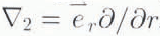 . Assume a level bed with a constant gap thickness δ, and write the continuity condition for water flowing radially outward from the borehole:

The water flux Qwis independent of radial coordinate r > robecause the entire Water source is at ro, the radius of the borehole. Using Equations (1) and (2) we have

Kis defined in Equation 1. Integrating from rooutward,

where Zois the water level in the borehole. For definiteness we take the datum for Zwto be the undisturbed pre-break-through water level. Suppose that at some large distance Lfrom the borehole the water level remains at the undisturbed value zw= 0. Then Equation 5becomes

Which serves to determine Qw. Now Qwis the rate at which water is leaving the borehole, so the drop in borehole water level zo(t)as a function of time tis given by

where rsis the near-surface equivalent borehole radius, explained in section 6. Equation 7can be integrated (assuming Lfixed) to give the exponential

where zo(0) is the borehole water level (relative to the undisturbed level) at time of breakthrough (t= 0) and the time constant Tis

Evaluation of Tfor each of the water-level drop curves in Figure 3gives a value of the gap width δ from Equation 9, based on parameters η w= 0.0018 Pa s, ro= 5 cm, rs= 21 cm (section 6), and L= 1 km. Tis evaluated from the maximum drop rate (–dz o/dt)max; from Equation 8,

Here zo(0) is the initial extra water column, equal to minus the difference between the pre-breakthrough and post-breakthrough water-level depths (for which values are listed in Table 1). For the curves in Figure 3that depart from strict exponential form, the evaluation of Tfrom Equation 10is somewhat arbitrary. Also arbitrary is the choice of L, but the result is insensitive to L: variation of Lfrom 100m to 10 km causes only a 16% variation in δ.
The gap widths δ calculated from the above model ( Table 1) are clustered in the range 1.4–2.0 mm.
The same model was applied by Reference Stone and ClarkeWeertman (1970)to the rise of water that occurred upon reaching bottom in the 2164 m deep Byrd borehole. The water rose 42 m in 10h, which leads to δ = 0.14 mm. Weertman noted that this is a minimum estimate of the gap thickness before disturbance by the borehole, because for water flow radially inward to the borehole the water pressure near the hole is reduced, which will allow the ice to sag and the gap to narrow.
On the other hand, in the breakthroughs that we have experienced, the water flow is always outward from the hole and the water pressure in the gap is increased, which can raise the ice and enlarge the gap. Thus, the values of δ that we calculate in Table 1are maximum model estimates of the original gap width.
Another difference between the Byrd situation and ours is that our water-flow velocities during breakthrough are much faster, corresponding to the much shorter drop times (2–3 min vs 10h). At the high velocities near the borehole, the flow outward in the gap would be turbulent, rather than laminar assumed in the model. From our values dz o/dt= –35 m min–1and rs= 0.21 m one can calculate that the Reynolds number in the gap would be ∼105near the borehole wall and would decrease outward as 1/r, reaching a value ∼2000 at r≈ 3 m the flow would be laminar. In the laminar-flow model, as expressed in Equation 5, only 35%,, of the total drop in hydraulic head in the gap occurs over the interval from r= 0.05 m to r= 3 m. Thus, changing the model to one with turbulent flow replacing Equation 1over this interval would probably not have a great effect on the results. Analytical formulation of the transition from turbulent to laminar flow in the gap, as the flow is followed radially outward from a borehole, is discussed by Reference Stone and ClarkeStone and Clarke (1993, p.338). In the limiting case of turbulent flow according to the Manning equation in place of Equation 1at all distances r, one finds that for the same value of dz o/dt, driven by a hydraulic head of 70 m, with L= 1 km. the required gap width is δ = 15 mm for a Manning roughness M= 0.1 m–1/3s (as commonly assumed), or δ = 4 mm for M= 0.01 m–1/3s. Thus the effect of turbulent flow in the model will be to increase the required gap width δ but it does not change the basic picture.
A modification of the gap-conduit model is called for whenever the basal water pressure is less than the ice over-burden pressure, as we generally observe and as must generally be the case in the natural state undisturbed by a borehole. In this case a gap conduit cannot intervene continuously between the bed and the ice sole, because the ice would not be fully supported by the water pressure in the gap below. The gap can be present only over a fraction of the area of the bed: the areas where the gap is not present and where the sole is in direct Contact with the bed must bear a enough vertical stress that, in combination with the water pressure in the gap, the ice overburden pressure is on average supported. If the areal fraction of the bed occupied by the gap, here designated ϕ, is distributed over the bed in such a way that all of it is able lo transmit water flow (as in a braided stream network, for example), then the average water flux can be expressed by introducing ϕ as a factor in Equation 1. (The flux of water per unit width is u wδwhen now u wis averaged both vertically and horizontally, uwbeing 0 outside the gap). Allev (1989a, p. 14; 1989b, p. 119) and Reference KambKamb (1991, p. 16,590)used “incomplete-gap conduit” models of this type (see Reference Kamb, Stone and RuncornKamb, 1993, p. 56, 72; it is called the “punctured water sheet” model by Reference WeertmanWeertman, (1970, p. 312)). This modification from the “complete-gap conduit” model does not have a strong effect on the gap thickness δ needed in the model. For example, if ϕ = 0.5, the δ values in Table 1are increased by 25%.
The incomplete-gap conduit model can also be applied to the results of the salt-tracer experiment (section 7). If we assume that the leading edge of the salt cloud is transported at the mean velocity u wgiven by Equation 1with the hydraulic grathent Γ set equal to the regional surface slope α= 0.1°, then the measured transport rate u w= 7 mm s−1corresponds via Equalion (1) (with ϕ = 0.5) to a gap thickness δ = 4.3 mm. This is not greatly different from the δ = 2.0 mm given by the breakthrough interpretation above, with allowance for ϕ = 0.5. Uncertainty is introduced into this comparison by the effects of turbulent flow and by the assumption of flow under the regional grathent α rather than under a local grathent that might be considerably different. In principle the local grathent should be obtainable from the measured water levels (Fig. 4a) at the three boreholes involved in the salt experiment (section 7), but that cannot be done reliably at the ±1 m uncertainty level of the values. The arbitrary assignment ϕ = 0.5 is another, but minor, source of uncertainty. There is in addition a ∼20% uncertainty in the δ = 2.0 mm figure due to the uncertainty of rsin Equation 9(section 6).
Λ further check on the gap-conduit model of transport in the basal water system is provided by comparing the water flux q w= u wδ= 0.3cm2s–1in this model with flux values from theoretical model calculations of basal melting upstream from UpB. From frictionla heating in a soft-bed model of the ice stream, Reference Alley, Blankenship, Rooney and BentleyAlley and others (1989, Fig. 2)obtain qw—0.8 cm2s −1at UpB. From a quite different thermo-mechanical model, Reference Lingle, Brown, Van der Veen and OerlemansLingle and Brown (1987, Fig. 9)estimated qwin the range 1.5–5.5 cm2s−1. Reference Weertman and BirchfieldWeertman and Birchfield (1982, p.317)took qwimplicitly to be 4cm2s−1in their gap-conduit model of the West Antarctic ice streams, in which they used δ = 8 mm and u w= 5 cm s−1. Reference Alley, Blankenship, Rooney and BentleyAlley and others’ (1989)theoretical model involves an incomplete-gap conduit with δ = 5 mm and u w= 1.6 cm s−1. (Values for ϕ are not given.) The agreement of the above theoretical values with our observed quantity u w= 0.7 cm s−1, or with our derived quantity qw= 0.3 cm2s −1obtained from u wvia the gap-conduit model, is rough at best, but adequate to generate hope that the gap-conduit model is on the right track.
9b. Pressure-pulse propagation
If prior to breakthrough there exists at the base of the ice a gap-conduit system with gap thickness δ ∼ 1 mm, then when a pressure source with large hydraulic compliance is suddenly connected to this system, as happens when breakthrough occurs in a borehole, the applied pressure should propagate outward from the borehole through the conduit system at the speed of sound in water, 1400 m s−1. The observations discussed in section 8 and show n in Figure 19demonstrate that the pressure-wave propagation is very much slower, about 0.2 m s−1. This slowness is not attributable to substantial hydraulic compliance of the pressure-transducer installations in 89-4 and 91-1, for two reasons: (1) These holes had ample time to freeze up, ai least in their upper part (16 d for 91-1, 2 years for 89-4), and the holes therefore did not provide a compliance-giving connection between the transducer at the bottom and a free surface against the atmosphere above, as freshly drilled holes do. (2) Such compliance would slow the rise of pressure at the transducer but would not retard its onset, whereas a substantial retardation of the ouset clearly occurred (1.5 min in 89–4, 3 min in 91–1) (see Fig. 19).
The assertion that the pressure pulse will propagate with the speed of sound is subject to the proviso that the propagation speed is not significantly affected by the viscosity of water. The effect of viscosity can be estimated by formulating the equation for pressure propagation in the gap in the presence of viscous drag from the walls. The formulation is simplified to one-dimensional by averaging over the gap width and writing the equation in terms of the mean velocity u w, or, rather, in terms of the mean displacement Uin the propagation direction xwhere ∂U/∂t= u w:

Here kis the bulk modulus of water. The inertial term, on the left, and the pressure-grathent term (first term) on the right, which is expressed in terms of the xgrathent of the dilatation for one-dimensional displacement U, are the normal terms in the sound-propagation equation; with η wset to zero they give propagation of pressure waves with a speed  . Viscous drag enters via the last term in Equalion (11), which is 2τ/δ, where τis the shear stress on one wall of the gap. (On the other wall the shear stress is equal and opposite; both walls contribute equally to the drag.) τis η wtimes the shear strain rate at the wall, which is calculated from a parabolic velocity profile across the gap, parameterized in terms of u w(= ∂U/∂t), with velocity uw= 0 at the walls. This calculation has the same basis as the one that gives the Poiseuille Equation 1, except that in Equation 11we set ϕ = 1. The δ in 2τ/δcomes from averaging over the gap width.
The result in Equation 11can be written in a form more suitable for our use by differentiating with respect to xand substituting P= –k∂U/∂t, where P(x,t)is the water pressure:

where a= 6η w/ ρ wδ 2.
Equation 12has the form of the telegraph equation, whose solution (Reference Bronstein and SemendjajewBrcmstein and Semendjajew, 1987, p. 490) for initial conditions P(x,0) = P0(x)and 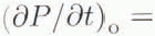 Pt(x) at t= 0 is

where

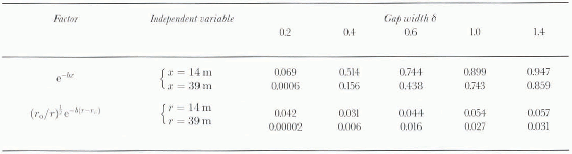
and where I0and I1are the modified Bessel functions of the first kind, of order 0 and 1. The part of the solution enclosed in curly brackets, with its arguments (x — ct)and (x + ct), represents waves travelling forward and backward with the normal sound speed c. Thus the pulse propagation speed is not affected by viscosity. The pulse amplitude is. however, attenuated by the exponential factor exp (-at)in Equation 13, which, for a pulse propagating with speed c, can be expressed in terms of propagation distance xas an attenuation factor exp (−bx)where

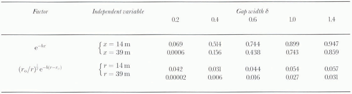
Thus the attenuation is an increasing function of viscosity η wand a strongly decreasing function of gap width via the factor l/δ2in Equation 15. For propagation distances involved here, x= 14 or 39 m, there is a rather rapid change from small to large attenuation over the range of gap values δ =1–0.2 mm. This is shown by the attenuation factor values exp (−bx)in Table 2. Also given in Table 2are attenuation factors (r o/r)1/2exp [−b(r − r0)]that incorporate the 1/r 1/2dependence expected from geometrical spreading in the absence of viscous attenuation (b= 0) for a cylindrical sound wave emanating from a cylindrical source of radius r = ro= 0.05 m. For a gap δ = 1.4 mm, as calculated from the gap-conduit model for borehole 91–3 ( Table 1), an initial water column of 93 m (above the equilibrium water level) at breakthrough should be attenuated to a height of 5.3 m at a distance of 14 m from the injection hole, and to 2.9 m at 39 m distance. An abrupt rise in basal water pressure to these levels should occur essentially immediately at breakthrough, without retardation (or, more precisely, with the retardation of the sound wave, 0.01 or 0.03 s). Thus the effect of viscosity on sound-wave propagation cannot explain the observation that the onset of the pressure pulse arriving at 14 and 39 in is retarded by 1.5 and 3min from the breakthrough time, and that the onset is an emergent ramp rather than an abrupt step-up in pressure. The observed pressure-pulse heights (2.5 and 1.5 m) are of the order expected for the sound wave (5.3 and 2.9 m), but the are retarded by 4 and 7.5 min relative to the expected sound-wave arrival.
Sound-wave attenuation factors exp(−bx) and (r o/r)1/2exp [−b(r − ro)]as a function of gap width δ (mm) and propagation distance x or radial distance r (with ro= 0.05 m)
The observed pressure-pulse heights at 14 and 39 m are much smaller than expected on the basis of the gap-conduit model with δ≅ 1.7 mm: according to Equations (5) and (6), combined so as to eliminate Qw, the equivalent water level zw(relative to the datum at r = L)should vary with ras

For an initial water column z0= 93 in, for ro= 5 cm, and L= 1km. Equation 16 gives = 34.5m at r= 14 m, and Zw= 26 m at r= 39 m, The observed peak heights are zw= 2.5 and 1.5 m, an order of magnitude smaller than expected values.
The several foregoing contradictions between borehole observations and model expectations based on the gap-conduit model adjusted to account for the water-level drop curves on breakthrough (requiring δ≅ 1.7 mm), as discussed above, put the gap-conduit model into serious doubt and call for an alternative model of the breakthrough phenomenon.
9c. Gap-opening model
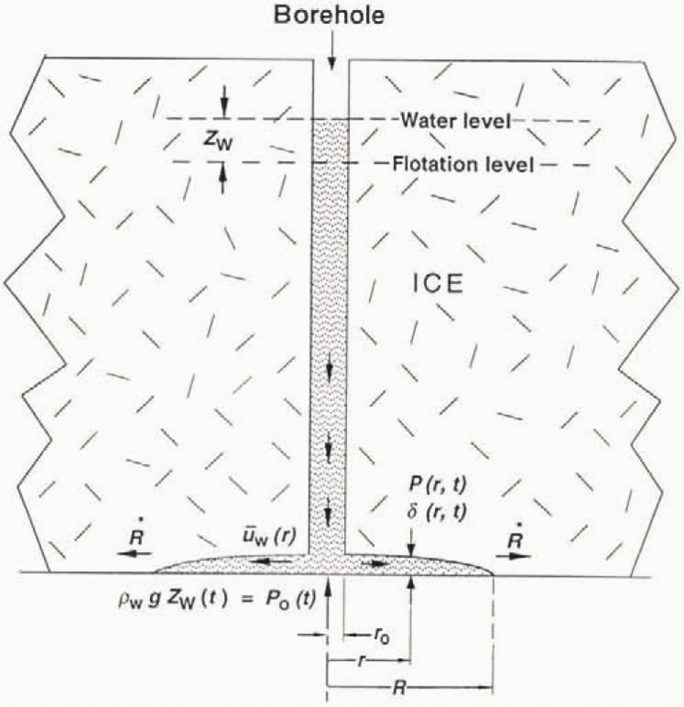
The above considerations lead to the idea that initially, prior to breakthrough, there is not a gap of millimeter thickness between ice sole and bed. Instead, such a gap forms and opens up during the breakthrough and water-level-drop event, by a slight local uplift of the ice mass around the borehole. The uplift is caused by the lifting action of the water injected along the bed at pressures above flotation. The opening of the gap proceeds in the manner sketched in Figure 20. The water intrudes along the ice/bed interface to form a thin, lens-shaped layer with feather-edge at radius R(t)expanding outward with velocity  The gap width δ(r, t)is now a function of radial coordinate and time, generally decreasing with rand increasing with t. Water at the bottom of the borehole, under pressure Ρo(t) due to the column of water above, enters the gap at r = roand flows radially outward at velocity u w(r, t), driven by the radial gradient of the water pressure P(r, t)in the gap. The ice above the gap is lifted up due to the distribution of pressure P(r, t)acting on its base, with an uplift rate
 that depends on the ice viscosity. In this way the gap is opened up and water from the borehole becomes stored there.
Diagram of the gap-opening model of water injection into the basal water system on breakthrough. Water in the borehole and in the injected lens-shaped layer of water at the base of the ice is shown shaded, r is radial distance from the botehole axis, rois the borehole radius, and t is time Δ(r,t) is the local gap width, P(r,t) the local uplift pressure of water (water pressure minus ice overburden pressure), and Po(t) the uplift pressure of water (water pressure minus ice overburden pressure), and Po(t) the uplife pressure at the bottom of the borehole, directly related to the height of ht borehole water level above the flotation level, as indicted. u w(r, t) is the local flow velocity of water radially outward, averaged over the gap width. R(t) is the (imagined) radius of the water lens (see text), and R its rate of advance.
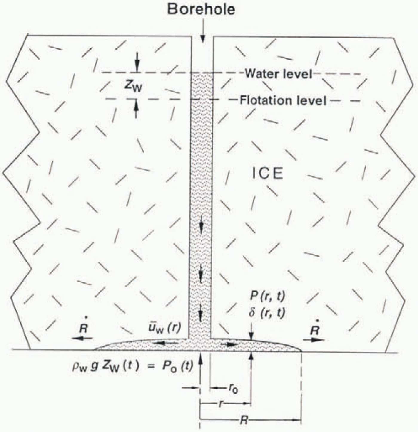
The validity of the geometry of this model can be roughly assessed by calculating the gap thickness at the borehole, δo,needed to store the water volume injected into the gap. For hole 91–3 we can make the calculation twice: at the onset of pressure rise in 91–1, when the radius of the lens-shaped, laccolith-like body of intruded water just reaches R= 11 m (the distance from 91–1 to 91–3), and at the onset in 89–4, when the radius just reaches R= 39 m. The volume of water stored at each of these times is calculated from the effective borehole radius rs= 21 em (section 6) and the drop in water level at these times, which is 10 and 54 m (see Fig. 19a). Assume that the lens shape is parabolic, δ(r) = δ o[1 – (r 2/R 2)]. Then on the above basis we calculate δo= 4.5 mm at R= 14 m. and δo= 3 mm at R= 39 m. We expect δo, to increase with time and thus with R(because the-gap should open progressively during the time that water pressure in excess of overburden is applied), so the inverted sequence for these values of δoindicates error, but the estimated order of magnitude of δo,a few millimeters, seems reasonable.
A quantitative evaluation of this gap-opening model is needed to assess its performance in relation to the observations discussed above. A quantitative formulation has the following five elements:
(1) Uplift of ice (of assumed linear rheology with viscosity η I) produced by water-pressure distribution P(r,t):
(17)
where
(18)K(k)being the Complete Elliptic Integral of the first kind (not related to the Kin Equation 1). Equations (17) and (18) are based on the displacement solution for a force acting normal to the surface of an elastic half-space (Reference Timoshenko and GoodierTimoshenko and (Goodier, 1951, p.365). The uplift pressure Pis the water pressure Pwless the constant ice overburden pressure PI.
(2) Water flow into storage in the widening gap:
(19)(3) Water-pressure distribution that drives the radial water flux qwby Poiseuille flow in the gap:
(20)The uplift pressure Po(t) = P(ro, t)is the water pressure at the bottom of the borehole minus the ice overburden pressure P1. It is equal to ρ wgz wwhere zwis the elevation of the water surface relative to the flotation level as datum (see Fig. 20).
(4) Enlargement of the gap:
(21)(5) Fall of the borehole water column:
(22)


A detailed derivation of Equations (17)–(22) will be given in a separate paper devoted to a comprehensive study of the gap-opening model. Here we pursue the behavior of the system only far enough to get an indication of whether ii is compatible with the observations.
Equations (17)–(20) describe the model system at any instant of time t = t1; given the gap-width distribution δ(r, t1)at that instant, they in principle permit the pressure distribution P(r, t1)and water flow qw(r. t1)to be determined, as well as the rate at which the gap is widening at each point,  . The development of the system with time is obtained from Equations (21) and (22) by introducing
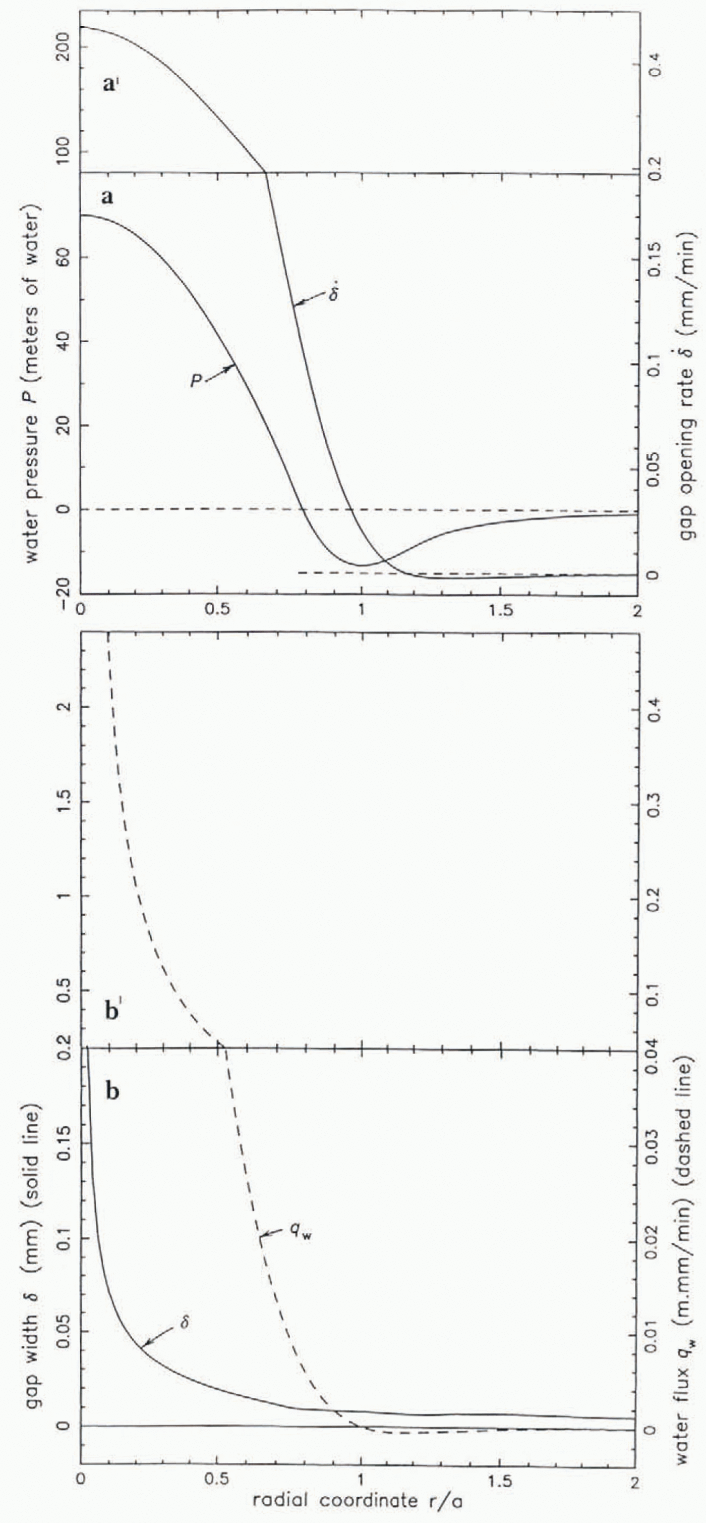
 and qw(r,t)from Equations (17) and (19). Solutions of Equations (17)–(20) have the character illustrated by Figure 21, which shows
 and qw(r)for the given gap-width distribution δ(r).Particularly noteworthy is the zone of negative pressure negative relative to the overburden pressure) outside the central zone that is pressurized by the inflowing water (qw> 0) from the borehole at r = ro. (In the plots in Figure 21the radial coordinate ris normalized by the radius aof the pressure minimum, taken to be a= 1 m; this ais unrelated to the ain Equations (12)–(14).) Also noteworthy is the fact that the gap width does not go completely to zero anywhere, so that the depiction in Figure 20, with δ going to zero at r = R, is not strictly valid; thus Rmust be defined in some other way, such as the radius at which ∂P/∂r= 0, as used below. The gap is, however, very narrow. ∼10 μm for r ≳ a in the solution in Figure 21.
Calculaled results of the gap-opening model, representing a solution of Equation (17)–(20). (а) Water-pressure distribution P(r) and corresponding gap-opening rate  . (b) Water flux q w(r) = u wδgap width δ(r). Radial coordinatr r/a is scated by the radius r = a at which P(r) has its minimum. Parameter values used n calculation are given in the text. Parameter values used in calculatio are given in the text. Note change of ordinate scales between panels a and a′, and between panels b and b ′.

As discussed in section 9a. the assumption of laminar flow in the gap, which is expressed in Equation 20, can break down near the borehole, where the flow is turbulent. The region of turbulent flow is, however, more restricted in the gap-opening model than in the gap-conduit model, because the storage of basal water in the opening gap reduces the water-flow velocity outward. For this reason, and in view of the moderate effects of turbulent flow assessed in section 9a, we expect that the gap-opening model would similarly be only moderately affected. In the model result shown in Figure 21the Reynolds number is less then 4 for r > 0.1 m, so there is no turbulent flow there, but this is for a different reason: the model represents the flow at an early stage of breakthrough, when the edge of the water lens has advanced only 1 m from the borehole (a= 1 m) and when all water-flow velocities are still small.
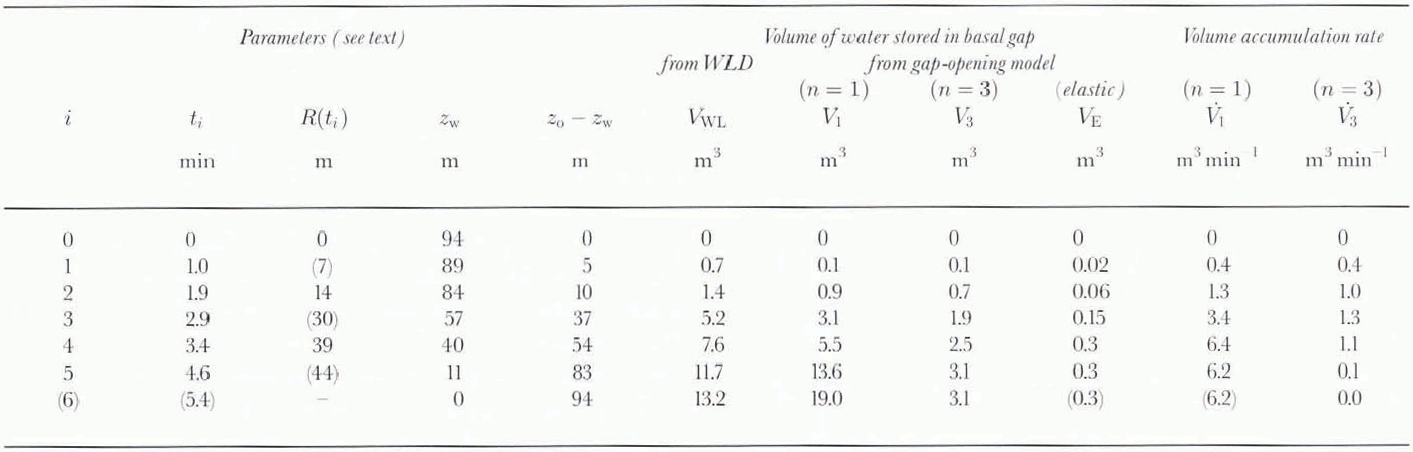
In this paper we cannot pursue the time dependence of solutions of Equations (17)–(22) except to the following limited extent. We consider the question whether the gap-opening model can account for the volume of water injected into the gap as a function of time in breakthrough events. The volume injected is an observational quantity VwL(t), calculated from the water-level drop Zw(t)as in section 6:

where, as before. zwis the height of the borehole water level above the equilibrium level, and Zois the initial level just before breakthrough. The model gives stored water volume Vi(t)from Equation 22, which can be rewritten, following Equation 23with z w(r o, t) = P(r o, t)/ρ wgand z o= P o/ρ wg:

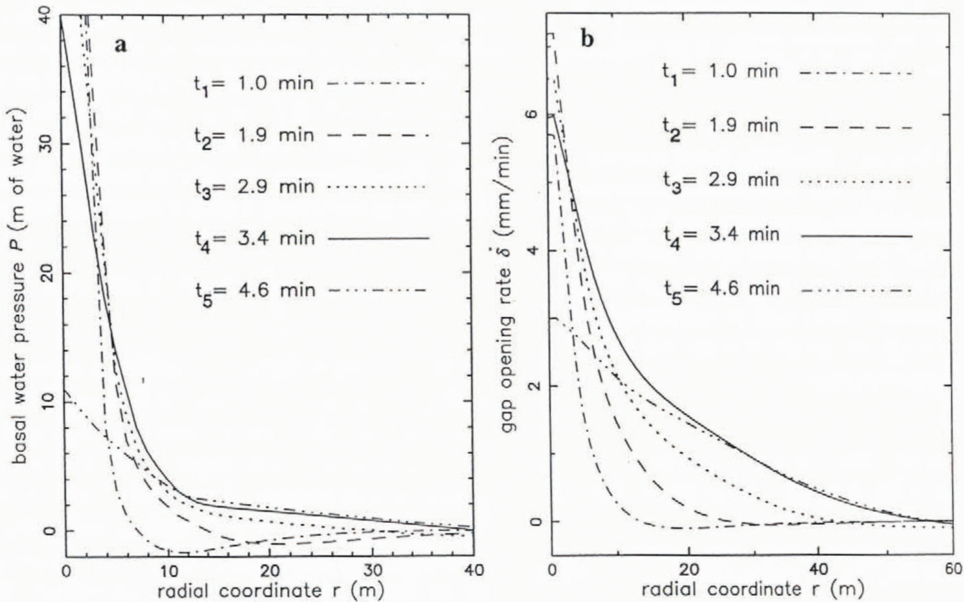
The water flux qw(ro,t)is obtained from Equation 19, based on  from Equation 17. Input to Equation 17is a series of empirical pressure distributions P(r.ti)constructed from borehole information from the pressure propagation experiment (section 8), at five specific times ti( Table 3) as follows. At t =1.9 min after breakthrough the leading edge of the pressure wave reaches 91–1 at r= 14 m. We construct a curve P(r,1.9min) (shown in Eigure 22 as the equivalent zw(r, 1.9 min)) that starts at r = R(1.9min) = 84m, that is generally concave upward, and that descends to zero zw(14m, 1.9 min) =0, at r=R (1.9min) = 14 m (radial distance to 91–1). In constructing the curve near r= 0 the simplest curve form is used — a linear decrease in zwwith r— rather than a parabolic form as suggested by Figure 21a; this is done because (i) there is insuffficient information to construct a parabolic curve; (ii) the parabolic form is not an essential feature of solutions of Equations (17)–(20); and (iii) the output
 is not sensitive to the detailed form of the input pressure near r= 0. To the curve so constructed for r > R, a negative tail is added for r > R,of the form
 , where A is chosen so that the slope of the main curve and tail match at r = R, and where Kis adjusted as explained below. This form of the tail is suggested by Figure 21a. The same procedure is used to construct a curve zw(r3.4 min), at the time of wave arrival at 89–3; this curve is in addition constrained by the observed zw(14 m, 3.4 min) = 2 m from Figure 19b. A later curve, at t= 4.6 min, is constructed from Figure 19b. A later cureve, at t = 4.6 min, is constructed from zw(ro, 4.6 min) = 11 m, zw(14 m, 4.6 min) =2.4 m, and zw(39 m, 4.6 min) =0.3 m, the leading edge of the wave being extrapolated to R(4.6 min) =44 m by following the same leading-edge slope as for the zw(r, 3.4 min) and zw(r, 2.9 min). The set of empirical curves zw(r,t)is shown in Figure 22a.
Empirical calculation of gap-growth rate based on observation of water-pressure distribution P(r, t) in the pressure-pulse propagation experiment, (a) Empirical curves of P(r. ti) at selected times tias indicated, based on observations and assumptions noted in the text (section 9c). (b) Corresponding gap uplift rales  , based on Equation (17). These are used to calculate by integration the volume of water stored at the different times (see text).
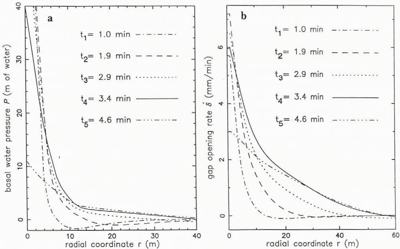
Evaluation of the gap-opening model: model of water stored in basal gap vs volume estimated from borehole water-level drop (WLD)
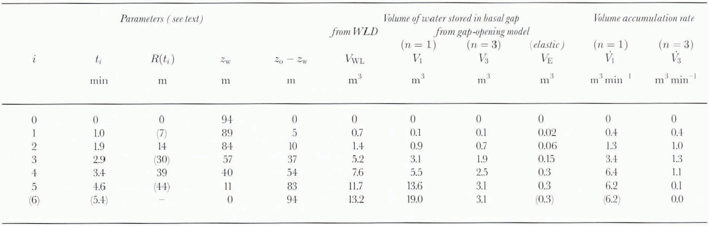
The model calculation is carried out as follows. At each time ti, for which a curve zw(r, t i)has been constructed as described above,  is calculated from Equation 17, after first adjusting the “tail constant” K(see above) such that the global force-balance condition is satisfied:

(This is a force-balance condition because Zwis proportional m pressure Prelative to flotation.) In both Equations (25) and (17) the upper limit of integration r→ 221E; is replaced by a practical upper limit r= L =50 m for purposes of calculation, Then qw(roti), is calculated from Equation 19for r = ro= 0.05 m. and with the upper limit of integration taken to be R(ti)rather than ∞ The value of η Iin Equation 17is chosen as follows. The secondary-creep-rate value, from the 0°C flow law of Reference PatersonPaterson (1994, p.97)for effective stress τ = 2.8 bar, is corrected by a factor 10−2to represent the primary (transient) creep rates that occur at the very low strains involved (10−4for uplift of a few millimeters over dimensions of tens of meters) giving η I=0.94 × 10¹⁰Pa s. The importance of the transient creep viscosity in this type of calculation was pointed out by Reference WeertmanWeertman (1970, p. 73). The validity of a correction factor ≲10–2can be seen in the results of a typical ice-creep test shown in Figure 23. The effective shear stress value r= 2.8 bar is about one-third of the initial overpressure P0= 9.4 bar applied near r= 0 to the base of the ice at breakthrough; the factor of about one-third is estimated from a study of the complete stress solution on which Equation 17is based.
Results of a creep test on ice, showing the magnitude of the initial transient crep rate in relation to the steady-state creep rate. (a) Creep displacement vs time over the 6d period of the test, reaching approximately steady state at a creep rate of 0.0075 mm d−1. (b) Enlarged plot of the initial 24 h of the test, whowing a creep rate of 0.75 mm d−1at a time 0.59 h aftr the start of the test. This is part of test 3 by M. Jackson and B. Kamb (unplblished information), carried out on and ice-core specimen from the site III area.

The calculated qw(r0, ti) values are listed in Tanle 3 in terms of  , which is the total volumetric accumulation rate of water in the gap, at time ti. A smooth curve is drawn through the
 values and is integrated from t= 0 to tito obtain, by Equation 24, the total accumulated volume of water V1(Ti)given by the model. Alongside the values of V1(ti)in Table 3are listed the observational values of injected water volume, VWL(ti), from Equation 23.
An estimate of the effect of the non-linear rheology of ice on the model results can be obtained by treating η Iin Equation 17as a non-Constant quantity proportional to τ–(n–1) where nis the exponent in the non-linear flow law for secondary creep and τ is the effective stress equal to about one-third of the water pressure, relative to flotation, at r≅ 0. This treatment is based on the experimental observation that the transient creep rate is proportional to the secondary creep rate (Reference Sunder and WuSunder and Wu. 1990, p. 271). Thus we can take η Ito be given by

where η ois the value of η Iused in the linear treatment above. Each  (ti) value from the linear treatment then corresponds via Equation 17to a value
 non-linear viscosity (n= 3),
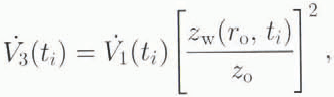
and can be time-integrated as before to give V3(ti). Values of  and V3(ti)are listed in Table 3. Comparison of the VWL(ti), V1(ti)and V3(ti)values in Table 3shows that the gap-opening model as formulated above is able to account for the oobservationally based water volumes VWLto within better than an order of magnitude, which, in view of the numerous approximations and sources of uncertainty in the calculation, gives support to the model.
The most imponderable source of uncertainty in applicability of the model as formulated in Equations (17)–(21) arises from the fact that the gap at the base of the ice overlies not a smooth, hard bedrock surface, as Figure 20suggests, but a rough granular surface of more-or-less loose till particles more-or-less imbedded in a weak fine-granular matrix, the upper surface of the subglacial till (unpublished information from S. Tulaczyk and others. 1996). It is possible that during breakthrough, in the outrush of water from the bottom of the borehole and out through the gap, channels of some kind are cut into the till, and granular material from the till is moved outward through the gap and possibly de-posited along the way. If so, substantial modifications of the treatment in Equations (17] (21), perhaps along the lines developed by Reference Walder and FowlerWalder and Fowler (1994), would probably be required.
9d. Grathents in basal water pressure
The argument in section 9b against the existence of a simple or braided gap-conduit system with gap thickness δ≳ 1 mm is strongly reinforced by independent evidence from the observed borehole water levels after breakthrough. The evidence is in the extent of variation of the water levels from hole to hole (section 3). If we compare the water levels in boreholes less than about 400 m apart, which excludes comparison of holes drilled in different seasons because the ice movement separates them by ≳ 400m in absolute position, we find water-level differences of 6,7 and 15 m between clusters of holes about 150–300 in apart (boreholes of 1988,1989 and 1995), and we find several examples (mainly in 1988) of water-level differences of 5–13 m between individual holes within clusters. 40–10 m араrt. ( Table 1; Fig. 4). These differences are much greater than the ± 1 m estimated measurement error. If a gap-conduit system with δ≳ 1 mm were present in the undisturbed basal water system, and had adequate hydraulic compliance as demonstrated by the uptake of water in breakthrough and pumping tests (section 6), then the water levels observed in the boreholes would represent natural pressures in that conduit system. The differences in water level, over horizontal distances ranging from 15 to 300 m. would then correspond to local hydrostatic grathents ranging from Γ = 0.02 to 0.6. Such grathents are very much greater than the regional hydraulic grathent Γ of about 0.002. Thus if the basal water system is a w idely distributed gap-conduit system as visualized in section 9a, the local water fluxes in this system must be very much larger than the regional flux that transports the integrated basal meltwatcr from upstream. For example, a grathent Γ = 0.1 in a conduit system with δ = 4.3 mm and ϕ = 0.5 would produce, according to Equation 1, a flow velocity u w= 35 cm s−1, compared to the regional flow of 0.7 cm s−1(estimated in section 7). The large water fluxes would refluire large sources and sinks of water on a horizontal scale ∼100 m.
Sources could conceivably be warm areas of the bed. warmed by extra frictional heating where the basal lubrication mechanism is for some reason reduced in effectiveness, but the magnitude is staggering: to accumulate a flow of 35 cm s −1in the above example, over a horizontal distance of 200m, would require basal melting at the absurd rate of 230 m a−1. There is no reasonable way to provide a sink for this water. The situation for δ = 1.7 mm, as evaluated from breakthrough (section 9a), would be less extreme, but it would still involve excessive local water fluxes and basal melting rates. Also, the model associates areas of high frictional heating with areas of high basal water pressure, which is opposite to what is expected — that high water pressure results in low friction.
The severe problem posed by the high local hydraulic grathents can be eliminated only by ruling out any natural gap-conduit system with δ ≅ 1mm, in agreement with the conclusion in section 9b.
It is, however, possible to retain a narrow gap or “water film” of thickness δ ≅ 0.1 mm, through which basal water can be transported slowly, under relatively high local hydraulic grathents. For example, if the basal melting rate is 26 mm a −1(corresponding to a basal shear stress of 0.2 bar and a basal sliding speed of 1.2 md−1), and if the basal mellwatcr flux that accumulates over a flow path ∼100 m long is transported under the same hydraulic grathent as before, Γ = 0.1, then the film would have δ = 0,3 mm. Although the existence of such a film, bridged by coarser grains from the till as visualized bv Reference AlleyAlley (1989b. p. 119), seems quite reasonable, it is not necessarily required as part of the basal water system, because Darcy flow through the till is marginally able to transport locally the small meltwater fluxes generated locally. Thus, for example, a 10m thickness of till with hydraulic conductivity 10 −8ms −1is able to transport the meltwater generated by a basal shear stress of 0.2 bar over a distance of 50 m with a drop of 20 m in hydraulic head.
9e. Canal model
The thin water film visualized in section 9d, with δ≲ 1 mm, in combination with the poor aquifer provided by the bulk till, is quite incapable of transmitting the regional water flux from basal melting upstream, which must cm average be transported down the small regional hydraulic grathent. Therefore there must exist, in addition to any water film, a system of conduits carrying the regional flux and receiving local meltwater from the film and from the bulk aquifer. These conduits arc not classical R-tunnels, according to the observational argument in section 9 and the theoretical arguments of Reference Walder and FowlerWalder and Fowler (1994). The conduits may, however, be of the type called “canals” by Reference Walder and FowlerWalder and Fowler (1994, p. 5, 9): wide, shallow channels, ∼0.1 m deep, incised by erosion into the till, with flat till floor and flat ice roof, of width unspecified but much greater than depth, Waldcr and Fowler (1994) argue theoretically that under the ice stream such canals should form a distributed, interconnected (braided), multi-channel network, non-arborescent, and stable against condensation to a single-channel system. These features differ greatly from those of R-tunnel systems. The apparent need for a canal system as a principal component of the basal water system raises a number of issues in relation to our observations:
(1) If there are canals, what is the local water pressure in them? It should be limited from above by the deepest observed water level, 117 m in hole 92–1. below flotation by about 16 m. (This disregards the deeper levels 119 and 125 m recorded for a short time in the abrupt drop on JD 24 in Figure 15.) How close this value was to the canal water level depends on factors discussed in item 3 below. The fairly abrupt cut-off in initial water-level values at about 116 m, or in basal effective pressures at 1.6 bar, suggests that this cut-off is the actual water level or effective pressure in the canal system locally. From the argument in section 9d we expect the spatial variation of pressure in the canal system to be very much smaller than the observed variation of water levels.
(2) Where arc the inferred canals? In principle, one could hope to locale them from a map of observed water levels in an array of boreholes on a spacing ∼50m; the deepest levels should in general be closest to the canals. There is a question whether the map for this purpose should show the boreholes in their correct positions relative to the ice. as in Figure 4a, or relative to the bed, which involves replotting the boreholes in positions displaced by the proper multiple of the yearly motion, because the water-level data in Figure 4aare from four different years (field seasons). In neither type of map is the borehole array well suited to locating any canals. A possible indication of closeness to a canal is seen in the relation between the group of three boreholes 89–1, −2, −3 (with deep water levels) and the group 89–4, −5, −6 (with shallow levels) (see Figs 2a and 4a). From this and other such indications in Figure 4we infer tentatively that canals are spaced ∼50–300 m apart. Reference Walder and FowlerWalder and Fowler (1994)do not predict theoretically the lateral spacing of canals nor the spatial scale of reconnection in the braided pattern. They do give an indication of the expected canal thickness and width (∼0.1 m, ≫ 0.1 m), but our observations do not provide a basis for checking on this.
(3) What sort of hydraulic connections did the boreholes make with the contemplated canal system? The spread of initial water levels from 117 m to shallower depths indicates that most of the connections were so narrow and/or lengthy that the apparent basal water pressures indicated by the water levels were raised substantially above the water pressure in the canals. The amount by which they were raised should be proportional to the flux of water moving through the connecting passageway (which presumably is along the ice/till contact), but we have no way to estimate separately the magnitude of the flux or the hydraulic impedance of the connection. Presumably the flux is fed by water remaining in the borehole and the open gap after completion of break-through. On the assumption that the canal system has a high hydraulic compliance, we surmise that an indication of connection to it during breakthrough would be an abrupt increase in the water-level drop rate. Such behavior is perhaps seen in Figure 3b. One might expect that the more rapid the drop (or the shorter the drop time or the time constant Tin Table 1), the better the connection to the canal system and hence the deeper the water level reached in breakthrough, but the data in Table 1show no correlation between these values; however, the range of water-level values for which we have Tdata in Table 1is inadequate.
(4) The straightforward interpretation of the salt-tracer experiment (section 7) in terms of the gap-conduit model (section 9a) becomes more complicated and uncertain in the canal model. Presumably the salt cloud spread outward from the injecting borehole in the newly opened gap until it entered a canal via a connection. In order for a big electri-cal-conductance signal to be picked up between the electrodes dow nstream, a salt-carrying canal had to pass near both boreholes of the gate, because the salt presumably remained in the canal system once it had entered. For the canal model there is a need to explain how the inter-electrode resistance remained low for 10 h after the initial drop (Fig. 18a), because at the transport speed in the tunnel (∼5 cm s−1, from the Manning formula for a canal 10cm deep at the regional hydraulic grathent of 0.002) the salt would have been carried downstream 1.8 km in that time. However, the salt solution may have entered the canal system only slowly, through the connection, and continued to do so for 10 h. With this possibility available, the salt-tracer experiment does not provide a very clear lest of the canal model.
10. Conclusion
(1) The gap conduit model of the basal water system, with gap width δ = 2 mm between ice sole and bed, accounts at least roughly for the behavior of borehole water levels on drill breakthrough to the basal water system (section 3), and with δ = 4 mm it accounts for the results of a salt-tracer experiment (section 7) in relation to the transport of basal meltwater from upstream (section 9a). (This type of model was introduced by Reference WeertmanWeertman (1970), who called it the “water layer” model or the “punctured water sheet” model.)
(2) However, the existence of such a gap-conduit system in nature (before disturbance by boreholes) is ruled out by the way a pressure pulse injected into the basal water system at breakthrough propagates outward (sections 7 and 9b), and by the large hole-to-hole variation of measured basal pressure, which if present in a gap-conduit system with δ = 2 or 4 mm would result in unacceptably large local water fluxes, much larger than the regional flux that transports basal meltwater from upstream (section 9d).
(3) An alternative view of the breakthrough process, incorporated into a “gap opening” model, pictures the injection of water as being accommodated by a small lifting of the ice mass near the borehole, opening a gap .3 or 4mm wide at the ice bed contact, where no comparable gap had existed before breakthrough. A quantitative gap-opening model (section 9c) is able to account roughly for the volume of water injected in a breakthrough event, which means that the gap-opening process works and is a valid substitute for the gap-conduit model in accounting for the breakthrough observations.
(4) Although we have not obtained direct borehole access to it, there probably exists a through-going system of water conduits capable of transporting basal meltwater down the regional hydraulic grathent (Γ ∼ 0.002) (section 9e). The only currently viable candidate for these conduits is the “canal”, a theoretical concept of Reference Walder and FowlerWalder and Fowler (1994). Our basal water-pressure data suggest that the canals form a distributed network with spacing ∼50–300 m. With some complications the canal model can be seen as compatible with the salt-tracer experiment (sections 7 and 9e).
(5) The wide scatter of water levels in boreholes that have connected to the basal water system as almost all have . from near flotation to as much as 17 m below flotation, is due to varying quality of the connection along the ice bed interface from borehole to canal. Six or eight boreholes probably did not make connection to the canal system, although they were in connection with a gap opened up by the applied overpressure, a non-natural part of the basal water system.
(6) The water pressure in the canals is about l.6 bar below the ice overburden pressure (section 9e). This low effective pressure (1.6 bar) is probably responsible for the rapid ice-stream motion, either by basal sliding or by shear deformation of the till that underlies the ice.
(7) The ice overburden pressure can be calculated to an accuracy of about 0.3 bar from data on ice density vs depth locally and in the Byrd core hole (section 4).
(8) The pore pressure in the till, and the water pressure in a thin (δ≲ 0.1 mm) water film that probably is present somewhat discontinuously along the ice/till contact, cannot be measured in an open borehole, but in principle can be measured once the borehole has frozen up, once passageways connecting with canals have become closed, and once enough time has elapsed for pressure equilibration. The equivalent water levels observed in this way were in the range 100–112 m depth and varied extensively with time over this range on time-scales from diurnal to more than a year.
(9) The extent of correlation between time variations recorded by different pressure sensors from no correlation between sensors 500 m apart to good correlation with some exceptions, between sensors 25m apart indicates that the sensor signals are in general real indications of basal water pressure (probably till-pore pressure as noted above), and that the natural distance scale for lateral variations in (pore) pressure is ∼100 m or al times as small as ∼10 m section 5). Thus some of these variations are probably local effects originating in the till (and water film), due perhaps to local changes in the basal melting rale as the mechanical conditions of the till vary, or to the opening or closing of basal cracks in the ice. Other, longer-scale variations, and particularly the highly correlating diurnal fluctuations, probably originate in the canal system, from which they are communicated to the till-pore water and the water film. However, the origin of these numerous variations is not known in any detail.
(10) The occurrence of interspersed positively correlating variations and negative, anticorrelating variations in the 1995 pressure records from boreholes 89–4 and 91–1 (section 5) is probably at least somewhat related to the anticor-relations observed by Reference Murray and ClarkeMurray and Clarke (1995)in pressure records from a subpolar glacier (Trapridge Glacier) in Canada. They interprel the anticorrelations as an indication that when the pressure rises in a low-impedance basal water conduit such as an R-tunnel, the pressure in the adjacent part of the bed unconnected to the conduit must fall to maintain the vertical force balance supporting the (fixed) ice overburden; they interpret switching back and forth between correlation and anticorrelation in the pressure records as due to a switching back and forth between a connected and unconnected condition in one of the boreholes. Direct applicability of this interpretation to our pressure records in Figures 14 and 15 is doubtful, because the records do not distinguish one borehole as connected and the other as unconnected. At the time of original breakthrough, the initial water levels (112 vs 99m) indicated that hole 91–1 was heiler connected than hole 89–1, according to the interpretation in paragraph 5 above, bin this distinction had disappeared by the time-frame of Figure 15, when the pressure levels in the two holes were approximately the same. Nevertheless, there is probably some underlying relationship between the pressure anticorrelations in the two glacier systems.
(11) The diurnal pressure fluctuation, which we have observed several times (Fig 11and 12), might be due to the tide in the Ross Sea (Reference Harrison, Echelmeyer and EngelhardtHarrison and others. 1993), although its phasing and modulation do not seem to support this conclusion (section 5).
(12) The lack of any observed variation in ice-stream motion, when large percentagewise variations in basal effective pressure were observed to be occurring, is a situation somewhat similar to that encountered in Columbia Glacier, Alaska (Reference Kamb, Engelhardt, Fahnestock, Humphrey, Meier and StoneKamb and others, 1994; Reference MeierMeier and others. 1994), where the basal water pressure was consistently high (within 3 bar of flotation) but there was little correlation between variations in pressure and motion, except for diurnal variations. The conclusion reached there may to some extent be applicable here also: that locally observed pressure variations, caused by variations in basal melting or by random local rearrangements of the water conduit system, are mostly averaged out over the long distance scale (coupling length over which basal water pressure is effective averaged in controlling the basal motion Reference Kamb and EchelmeyerKamb and Echelmeyer, 1986). For this to result in the observed constancy of ice-stream motion, the pressure flucuiations at points farther apart than some characteristic distance scale of “localization” short compared to the coupling length should be randomly different and uncorrelated. From this point of view, the observed lack of correlation between the pressure records from boreholes 500 m apart and even at times from boreholes only 25 m apart perhaps makes sense.
Detail of basal water-pressure variation, expressed as water-level depth, at hole 88–3 during (a) 1989–90, and (b) 1900–91.
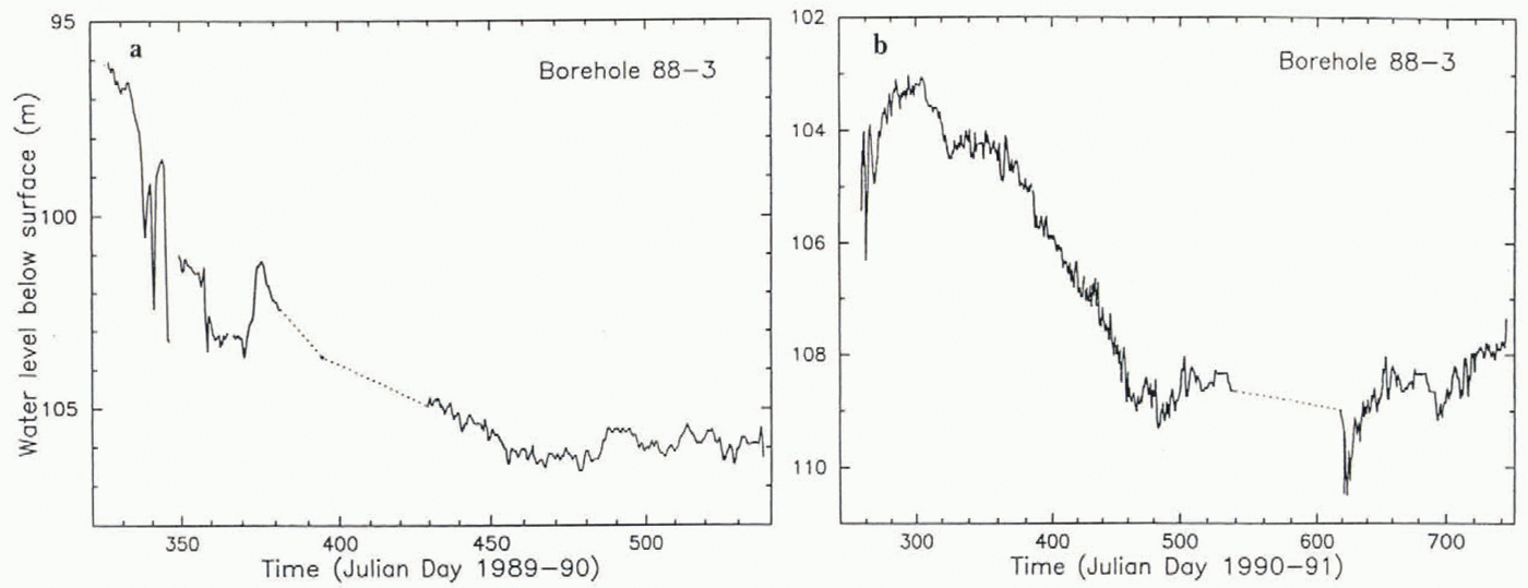
Acknowledgements
We are indebted to many field assistants, camp personnel, and flight crews for help in carrying out the fieldwork for this paper. We thank Dr D. B. Stone and an anonymous reviewer for critical comments on the manuscript. The work was made possible by grants ОРР-8519083, ОРР-9018703 and OPP-9319018 from the U.S. National Science Foundation.