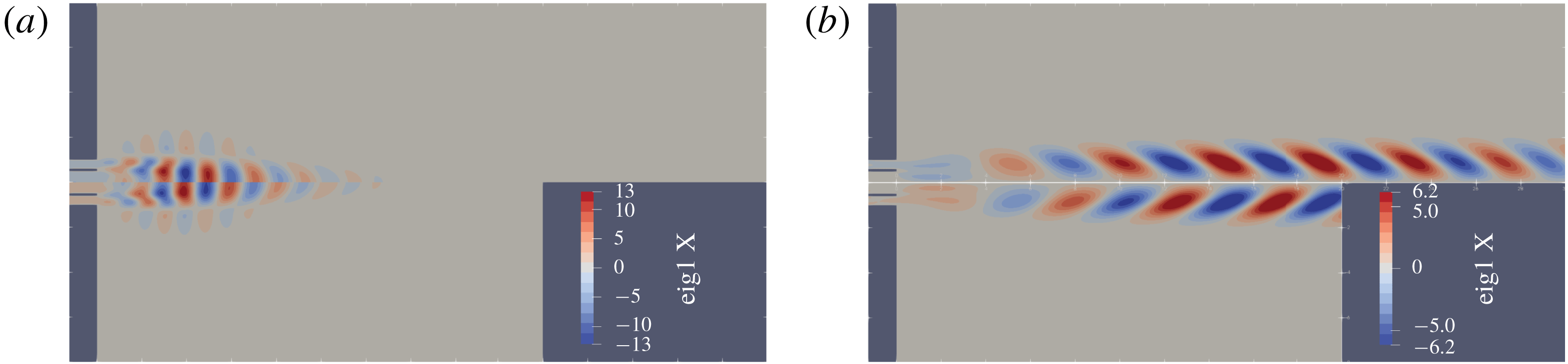
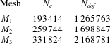
1 Introduction
Coaxial jets are employed in several industrial applications, such as in noise control, mixing processes and energy conversion by combustion. Atomisers, burners and mixers exploit the interpenetration of the two streams as an effective mixing mechanism, since the external jet can destabilise the internal jet and, as a consequence, increase mixing by promoting transition to turbulence, see Villermaux & Rehab (Reference Villermaux and Rehab2000) and the references therein. Several aeronautical applications use coaxial jets to reduce the noise produced by the single jet layout (Williams, Ali & Anderson Reference Williams, Ali and Anderson1969). Swirling jets are often employed in combustors to enhance the stability of flame anchoring thus improving the efficiency of the combustion and reducing the
 $\text{NO}_{x}$
emissions (Lefebvre Reference Lefebvre1998).
Coaxial jets are also interesting to investigate the subcritical transition process in parallel or quasi-parallel flows. Indeed jets, and in particular coaxial jets, exhibit subcritical transition such as the Couette and Poiseuille flows and boundary layers. With respect to the above mentioned flows, this phenomenon is particularly notable in coaxial jets that exhibit a very strong non-normal behaviour (Canton, Auteri & Carini Reference Canton, Auteri and Carini2017). This property makes them ideal for mixing (Schumaker & Driscoll Reference Schumaker and Driscoll2012), especially for low Reynolds number applications (Saiki, Suzuki & Kasagi Reference Saiki, Suzuki and Kasagi2011).
The mixing and noise-generation properties of coaxial jets are strongly related to their stability since the flow behaviour depends on the dynamics of large-scale coherent vortical structures produced by the amplification of external perturbations. Jets, and coaxial jets in particular, are known to be convectively unstable (Chomaz Reference Chomaz2005), with large amplification rates (Garnaud et al.
Reference Garnaud, Lesshafft, Schmid and Huerre2013a
,Reference Garnaud, Lesshafft, Schmid and Huerre
b
; Canton et al.
Reference Canton, Auteri and Carini2017). The instability modes are usually referred to as varicose, when the unstable perturbation is axisymmetric, sinuous, when the perturbation appears as a sinusoidal transverse wave propagating along the jet axis and they have azimuthal wavenumber
 $|m|=1$
, helical, when the perturbation resembles a helix with wavenumber
 $|m|>1$
. When swirl is present in the jet, helical modes are usually characterised by a spiral motion. This motion is termed co-winding, if the helix winds in the same direction of the rotation of the jet, otherwise they are termed counter-winding or retrograde. Several studies in the past have investigated the linear stability of jets in the incompressible and compressible regimes. The inviscid stability of parallel jets was investigated by Batchelor & Gill (Reference Batchelor and Gill1962). They found a sinuous unstable perturbation with
 $m=1$
for a top-hat velocity profile, for which the velocity is constant in the central region and then goes rapidly to zero, but noticed a high impact of the velocity profile on the stability properties of the flow. Crighton & Gaster (Reference Crighton and Gaster1976) emphasised the importance of non-parallel effects and of the nozzle region. These effects were fully taken into account by Garnaud et al. (Reference Garnaud, Lesshafft, Schmid and Huerre2013a
,Reference Garnaud, Lesshafft, Schmid and Huerre
b
) who showed the inadequacy of a modal stability analysis in understanding the stability of the flow, while pointing out the importance of convective instability.
The swirling jet has been investigated theoretically and numerically exploiting different base flows: the Batchelor vortex (Leibovich & Stewartson Reference Leibovich and Stewartson1983; Khorrami Reference Khorrami1991; Delbende & Rossi Reference Delbende and Rossi2005), a standard or screened Rankine vortex (Loiseleux, Chomaz & Huerre Reference Loiseleux, Chomaz and Huerre1998; Gallaire & Chomaz Reference Gallaire and Chomaz2003a ) or other flows (Martin & Meiburg Reference Martin and Meiburg1994, Reference Martin and Meiburg1996; Loiseleux, Delbende & Huerre Reference Loiseleux, Delbende and Huerre2000; Gallaire & Chomaz Reference Gallaire and Chomaz2003b ). The reported results show that instabilities are mainly convective, related to the Kelvin–Helmholtz and centrifugal mechanisms. A stability criterion for the centrifugal instability has been formulated for vortices by Leibovich & Stewartson (Reference Leibovich and Stewartson1983), then extended by Billant & Gallaire (Reference Billant and Gallaire2013) to swirling-jet flows.
Most of the experimental activity on swirling round jets has been carried out for moderate to high Reynolds numbers, see Örlü & Alfredsson (Reference Örlü and Alfredsson2008) and the references therein. More relevant to the present work are experiments in the low Reynolds number range. Loiseleux & Chomaz (Reference Loiseleux and Chomaz2003) considered two different Reynolds numbers,
 $740$
and
 $1490$
. For low swirl, the flow behaviour is similar to that observed for a non-swirling jet, namely it is dominated by axisymmetric perturbations whose nonlinear evolution first leads to vortex roll up and then to vortex pairing. A successive instability of the braid connecting to successive vortices, similar to that observed for a non-swirling jet but featuring corotating vortices, rapidly leads to turbulence. For higher swirl numbers in the range
 $(0.6,1)$
, the flow is dominated by the wavenumber
 $m=+2$
. For
 $1\leqslant S_{\mathit{LC}}\leqslant 1.3$
, strong interaction between the axisymmetric mode and the
 $m=+2$
mode is observed, leading to the emergence of the
 $m=+1$
mode. Vortex breakdown is observed for
 $S_{\mathit{LC}}\geqslant 1.3$
. Experiments carried out by Liang & Maxworthy (Reference Liang and Maxworthy2005) for a Reynolds number
 $Re=1000$
showed two different regimes before vortex breakdown. Results similar to those by Loiseleux & Chomaz (Reference Loiseleux and Chomaz2003) are reported in the low swirl regime. In contrast, for intermediate swirl
 $S_{\mathit{LM}}\gtrsim 0.6$
, the initial part of the flow is dominated by helical modes with wavenumbers
 $m=+2$
and
 $m=+3$
. For swirl numbers higher than
 $0.83/0.86$
vortex breakdown is observed. We note in passing that the definition of swirl number
 $S_{\mathit{LC}}$
and
 $S_{\mathit{LM}}$
in the two works is different and different from the definition adopted here, so that the thresholds are not directly comparable.
The theoretical investigation of the stability properties of coaxial jets is more recent. With respect to the round jet, coaxial jets are characterised by several independent parameters, the outer-to-inner ratio
 $R_{D}$
, the non-dimensional thickness
 $s$
of the wall separating the two incoming flows, the Reynolds number
 $Re$
, the ratio between the maximum axial component of the velocity of the outer and inner jets
 $r_{u}$
, the swirl numbers of the inner and outer jet. Michalke (Reference Michalke1999) first analysed the inviscid spatio-temporal stability of a parallel annular jet, with possible backflow in the jet core. He found that an absolute instability can arise only for the perturbation with azimuthal wavenumber
 $m=+1$
. If a backflow is present, the absolute instability occurs with or without swirl, while a swirl is necessary if there is no backflow. Talamelli & Gavarini (Reference Talamelli and Gavarini2006) considered the inviscid linear stability analysis of incompressible coaxial jets mimicking the presence of a blunt wall separating the two jets by a low-speed wake in the velocity profile. They found an absolute instability limited to negative or small positive values of the minimum velocity imposed in the wake. They also found that the amplification factor grows as the shear layers thin out. Their findings were substantially confirmed by a global stability analysis by Canton et al. (Reference Canton, Auteri and Carini2017) showing that the flow is absolutely unstable for Reynolds numbers above 1356 when a blunt separating wall is present. Canton et al. (Reference Canton, Auteri and Carini2017) also showed that the subcritical base flow is convectively unstable with huge amplification of the initial perturbations. Weller-Calvo, Fontane & Joly (Reference Weller-Calvo, Fontane and Joly2015) extended the analysis carried out by Talamelli & Gavarini (Reference Talamelli and Gavarini2006) to account for a swirl motion.
An extensive experimental activity has investigated coaxial jets. Several works investigated the fully turbulent coaxial jets both without (Champagne & Wygnanski Reference Champagne and Wygnanski1971; Buresti, Talamelli & Petagna Reference Buresti, Talamelli and Petagna1994; Sadr & Klewicki Reference Sadr and Klewicki2003) and with swirl (Ribeiro & Whitelaw Reference Ribeiro and Whitelaw1980; Champagne & Kromat Reference Champagne and Kromat2000), reporting mainly the mean flow properties and turbulence statistics. More germane to the present investigation are experiments carried out for low and moderate Reynolds numbers, where details of the instability and transition process are available. In their experiments, Dahm, Frieler & Tryggvason (Reference Dahm, Frieler and Tryggvason1992) investigated non-swirling jets for three moderate Reynolds numbers (
 $1333$
,
 $5867$
,
 $10\,668$
). For small velocity ratios they observed a sinuous instability with wavenumber
 $m=\pm 1$
while for
 $r_{u}\geqslant 0.71$
they observed the development of an axisymmetric instability. For the higher velocity ratio tested,
 $r_{u}=1.14$
, they observed lock-in of the perturbations in the outer and inner shear layers. This phenomenon was observed also by Tang & Ko (Reference Tang and Ko1994) for
 $Re=1700$
and
 $r_{u}=3.33$
. The results presented by Wicker & Eaton (Reference Wicker and Eaton1994) show a different behaviour. For low velocity ratios,
 $r_{u}\leqslant 0.71$
, they observed the development of axisymmetric structures, before further instabilities break the symmetry, while for
 $r_{u}=1.23$
and
 $1.45$
they observed a helical instability developing in the central jet. When forcing is applied, only axisymmetric vortex rings are produced, with a peak in the response for a Strouhal number
 $St=0.5$
. Rehab, Villermaux & Hopfinger (Reference Rehab, Villermaux and Hopfinger1997) observed that a recirculation region forms for velocity ratios higher than approximately
 $8$
. For lower velocity ratios, but still quite high with respect to those investigated here, they found the outer shear layer dominating the instability process. An important appreciation of the role of the velocity ratio was provided by Segalini & Talamelli (Reference Segalini and Talamelli2011), who found three different behaviours: for low velocity ratio, the frequency of the instability depends on the velocity of the internal jet, for high velocity ratios it depends on the velocity of the external jet, while for intermediate velocity ratios it depends on both.
The transition process in incompressible coaxial jets without swirl has been investigated also numerically by da Silva, Balarac & Métais (Reference da Silva, Balarac and Métais2003), Balarac & Métais (Reference Balarac and Métais2005), Balarac, Métais & Lesieur (Reference Balarac, Métais and Lesieur2007) without and with external forcing. In particular, they found that the thickness of the boundary layer at the nozzle exit has a strong influence on the instability process. As one may expect, the thinner the boundary layer the stronger the instability. For low velocity ratios they found the initial instability dominated by a sinuous perturbation with wavenumber
 $1$
. A secondary instability is found where longitudinal vortices are formed in the braid between successive primary vortices that rapidly lead to transition. A linear spreading of the jet is observed after transition. When axisymmetric forcing is applied, strong axisymmetric vortices are formed. Azimuthal excitation leads to the appearance of relatively short wavelengths undulations in the main vortices whose wavenumber is selected by forcing (Balarac et al.
Reference Balarac, Métais and Lesieur2007).
To clarify the instability mechanisms that eventually lead to transition in coaxial jets, even without an absolute instability, and in particular to assess the role that inflow perturbations play in this process, in this work, we investigate the harmonic response of non-swirling coaxial jets in a region of the space of parameters
 $Re-r_{u}$
where the system is globally stable. Then the influence of the swirl parameter
 $S$
of the outer stream is assessed on the columnar state of coaxial jets with unitary velocity ratio. The base flow is assumed axisymmetric and the homogeneity of the azimuthal coordinate
 $\unicode[STIX]{x1D703}$
allows us to exploit the Fourier decomposition of the perturbation fields to obtain the linear dynamics of the system as a combination of the independent evolution of the modes associated with different azimuthal wavenumbers, without resorting to time-stepping techniques. With respect to Canton et al. (Reference Canton, Auteri and Carini2017), we adopt a different perspective. Firstly, we analyse the response of the system to inflow disturbances, since this is probably one of the most likely ways disturbances enter the flow field. Moreover, as shown by Garnaud et al. (Reference Garnaud, Lesshafft, Schmid and Huerre2013b
), the responses of the flow to optimal inlet forcing and optimal volume forcing are qualitatively very similar at the same frequency. Secondly, we restrict our analysis to lower subcritical Reynolds numbers, to avoid the huge amplifications observed for Reynolds numbers as low as
 $1000$
. Thirdly, we analyse the response of the base flow to both axisymmetric and non-symmetric forcing. Fourthly, the effect of swirl is here considered for the first time. Three-dimensional nonlinear simulations with perturbed inflow conditions are also performed in order to verify the validity of the assumptions made, to verify the results obtained and the predominance of the preferred response. Both dynamic-mode decomposition and Fourier decomposition of time snapshots are used to describe the global dynamics of the system and to compare the structures emerging in the nonlinear system with the prediction of the linear non-modal analysis.
The paper is organised as follows. The flow configuration is presented in § 2. The non-modal harmonic response is recalled, and the numerical approach is described in § 3. The influence of the velocity ratio
 $r_{u}$
and the swirl parameter
 $S$
on the base flow and on the harmonic response of axisymmetric base flow is presented in § 4 and § 5, respectively. The results of fully three-dimensional perturbed direct numerical simulations are presented in § 6. Conclusions are drawn in § 7.
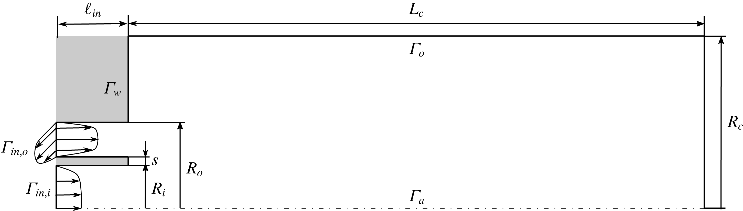
Azimuthal slice of the three-dimensional axisymmetric domain, coinciding with the numerical domain used for the response analysis of the axisymmetric base flow. Figure not drawn to scale.

2 Flow configuration
The incompressible flow produced by two cylindrical coaxial jets is considered here. The reference length is chosen as the diameter
 $\widetilde{D}_{i}$
of the inner pipe and the reference velocity as the maximum of the inner axial-velocity profile,
 $\widetilde{U}_{a}$
. A slice of the numerical domain is depicted in figure 1. The outer-to-inner ratio of the pipe diameters is
 $R_{D}=2.0$
, the non-dimensional thickness of the septum is
 $s=0.1$
. The length of the inlet pipes is set to
 $\ell _{in}=2.5$
. The length and the radius of the numerical domain are set to
 $L_{c}=60.0$
and
 $R_{c}=8.0$
(Canton et al.
Reference Canton, Auteri and Carini2017). The Reynolds number is defined as
 $Re=\widetilde{U}_{a}\widetilde{D}_{i}/\widetilde{\unicode[STIX]{x1D708}}$
, where
 $\widetilde{\unicode[STIX]{x1D708}}$
is the constant kinematic viscosity of the fluid. The dynamics of the flow is governed by the non-dimensional incompressible Navier–Stokes equations
 $$\begin{eqnarray}\left.\begin{array}{@{}l@{}}\displaystyle \frac{\unicode[STIX]{x2202}\boldsymbol{U}}{\unicode[STIX]{x2202}t}+\left(\boldsymbol{U}\boldsymbol{\cdot }\unicode[STIX]{x1D735}\right)\boldsymbol{U}-Re^{-1}\unicode[STIX]{x0394}\boldsymbol{U}+\unicode[STIX]{x1D735}P=\mathbf{0},\\ \unicode[STIX]{x1D735}\boldsymbol{\cdot }\boldsymbol{U}=0,\end{array}\right\}\end{eqnarray}$$
where
 $\boldsymbol{U}=\boldsymbol{U}(\boldsymbol{r},t)$
denotes the non-dimensional velocity field, and
 $P=P(\boldsymbol{r},t)$
the non-dimensional reduced pressure field. A no-slip condition is imposed on the wall boundary
 $\unicode[STIX]{x1D6E4}_{w}$
, while a homogeneous Neumann condition is assumed on
 $\unicode[STIX]{x1D6E4}_{o}$
,
 $Re^{-1}\hat{\boldsymbol{n}}\boldsymbol{\cdot }\unicode[STIX]{x1D735}\boldsymbol{U}-P\hat{\boldsymbol{n}}=\mathbf{0}$
. Axisymmetry conditions,
 $U_{r}=0,U_{\unicode[STIX]{x1D703}}=0,\unicode[STIX]{x2202}U_{r}/\unicode[STIX]{x2202}z=0$
, hold on the axis. On the inner and outer inlet boundaries –
 $\unicode[STIX]{x1D6E4}_{in,i}$
and
 $\unicode[STIX]{x1D6E4}_{in,o}$
, respectively – the axial-velocity component is set according to the expressions
 $U_{z,i}(r)$
and
 $U_{z,o}(r)$
used by Canton et al. (Reference Canton, Auteri and Carini2017) to reproduce the mean axial velocity profiles measured by Segalini & Talamelli (Reference Segalini and Talamelli2011). The azimuthal velocity profile
 $U_{\unicode[STIX]{x1D703},o}(r)=S\,U_{z,o}(r)$
at the inflow boundary of the outer jet
 $\unicode[STIX]{x1D6E4}_{in,o}$
is chosen proportional to the axial profile
 $U_{z,o}$
to have a swirl number
 $S$
, defined as the ratio of these two velocity components, independent of the radius. This definition differs from that mainly used in the literature for the single jet, see for instance Liang & Maxworthy (Reference Liang and Maxworthy2005), and also from that adopted by Gallaire & Chomaz (Reference Gallaire and Chomaz2003b
), owing to the difference in the flows.
 $$\begin{eqnarray}\displaystyle & \displaystyle \boldsymbol{U}|_{\unicode[STIX]{x1D6E4}_{in,i}}=U_{z,i}(r)\hat{\boldsymbol{z}}, & \displaystyle\end{eqnarray}$$
 $$\begin{eqnarray}\displaystyle & \displaystyle \boldsymbol{U}|_{\unicode[STIX]{x1D6E4}_{in,o}}=r_{u}U_{z,o}(r)\hat{\boldsymbol{z}}+r_{u}U_{\unicode[STIX]{x1D703},o}(r)\hat{\unicode[STIX]{x1D73D}}, & \displaystyle\end{eqnarray}$$
with
 $$\begin{eqnarray}\displaystyle & \displaystyle U_{z,i}(r)=\tanh [b_{i}(1-2r)], & \displaystyle\end{eqnarray}$$
 $$\begin{eqnarray}\displaystyle & \displaystyle U_{z,o}(r)=\tanh \left[b_{o}\left(1-\left|\frac{2r-(R_{o,1}+R_{o,2})}{R_{o,1}-R_{o,2}}\right|\right)\right], & \displaystyle\end{eqnarray}$$
 $R_{o,1}$
and
 $R_{o,2}$
are the internal and external radii of the annular duct and the two parameters
 $b_{i}$
and
 $b_{o}$
control the thickness of the boundary layers: both values are set to
 $5.0$
as previously done by Canton et al. (Reference Canton, Auteri and Carini2017).
3 Mathematical formulation
The amplification of a small-amplitude stochastic forcing
 $\boldsymbol{f}$
, whose evolution is governed by the linearised system
 $\boldsymbol{u}=\mathscr{R}\boldsymbol{f}$
, can be obtained as a function of the harmonic response of the system, over the whole spectrum of frequencies (Farrell & Ioannou Reference Farrell and Ioannou1996). Boujo & Gallaire (Reference Boujo and Gallaire2015) expressed the ensemble variance
 $$\begin{eqnarray}E={\displaystyle \frac{1}{2\unicode[STIX]{x03C0}}}\int _{-\infty }^{+\infty }\mathop{\sum }_{k}G_{k}^{2}(\unicode[STIX]{x1D714})\,\text{d}\unicode[STIX]{x1D714}={\displaystyle \frac{1}{\unicode[STIX]{x03C0}}}\int _{0}^{+\infty }\mathop{\sum }_{k}G_{k}^{2}(\unicode[STIX]{x1D714})\,\text{d}\unicode[STIX]{x1D714}\end{eqnarray}$$
as a function of the optimal and suboptimal harmonic gains
 $G_{k}$
, defined either as the singular values of the linearised Navier–Stokes operator
 $\mathscr{R}$
or the square root of the eigenvalues of the Hermitian operator
 $\mathscr{R}^{\dagger }\mathscr{R}$
.
The harmonic response of the flow to velocity perturbations at the inflow is investigated by a non-modal analysis of the linearised flow around the steady axisymmetric solution of the Navier–Stokes equations (2.1). Both axisymmetric and non-axisymmetric perturbations are investigated. The continuity of the fields implies that perturbations must be
 $2\unicode[STIX]{x03C0}$
-periodic in
 $\unicode[STIX]{x1D703}$
and therefore they can be effectively represented by their Fourier series
 $$\begin{eqnarray}(\boldsymbol{u},p)(r,\unicode[STIX]{x1D703},z,t)=\boldsymbol{q}(r,\unicode[STIX]{x1D703},z,t)=\mathop{\sum }_{m=-\infty }^{\infty }\boldsymbol{q}_{m}(r,z,t)\text{e}^{\text{i}m\unicode[STIX]{x1D703}}.\end{eqnarray}$$
Since the perturbation
 $\boldsymbol{q}(\boldsymbol{r},t)$
is real, the complex-conjugate symmetry
 $\boldsymbol{q}_{-m}=\boldsymbol{q}_{m}^{\ast }$
holds for the series coefficients. The harmonic response of the system to small-amplitude perturbations is described in the frequency domain by the Fourier transform of the linearised Navier–Stokes equations
 $$\begin{eqnarray}\left.\begin{array}{@{}c@{}}\displaystyle \text{i}\unicode[STIX]{x1D714}\hat{\boldsymbol{u}}+(\boldsymbol{U}\boldsymbol{\cdot }\unicode[STIX]{x1D735})\hat{\boldsymbol{u}}+(\hat{\boldsymbol{u}}\boldsymbol{\cdot }\unicode[STIX]{x1D735})\boldsymbol{U}-Re^{-1}\unicode[STIX]{x0394}\hat{\boldsymbol{u}}+\unicode[STIX]{x1D735}\hat{p}=\mathbf{0},\\ \unicode[STIX]{x1D735}\boldsymbol{\cdot }\hat{\boldsymbol{u}}=0,\end{array}\right\}\end{eqnarray}$$
supplied with homogeneous Dirichlet and Neumann boundary conditions on
 $\unicode[STIX]{x1D6E4}_{w}$
and
 $\unicode[STIX]{x1D6E4}_{o}$
, respectively, and wavenumber-dependent symmetry conditions on the axis. The harmonic forcing at the inflow is introduced as the essential boundary condition
 $\hat{\boldsymbol{u}}=\hat{\boldsymbol{f}}$
on
 $\unicode[STIX]{x1D6E4}_{i}$
. By the linearity of this model, with reference to the series (3.2), the dynamics of the system is obtained as a combination of the independent evolution of the modes with different wavenumbers, governed by the complex equations
 $$\begin{eqnarray}\left.\begin{array}{@{}c@{}}\displaystyle \text{i}\unicode[STIX]{x1D714}\hat{\boldsymbol{u}}_{m}+(\boldsymbol{U}\boldsymbol{\cdot }\unicode[STIX]{x1D735}_{m})\hat{\boldsymbol{u}}_{m}+\left(\hat{\boldsymbol{u}}_{m}\boldsymbol{\cdot }\unicode[STIX]{x1D735}_{0}\right)\boldsymbol{U}-Re^{-1}\unicode[STIX]{x1D6E5}_{m}\hat{\boldsymbol{u}}_{m}+\unicode[STIX]{x1D735}_{m}\hat{p}_{m}=\mathbf{0},\\ \unicode[STIX]{x1D735}_{m}\boldsymbol{\cdot }\hat{\boldsymbol{u}}_{m}=0,\end{array}\right\}\end{eqnarray}$$
where
 $(\hat{\boldsymbol{u}}_{m},\hat{p}_{m})(\boldsymbol{r},\unicode[STIX]{x1D714})$
indicates the contribution of the
 $m$
th wavenumber
 $(\boldsymbol{u}_{m},p_{m})(\boldsymbol{r},t)$
to the perturbation field and the complex operators
 $\unicode[STIX]{x1D735}_{m}$
,
 $\unicode[STIX]{x1D6E5}_{m}$
for axisymmetric fields are obtained by formally replacing the partial derivative
 $\unicode[STIX]{x2202}/\unicode[STIX]{x2202}\unicode[STIX]{x1D703}$
in the original equations with the factor
 $im$
in the transformed equations. The phase velocity of a perturbation with wavenumber
 $m$
and frequency
 $\unicode[STIX]{x1D714}$
is obtained as
 $\unicode[STIX]{x1D6FA}_{m}=-\unicode[STIX]{x1D714}/m$
by explicitly writing the inverse Fourier transform
 $$\begin{eqnarray}\boldsymbol{q}(\boldsymbol{r},t)={\displaystyle \frac{1}{2\unicode[STIX]{x03C0}}}\int _{-\infty }^{\infty }\hat{\boldsymbol{q}}_{m}(r,z,\unicode[STIX]{x1D714})\text{e}^{\text{i}(m\unicode[STIX]{x1D703}+\unicode[STIX]{x1D714}t)}.\end{eqnarray}$$
The harmonic response of the axisymmetric base flow is computed with a finite element solver of the Navier–Stokes equations in cylindrical coordinates, developed starting from the well-validated baseline code resulting from a collaboration between Politecnico di Milano and the Royal Institute of Technology (KTH) (Canton et al.
Reference Canton, Auteri and Carini2017). The discrete form of the fields and the weak formulation of the problem are built on the standard Taylor–Hood
 $\mathbb{P}_{2}$
–
 $\mathbb{P}_{1}$
finite elements of an unstructured triangulation (Dussin et al.
Reference Dussin, Fossati, Guardone and Vigevano2009) of the numerical domain corresponding to an azimuthal slice of the actual domain. The details of the grid are given in Appendix. The axisymmetric flow is computed by Newton’s iteration, while the computation of the harmonic response follows Garnaud et al. (Reference Garnaud, Lesshafft, Schmid and Huerre2013b
). The spectral element code Nek5000 is used for three-dimensional direct numerical simulations. This is a massively parallel, open-source code based on a spatial discretisation by hexahedral spectral elements with Lagrangian tensor-product bases built on Gauss–Legendre–Lobatto points. A second-order fractional step method is used to advance the solution in time, with a backward differentiation formula of second order implicit treatment of the viscous term and a consistent explicit treatment of the nonlinear term in the momentum equation (Fischer, Lottes & Kerkemeier Reference Fischer, Lottes and Kerkemeier2008). The compatible formulation
 $\mathbb{P}_{N}$
–
 $\mathbb{P}_{N-2}$
is used for the velocity and pressure fields, with
 $N=7$
. The initial condition coincides with the axisymmetric base flow used for the harmonic response. Dynamic mode decomposition (Schmid Reference Schmid2010) is used to describe the global behaviour of the perturbed systems by means of Koopman mode analysis.
4 Base flow
The base flow is briefly described as a function of the outer-to-inner axial-velocity ratio
 $r_{u}$
and of the swirl parameter
 $S$
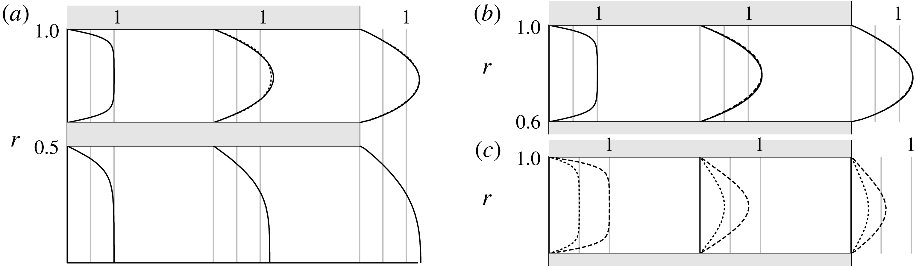
. As observed by Canton et al. (Reference Canton, Auteri and Carini2017), the inlet axial-velocity profile, that mimics the mean velocity measured by Segalini & Talamelli (Reference Segalini and Talamelli2011) at higher Reynolds number, is gradually smeared along the inlet pipe, due to the higher impact of viscous effects at this lower Reynolds number. The thickness of the boundary layer grows along the pipe and the axial velocity profiles qualitatively approach fully developed profiles with the maximum of the axial-velocity profile that increases moving downstream, as shown in figure 2(a,b). The axial velocity profile, normalised with respect to the velocity ratio
 $r_{u}$
, is almost independent of this parameter, as shown in figure 2(b) by superimposing the normalised velocity profiles
 $U_{z}/r_{u}$
corresponding to different values of
 $r_{u}$
. The shape of the azimuthal-velocity profile changes along the outer pipe, while its maximum value decreases, due to viscous dissipation, as shown in figure 2(c) for
 $Re=200$
and
 $r_{u}=1.0$
.
Velocity profile in the inlet pipes. (a) Axial velocity for
 $Re=200$
,
 $S=0$
:
 $r_{u}=1.0$
(solid line),
 $r_{u}=2.0$
(dashed line). In the outer pipe, the velocity is normalised with the maximum value of the axial velocity at the inflow. Axial (b) and azimuthal (c) velocity in the outer pipe for
 $Re=200$
,
 $r_{u}=1.0$
:
 $S=0.5$
(dotted line),
 $S=1.0$
(dashed line).

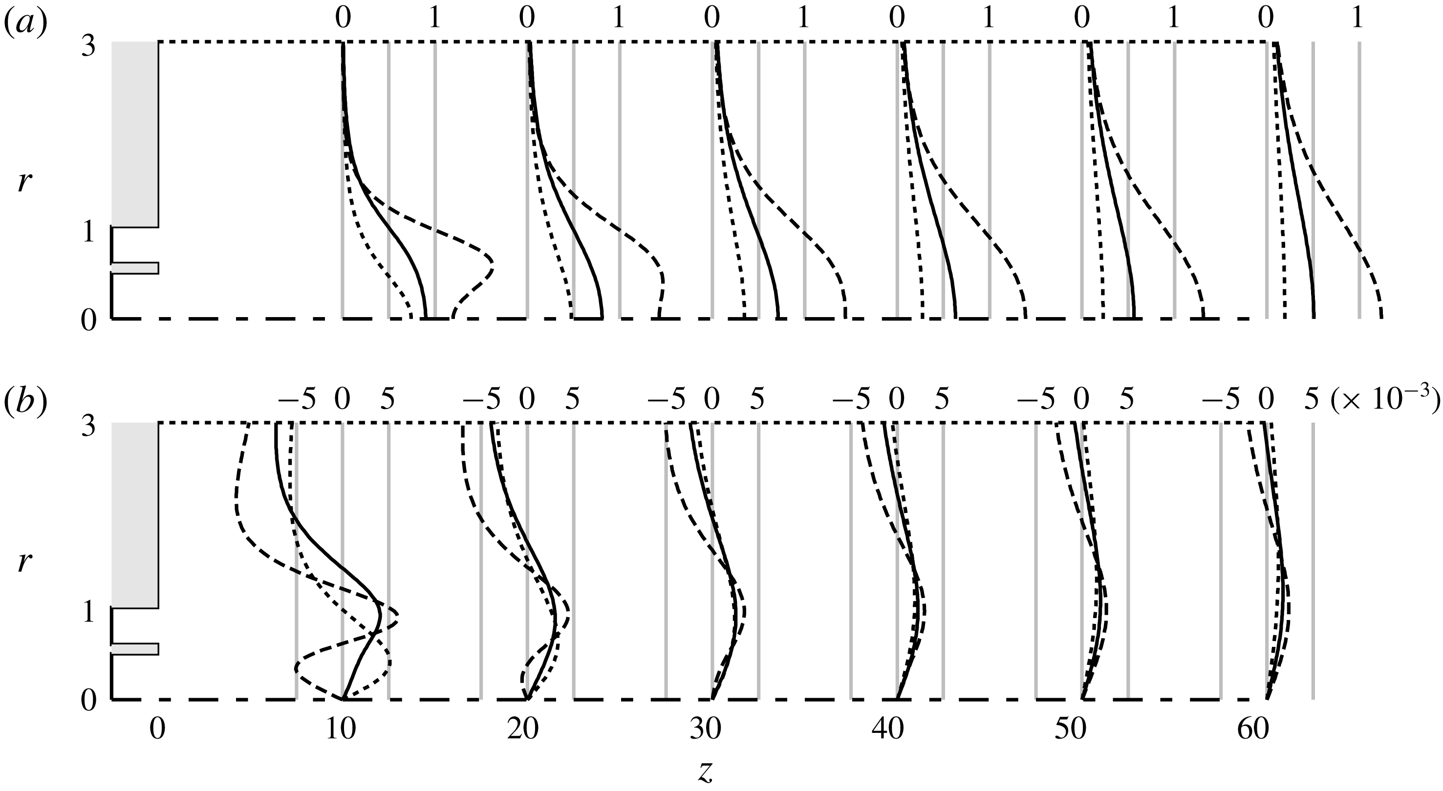
Influence of the velocity ratio
 $r_{u}$
on the (a) axial and (b) radial-velocity fields in the domain. Non-swirling jet for
 $Re=200$
,
 $r_{u}=0.0$
(dotted line),
 $r_{u}=1.0$
(solid line) and
 $r_{u}=2.0$
(dashed line).

The velocity profiles of the non-swirling jets are depicted in figure 3 for several distances from the orifice and for different values of the velocity ratio
 $r_{u}$
. In these non-swirling cases, the azimuthal component of the velocity is zero for symmetry. No recirculation bubble has been observed downstream of the septum separating the inlet ducts, for the values of the parameters under investigation. For velocity ratios lower than
 $r_{u}=1.0$
, the maximum axial velocity is attained on the axis and no other local maxima associated with the outer stream are observed for
 $z\geqslant 10$
. In this case, a single shear layer characterises the flow field in the region far from the nozzle, while three different shear layers are always present near the nozzle owing to the presence of the blunt wall separating the inner and outer jet. For
 $r_{u}=2.0$
, a local maximum is attained in the domain for
 $z\geqslant 10$
and a local minimum is observed on the axis for
 $z\leqslant 20$
. This behaviour of the axial velocity for high velocity ratios is associated with a non-trivial radial velocity profile, as shown in figure 3(b). For low velocity ratios, the positive values of
 $U_{r}$
near the axis and the negative values far from the axis are associated with the spreading of the jet core and the entrainment process, see Table 1, respectively. For
 $r_{u}=2.0$
, as the maximum of the axial velocity moves from the outer stream towards the axis for
 $z<20$
, a negative radial velocity is observed near the axis. Such a negative radial velocity is related, by incompressibility, to the transfer of momentum from the high-speed region of the jet to the near axis region, and in fact is no longer observed when the maximum of the axial velocity eventually reaches the axis.
Entrainment in stable non-swirling base flows. Ratio of the mass flow
 $Q(z)=2\unicode[STIX]{x03C0}\int _{r=0}^{R=3}U_{z}(r,z)r\,\text{d}r$
through circular surfaces orthogonal to the axis, and the mass flow at the inflow,
 $Q_{in}=Q_{in,i}+r_{u}Q_{in,o}=0.593+1.732~r_{u}$
.
 $Re=200$
.

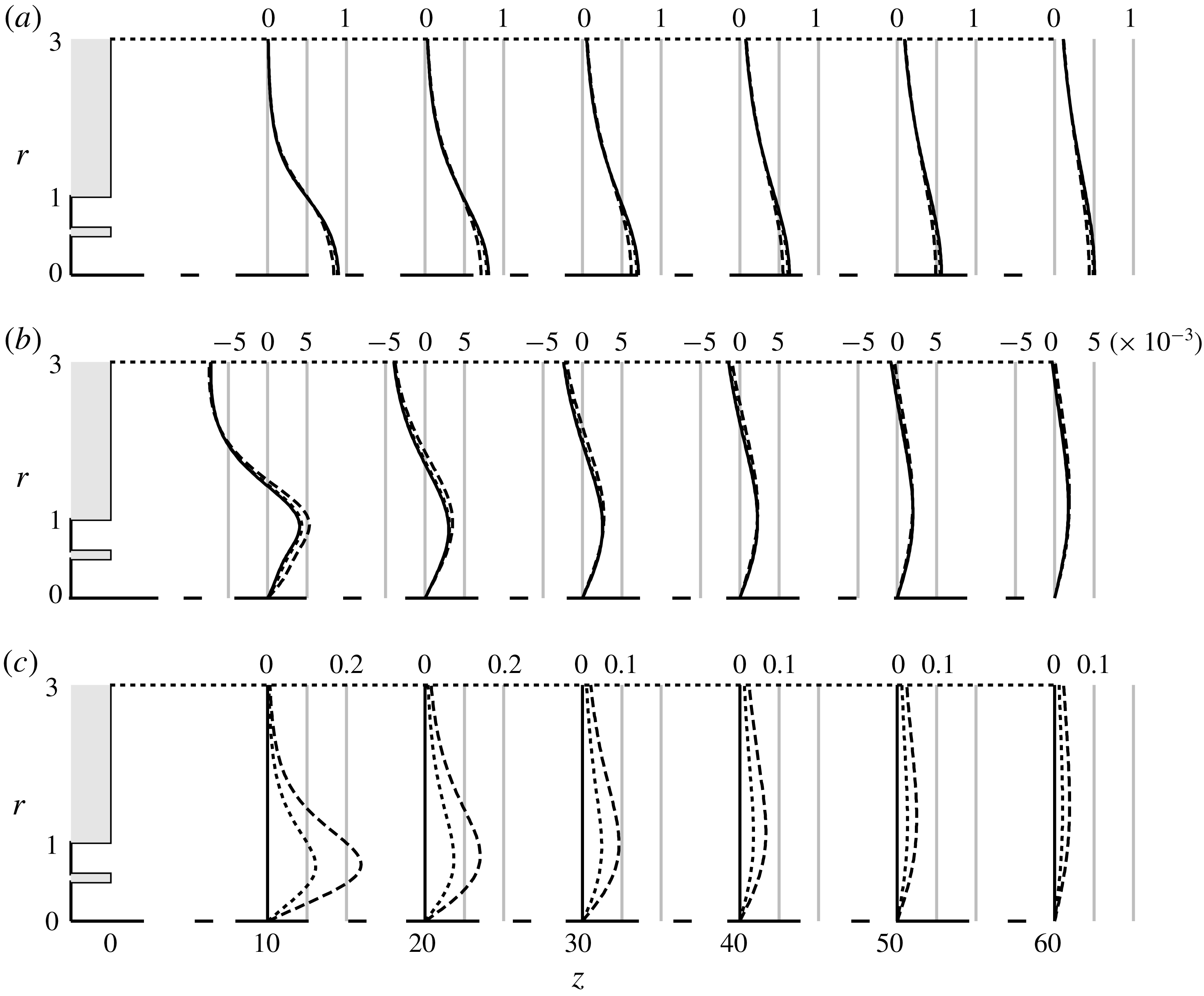
The velocity field is depicted in figure 4 for jets with unitary velocity ratio and different values of the swirl parameter. As is clear from the figure, the longitudinal and radial-velocity components of the base flow are quite insensitive to the swirl, for small swirl ratios. Despite this fact, as it will be appreciated later on, this parameter can impact the response of the flow to inflow perturbations quite dramatically.
5 Harmonic response
Despite this flow is absolutely stable, according to a global modal stability analysis (Canton et al.
Reference Canton, Auteri and Carini2017), transition to turbulence in jets has been observed for Reynolds numbers well below
 $Re=500$
(Reynolds Reference Reynolds1962). In fact, modal stability does not tell us the whole story, since non-normal systems, such as jets, may exhibit transient growth and pseudo-resonance (Reddy & Henningson Reference Reddy and Henningson1993; Schmid Reference Schmid2007), i.e. a large amplification of initial perturbations and external forcing in a restricted range of frequencies due to non-modal growth mechanisms. Such an amplification of perturbations, that are always present to a certain degree in an experiment, may lead to secondary instabilities and eventually to turbulence (Blackburn, Barkley & Sherwin Reference Blackburn, Barkley and Sherwin2008a
; Blackburn, Sherwin & Barkley Reference Blackburn, Sherwin and Barkley2008b
; Cantwell, Barkley & Blackburn Reference Cantwell, Barkley and Blackburn2010). The transient growth of axisymmetric perturbations has already been analysed by Canton et al. (Reference Canton, Auteri and Carini2017), who found huge amplification factors for a subcritical Reynolds number of
 $1000$
, while the harmonic response has been investigated for the single jet by Garnaud et al. (Reference Garnaud, Lesshafft, Schmid and Huerre2013b
) for the same Reynolds number. In this section, the harmonic response of the coaxial-jet flow to small-amplitude inflow forcing is investigated to explain the preferred dynamics of the system observed experimentally (Dahm et al.
Reference Dahm, Frieler and Tryggvason1992) or by direct numerical simulations with forcing applied at the inlet (Balarac et al.
Reference Balarac, Métais and Lesieur2007). The nonlinear response of the flow to inflow forcing is also investigated in § 6 by direct numerical simulation to investigate the relevance of the linear response when nonlinearities are present. A Reynolds number lower than that employed in the works by Garnaud et al. (Reference Garnaud, Lesshafft, Schmid and Huerre2013b
) and Canton et al. (Reference Canton, Auteri and Carini2017) has been preferred here to avoid the huge amplifications observed for Reynolds numbers of the order of
 $1000$
and therefore to better appreciate the spatial evolution of perturbations.
Influence of the swirl ratio
 $S$
of the outer stream on the (a) axial, (b) radial and (c) azimuthal velocity fields in the domain. Swirling jet for
 $Re=200$
and
 $r_{u}=1.0$
:
 $S=0.0$
(solid line),
 $S=0.5$
(dotted line) and
 $S=1.0$
(dashed line).

Influence of the velocity ratio
 $r_{u}$
on the harmonic response of non-swirling jets for
 $Re=200$
. Relative contributions of the wavenumbers in the harmonic response (a–c) and real part of the axial velocity
 $\hat{u} _{z}$
of the preferred response (d–f):
 $r_{u}=0.0$
(a,d);
 $r_{u}=0.5$
(b,e);
 $r_{u}=1.0$
(c,f). Thick lines in the left plots represent optimal gains, while thin lines represent the first suboptimal gain.

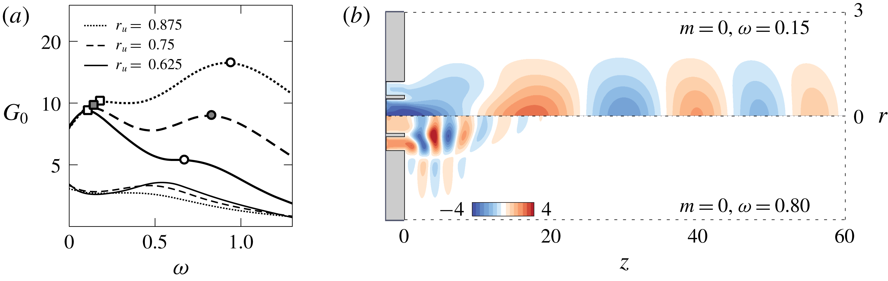
Influence of the velocity ratio
 $r_{u}\in (0.625,0.875)$
on the axisymmetric harmonic response of non-swirling jets for
 $Re=200$
. (a) Amplification
 $G_{0}$
of the optimal (thick lines) and first suboptimal (thin lines) axisymmetric harmonic response. Square and circle markers identify the first and the second local maximum, respectively, as in figure 7. (b) Real part of the axial velocity
 $\hat{u} _{z}$
of the two preferred axisymmetric responses for
 $r_{u}=0.75$
.

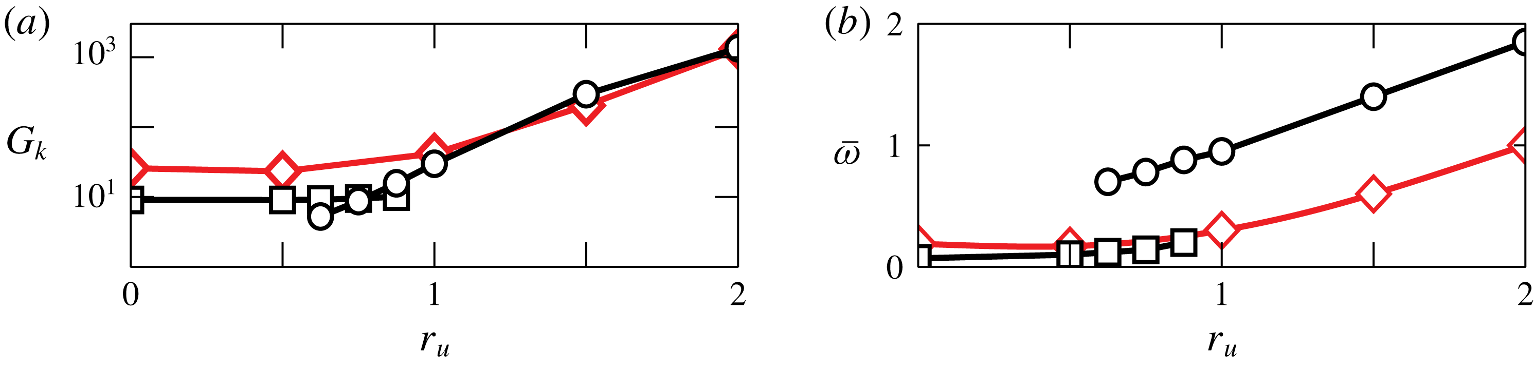
Influence of the velocity ratio
 $r_{u}$
on the harmonic response of non-swirling jets for
 $Re=200$
. (a) Amplification
 $G_{k}$
and (b) frequency
 $\overline{\unicode[STIX]{x1D714}}$
of the pseudo-resonance peaks. Line colours identify the wavenumbers:
 $m=0$
, black lines;
 $m=1$
, red lines with diamonds. Markers identify the preferred responses: squares and circles represent the first and the second peak of the axisymmetric harmonic gain, respectively.

5.1 Non-swirling jet
Firstly, the effect of the velocity ratio
 $r_{u}$
on the harmonic response of non-swirling jets with
 $Re=200$
is investigated. The relative contributions
 $g_{k}(\unicode[STIX]{x1D714})=G_{k}(\unicode[STIX]{x1D714})/\max _{i,\unicode[STIX]{x1D714}}\{G_{i}(\unicode[STIX]{x1D714})\}$
of the optimal and suboptimal responses associated with different wavenumbers are represented in figure 5(a–c) as functions of the frequency of the harmonic perturbations, for different values of the velocity ratio
 $r_{u}$
. The shape of the optimal responses is depicted in figure 5(d–f). The optimal sinuous and varicose responses, with azimuthal wavenumbers
 $m=+1$
and
 $m=0$
, respectively, prevail over the response to forcing with larger wavenumbers, so that results are reported in figure 7 only for these two wavenumbers. For instance, the harmonic gain of the optimal sinuous response of the single jet is approximately three times larger than the optimal axisymmetric gain. Dominant perturbations with
 $m=0$
and
 $m=+1$
were found also by Mattingly & Chang (Reference Mattingly and Chang1974), by an inviscid local linear stability analysis of the round jet, but in that case the
 $m=0$
perturbation was found to be more amplified. This result is similar to what has been found for the single jet by Morris (Reference Morris1976), see also Danaila, Dus̆ek & Anselmet (Reference Danaila, Dus̆ek and Anselmet1997). The varicose and sinuous modes emerge as dominant for different velocity ratios also in coaxial jets. It is interesting to note that Wicker & Eaton (Reference Wicker and Eaton1994) found that varicose and sinuous large-scale coherent structures are still dominating the flow behaviour at Reynolds numbers orders of magnitude higher. For low values of the velocity ratio, a local maximum appears on the axisymmetric optimal response, while both the frequency and the shape of the preferred axisymmetric response undergo substantial changes in the range of velocity ratio
 $r_{u}\in (0.5,\,1.0)$
, as shown in figure 5(b,c,e,f). A second local maximum appears in the optimal harmonic response at
 $\unicode[STIX]{x1D714}=0.67$
, it becomes the global maximum as the velocity ratio exceeds
 $r_{u}=0.75$
, while the low-frequency maximum progressively disappears for larger values of
 $r_{u}$
, see figure 6.
The optimal harmonic gain and the frequency of the pseudo-resonance peaks for
 $m=0$
and
 $m=+1$
are shown in figures 7(a) and 7(b), respectively, as functions of the velocity ratio
 $r_{u}$
. Two different regions can be distinguished in the two plots. For small velocity ratios,
 $r_{u}\lesssim 0.5$
, the maximum harmonic gain and its frequency are almost insensitive to
 $r_{u}$
. We conjecture that in this case the flow behaviour is dominated by the inner jet as in Segalini & Talamelli (Reference Segalini and Talamelli2011), or more precisely by the shear layer between the inner and outer jet that is rapidly amalgamated with the external shear layer, as visible in figure 2(a). This observation is confirmed by noticing that the shapes of the optimal responses for
 $r_{u}=0$
, namely for the single jet, and for
 $r_{u}=0.5$
, reported in figure 5(d,e), are very similar and that the optimal response reaches its maximum near the axis for
 $m=0$
and in a region that corresponds to the inner shear layer for
 $m=\pm 1$
. For higher velocity ratios,
 $r_{u}\gtrsim 1$
, the flow behaviour changes. The optimal responses for
 $m=0$
and
 $m=+1$
have very similar gain. The maximum amplification grows exponentially with the velocity ratio. This is especially evident for
 $m=\pm 1$
, while for
 $m=0$
there could be some saturation for
 $r_{u}>2$
, figure 7(a). More than one order of magnitude in the peak response amplitude is gained by just doubling the velocity ratio. This result is probably related to the exponential growth of the maximum harmonic gain as a function of the Reynolds number observed by Boujo & Gallaire (Reference Boujo and Gallaire2015) for the backward facing step, and that of the maximum transient growth observed by Cantwell et al. (Reference Cantwell, Barkley and Blackburn2010) for several wall-bounded separated flows. Indeed, in the present case the Reynolds number of the flow is computed as a function of the maximum velocity of the internal jet, but clearly the ratio of inertia terms over viscous terms for the external shear layer grows almost linearly with the velocity ratio
 $r_{u}$
when the Reynolds number is fixed. The frequency of the maximum amplification, the pseudo-resonance peak, grows linearly as a function of
 $r_{u}$
, figure 7(b), showing that, for sufficiently high velocity ratios, the flow properties scale with the external velocity and the outer jet dominates the stability properties of the flow (Rehab et al.
Reference Rehab, Villermaux and Hopfinger1997). It must be added here that the two preferred dynamics associated with the pseudo-resonance peaks in the harmonic response of the flow at
 $r_{u}=1.0$
persist for higher values of the velocity ratio. The trend observed here, with the ratio of the amplitudes of the axisymmetric and
 $m=\pm 1$
modes growing with the velocity ratio, has been observed also by Dahm et al. (Reference Dahm, Frieler and Tryggvason1992). Indeed, they reported the development of a sinuous
 $m=\pm 1$
mode for
 $r_{u}=0.59$
while an axisymmetric mode is observed for the higher
 $r_{u}=0.71$
, both associated with the external shear layer. Interestingly enough, our results show, see figure 7(a), a change in the dominating axisymmetric mode for
 $r_{u}=0.75$
. While the total amplification of the axisymmetric mode reaches that of the sinuous mode only for
 $r_{u}$
higher than
 $1$
, the former is more amplified near the nozzle than the latter, and could be therefore observed experimentally, especially for Reynolds numbers higher than the present ones.
The behaviour observed for the frequency of the optimal response is only partially coherent with the results reported by Segalini & Talamelli (Reference Segalini and Talamelli2011) that found three different behaviours as a function of the velocity ratio: for
 $r_{u}<0.75$
the frequency of the main peak in the radial-velocity spectrum scales as the velocity of the internal jet; for
 $r_{u}>1.6$
the frequency scales as the velocity of the external jet. These observations are coherent with the present results. For
 $0.75<r_{u}<1.6$
, however, Segalini & Talamelli (Reference Segalini and Talamelli2011) observed that the frequency depends on a combination of both. This behaviour is observed here for
 $m=\pm 1$
. For
 $m=0$
, the picture is more involved since, as previously observed, two different peaks in the optimal response exchange the role of pseudo-resonance in the interval
 $0.5<r_{u}<1$
. For
 $r_{u}<0.75$
, the frequency of the pseudo-resonance peak for
 $m=0$
scales as that of the optimal
 $m=\pm 1$
mode, consistently with Segalini & Talamelli (Reference Segalini and Talamelli2011). For
 $r_{u}\geqslant 0.75$
, the pseudo-resonance peak moves to a higher frequency, and its frequency scales almost as the external velocity, especially for
 $r_{u}\geqslant 1$
, as shown in figure 7(b). The radical change in the shape of the optimal response as
 $r_{u}$
is increased beyond
 $0.75$
is associated with the high-frequency dynamics that becomes dominant in this range of the parameter, as shown in figure 6(b). For low velocity ratios, figure 5(d,e), the optimal response is very elongated in the axial direction, with large structures that are more intense on the axis and slowly decay with
 $z$
. The axisymmetric structures for both
 $r_{u}=0$
and
 $r_{u}=0.5$
are similar to that found by Garnaud et al. (Reference Garnaud, Lesshafft, Schmid and Huerre2013b
) for the single jet, while the frequencies differ, probably due to the different Reynolds numbers. They presented the spatial structure of the response only for axisymmetric perturbations, so that a comparison is not possible for
 $m=1$
, but it must be said that they also observed a larger response for
 $m=1$
than for
 $m=0$
. For
 $r_{u}=1$
, we observe a totally different shape of the response. Firstly, the response has a frequency approximately one order of magnitude higher. Moreover, the space distribution of the response has two local maxima: one in the region of the external shear layer and one along a line starting from the wall separating the two jets and reaching the axis after more than ten internal diameters. The response spreads more in the radial direction than for lower velocity ratios. Finally, it is evident that the linear response decays very quickly, being almost negligible
 $20$
diameters downstream the jet exit. This behaviour is similar to what found experimentally by Dahm et al. (Reference Dahm, Frieler and Tryggvason1992) for
 $r_{u}=1$
and
 $1.14$
. They observed a wake-like instability in the shear layers produced by the separating wall frequency locked to the axisymmetric roll-up associated with the external shear layer. The shape of the axisymmetric mode in figure 5(f) seems to represent reasonably well both the instabilities. The change of shape is associated with the higher-frequency local maximum in the frequency response becoming dominant over the lower-frequency pseudo-resonance peak for
 $r_{u}\approx 0.75$
, as shown in figure 6(b). The shape of the response is very similar to that reported by Garnaud et al. (Reference Garnaud, Lesshafft, Schmid and Huerre2013b
) for the single jet, even if a local maximum is also found in the present case in the wake of the separating wall. In order to compare the Strouhal numbers, we need to take into account that, for
 $r_{u}=1$
, the jet behaves almost as a single jet with nozzle diameter equal to that of the external nozzle of the coaxial jets, and that the Reynolds numbers are different. The present result
 $\unicode[STIX]{x1D714}=1$
leads to a Strouhal number based on the diameter of the outer jet and on the maximum velocity of
 $0.31$
. This value, once rescaled for
 $Re=1000$
using a linear variation of the frequency with the Reynolds number obtained from results reported later on, agrees very well with the value
 $St=0.48$
reported by Garnaud et al. (Reference Garnaud, Lesshafft, Schmid and Huerre2013b
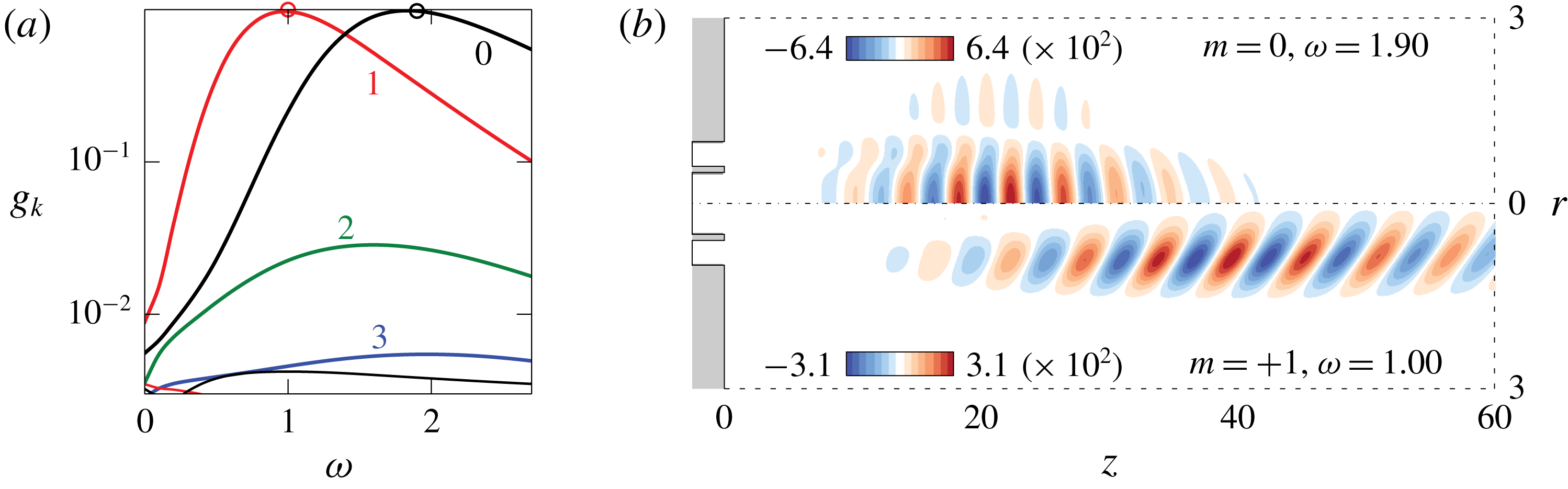
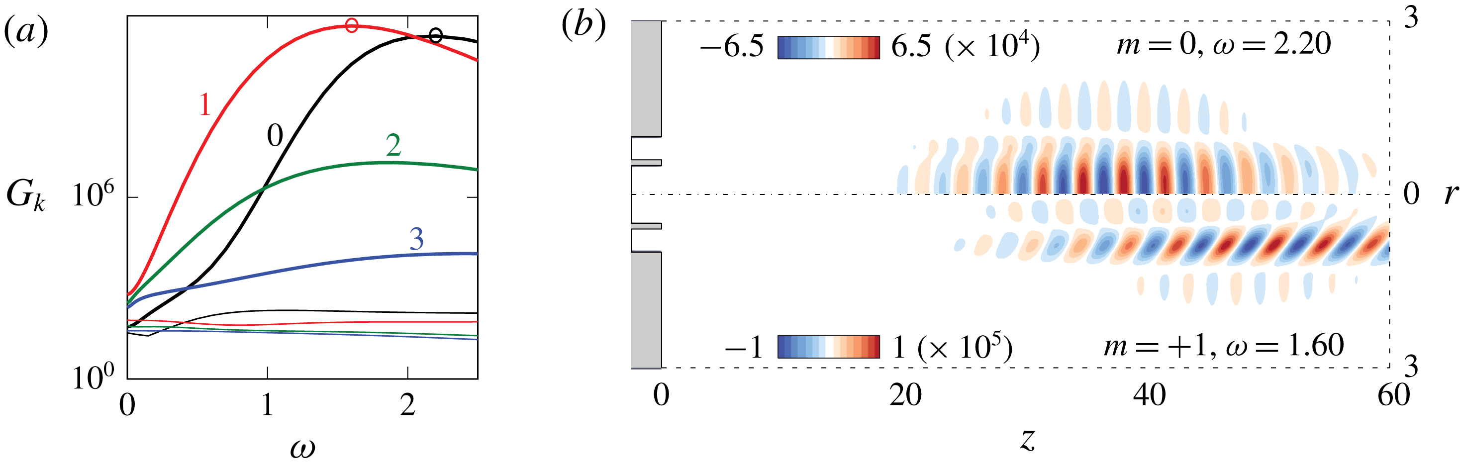
). The observed trend of the response as a function of the velocity ratio is confirmed by the results reported in figure 8 for a velocity ratio
 $r_{u}=2$
. The shape of the optimal response suggests that the flow is dominated by the outer shear layer for high velocity ratios. In this case, the amplification of the axisymmetric mode reaches the value of the sinuous mode with
 $m=\pm 1$
. The shape of the strongest response modes is very similar to that observed for
 $r_{u}=1$
, but the maximum of the optimal axisymmetric response moves considerably downstream. The fact that the axisymmetric response dominates in the region near the nozzle agrees with the experimental observations by Rehab et al. (Reference Rehab, Villermaux and Hopfinger1997) for non-rotating coaxial jets with
 $r_{u}\geqslant 2$
. It is interesting to note that the switch between the low
 $r_{u}$
behaviour and the high
 $r_{u}$
behaviour is observed for a velocity ratio for which the momentum flux exiting from the inner nozzle approximately equals that exiting from the outer nozzle.
Harmonic response for
 $(Re,r_{u},S)=(200,2.0,0)$
. (a) Relative contributions of the wavenumbers. Thick lines indicate the optimal harmonic gain, while thin lines the first suboptimal harmonic gain. The small circles on the curves correspond to the preferred response shown in panel (b). (b) Real part of the axial velocity
 $\hat{u} _{z}$
of the preferred response.

5.2 Effect of swirl
The effect of the swirl parameter is assessed for coaxial jets with
 $r_{u}=1$
. The rotation of the outer stream breaks the symmetry of the azimuthal coordinate
 $\unicode[STIX]{x1D703}$
, so that retrograde structures have positive wavenumbers in the series expansion (3.2) for positive values of
 $\unicode[STIX]{x1D714}$
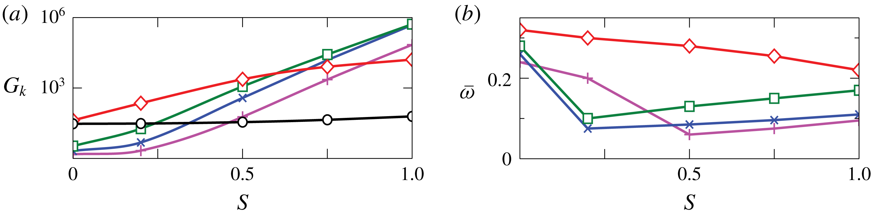
. While the amplification of axisymmetric structures remains almost unchanged, huge amplifications of the non-axisymmetric retrograde modes occur in swirling jets, see figure 9(a): the
 $m=+1$
mode prevails for low swirl, while the contribution of larger wavenumbers emerges as the swirl parameter
 $S$
exceeds
 $0.6$
, see figure 10(a,b). The optimal amplification of structures with wavenumbers
 $2$
,
 $3$
,
 $4$
grows exponentially fast for
 $S>0.5$
. The response of the system associated with negative azimuthal wavenumbers corresponding to forward rotation rapidly decays with
 $\unicode[STIX]{x1D714}$
and
 $S$
, see dotted lines in figure 10(a,c). For
 $S=1$
, the retrograde structures with wavenumbers
 $+2$
and
 $+3$
are dominant (c).
Influence of the swirl parameter
 $S$
on the harmonic response: coaxial jets with unitary velocity ratio and
 $Re=200$
. (a) Optimal amplification
 $G_{k}$
and (b) frequency
 $\overline{\unicode[STIX]{x1D714}}$
of the pseudo-resonance peak. Line colours and markers identify the wavenumbers:
 $m=0$
black circles;
 $m=+1$
red diamonds;
 $m=+2$
green squares;
 $m=+3$
blue crosses;
 $m=+4$
magenta plus markers. The pseudo-resonance peak of the axisymmetric mode is approximately
 $\overline{\unicode[STIX]{x1D714}}_{0}\approx 1$
over the whole range of
 $S$
explored. Only retrograde dynamics is represented.

Influence of the swirl parameter
 $S$
on the harmonic response of coaxial jets with unitary axial velocity ratio
 $r_{u}=1$
and
 $Re=200$
. Relative contributions of the wavenumbers in the harmonic response (a–c) and real part of the axial velocity
 $\hat{u} _{z}$
of the preferred response (d–f):
 $S=0.2$
(a,d);
 $S=0.5$
(b,e);
 $S=1.0$
(c,f). Solid lines: counter-winding structures with
 $m\geqslant 0$
; dotted lines: co-winding structures with
 $m<0$
.

The analysis of the spatial structure of the optimal response is also interesting. For
 $S=0.2$
, figure 10(d), the optimal response, a single retrograde helix with wavenumber
 $m=+1$
, is mostly amplified quite far from the nozzle. The maximum of the response is observed for a radius slightly less than one. On this point, it is interesting to observe that Leibovich & Stewartson (Reference Leibovich and Stewartson1983) predicted that the eigenfunctions should be maximum around
 $R=1$
, and this property was observed also for the peak of the impulse response of a swirling jet by Gallaire & Chomaz (Reference Gallaire and Chomaz2003b
). As the swirl number is increased, figure 10(b,c), the optimal response is associated with increasing wavenumbers, but the spatial structure of the optimal response does not change dramatically. The maximum of the response moves farther from the nozzle as the swirl number is increased; the opposite trend is observed as the wavenumber is increased. The optimal response associated with these helical structures extends throughout the whole domain. Moreover, it can be observed that the radius where the maximum of the optimal response is observed slowly grows with the swirl number, while remaining always in the neighbourhood of
 $r=1$
. This effect is probably related to the slow growth of the radius of the jet as the swirl number is increased, see figure 4(a).
Despite the difference in the base flow and Reynolds number, our results seem to qualitatively agree with the experimental results reported by Liang & Maxworthy (Reference Liang and Maxworthy2005). Indeed, for strongly swirling jets before vortex breakdown, they found an instability in the form of retrograde, i.e. counter-winding, helical waves with
 $m=+2$
and
 $m=+3$
. For smaller values of the swirl number, the instability is associated with axisymmetric annular vortices, while spiral vortices are associated with a secondary instability. This last observation is not completely in contrast with our results. While for small swirl the axisymmetric mode is globally less amplified than the
 $m=+1$
helical mode, it is indeed stronger in the region near the nozzle. Therefore, we conjecture that we observe axisymmetric vortices since they are the most amplified ones near the nozzle. Then, a secondary instability sets in before the helical mode is sufficiently amplified to be visible, as will be clearer in the next section. In contrast, our result is different from that reported by Gallaire & Chomaz (Reference Gallaire and Chomaz2003b
) where co-winding modes are most amplified. The main reason to explain this discrepancy probably relies in the different base flow. In the present case, since only the outer jet is swirling, two azimuthal shear layers are present that are at the origin of the observed counter-winding modes. As a confirmation, we observe that Weller-Calvo, Joly & Fontane (Reference Weller-Calvo, Joly and Fontane2013) did not find such modes by a linear stability analysis of the parallel coaxial-jet flow for
 $r_{u}\approx 1$
, when only the central jet is swirling.
5.3 Effect of the Reynolds number
The influence of the Reynolds number
 $Re$
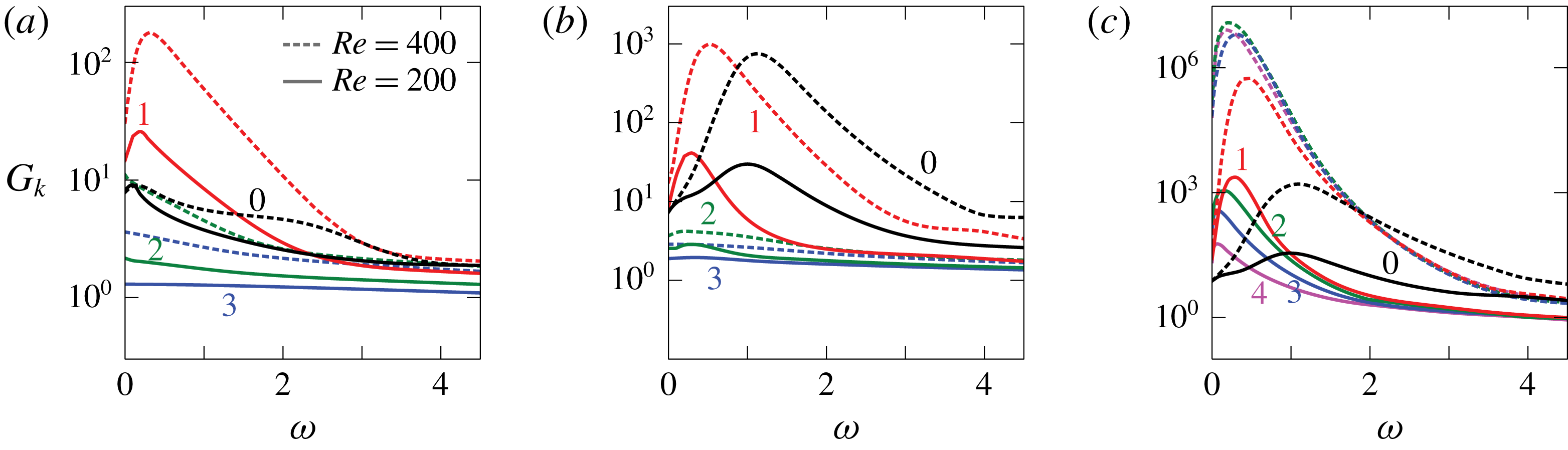
on three flow configurations is summarised in figure 11. In general, we can say that the Reynolds number mainly affects the magnitude of the amplification while it has only a minor impact on the frequency of the pseudo-resonance peaks. For the single jet, figure 11(a), two main effects are observed. The amplitudes of sinuous response modes with
 $m=+1$
,
 $m=+2$
and
 $m=+3$
increase significantly with the Reynolds number. The most amplified response corresponds to
 $m=\pm 1$
. The peak response amplitude of the axisymmetric mode, in contrast, does not change significantly, but a second local maximum appears for a non-dimensional circular frequency
 $\unicode[STIX]{x1D714}\approx 2$
. The situation is different when a coaxial jet with unitary velocity ratio is concerned, figure 11(b). In this case, all the responses with lower wavenumber
 $m=0\div 3$
increase significantly. In particular, for the
 $m=0$
and
 $m=+1$
modes the amplitude increases by more than an order of magnitude. For the axisymmetric mode the increase seems a bit larger. This fact may in part explain why, for higher Reynolds numbers, the axisymmetric mode dominates the flow dynamics near the nozzle (Dahm et al.
Reference Dahm, Frieler and Tryggvason1992). This behaviour is slightly different when a velocity ratio
 $r_{u}=2$
is considered, figure 12(a) to be compared with figure 8(a), with a slightly stronger increase in the amplitude of the response of the azimuthal wavenumbers
 $m=\pm 1$
,
 $\pm 2$
and
 $\pm 3$
with respect to the axisymmetric perturbations. When a swirl is present, the picture changes dramatically. From figure 11(c) it is apparent that the responses of perturbations with higher wavenumbers,
 $m=+2,\,+3,\,+4$
, increase most with the Reynolds number, so that they become dominant over the response for
 $m=+1$
. The increase in the amplitude is also notable: more than three orders of magnitude by just doubling the Reynolds numbers. The amplification of the most amplified modes is very similar, so that it is hard to predict which wavenumber will be selected in the actual flow. A nonlinear analysis as in Mantic̆-Lugo & Gallaire (Reference Mantic̆-Lugo and Gallaire2016) seems to be necessary to answer this question, but it is out of the scope of the present work.
Influence of the Reynolds number
 $Re$
on the harmonic response of three configurations of the system: (a) single jet; (b) non-swirling coaxial jets with unitary velocity ratio; (c) coaxial jets with unitary velocity ratio and swirl parameter
 $S=0.5$
. Solid lines:
 $Re=200$
; dotted lines:
 $Re=400$
. Colours as in the caption of figure 9.

Harmonic response for
 $(Re,r_{u},S)=(400,2.0,0)$
. (a) Relative contributions of the wavenumbers. Thick lines indicate the optimal harmonic gain, while thin lines the first suboptimal harmonic gain. The small circles on the curves correspond to the preferred response shown in panel (b). (b) Real part of the axial velocity
 $\hat{u} _{z}$
of the preferred response.

It is also interesting to compare the change induced by an increase in the Reynolds number in the shape of the optimal response. This is possible by looking at figures 12(b) and 8(b). From the figures, it is apparent that increasing the Reynolds number moves the maximum of the amplitude farther from the nozzle. For
 $m=\pm 1$
there is also a change in the shape of the response. The maximum response concentrates in the outer jet, with non-negligible contributions coming from the inner jet and from the outer region.
6 Nonlinear simulations
The validity of the assumptions made, the results of the harmonic response and the predominance of the harmonic response of the perturbed system are assessed by means of three-dimensional, nonlinear time simulations. All the flows analysed in this chapter are globally stable but behave as noise amplifiers: no self-sustained oscillations are observed in the system with nominal boundary conditions, namely a flow supplied with the steady boundary conditions that were used to compute the base flow, see § 2. The situation may change dramatically when perturbations are present. As a matter of fact, the strong amplification of the disturbances at the inflow, that inevitably characterise experiments, may result in substantial deviation of the flow from its stable base state. Therefore, a random disturbance, uncorrelated in both time and space and among the velocity components, has been added to the nominal boundary conditions. The disturbance has a maximum amplitude of
 $2.5\,\%$
of the reference velocity and it is uniformly distributed in the interval
 $(-0.025\widetilde{U}_{a},0.025\widetilde{U}_{a})$
. While the assumption that disturbances can be well represented by a band-limited white noise may seem crude, two observations are in order: the actual noise in an experiment or in a real device can hardly be fully characterised, especially when complex nozzle geometries are concerned as in swirled burners. Vorticity in the wake of internal obstacles, acoustic and thermal perturbations and incoming turbulence can all be causes of inlet perturbations. Moreover, the stochastic response analysis relying on the harmonic response analysis usually assumes a white noise as input. As a matter of fact, it is generally recognised that a white noise can be considered a sufficiently general and accurate approximation to investigate the jet behaviour in an experimental environment (Cohen & Wygnanski Reference Cohen and Wygnanski1987; Balarac et al.
Reference Balarac, Métais and Lesieur2007; Gohil, Saha & Muralidhar Reference Gohil, Saha and Muralidhar2012; Jeun, Nichols & Jovanovi Reference Jeun, Nichols and Jovanovi2016). This assumption is also exploited in recent works on the prediction of large coherent structures, which characterise the early development of turbulent jets, carried out by a resolvent analysis similar to the present one applied to the mean flow, obtained either experimentally (Semeraro et al.
Reference Semeraro, Jaunet, Jordan, Cavalieri and Lesshafft2016; Lesshafft et al.
Reference Lesshafft, Semeraro, Jaunet, Cavalieri and Jordan2018) or numerically (Schmidt et al.
Reference Schmidt, Towne, Rigas, Colonius and Brès2018). The very good match between the coherent structures educted by linear resolvent analysis and those extracted from the experiments and nonlinear simulations testifies for the applicability of the assumption. The introduction of perturbations is meant to investigate the relevance of the results of the linear input–output analysis in predicting the nonlinear dynamics of real coaxial jets. The amplitude of the perturbations has been chosen sufficiently high to make the amplified perturbations significant in a sufficiently short distance from the nozzle for the low Reynolds numbers investigated here, even if, from the viewpoint of a laboratory experiment, they can be considered quite high. The adopted amplitude is actually slightly less than that used by Balarac et al. (Reference Balarac, Métais and Lesieur2007) in their direct numerical simulations (DNS) at
 $Re=3000$
.
6.1 Coaxial jets
 $(Re,r_{u},S)=(200,2.0,0)$

We begin with a non-swirled jet with velocity ratio
 $r_{u}=2$
. Starting the simulation from the globally stable base flow, the transient growth of quite a coherent structure is observed after the noise is turned on: an axisymmetric perturbation grows in the domain while it is convected downstream. When this initial perturbation is convected out of the domain and the initial transient is over, clear dynamics appears: axisymmetric oscillations, in the form of annular vortices, with a frequency
 $\unicode[STIX]{x1D714}\approx 2.0$
develop in the upstream part of the domain; these annular perturbations tilt and a sinuous structure arises in the second half of the domain, whose frequency is half of the original one.
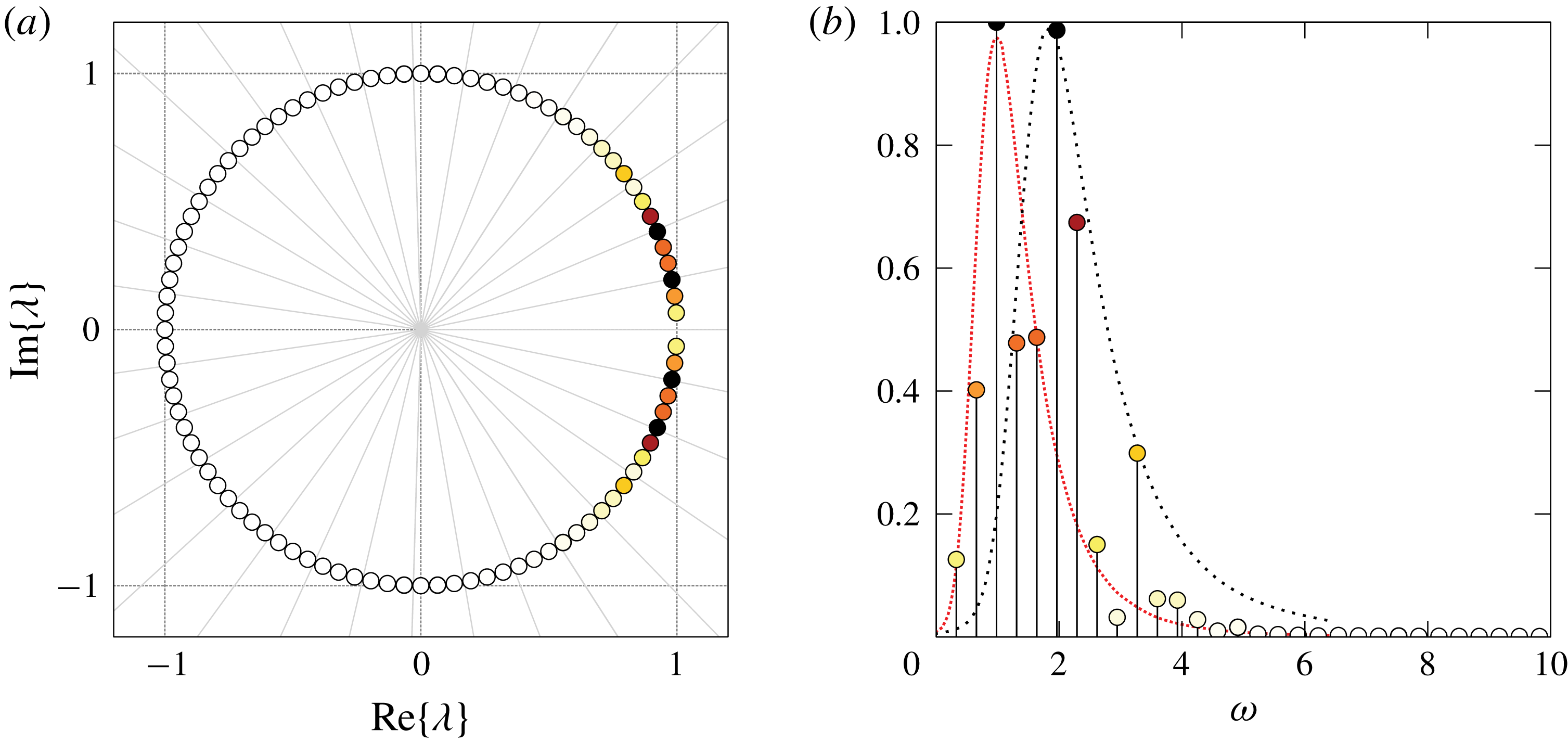
Koopman analysis of the flow for
 $(Re,r_{u},S)=(200,2.0,0)$
. (a) Koopman values
 $\unicode[STIX]{x1D706}_{j}$
in the complex plane: two consecutive light grey radii enclose a circular sector spanning
 $\unicode[STIX]{x0394}\unicode[STIX]{x1D714}=1.0$
. The marker colour varies from white to black according to the mode amplitudes, as defined in the right figure; (b) normalised amplitudes of the Koopman modes. Thin loosely and densely dotted lines represent the optimal harmonic gains of the axisymmetric and sinuous mode, respectively.

The Koopman mode analysis is used here to obtain a better insight into the dynamics of the perturbed jet. A sequence of
 $n=96$
snapshots
 $\unicode[STIX]{x1D61C}_{0}^{n}=\{\boldsymbol{u}_{i}\}_{i=0}^{n}=\{\boldsymbol{u}(t_{0}+\text{i}\unicode[STIX]{x0394}t)\}_{i=0}^{n}$
, sampled every
 $\unicode[STIX]{x0394}t=0.2$
time units, is used in the analysis to identify the structures associated with the two main frequencies. The corresponding sampling frequency is largely sufficient to capture all the amplified perturbations. Sampling starts at
 $t_{0}=200.0$
in order to exclude the transient behaviour. All the Koopman values lie on the unit circle in the complex plane, i.e.
 $|\unicode[STIX]{x1D706}_{j}|=1.0$
, indicating that the system evolves on an attracting set (Rowley et al.
Reference Rowley, Mezi, Bagheri, Schlatter and Henningson2009), see figure 13(a). The two prevailing modes oscillate with circular frequencies
 $\unicode[STIX]{x1D714}_{1}=\measuredangle \unicode[STIX]{x1D706}_{1}/\unicode[STIX]{x0394}t=0.98$
and
 $\unicode[STIX]{x1D714}_{2}=1.97$
: these values are very close to the pseudo-resonance peaks in the harmonic response of the sinuous mode
 $\hat{\boldsymbol{u}}_{1}(\unicode[STIX]{x1D714})$
with wavenumber
 $m=1$
and the axisymmetric mode
 $\hat{\boldsymbol{u}}_{0}(\unicode[STIX]{x1D714})$
. Only positive frequencies are shown in figure 13(b), since the Koopman values and modes come in complex-conjugate pairs. The first Koopman mode, oscillating at
 $\unicode[STIX]{x1D714}_{1}$
, is associated with the low-frequency sinuous structure arising in the downstream portion of the domain, see figure 14(a): this structure closely resembles the optimal harmonic response
 $\hat{\boldsymbol{u}}_{1}(1.0)$
close to the pseudo-resonant peak shown in figure 14(b). The second Koopman mode, oscillating at
 $\unicode[STIX]{x1D714}_{2}$
, is associated with the axisymmetric perturbations observed close to the nozzle whose contour levels are depicted in figure 15(a): the axisymmetric structure grows in the upstream part of the domain before starting to decay and lose its symmetry, and being eclipsed by the sinuous structure further downstream. This Koopman mode clearly resembles the axisymmetric preferred response
 $\hat{\boldsymbol{u}}_{0}(2.0)$
in the upstream portion of the domain depicted in figure 15(b). These observations suggest that the evolution of these modes is almost independent of each other, for such a low Reynolds number and amplitude, with the linear receptivity of the flow being responsible for selecting, by linear amplification, the dominating dynamics in each region of the flow. Apparently, the nonlinear interaction between the two most amplified modes does not play a role, for the present value of the parameters. Therefore, the linear analysis is sufficient to draw a clear picture of the flow behaviour in this case. It is interesting to note that the spatial structure of the modes plays an important role, not only their amplification. Indeed, the axisymmetric mode is dominant upstream while the sinuous mode with
 $m=\pm 1$
is dominant downstream, exactly as anticipated by the linear input–output analysis.
Koopman mode 1 (sinuous) for the flow with
 $(Re,r_{u},S)=(200,2.0,0)$
. (a) Real part of the axial velocity: contour levels corresponding to 15 % (opaque) and 2 % (transparent) of the maximum value in the domain. (b) Contour lines of the axial velocity of the optimal harmonic response for
 $m=+1$
,
 $\unicode[STIX]{x1D714}=1.0$
superimposed on a slice of the first Koopman mode.

Koopman mode 2 (varicose) for the flow with
 $(Re,r_{u},S)=(200,2.0,0)$
. (a) Real part of the axial velocity: contour levels corresponding to 15 % (opaque) and 2 % (transparent) of the maximum value in the domain. (b) Contour lines of the axial velocity of the optimal harmonic response for
 $m=0$
,
 $\unicode[STIX]{x1D714}=2.0$
superimposed on a slice of the second Koopman mode.

Coaxial jets with
 $(Re,r_{u},S)=(400,2.0,0)$
. Dynamic-mode decomposition (DMD) analysis of nonlinear time simulations: spectra and prevalent Koopman modes. (a,b)
 $z_{\mathit{DMD}}=20$
, (c,d)
 $z_{\mathit{DMD}}=25$
, (e,f)
 $z_{\mathit{DMD}}=L_{c}=60$
.

6.2 Coaxial jets
$(Re,r_{u},S)=(400,2.0,0)$

As explained in § 5, the amplification of the incoming disturbances rapidly grows with the Reynolds number. It is therefore interesting to investigate the impact of an increased Reynolds number on the fate of inlet perturbations. For this purpose, we run a DNS for a non-swirling jet with
 $r_{u}=2$
as before, but with double the Reynolds number,
 $Re=400$
. The random perturbations have the same properties as in the previous case. While two coherent oscillating structures, that behave almost independently from each other, have been observed in the previous section for
 $Re=200$
, velocity perturbations at the inflow promote the transition to a turbulent regime in the globally stable flow for
 $Re=400$
, see figure 16. As happened for the lower Reynolds number, also in this case the varicose mode obtained by the optimal harmonic response prevails in the upstream part of the domain, for
 $z<20$
. This is expected, since the varicose mode dominates the linear response in the region closer to the nozzle. The varicose mode appears as a train of axisymmetric vortices that arise owing to a Kelvin–Helmholtz instability of the shear layers formed by the outer jet. After a few jet diameters from the nozzle, the vortices start interacting nonlinearly, rolling up and pairing, and are finally subject to a three-dimensional instability.
The Koopman analysis of the entire flow field highlights the prevalent low-frequency broadband dynamics of the turbulent region, as reported in figure 16(e,f). The spectrum is almost monotonically decaying with the frequency, figure 16(e), while the dominating Koopman modes reported in figure 16(f) show a highly irregular pattern and the linear spreading typical of the turbulent jet (Balarac & Métais Reference Balarac and Métais2005). Since, in the Koopman analysis, the dynamics in the turbulent region stands above the coherent oscillations of the jet close to the nozzle, the laminar and transitional flow in the initial part of the jet is examined by analysing the flow field on a truncated domain for
 $z<z_{\mathit{DMD}}$
. After a cutoff coordinate
 $z_{\mathit{DMD}}$
is chosen, the observable is defined as the restriction of the velocity field to the truncated domain. Two different truncated domains have been analysed, with different lengths:
 $z_{\mathit{DMD}}=20$
, that represent approximately the location where the amplitude of the response in the nonlinear simulation is small, and
 $z_{\mathit{DMD}}=25$
, that represents the approximate maximum axial coordinate for which an ordered flow is observed in the simulation. The comparison of figure 16(b,d,f) shows clearly that the amplitude of the Koopman modes grows with the length of the truncated domain, from this observation we infer that the amplitude of the response keeps growing until the flow becomes turbulent.
Let us consider the Koopman analysis carried out in the shortest domain, namely for
 $z_{\mathit{DMD}}=20$
. The frequency–amplitude plot reported in figure 16(a) clearly shows two peaks. One, has a frequency
 $\unicode[STIX]{x1D714}=2.4$
that matches quite closely the most amplified axisymmetric forcing at the inlet,
 $\unicode[STIX]{x1D714}_{0}=2.2$
. The second one has a frequency
 $\unicode[STIX]{x1D714}=3.9$
that does not correspond to any of the peaks of harmonic gain for the tested azimuthal wavenumbers
 $m$
. On this point, it is interesting to analyse the most amplified mode at the truncation threshold. In this case we have a circular frequency slightly larger than
 $2.2$
for the axisymmetric response, while
 $\unicode[STIX]{x1D714}_{\pm 1}\approx 2.2$
. It must be said that the amplification of the axisymmetric mode is approximately one order of magnitude larger than that of the sinuous mode for this abscissa. This is probably the reason why the sinuous mode, that can reach an amplification factor two orders of magnitude larger further downstream, does not dominate over the axisymmetric mode in the present results. The fact that axisymmetric perturbations are most amplified in this region explains the basically axisymmetric character of the dominant Koopman modes reported in figure 16(b). Actually, the higher-frequency peak observed in figure 16(a) corresponds to that of most amplified mode for a shorter truncation,
 $z_{\mathit{DMD}}=8$
, not shown here for conciseness. The persistence of such a peak for longer distances from the nozzle could be related to nonlinear selection effects.
For
 $z>20$
, the flow strongly departs from axial symmetry. A detailed analysis of the transition process is out of the scope of the present work, but we just observe that, as a result of the interaction of the oscillations in the high-velocity annular region, a predominant transitional mode emerges with
 $\unicode[STIX]{x1D714}=1.3$
, figure 16(c,d), significantly lower than that of the aforementioned dominant linear modes. This fact is not surprising, since the nonlinear vortex roll-up and pairing may lead to a significant decrease of the peak frequency in the spectrum.
A question arises about which, of the dominant modes observed for
 $z_{\mathit{DMD}}=20$
, dominates the transition process, since in the linear analysis there is no evidence of the dominance of one mode over another. To investigate this point, we ran simulations where we forced the jet with the optimal inlet forcing with
 $m=0$
and
 $m=+1$
resulting from the optimal harmonic-gain analysis described in the previous section, see figure 17. The simulations show that the dynamics of the jet forced with
 $m=0$
leads to transition by the process of vortex roll-up, vortex pairing and instability of the vorticity braid connecting two adjacent vortices that produces outward ejections and quickly leads to transition to turbulence, as described for the single jet in Brancher, Chomaz & Huerre (Reference Brancher, Chomaz and Huerre1994) and Liepmann & Gharib (Reference Liepmann and Gharib1992). A different process is observed when the jet is forced with
 $m=+1$
. In this case, a sinuous mode prevails similar to that observed in swirling jets and leads to vortex breakdown. The jet becomes turbulent just after the core of the jet shows a marked helical shape. By comparing the nonlinear response of two jets forced with the same amplitude, it can be observed that the transition process is significantly faster in the second case, namely when the jet is forced with
 $m=+1$
. While this observation does not answer to the previous question, it seems to indicate that for this value of the parameters, the effectiveness of the two forcing modes in producing transition to turbulence is not equivalent, with the
 $m=\pm 1$
inlet forcing, the most amplified according to the linear analysis, being more effective.
Nonlinear response of the coaxial jet to optimal forcing with wavenumber
 $m=0$
(a), and
 $m=1$
(b), for
 $(Re,r_{u},S)=(400,2.0,0)$
. The
 $Q$
criterion is used to visualise the vortical structures in three dimensions in both cases. The colour map corresponds to the axial-velocity component in a radial plane.

6.3 Swirling coaxial jets
$(Re,r_{u},S)=(200,1.0,1.0)$

We now investigate the impact of a swirling outer jet on the behaviour of the flow in the nonlinear regime. A DNS of the coaxial jets with unit axial velocity ratio
 $r_{u}=1.0$
and swirling outer stream with
 $S=1.0$
shows a non-trivial combination of structures with different azimuthal wavenumbers. This behaviour was somehow expected, since the amplitude of the linear response depicted in figure 10(c) shows that several modes with different wavenumbers enjoy a strong amplification, those with
 $m=+2$
and
 $m=+3$
being the most amplified ones.
To better understand the flow behaviour, we sliced the velocity field with a plane normal to the axial direction and analysed the velocity field in such a plane. The axial-velocity field on the slice
 $\unicode[STIX]{x1D6FA}_{\overline{z}}$
, with
 $\overline{z}=35.0$
unit lengths far from the nozzle, is shown in figure 18(a): the prevalence of a structure with azimuthal wavenumber
 $m=+3$
becomes evident in figure 18(b) where the velocity field is purged of the axisymmetric contribution. This behaviour can be interpreted by looking at figure 10(c,f). From figure 10(c), it is clear that the two modes with
 $m=+2$
and
 $m=+3$
are dominant, with the former slightly prevailing over the latter. Figure 10(f), however, shows that the mode
 $m=+3$
reaches its maximum for a distance from the nozzle lower than that of the mode
 $m=+2$
, so that it not surprising that its contribution dominates for
 $\overline{z}=35.0$
. This slice of the velocity field is analysed by Fourier series in the azimuthal coordinate
 $\unicode[STIX]{x1D703}$
,
 $$\begin{eqnarray}\boldsymbol{u}(r,\unicode[STIX]{x1D703},\overline{z},\overline{t})=\mathop{\sum }_{m=-\infty }^{\infty }\tilde{\boldsymbol{u}}_{m}(r,\overline{z},\overline{t})\text{e}^{\text{i}m\unicode[STIX]{x1D703}}=\mathop{\sum }_{m=0}^{\infty }\boldsymbol{u}_{m}(r,\unicode[STIX]{x1D703},\overline{z},\overline{t}),\end{eqnarray}$$
in order to obtain a more detailed information about the wavenumber contributions. It is worthwhile noting that the discretisation of the transverse slice into
 $N_{\unicode[STIX]{x1D703}}=60$
circular sectors implies that the series is truncated to
 $|m|\leqslant N_{\unicode[STIX]{x1D703}}/2$
. The real contribution
 $\boldsymbol{u}_{m}=2re\{\tilde{\boldsymbol{u}}_{m}\text{e}^{\text{i}m\unicode[STIX]{x1D703}}\}$
of the lower positive wavenumbers is depicted in figure 18(d–f): more than
 $97\,\%$
of the
 $L^{2}$
-norm of the non-axisymmetric part of the field comes from the first three modes, see figure 19(c), and the contribution of the fourth mode is approximately
 $1.7\,\%$
.
Coaxial jets for
 $(Re,r_{u},S)=(200,1.0,1.0)$
. Axial component
 $u_{z}(r,\unicode[STIX]{x1D703},\overline{z},\overline{t})$
of the velocity field on the transverse section
 $\overline{z}=35.0$
. (a) Field at time
 $\overline{t}=490.0$
; (b) non-axisymmetric part of the field,
 $u_{z}-u_{z,0}$
; (d–f) non-axisymmetric real modes
 $u_{z,1}$
,
 $u_{z,2}$
,
 $u_{z,3}$
, whose contribution
 $\sum _{k=1}^{3}u_{z,k}$
is shown in figure (c). The relative contribution of a mode to the complete field is defined as the ratio of
 $L^{2}$
-norms,
 $p_{m}=\Vert \boldsymbol{u}_{m}\Vert _{L^{2}(\unicode[STIX]{x1D6FA}_{\bar{z}})}/\Vert \boldsymbol{u}\Vert _{L^{2}(\unicode[STIX]{x1D6FA}_{\bar{z}})}$
. In contrast to what has been done in previous figures, black contours are used in this figure only to increase the readability of the colour map.

The time average of the
 $L^{2}$
-norm of the velocity field
 $$\begin{eqnarray}A_{m}={\displaystyle \frac{1}{T}}\int _{t_{i}}^{t_{i}+T}\Vert \boldsymbol{u}_{m}\Vert _{L^{2}(\unicode[STIX]{x1D6FA}_{z})},\end{eqnarray}$$
is used in figure 19(a–c) to evaluate the relative shares of the modes in three different sections of the domain. The initial time
 $t_{i}$
is set to
 $300$
in order to exclude the transient behaviour and
 $T$
is set to
 $300$
as well. While energy is almost evenly distributed among the first three modes at
 $z=15.0$
, the second and the third modes prevail downstream along the domain (b,c). Higher wavenumbers have little contributions only in terms of energy. Figure 19(d) shows the temporal evolution of the integral quantity
 $$\begin{eqnarray}I(\unicode[STIX]{x1D703},t)=\int _{0}^{R}|\boldsymbol{u}(r,\unicode[STIX]{x1D703},\overline{z},t)|r\,\text{d}r.\end{eqnarray}$$
Coaxial jets for
 $(Re,r_{u},S)=(200,1.0,1.0)$
. Time-averaged mode contributions as functions of the axial coordinate
 $z$
, (a)
 $z=15.0$
, (b)
 $z=25.0$
, (c)
 $z=35.0$
and (d) time evolution of the field
 $I(\unicode[STIX]{x1D703})$
on
 $\unicode[STIX]{x1D6FA}_{\bar{z}}$
: green dotted line and blue dashed line are the best linear fit of the black lines representing the evolution of the coordinate
 $\unicode[STIX]{x1D703}$
of the maximum of the modes with
 $m=+2$
and
 $m=+3$
, respectively. The slope of these lines represents the average value of the phase velocity
 $\unicode[STIX]{x1D714}=\unicode[STIX]{x0394}\unicode[STIX]{x1D703}/\unicode[STIX]{x0394}t$
of the corresponding mode.

This function exhibits quite a regular pattern in the
 $\unicode[STIX]{x1D703}-t$
plane, because of the interference of the dominant modes with
 $m=+2$
and
 $m=+3$
. Local extrema of the function
 $I(\unicode[STIX]{x1D703})$
emerge from the local extrema of the prevailing modes, whose phase velocity is almost constant in time. A constant approximation of the phase velocity of the modes is obtained as the slope of the linear fit of the ‘characteristic lines’ describing the azimuthal coordinates of the maximum values of
 $I_{m}(\unicode[STIX]{x1D703})$
as a function of time, with
 $I_{m}(\unicode[STIX]{x1D703})$
the integral quantity obtained from the
 $m$
th mode. Interference occurs as a result of the combination of modes with different phase velocities and the regular pattern in figure 19(d) lies on the frame described by the characteristic lines associated with the prevailing modes. The constant approximation of the phase velocity
 $\unicode[STIX]{x1D6FA}=\unicode[STIX]{x0394}\unicode[STIX]{x1D703}/\unicode[STIX]{x0394}t$
leads to
 $\unicode[STIX]{x1D6FA}_{2}=-0.078$
and
 $\unicode[STIX]{x1D6FA}_{3}=-0.032$
for
 $\boldsymbol{u}_{2}$
and
 $\boldsymbol{u}_{3}$
respectively. These values are close to the phase velocity of the pseudo-resonant harmonic perturbations shown in figure 9(b),
 $-\overline{\unicode[STIX]{x1D714}}_{2}/2=-0.083$
and
 $-\overline{\unicode[STIX]{x1D714}}_{3}/3=-0.034$
. This result confirms the relevance of the linear input–output analysis to predict, not only qualitatively but also quantitatively, the behaviour of absolutely stable, but convectively unstable, developing flows.
7 Conclusions
In this work, we present the first published investigation dealing with the convective stability of swirling coaxial jets to both axisymmetric and non-axisymmetric perturbations in a global framework. In particular, the response of coaxial jets to external forcing at the inlet is investigated for subcritical Reynolds numbers. Three parameters identify the coaxial jets considered here: the Reynolds number
 $Re$
, which is defined here in terms of the velocity and diameter of the inner jet, the outer-to-inner axial velocity ratio
 $r_{u}$
and the swirl number
 $S$
of the outer stream. Their effects on the response of the system have been assessed by means of non-modal analysis in the frequency domain.
The main new findings provided by the present work can be summarised as follows: (i) In non-swirling coaxial jets, two axisymmetric modes, corresponding to two local maxima in the harmonic response, swap their role as most amplified mode when the velocity ratio is increased over
 $0.75$
. This swap explains the importance of the axisymmetric mode observed experimentally for high velocity ratios, since the dominant mode for high Reynolds number is quite concentrated in the region near the nozzle. (ii) In non-swirling coaxial jets, the axisymmetric
 $m=0$
and sinuous
 $m=\pm 1$
modes compete as most amplified mode for high velocity ratios. This competition can lead to different forms of transition, depending on which component dominates the inlet perturbation. (iii) In swirling jets, azimuthal wavenumbers higher than
 $m=+1$
are progressively dominant, as the swirl number is increased. (iv) The amplification of inlet perturbations is dominated by the Kelvin–Helmholtz instability for swirling coaxial jets, while centrifugal instabilities are relatively unimportant in the portion of the parameter space investigated here. (v) For the lower Reynolds number tested here, the results of the linear harmonic-gain analysis are very successful in predicting the nonlinear flow behaviour, while on doubling the Reynolds number the indications of linear analysis are less effective in predicting the flow behaviour.
To be more precise, our results show that non-swirling jets are dominated by the response at lowest wavenumbers, with
 $m=0$
and
 $m=\pm 1$
, with the relative amplitude of the dominant modes, and the spatial structure of the response, changing with the velocity ratio
 $r_{u}$
. In particular, the axisymmetric mode, which is subdominant for low
 $r_{u}$
, becomes more and more important for
 $r_{u}\geqslant 1$
and has a spatial structure very different from that of the sinuous
 $m=\pm 1$
modes, being stronger than the latter in the region near the nozzle. This result agrees well with both experimental and numerical simulations reported in the literature.
The rotation of the outer stream has destabilising effects on the globally stable columnar flow. Counter-winding modes are the most amplified, suggesting that the amplification mechanism may be associated with a Kelvin–Helmholtz instability and not with a centrifugal instability. The response amplitude of intermediate wavenumbers
 $m=+2$
,
 $+3$
,
 $+4$
grows exponentially fast with the swirl parameter for
 $0.5\leqslant S\leqslant 1$
. The harmonic response of the system involves structures with larger azimuthal wavenumbers whose amplification grows exponentially with
 $S$
leading to the helical responses with
 $m=+2$
and
 $m=+3$
being dominant for the highest swirl numbers investigated. The spatial structure of the response is similar for the dominant modes, with the maximum peak being located quite far from the nozzle. The Reynolds number is mainly related to the amplitude of the response for non-swirling flows. When swirl is present, the intermediate wavenumbers seem more affected, so that the hierarchy of the amplification can change with the Reynolds number.
Direct numerical simulations confirm the absolute stability of the unperturbed flow, with initial perturbations being washed out of the computational domain and the flow approaching asymptotically the steady base flow computed for the linear stability calculations. To mimic experiments, direct numerical simulations of the flow perturbed at the inlet with a small spatially and temporally uncorrelated white noise distribution have been performed for two different Reynolds numbers,
 $Re=200$
and
 $400$
, for a non-swirling flow with
 $r_{u}=1$
, and for
 $Re=200$
,
 $r_{u}=1$
and
 $S=1$
. A Koopman analysis has been used to obtain a better insight in the flow behaviour of the non-swirling jets. For the lowest Reynolds number, the analysis shows that the nonlinear response matches almost perfectly that predicted by the linear analysis. For the highest Reynolds number, the response in the region close to the nozzle, say for
 $z<20$
, retains some properties that can be related to the linear response of the flow, while further downstream of this region nonlinear effects become more and more important and rapidly lead to transition to turbulence. This result seems important as it underlines, at least in the present case, the effectiveness of the linear analysis in predicting the early phases of the transition process. The present analysis shows that for spatially developing flows as jets, both the amplitude and the spatial structure of the harmonic response play an important role in predicting the actual response of the disturbed system. The good predictive capability of the linear analysis is confirmed also when a swirl motion is added to the flow. The Fourier analysis of some slices of the velocity fields obtained by means of nonlinear simulations shows prevailing modes whose wavenumber and phase velocity correspond well with the results of the frequency response of the linearised system. However, in the nonlinear regime, for the higher Reynolds number investigated here, we found the flow sensitive to the actual shape and amplitude of the perturbation. The reason is probably related to the fact that competing transition mechanisms can become effective, depending on the properties of the perturbation, especially when the Reynolds number is high and the amplification of the perturbations becomes very strong. Further studies seem to be necessary to fully understand the transition process in coaxial jets.
Grid sensitivity for
 $(Re,r_{u},S)=(200.0,1.0,0)$
. Optimal (thick) and first suboptimal (thin) gains for varicose and sinuous response:
 $M_{1}$
(circles),
 $M_{2}$
(crosses),
 $M_{3}$
(spline interpolation).

Appendix. Grid sensitivity
Mesh independence of the results obtained in this work has been checked. The numerical domain used for non-modal analysis has the same axial extension
 $L_{c}=60$
as the numerical domain used by Canton et al. (Reference Canton, Auteri and Carini2017) for the modal analysis. The radial extension of the domain is set to
 $R_{c}=8$
. Figure 20(a) shows the results of the non-modal harmonic analysis of the coaxial jets for
 $(Re,r_{u},S)=(200,1,0)$
carried out on the meshes listed in table 2. The harmonic gains computed on the coarser meshes match the corresponding gains obtained on the most refined mesh
 $M_{3}$
, over the whole range of frequencies examined. The maximum amplification of the axisymmetric and sinuous modes computed using meshes
 $M_{1}$
and
 $M_{2}$
differs less than
 $0.4\,\%$
and
 $0.01\,\%$
from the values obtained using mesh
 $M_{3}$
, respectively.
Optimal linear response of the coaxial jet to optimal forcing with wavenumber
 $m=0$
and
 $\unicode[STIX]{x1D714}=1.0$
, (a),
 $m=1$
and
 $\unicode[STIX]{x1D714}=0.3$
, (b), for
 $(Re,r_{u},S)=(200,1.0,0)$
. The top of the two frames represent the results for a domain length of
 $30$
inner diameters, the bottom ones for a domain length of
 $20$
inner diameters.

Meshes used for the grid sensitivity analysis.
 $N_{e}$
number of triangular elements.
 $N_{dof}$
number of degrees of freedom for the
 $\mathbb{P}_{2}$
approximation of three-dimensional velocity field and the
 $\mathbb{P}_{1}$
approximation of the pressure field.

The independence of the results with respect to the domain extent has also been checked. In particular, we checked that the shape of the optimal response is not affected by an extension of the domain, as reported in figure 21. The same is not true for the gain value when the harmonic response extends very far from the nozzle, as for instance when swirl is present, since the gain is computed using the classic
 $L^{2}$
norm. In this case, reaching domain independence would require extremely long domains with limited added value, since the most interesting flow phenomena take place in a region not too far from the nozzle. On this point it is worthwhile to notice that, as pointed out by Garnaud et al. (Reference Garnaud, Lesshafft, Schmid and Huerre2013b
), the choice of the most suitable norm for computing the harmonic gains is still an open question. Our results suggest, in particular, that the region near the nozzle becomes more and more important as the Reynolds number is increased, but a deeper investigation will be necessary to answer the question on the best norm to use in the linear harmonic gain analysis to investigate transition.