1. Introduction

The Gibbs paradox comes in two main forms: the thermodynamic version and the statistical mechanical version. The thermodynamic version, which is the version mentioned by Gibbs himself (Reference Gibbs1875/1931, 166), relates to changes in thermodynamic entropy on the mixing of two volumes of gas. Suppose we have a container divided into two equal halves by a removable barrier. On one side of the barrier, we have n moles of an (ideal) gas A, and on the other side, n moles of a different (ideal) gas B (at the same temperature and pressure). If we remove the barrier, thus allowing the gases to mix, the thermodynamic entropy will increase by an amount known as “the entropy of mixing.”

The value of the entropy of mixing can be calculated by considering the following thought experiment: we begin with the same situation as above, except that instead of the box being divided into two by a removable barrier, we divide it into two by two membranes that can be slid along the box (initially, both are in the middle of the box). One membrane is impermeable to A but permeable to B, and the other is impermeable to B but permeable to A. The membranes are then slowly moved to the ends of the box (each away from the gas that cannot pass through it), allowing the gases to expand and mix. As the gases expand, each exerts pressure on the membrane that is moving away from it, so it does work. So, in order to keep the temperature of the system constant, we need to input heat. The change in thermodynamic entropy of the system is given by (where Q is the heat added to the system and T is the [constant] temperature of the system).

The value of the entropy of mixing is independent of how similar or dissimilar the two gases are, except that they must be different: if we mix two volumes of the same species of gas, then there is no increase of entropy. To many physicists and philosophers, this has seemed paradoxical (although perhaps not to Gibbs: he discusses the result in a fairly matter of fact way [Reference Gibbs1875/1931, 166]). Denbigh and Redhead express the worry as follows: “The entropy of mixing has the same value … however alike are the two substances, but suddenly collapses to zero when they are the same. It is the absence of any ‘warning’ of the impending catastrophe, as the substances are made more and more similar, which is the truly paradoxical feature” (Reference Denbigh and Redhead1989, 284).

The intuition is that the entropy of mixing should vary continuously, from 0 when the two volumes contain the same type of gas, through larger and larger values as the two volumes contain more and more dissimilar gases. For example, it seems reasonable to suppose that the increase in entropy when hydrogen and oxygen mix is greater than the increase in entropy when two different isotopes of oxygen mix, which is in turn greater than the increase in entropy when two quantities of the same isotope of oxygen mix.

However, from the point of view of the thought experiment described above, this result is not so surprising. Recall that in this thought experiment we have two membranes: one membrane is impermeable to A but permeable to B, and the other is impermeable to B but permeable to A. As long as A and B are in fact distinct, then it is in principle possible to design such membranes, irrespective of how similar A is to B. Moreover, the pressure exerted by A on the membrane that is impermeable to it does not depend on how similar A is to B (and of course, the same for B). So the work done by the gases does not depend on how similar A is to B. So the quantity of heat that must be added to maintain the temperature of the system does not depend on how similar A is to B. So the increase of the entropy does not depend on how similar A is to B. But if the gases are not distinct, then it seems that we cannot design a membrane that is permeable to one but not the other, so we cannot extract any work from the system as the gases mix and there is no increase in entropy.Footnote ¹

The statistical mechanical version of the paradox relates to changes in statistical mechanical entropy on the mixing of two volumes of gas. Suppose we have a container divided into two equal halves by a removable barrier. On one side of the barrier we have system A that consists of N particles of gas. Let the entropy of this system be S(A). On the other side of the barrier, we have system B that consists of N particles of gas (and is at the same temperature and pressure as A). Let the entropy of this system be S(B). Call the system we obtain when we remove the barrier and allow the gases to mix AB. Let the entropy of this system be S(AB). It can be shown that S(AB) > S(A) + S(B). In this case, the entropy of mixing (i.e., S(AB) − [S(A) + S(B)]) has the same (positive) value independently of the nature of the gases involved, even if the gases are of the same type. The paradox here is that the value of the entropy of mixing is not zero when we mix two samples of the same type of gas. The paradoxical nature of this result is made apparent when we note that if there is an increase of statistical mechanical entropy when we remove the barrier between two samples of the same gas, then there must also be a decrease of statistical mechanical entropy when we insert a barrier to split a single volume of gas into two.Footnote ² This would make violating the statistical mechanical analogue of the second law of thermodynamics trivial.

On the face of it, this version of the paradox might seem to contradict the first version. The first version is that the entropy of mixing is “discontinuous”: it has the same (positive) value independently of the nature of the gases involved, unless they are identical, in which case it is 0. The second version is that the entropy of mixing has the same (positive) value independently of the nature of the gases involved, even if the gases are of the same type. In fact, there is no contradiction here: the first version of the paradox refers to thermodynamic entropy and the second version to statistical mechanical entropy. However, this does seem to indicate a problem with the definition of statistical mechanical entropy, because statistical mechanical entropy is supposed to be a counterpart to thermodynamic entropy and therefore should behave in the same way.

The remainder of this article is structured as follows: section 2 contains a discussion of various properties that statistical mechanical entropy should have. In section 3, the statistical mechanical version of the Gibbs paradox is discussed in more detail. In section 4, it is argued that the Gibbs paradox implies that the “classical” definition of entropy in statistical mechanics is not satisfactory (notwithstanding a recent suggestion to the contrary: Dieks Reference Dieks, Dieks, Gonzalez, Hartmann, Uebel and Weber2011; Versteegh and Dieks Reference Versteegh and Dieks2011). In section 5, the conventional response to the Gibbs paradox is outlined. In section 6, it is argued that this response is inadequate, because the modified Boltzmann entropy that forms the cornerstone of the response is undermined by “second-order” versions of the paradox and by a version of the paradox (noted by Swendsen Reference Swendsen2006, Reference Van Kampen and Parry2008) that arises in connection with the mixing of colloids. In section 7, it is argued that a generalized form of this entropy solves all these versions of the Gibbs paradox but is also not a satisfactory definition of entropy because it implies that the entropy of a system of particles in which all particles are distinct from one another (e.g., a colloid) is always zero.

2. What Properties Should Statistical Mechanical Entropy Have?

This article is about the implication of the Gibbs paradox for the definition of entropy in statistical mechanics. So it will be useful to consider what properties statistical mechanical entropy should have. It is usually taken for granted that statistical mechanical entropy should have the following three properties:

1. 1. Statistical mechanical entropy should be “faithful”: it should behave, by and large, in the same way as thermodynamic entropy. In particular, it should at least be unlikely that the statistical mechanical entropy of a closed system will decrease. (In other words, statistical mechanical entropy should [at least with high probability] obey the statistical mechanical analogue of the second law of thermodynamics.)

2. 2. Statistical mechanical entropy should be additive. (A property is additive if and only if the value the property takes in a joint system is just the sum of the values the property takes in the component systems.)

3. 3. Statistical mechanical entropy should be “indifferent”: two intrinsically indiscernible systems should have the same statistical mechanical entropy.Footnote ³

It is generally assumed that thermodynamic entropy is additive and indifferent, so it may appear that 1 implies 2 and 3. In a sense, this is true, since thermodynamic entropy is conventionally taken to have these properties. But this is only a convention: the (Clausius) definition of thermodynamic entropy refers only to entropy changes in closed systems and is therefore consistent with thermodynamic entropy being either additive or not and either indifferent or not (e.g., van Kampen Reference Nagle1984, 305; Jaynes Reference Jaynes, Smith, Erickson and Neudorfer1992, sec. 8). So, if our sole aim is consistency with the (Clausius) definition of thermodynamic entropy, we don't need to assume that statistical mechanical entropy has either of these properties. Nonetheless, it is usually taken for granted that statistical mechanical entropy ought to have these properties, perhaps partly because they are “natural” and undoubtedly partly because—from the point of view of calculating entropies—they are convenient.

The requirement that statistical mechanical entropy have these three properties leads to the requirement that it have a fourth property:

1. 4. Statistical mechanical entropy should be extensive. (A property is extensive if and only if its value is directly proportional to the size of the system, other things being held equal as we vary the size.)

This can be illustrated as follows: splitting a box of gas into two by inserting a partition is a reversible process, so, by 1, the statistical mechanical entropy of the system ought to be the same whether or not the partition is inserted, that is, S(I) = S(¬I) (where S(I) is the statistical mechanical entropy of the system when the partition is inserted and S(¬I) is the statistical mechanical entropy of the system when the partition is not inserted). By 2, the total statistical mechanical entropy of the system when the partition is inserted should be the sum of the entropies of the two component subsystems, that is, S(I) = S(A) + S(B) (where S(A) and S(B) are the entropies of the component subsystems). If we assume the partition splits the system exactly in half then, by 3, we should have S(A) = S(B). So we should find that S(I) = 2S(A) and therefore that S(¬I) = 2S(A). But ¬I is a system like A but twice the size, so in this case, statistical mechanical entropy is extensive.

In fact, the statistical mechanical version of the Gibbs paradox is sometimes put as follows: statistical mechanical entropy (as it is usually defined) is not extensive (e.g., Nagle Reference Schrödinger2004, 1047). If statistical mechanical entropy was extensive, then the statistical mechanical entropy of a gas of 2N particles (with volume 2V, temperature T, and pressure p) would be twice the statistical mechanical entropy of a gas of N particles (with volume V, temperature T, and pressure p).Footnote ⁴ And this is not so: as noted in the introduction, when we mix two gases (systems A and B) to form a new system (AB), we find that S(AB) > S(A) + S(B), even when the systems A and B are composed of the same type of gas and have the same temperature, pressure, and volume.

It may be useful here to take a brief digression concerning the relationship between additivity and extensivity. As noted, a property is additive if and only if the value the property takes in a joint system is just the sum of the values the property takes in the component systems, and a property is extensive if and only if its value is directly proportional to the size of the system (other things being held equal as we vary the size). Schematically, we might put it as follows. A property P is additive if, for all A, B, and so on, it obeys the following rule:

where A|B| … is the joint system consisting of the subsystems A, B, and so on.

Whereas a property P is extensive if, for all A, it obeys the following rule:

where A/n is a system like A, but 1/nth the size.

In general, extensivity does not imply additivity, since extensivity does not imply anything about how we should calculate the property of a joint system, A|B, when the component systems A and B are of different types. For example, the property “magnitude of electric charge” is extensive but not additive. Consider a system consisting of a collection of charged particles. The magnitude of the electric charge is directly proportional to the size of the system (which in this case means the number of charged particles in the system). So magnitude of electric charge is extensive. But consider a system consisting of two subsystems: a collection of positively charged particles and a collection of negatively charged particles. Suppose the collection of positively charged particles has a magnitude of electric charge of 5C (electric charge +5C) and the collection of negatively charged particles has a magnitude of electric charge of 5C (electric charge −5C). The joint system will then have a magnitude of electric charge of 0C (not 10C). So magnitude of electric charge is not additive.

Nor, in general, does additivity imply extensivity. For example, maximum rate of adsorption is additive but not extensive (e.g., Swendsen Reference Swendsen2002, 1148). Suppose we have two spheres, A and B, with maximum rates of adsorption of R(A) and R(B). The maximum rate of adsorption of the system consisting of both spheres is simply the sum of R(A) and R(B). So maximum rate of adsorption is additive. But the maximum rate of adsorption of a sphere is not proportional to its size (when by size we mean volume: it is proportional to its surface area). So maximum rate of adsorption is not extensive.

However, in certain special (but fairly common) cases, additivity does imply extensivity. If a system is homogenous, then we can consider it to a compound of n similar systems of 1/nth the size. If a property P is additive, then that property is also extensive in such a system. Additivity implies that:

By assumption we can consider A to be . So:

So:

That is, P is extensive. More pertinently, we have seen that the requirements that statistical mechanical entropy be faithful, additive, and indifferent imply that statistical mechanical entropy also ought to be extensive.

3. The Gibbs Paradox and the Boltzmann Entropy

Let us turn to consider the statistical mechanical version of the paradox in more detail. To do so, we must decide which notion of statistical mechanical entropy to work with. There are two main types of statistical mechanical entropy: the Gibbs entropy and the Boltzmann entropy. There are two main subspecies of the Gibbs entropy: the coarse-grained Gibbs entropy and the fine-grained Gibbs entropy. There are also two common subspecies of the Boltzmann entropy, since this entropy is sometimes defined with respect to a system's μ-space and sometimes with respect to a system's γ-space, and these two definitions are not equivalent. In this article, the paradox will be considered with respect to the behavior of the original μ-space version of the Boltzmann entropy (henceforth, S _B1) and a number of variants of it.

Consider a gas of N particles in a box. In classical statistical mechanics, the state of this system can be represented by N points in a six-dimensional phase-space (the system's μ-space), where each point represents the position and momentum of a particular particle of the gas.Footnote ⁵ To arrive at the definition of S _B1, we need to “coarse-grain” the system's μ-space, that is, we need to divide it into a number of equally sized cells. The distribution of the system is then a specification of how many particles are in each cell.Footnote ⁶ If there are m accessible cells, then the distribution can be given by an m-tuple: , where n _i is the number of particles in the ith cell.Footnote ⁷ The arrangement of the system tells us which particle is in which cell. Each distribution thus corresponds to one or more arrangements. For example, consider the distribution (i.e., all except one of the particles in the first cell, and the remaining one in the second cell). There are N arrangements corresponding to this distribution, as any one of the N particles could be the one in the second cell. Let W(D) be the number of arrangements corresponding to the distribution D (given by the m-tuple ). In general:

S _B1 is defined as follows:

We are now in a position to consider the statistical mechanical version of the Gibbs paradox with respect to the behavior of S _B1. Suppose we have two systems (A and B) that both consist of N particles of the same type of gas (with the same volume, temperature, and pressure) and which are separated by a removable barrier. Let us suppose that there are m accessible cells in each of the coarse-grained μ-spaces. The values of S _B1 are then as follows:

Let's call the total system we have when the barrier is in place A|B. The entropy of A|B is:

Now suppose we remove the barrier and allow the gases to mix. Let's call the system we obtain AB. Before mixing, both system A and system B have a uniform distribution of particles over the accessible coordinate space and a Maxwell-Boltzmann distribution of particles over momentum space. As the temperature of both systems is the same, the Maxwell-Boltzmann distribution is peaked at the same point in both cases. After mixing the system, AB has a uniform distribution of particles over the accessible coordinate space and a Maxwell-Boltzmann distribution of particles over momentum space. As the temperature does not change, the Maxwell-Boltzmann distribution will still be peaked at the same point. This means that the distribution of particles over the μ-space of AB will be essentially the same as the distribution of particles over the sum of the two separate μ-spaces of A and B. So the occupancy numbers of cells for the mixed system AB will be essentially . So:

because , . So the entropy of mixing (i.e., ) is positive even if we mix two samples of the same gas.

4. Versteegh and Dieks's Resolution of the Paradox

Dieks (Reference Dieks, Dieks, Gonzalez, Hartmann, Uebel and Weber2011) and Versteegh and Dieks (Reference Versteegh and Dieks2011) argue that there is no paradox: there is no need for statistical mechanical entropy to be extensive and no reason not to use S _B1 as the definition of statistical mechanical entropy.

As noted earlier, the requirement of extensivity is implied by the requirements of faithfulness, additivity, and indifference. Since S _B1 is by definition additive and indifferent,Footnote ⁸ this proposal involves abandoning the requirement of faithfulness. In particular, since there is an increase of S _B1 when we remove the barrier between two samples of the same gas, then there is also a decrease of S _B1 when we insert a barrier to split a single volume of gas into two. So, if we take statistical mechanical entropy to be S _B1, violating the statistical mechanical analogue of the second law of thermodynamics is trivial.

In response to this objection, Versteegh and Dieks (Reference Versteegh and Dieks2011, 744) argue that “we need to recognize that the second law in thermodynamics is not exactly the same as the second law in statistical mechanics.” In particular, they claim that the statistical mechanical analogue of the second law does not tell us that statistical mechanical entropy would not decrease in the envisaged situation: “The second law of statistical mechanics states that the entropy of a system goes, with overwhelming probability, to the maximum value compatible with the total number of accessible microstates and will not decrease as long as this number of accessible states does not decrease. … But it does not tell us how W may change when the system is manipulated from outside, for example, by placing a partition in it” (Versteegh and Dieks Reference Versteegh and Dieks2011, 744).

But this response is not adequate. It is true that if we take the statistical mechanical counterpart of the second law to be what Versteegh and Dieks take it to be, then the decrease in statistical mechanical entropy in this case does not constitute a violation of this law. But this does not solve the real problem. The real problem is that statistical mechanical entropy does not behave in the same way as thermodynamic entropy: in this case, statistical mechanical entropy of the system decreases, whereas the total thermodynamic entropy of the system is unchanged. This is a problem because statistical mechanical entropy is supposed to be the counterpart of thermodynamic entropy and therefore should behave in the same way.

5. The Usual Resolution of the Paradox

The usual reaction to the Gibbs paradox is to take it to show that S _B1 is not a satisfactory definition of statistical mechanical entropy. This reaction is usually accompanied by the suggestion that we substitute the original definition of S _B1 with the following definition (for a system consisting of k distinct types of particles):

where N _i is the total number of particles of the ith type in the system. So for a system consisting of a single type of particle, we have:Footnote ⁹

And for a system consisting of two types of particles, we have:

Using S _B2 as the definition of statistical mechanical entropy, we find, as required, that there is a zero entropy of mixing when there are two samples of the same gas. Assuming that each sample consists of N particles, then initially the entropy of the system is given by:

Now suppose we remove the barrier and allow the gases to mix. Following the reasoning given before, we can see that the occupancy numbers of cells for the mixed system AB will be essentially . So:

So the entropy does not change when the barrier is removed.

Moreover, using S _B2 as the definition of statistical mechanical entropy, we retain the result, as required, that there is a nonzero entropy of mixing when there are two samples of distinct gases. Assuming that each sample consists of N particles, then initially the entropy of the system is given by:

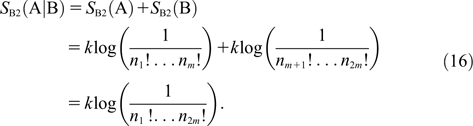
Now suppose we remove the barrier and allow the gases to mix. Following the reasoning given before, we can see that the occupancy numbers of cells for the mixed system AB will be essentially . So:

As , . So the entropy of mixing (i.e., ) is positive when we mix two samples of distinct gases.

6. Problems for the Usual Resolution of the Paradox

It is sometimes objected that while the division of W(D) by in the definition of S _B2 solves the problem, the physical justification behind this move is not obvious. The canonical response to this objection is that the division by arises because the permutation of two particles of the same type is not a real event, and it is thus a harbinger of quantum statistics (see, e.g., Schrödinger Reference Swendsen1946, 61). However, when W is defined as above, so that W(D) is the number of arrangements compatible with the distribution D, the claim that the division of W(D) by N! reflects that the fact that the permutation of two particles of the same type is not a real event makes no sense. Arrangements differ from one another only by a permutation of particles. So if we were to assume that a permutation of particles is not a real event, then we should in fact conclude that there is exactly one way to achieve every distribution, so we should in fact replace W(D) not by W(D)/N! but by a function that takes the value 1 for every possible D. And this would make the foregoing approach to defining entropy useless, since on this account, entropy would be 0 for every possible D.Footnote ¹⁰

But worrying about the physical justification of the division of S _B1 by is something of a red herring. If S _B2 was generally extensive, then the division of S _B1 by could perhaps be adequately justified on pragmatic grounds (e.g., Versteegh and Dieks Reference Versteegh and Dieks2011, 744). The real problem is that the division of S _B1 by does not fully solve the paradox, because S _B2, as it has been defined above, is itself not, in general, extensive.Footnote ¹¹ Consider a system (AB) consisting of a homogenous mix of two types of particles. Suppose we have 2N particles in total, N particles of type A, and N particles of type B. Then, the S _B2 of the system is:

So:

Now consider a similar system (2AB) of twice the size (i.e., occupying twice the volume and consisting of twice as many particles). The entropy of this system will be:

Assume that both systems are at equilibrium, so that both have a uniform distribution of particles over coordinate space and a Maxwell-Boltzmann distribution of particles over momentum space. So . So, since, :

So S _B2 is not, in general, extensive. This leads to a kind of “second-order” Gibbs paradox: suppose we have two samples of gas, A and B, each of which consists of 2N particles (N particles of type 1 and N particles of type 2). Prior to mixing S _B2 for the joint system will be:

whereas after mixing, S _B2 will be:

So (from the above considerations), . That is, there is a positive entropy of mixing when we mix two similar samples of gas, when each is composed of two types of particles.

However, it should be noted that although S _B2 is not, in general, extensive, it is approximately extensive when we are dealing with systems consisting of large numbers of particles (where we can use the Stirling approximation: ). And one might argue that this is all that is required: the requirement of extensivity is implied by the requirements of faithfulness, additivity, and indifference. But we only require statistical mechanical entropy to be faithful to thermodynamic entropy when we are dealing with systems consisting of large numbers of particles (since thermodynamics is only concerned with such systems). So, perhaps we should only require statistical mechanical entropy to be (approximately) extensive when we are dealing with such systems.Footnote ¹²

However, even if we accept that S _B2 need not be, in general, extensive, Swendsen (Reference Swendsen2006, Reference Van Kampen and Parry2008) has drawn attention to another version of the Gibbs paradox that arises when we consider the S _B2 of colloids. A colloid consists of a collection of microscopic particles of one substance homogeneously dispersed in another. Milk is a colloid: it consists of a collection of microscopic fat particles homogeneously dispersed in water. The particles in a colloid are distinguishable, since they contain “different numbers of atoms in different arrangements with different impurities” (Swendsen Reference Swendsen2006, 187). Using S _B2 as the definition of entropy, we find that there is a nonzero entropy of mixing when we mix two samples of the same colloid. Assume that we have two samples of a colloid, each consisting of N particles, and that every particle is distinct from every other (in the relevant sense: they are not macroscopically distinguishable, but they have different intrinsic properties). There are thus 2N different types of particles in total. In that case, , so dividing W(D) by will leave W(D) unaltered. So initially the entropy of the system is given by:

Now suppose we remove the barrier and allow the colloids to mix. Following the reasoning given before, we can see that the occupancy numbers of cells for the mixed system AB will be essentially . So:

As , . So the entropy of mixing (i.e., ) is positive when we mix two samples of the same colloid. As with the original paradox, this implies that there must be a decrease of statistical mechanical entropy when we insert a barrier to split a single volume of a colloid into two, and this would make violating the statistical mechanical analogue of the second law of thermodynamics trivial.

7. Generalized Boltzmann Entropy

One possible response to the second-order Gibbs paradoxes and to Swendsen's version of the paradox is to argue that they rest on a misapplication of S _B2. Recall that S _B2 was defined as:

where W is defined as:

and is the number of arrangements corresponding to the distribution D (given by the m-tuple ). This notion was defined with systems consisting of only a single type of particle in mind. If we are to consider systems consisting of k different types of particles, then a natural way to generalize W is as follows:

where N _i is the total number of particles of the ith type in the system, and n _i,j is the number of particles of the ith type in the jth coarse-grained cell. This gives the number of arrangements corresponding to the generalized distribution D _G. This is given by the km-tuple , which tells us, for each of the k types of particles, the number in each of the m coarse-grained cells. The generalized distribution (D _G) thus gives us more information than the distribution (D) (except when we have only a single type of particle, when they are the same): whereas D is insensitive to any permutations between particles (it tells us nothing about whether particle 1 is in cell 1 and particle 2 is in cell 2 or vice versa), D _G is only insensitive to permutations between particles of the same type.

This suggests that, if we are to use the Boltzmann entropy for systems consisting of more than one type of particle, we need to use the following “generalized” version of S _B2:

How does S _B2G fair with respect to the Gibbs paradox? Note that S _B2G = S _B2 in the case that we have only one type of particle (i.e., in the case in which S _B2 is extensive). So when we mix two samples of the same gas, S _B2G behaves in the same way as S _B2. So there is no increase in the value of S _B2G when we mix two samples of the same gas, as required.

Also, when we mix two samples (A and B) of distinct gases, there is an increase of S _B2G. Suppose, for concreteness, that A and B are samples of hydrogen and oxygen (respectively). We will again assume that the two samples have the same temperature, pressure, and volume and contain the same number (N) of particles. We will also assume that there are m accessible cells in each of the coarse-grained μ-spaces. The initial values of S _B2G are then as follows:

So the S _B2G of the joint system is:

After mixing the S_B2G of the system, AB is given by:

where n _H,1 is the number of hydrogen molecules in the first cell, and n _O,1 is the number of oxygen molecules in the first cell, and so on.

Ignoring the differences between the types of particles, the systems A and B are in equilibrium with each other before they are mixed (since they have the same volume, temperature, and pressure). So, if we ignore the differences between the types of particles, both the unmixed system A|B and the mixed system AB will have essentially the same (Maxwell-Boltzmann) distribution of particles over momentum space and also essentially the same (uniform) distribution of particles over coordinate space. So, n _H,1 + n _O,1 (for AB) will be approximately equal to n ₁ (for A|B), and so on. But for AB, both n _H,1 and n _O,1 will typically be greater than 0 and less than n ₁ (and similarly for n _H,2 and n _O,2, etc.; otherwise, the system would not have mixed). So S _B2G(AB) will be greater than S _B2G(A|B). (If a + b = c and a and b are both greater than 0, then c! > a!b!). Hence there is a positive entropy of mixing when we mix two samples of distinct gases, as required.

So S _B2G, like S _B2, solves the original version of the Gibbs paradox. But unlike S _B2, it also solves the second-order version of the paradox. Consider a system (AB) consisting of a homogenous mix of two types of particles. Suppose we have 2N particles in total, N particles of type A, and N particles of type B. Then, the S _B2G of the system is:

So:

Now consider a similar system (2AB) of twice the size (i.e., occupying twice the volume and consisting of twice as many particles). The entropy of this system will be:

Assume that both systems are at equilibrium, so that both have a uniform distribution of particles over coordinate space and a Maxwell-Boltzmann distribution of particles over momentum space. So . So:

So there is no second-order Gibbs paradox if we adopt S _B2G as the definition of entropy in statistical mechanics.

Finally, let's consider Swendsen's version of the Gibbs paradox. He noted that S _B2 (like S _B1) implies that there is a positive entropy of mixing when we mix two samples of a colloid: S _B2G evades this objection. We will assume (like Swendsen) that, in a colloid, every particle is distinct from every other particle. Suppose that initially sample A consists of k particles of type 1 through to k, and sample B consists of k particles of types through to 2k. We will also assume that there are m accessible cells in each of the coarse-grained μ-spaces. Then the values of S _B2G will initially be as follows:

So the S _B2G of the joint system is:

After mixing, the S _B2G of the system AB is given by:

Because there is only one of each type of particle, each n _i,j will be either 0 or 1 for both AB and A|B. So each n _i,j! will be 1 for both AB and A|B. So S _B2G(AB) will be equal to S _B2G(A|B). Hence there is no entropy of mixing when we mix two samples of colloid, as required.

However, this solution to Swendsen's version of the Gibbs paradox reveals that S _B2G is also not a satisfactory definition of entropy. For a system in which every particle is of a different type from every other (e.g., a colloid), each n _i,j in the definition of S _B2G will be either 0 or 1, as noted. This means that S _B2G will always be 0 for such a system, no matter what state the system is in. The analogous claim is of course far from true of thermodynamic entropy, so S _B2G is not a suitable counterpart to thermodynamic entropy. For example, consider a sample of gas in which every particle is of a different type from every other. Now consider two possible states of the gas: one in which it occupies a volume V (at temperature T and pressure P) and another in which it occupies volume 2V (at temperature T and pressure P). The thermodynamic entropy of the gas is of course higher in the second state. But S _B2G is 0 in both cases, since the number of particles of any given type that occupy the coarse-grained cells is 1 or 0 in both cases.

8. Summary

The usual resolution of the Gibbs paradox is to propose a new definition of statistical mechanical entropy (S _B2). However, it has been shown that if one does not generalize S _B2, then one can still generate “second-order” Gibbs paradoxes using this definition of entropy and that a Gibbs-style paradox arises in connection with the mixing of colloids. However, if one does generalize S _B2 in a natural way (to obtain S _B2G), then it implies that the entropy of a system of particles in which all the particles are distinct from one another (e.g., a colloid) is always zero. The usual resolution of the paradox is thus not satisfactory.