1. Introduction
Particle segregation impacts granular flows both in industry and in nature. For example, in the pharmaceutical industry, flow segregation of particles of different types is often undesirable, and homogeneous mixing is encouraged (Muzzio, Shinbrot & Glasser Reference Muzzio, Shinbrot and Glasser2002). In natural phenomena, such as debris flows, reverse grading takes place, in which higher concentrations of larger particles of the same material develop on top and in front of the flow (Armanini, Fraccarollo & Larcher Reference Armanini, Fraccarollo, Larcher and Anderson2005). This has important effects on the rheology of the mixture, altering parameters such as the depth and the velocity of the flow, on the characteristics and consequences of the impact of the flow on structures meant to confine it, and on the nature of the flow deposit when the flow comes to rest (Jakob & Hungr Reference Jakob and Hungr2005; Takahashi Reference Takahashi2014).
Many authors have observed that in inclined flows of binary mixtures of spheres that differ in both size and mass, two mechanisms appear to influence segregation: heavier particles tend to sink in a medium of lower average density, due to gravitational effects, while smaller particles tend to percolate downwards through interstices, due to geometrical effects, inducing larger particles to ride above them. Such observations are common to free-surface flows (e.g. Drahun & Bridgwater Reference Drahun and Bridgwater1983), rotating tumblers (e.g. Alonso, Satoh & Miyanami Reference Alonso, Satoh and Miyanami1991; Felix & Thomas Reference Felix and Thomas2004; Jain, Ottino & Lueptow Reference Jain, Ottino and Lueptow2005a ,Reference Jain, Ottino and Lueptow b ; Hill et al. Reference Hill, Fan, Zhang, Niekerk, Zastrow, Hagness and Bernhard2010) and rotating tubes (e.g. Metcalfe & Shattuck Reference Metcalfe and Shattuck1996). In our view, all of these experimental observations can be explained using modifications of the kinetic theory that we employ here.
Despite the importance of particle segregation in dense collisional particle flows, the theoretical framework for its description is still incomplete. Simple theories exist, based on continuum mixture theory (Atkin Reference Atkin1976), such as those described by Fan & Hill (Reference Fan and Hill2011), Gray & Ancey (Reference Gray and Ancey2011), Marks, Rognon & Einav (Reference Marks, Rognon and Einav2012) and Fan et al. (Reference Fan, Schlick, Umbanhowar, Ottino and Lueptow2014); these produce plausible predictions of species’ concentrations and mixture velocity, for appropriate choices of parameters. Our goal here is to make such predictions in the context of a theory that is based on measured particle properties, with coefficients that are given functions of the mixture volume fraction, and which incorporates a measure of the energy of the particle velocity fluctuations. The governing equations are based on the balances of mass, momentum and energy for the two species and the mixture. With respect to the predictions being sensitive to the properties of the particles and the governing equations being based on fundamental physical principals, our formulation differs from and, in our view, improves upon existing theories.
Larcher & Jenkins (Reference Larcher and Jenkins2013) formulated an approximate theory for steady fully developed flows of a binary mixture of inelastic spheres in the dense limit based on earlier work by Arnarson & Jenkins (Reference Arnarson and Jenkins2004). The segregation theory is appropriate for particles with relatively small differences in size and mass. They employed the extension of the kinetic theory of Garzo & Dufty (Reference Garzo and Dufty1999) for identical inelastic spheres by Jenkins (Reference Jenkins2007), who introduced an additional length scale into the expression for the rate of collisional energy dissipation to take into account correlated collisions and the formation of particle clusters (Jenkins & Berzi Reference Jenkins and Berzi2010). Larcher & Jenkins (Reference Larcher and Jenkins2013) predicted the species concentration, mixture concentration and mixture velocity, and compared the results with those obtained by Tripathi & Khakhar (Reference Tripathi and Khakhar2011) in numerical simulations.
Here, we extend the theory of Larcher & Jenkins (Reference Larcher and Jenkins2013) beyond the steady uniform state to include the description of time- or space-dependent segregation and predict the evolution in time or space of the relative concentrations of the two species. In doing this, we assume that the flow of the mixture reaches a fully developed state much more rapidly than do the concentrations of the two species. In dense flows, the rate at which segregation takes place is much slower than the rate at which momentum is transferred in the mixture. The former is proportional to the average distance between the edges of the spheres, the latter is inversely proportional to this distance. The model for the mixture is obtained from the balance of mixture mass, momentum and energy for a dense inclined flow. In such dense dissipative inclined flows, the concentration of the mixture is constant through most of the flow depth. The segregation is described using a kinetic theory developed for less dense flows of nearly elastic spheres.
We consider a mixture of spherical particles with two different radii,
 $r_{A}$
and
 $r_{B}$
, masses,
 $m_{A}$
and
 $m_{B}$
, number densities,
 $n_{A}$
and
 $n_{B}$
, and mass densities,
 ${\it\rho}_{A}=m_{A}n_{A}$
and
 ${\it\rho}_{B}=m_{B}n_{B}$
. We predict the profiles of mixture volume fraction,
 $c$
, mixture velocity,
 $u$
, and the evolution in time or space of the species concentration fractions,
 $c_{A}/c$
and
 $c_{B}/c$
, where
 $c_{A}=4{\rm\pi}n_{A}r_{A}^{3}/3$
,
 $c_{B}=4{\rm\pi}n_{B}r_{B}^{3}/3$
and
 $c=c_{A}+c_{B}$
, for various combinations of particle radii and particle masses. We compare their evolution in time with the results of discrete-element numerical simulations by Thornton et al. (Reference Thornton, Weinhart, Luding and Bokhove2012) and Weinhart, Luding & Thornton (Reference Weinhart, Luding, Thornton, Yu, Dong, Yang and Luding2013), and their evolution in space with the physical experiments of Savage & Lun (Reference Savage and Lun1988) and Wiederseiner et al. (Reference Wiederseiner, Andreini, Épely-Chauvin, Moser, Monnereau, Gray and Ancey2011). Finally, we show the evolution of segregation for spheres of the same size, but different masses, and indicate how particular combinations of radius and mass ratios result in an evolution towards a perfectly mixed state, whatever the initial condition of the mixture.
2. Balance equations
2.1. Segregation
The difference of mass balances of the two particle species
 $A$
and
 $B$
can be expressed as
 $$\begin{eqnarray}\frac{\partial }{\partial t}\left({\it\rho}_{A}-{\it\rho}_{B}\right)+\frac{\partial }{\partial x}\left({\it\rho}_{A}u_{A}-{\it\rho}_{B}u_{B}\right)+\frac{\partial }{\partial y}\left({\it\rho}_{A}v_{A}-{\it\rho}_{B}v_{B}\right)=0,\end{eqnarray}$$
where
 $u_{A}$
,
 $u_{B}$
,
 $v_{A}$
and
 $v_{B}$
are the velocity components along the flow, the direction of increasing
 $x$
, and across the flow, the direction of increasing
 $y$
, of particles of species
 $A$
and
 $B$
respectively. The mass-averaged components,
 $u$
and
 $v$
, of the velocity are given by
 $$\begin{eqnarray}{\it\rho}u={\it\rho}_{A}u_{A}+{\it\rho}_{B}u_{B}\quad \text{and}\quad {\it\rho}v={\it\rho}_{A}v_{A}+{\it\rho}_{B}v_{B},\end{eqnarray}$$
where the total density,
 ${\it\rho}$
, is the sum of the densities of the two species,
 ${\it\rho}={\it\rho}_{A}+{\it\rho}_{B}$
.
The components
 $\tilde{u} _{A}=u_{A}-u$
and
 $\tilde{v}_{A}=v_{A}-v$
of the diffusion velocities provide a measure of the velocity of segregation. Upon employing them in (2.1), we obtain
 $$\begin{eqnarray}\displaystyle & & \displaystyle \frac{\partial }{\partial t}\left({\it\rho}_{A}-{\it\rho}_{B}\right)+\frac{\partial }{\partial x}\left({\it\rho}_{A}-{\it\rho}_{B}\right)u+\frac{\partial }{\partial y}\left({\it\rho}_{A}-{\it\rho}_{B}\right)v\nonumber\\ \displaystyle & & \displaystyle \quad +\,\frac{\partial }{\partial x}\left({\it\rho}_{A}\tilde{u} _{A}-{\it\rho}_{B}\tilde{u} _{B}\right)+\frac{\partial }{\partial y}\left({\it\rho}_{A}\tilde{v}_{A}-{\it\rho}_{B}\tilde{v}_{B}\right)=0.\end{eqnarray}$$
Using
 ${\it\rho}_{A}\tilde{u} _{A}+{\it\rho}_{B}\tilde{u} _{B}=0$
and
 ${\it\rho}_{A}\tilde{v}_{A}+{\it\rho}_{B}\tilde{v}_{B}=0$
, (2.3) becomes
 $$\begin{eqnarray}\displaystyle & & \displaystyle \frac{\partial }{\partial t}\left({\it\rho}_{A}-{\it\rho}_{B}\right)+u\frac{\partial }{\partial x}\left({\it\rho}_{A}-{\it\rho}_{B}\right)+v\frac{\partial }{\partial y}\left({\it\rho}_{A}-{\it\rho}_{B}\right)\nonumber\\ \displaystyle & & \displaystyle \quad +\,\left({\it\rho}_{A}-{\it\rho}_{B}\right)\left(\frac{\partial u}{\partial x}+\frac{\partial v}{\partial y}\right)+2\frac{\partial }{\partial x}{\it\rho}_{A}\tilde{u} _{A}+2\frac{\partial }{\partial y}{\it\rho}_{A}\tilde{v}_{A}=0.\end{eqnarray}$$
In (2.4), the divergence of
 $(u,v)$
can be obtained from the mass balance for the mixture,
 $$\begin{eqnarray}\frac{\partial u}{\partial x}+\frac{\partial v}{\partial y}=-\frac{1}{{\it\rho}}\left(\frac{\partial {\it\rho}}{\partial t}+u\frac{\partial {\it\rho}}{\partial x}+v\frac{\partial {\it\rho}}{\partial y}\right),\end{eqnarray}$$
while
 $$\begin{eqnarray}{\it\rho}_{A}\tilde{u} _{A}=\frac{{\it\rho}_{A}{\it\rho}_{B}}{{\it\rho}}\left(\tilde{u} _{A}-\tilde{u} _{B}\right)\quad \text{and}\quad {\it\rho}_{A}\tilde{v}_{A}=\frac{{\it\rho}_{A}{\it\rho}_{B}}{{\it\rho}}\left(\tilde{v}_{A}-\tilde{v}_{B}\right).\end{eqnarray}$$
Then,
 $$\begin{eqnarray}\displaystyle & & \displaystyle {\it\rho}\frac{\partial }{\partial t}\left(\frac{{\it\rho}_{A}-{\it\rho}_{B}}{{\it\rho}}\right)+{\it\rho}u\frac{\partial }{\partial x}\left(\frac{{\it\rho}_{A}-{\it\rho}_{B}}{{\it\rho}}\right)+{\it\rho}v\frac{\partial }{\partial y}\left(\frac{{\it\rho}_{A}-{\it\rho}_{B}}{{\it\rho}}\right)\nonumber\\ \displaystyle & & \displaystyle \quad +\,2\frac{\partial }{\partial x}\left[\frac{{\it\rho}_{A}{\it\rho}_{B}}{{\it\rho}}\left(\tilde{u} _{A}-\tilde{u} _{B}\right)\right]+2\frac{\partial }{\partial y}\left[\frac{{\it\rho}_{A}{\it\rho}_{B}}{{\it\rho}}\left(\tilde{v}_{A}-\tilde{v}_{B}\right)\right]=0.\end{eqnarray}$$
The difference in the vector diffusion velocities is driven by gradients in the mixture pressure,
 $P$
, the kinetic energy of the velocity fluctuations, or mixture granular temperature,
 $T$
, and the number densities of the two species (Arnarson & Jenkins Reference Arnarson and Jenkins2004):
 $$\begin{eqnarray}\displaystyle \tilde{\boldsymbol{v}}_{A}-\tilde{\boldsymbol{v}}_{B} & = & \displaystyle -\frac{n^{2}}{n_{A}n_{B}}D_{AB}\left\{-\frac{{\it\rho}_{A}}{n{\it\rho}T}\boldsymbol{{\rm\nabla}}P+\frac{1}{nT}\left(n_{A}+2\frac{m_{A}}{m_{AB}}K_{AB}+K_{AA}\right)\boldsymbol{{\rm\nabla}}T\right.\nonumber\\ \displaystyle & & \displaystyle \left.+\,\frac{n_{A}}{nT}\left(\frac{\partial {\it\mu}_{A}}{\partial n_{A}}\boldsymbol{{\rm\nabla}}n_{A}+\frac{\partial {\it\mu}_{A}}{\partial n_{B}}\boldsymbol{{\rm\nabla}}n_{B}\right)+\frac{1}{T}K_{T}^{(A)}\boldsymbol{{\rm\nabla}}T\right\}.\end{eqnarray}$$
In this equation, the diffusion coefficient,
 $D_{AB}$
, is given by (Arnarson & Jenkins Reference Arnarson and Jenkins2004)
 $$\begin{eqnarray}D_{AB}\equiv \frac{3}{2ng_{AB}}\left(\frac{2Tm_{AB}}{{\rm\pi}m_{A}m_{B}}\right)^{1/2}\frac{1}{8r_{AB}^{2}},\end{eqnarray}$$
in which
 $m_{ij}=m_{i}+m_{j}$
and
 $r_{ij}=r_{i}+r_{j}$
, with
 $i,j=A$
or
 $B$
, are respectively the sums of the masses and radii and
 $g_{ij}$
are the radial distribution functions at collision for the components of the mixture:
 $$\begin{eqnarray}g_{ij}=\frac{1}{1-c}+\frac{3r_{i}r_{j}}{r_{ij}}\frac{{\it\xi}_{2}}{(1-c)^{2}}+2\left(\frac{r_{i}r_{j}}{r_{ij}}\right)^{2}\frac{{\it\xi}_{2}^{2}}{(1-c)^{3}},\end{eqnarray}$$
with
 ${\it\xi}_{2}\equiv 4{\rm\pi}(n_{A}r_{A}^{2}+n_{B}r_{B}^{2})/3$
and
 $K_{ij}=2{\rm\pi}r_{ij}^{3}n_{i}n_{j}g_{ij}/3$
. The mixture pressure is the sum of the partial pressures of the two particle species,
 $p_{A}$
and
 $p_{B}$
, given by (Arnarson & Jenkins Reference Arnarson and Jenkins2004)
 $$\begin{eqnarray}p_{A}=\left(n_{A}+K_{AA}+K_{AB}\right)T\quad \text{and}\quad p_{B}=\left(n_{B}+K_{BB}+K_{AB}\right)T.\end{eqnarray}$$
These can be used to evaluate the first prefactor of the gradient of the granular temperature in (2.8),
 $$\begin{eqnarray}\left(n_{A}+2\frac{m_{A}}{m_{AB}}K_{AB}+K_{AA}\right)\boldsymbol{{\rm\nabla}}T=\frac{p_{A}}{T}\boldsymbol{{\rm\nabla}}T-\frac{m_{B}-m_{A}}{m_{AB}}K_{AB}\boldsymbol{{\rm\nabla}}T.\end{eqnarray}$$
Approximate expressions for the mass densities, the gradient of the chemical potential,
 ${\it\mu}_{A}$
, and the coefficient of thermal diffusion,
 $K_{T}^{(A)}$
, are given in appendix A, in the context of a theory for mixtures in which it is assumed that the radii and the masses of the two types of spheres do not differ by much. Arnarson & Jenkins (Reference Arnarson and Jenkins2004) and Larcher & Jenkins (Reference Larcher and Jenkins2013) provide complete expressions for the chemical potential and the coefficient of thermal diffusion and derive the approximations. In the approximate theory,
 ${\it\delta}r\equiv (r_{A}/r_{B})-1$
and
 ${\it\delta}m\equiv (m_{A}-m_{B})/m_{AB}$
measure the differences in size and mass, and the quantity
 $X\equiv (n_{A}-n_{B})/(2n)$
measures the segregation.
As indicated in appendix A, the approximate form of the mass balance, (2.7), phrased in terms of these variables is
 $$\begin{eqnarray}\displaystyle & & \displaystyle {\it\rho}\frac{\partial X}{\partial t}+{\it\rho}u\frac{\partial X}{\partial x}+{\it\rho}v\frac{\partial X}{\partial y}+\frac{\partial }{\partial x}\left[\frac{m_{A}n}{4}\left(1-4X^{2}\right)\left(\tilde{u} _{A}-\tilde{u} _{B}\right)\right]\nonumber\\ \displaystyle & & \displaystyle \quad +\,\frac{\partial }{\partial y}\left[\frac{m_{A}n}{4}\left(1-4X^{2}\right)\left(\tilde{v}_{A}-\tilde{v}_{B}\right)\right]=0,\quad\end{eqnarray}$$
where
 $$\begin{eqnarray}\displaystyle \tilde{\boldsymbol{v}}_{A}-\tilde{\boldsymbol{v}}_{B}=-D_{AB}\hspace{-2.0pt}\left[({\it\Gamma}_{1}{\it\delta}m+R_{1}{\it\delta}r)\frac{\boldsymbol{{\rm\nabla}}T}{T}-({\it\Gamma}_{2}{\it\delta}m+R_{2}{\it\delta}r)\frac{m_{AB}\boldsymbol{g}\cos {\it\phi}}{2T}+\frac{\boldsymbol{{\rm\nabla}}X}{0.25-X^{2}}\right]\!,\qquad & & \displaystyle\end{eqnarray}$$
in which
 $$\begin{eqnarray}\displaystyle & \displaystyle D_{AB}=\frac{{\rm\pi}^{1/2}}{16}\frac{r_{AB}}{G}\left(\frac{2T}{m_{AB}}\right)^{1/2}, & \displaystyle\end{eqnarray}$$
 $$\begin{eqnarray}\displaystyle & \displaystyle {\it\Gamma}_{1}=\frac{179}{29}G+\frac{105}{116}\doteq 6.17G, & \displaystyle\end{eqnarray}$$
 $$\begin{eqnarray}\displaystyle & \displaystyle {\it\Gamma}_{2}=2,\quad R_{2}=-\frac{12cH}{1+4G+4cH}\doteq -3 & \displaystyle\end{eqnarray}$$
and
 $$\begin{eqnarray}\displaystyle R_{1}=\frac{5}{58}\left[2+\frac{c(3-c)}{2-c}-\frac{12}{5}G\right]+2G\left[3+\frac{c(3-c)}{2-c}\right]-\frac{12cH(1+4G)}{1+4G+4cH}\doteq -4.35G. & & \displaystyle \nonumber\\ \displaystyle & & \displaystyle\end{eqnarray}$$
Here, the functions
 $G$
and
 $H$
are related to the radial distribution function of the mixture, regarded as a single species with mass
 $m_{AB}/2$
and
 $r_{AB}/2$
(Torquato Reference Torquato1995):
 $$\begin{eqnarray}G=5.69c\frac{c_{M}-0.49}{c_{M}-c}\end{eqnarray}$$
and
 $$\begin{eqnarray}H\equiv \frac{\text{d}G}{\text{d}c}=G\frac{c_{M}}{c(c_{M}-c)},\end{eqnarray}$$
in which
 $c_{M}$
is the value of the mixture concentration at which these functions become singular (Mitarai & Nakanishi Reference Mitarai and Nakanishi2007). The separation between the edges of the fictive spheres of the mixture is inversely proportional to
 $G$
. The approximations in (2.16)–(2.18) apply at a value of 0.55 of the mixture volume fraction. Here, we take the value of the singularity,
 $c_{M}$
, to be 0.58. This provides the best fit to the simulations of Tripathi & Khakhar (Reference Tripathi and Khakhar2011), which were carried out with particles that had the same inertial and contact properties as those employed by Silbert et al. (Reference Silbert, Ertas, Grest, Halsey, Levine and Plimpton2001), and which are often adopted by others. Results of the fit are shown in figure 2 of Larcher & Jenkins (Reference Larcher and Jenkins2013).
Equation (2.14) indicates that inhomogeneity in the species’ concentrations results from an imbalance between the gradient of the difference in the species’ number fractions and a segregation flux that contains contributions from both the gradient of the mixture temperature and gravity. Each contribution to the segregation flux is linear in the differences in the size and mass of the two species, with coefficients that are functions of the mixture concentration.
2.2. Dense flows of the mixture
For the flow of the dense mixture, we employ an extension of the kinetic theory that incorporates an additional length scale in the rate of collisional dissipation that is associated with chains or clusters of a characteristic size in the flow. This length scale is determined in a phenomenological balance between the orienting influence of the mean shear rate and the randomizing influence of the collisions. The balance of fluctuation energy, used with the determination of the length scale, provides relations that are, in the collisional regime, the equivalents of purely phenomenological relations that have recently been employed for dense flows (GDR MiDi 2004; Jop, Forterre & Pouliquen Reference Jop, Forterre and Pouliquen2005). Here, we show the expressions for the mixture quantities needed to predict the segregation, and the briefest sketch of their derivation. Larcher & Jenkins (Reference Larcher and Jenkins2013) provide the details.
The transport coefficients of the mixture are given by the theory of Garzo & Dufty (Reference Garzo and Dufty1999) for identical very dissipative spheres, modified in the way introduced by Arnarson & Jenkins (Reference Arnarson and Jenkins2004) for binary mixtures of nearly elastic spheres that do not differ much in size and mass. From this point on, we consider the mixture to have achieved a steady uniform state that varies only with the coordinate
 $y$
across the flow, with its upper surface at
 $y=h$
.
The profile for the granular temperature
 $T$
results from the component of the mixture momentum balance across the flow and the fact that in such dense flows, the mixture concentration is uniform across the flow (Silbert et al.
Reference Silbert, Ertas, Grest, Halsey, Levine and Plimpton2001):
 $$\begin{eqnarray}T=\frac{m_{AB}(h-y)}{4(1+e)G}g\cos {\it\phi}\left(1+2X{\it\delta}m\right)\!.\end{eqnarray}$$
The uniform mixture concentration is related to the angle of inclination of the flow and the particle parameters. This relationship is derived from the energy balance for the mixture, in which the rate of work of the mixture shear stress through the gradients of the mixture velocity is balanced by the rate of collisional dissipation. In this balance, the determination of the additional length is used in the rate of collisional dissipation. One result is an expression for
 $G$
in terms of the angle of inclination, properties of the mixture and a coefficient of restitution
 $e$
:
 $$\begin{eqnarray}G=\left\{\frac{4J}{5{\rm\pi}^{1/2}}\frac{1}{1+e}\left[\frac{15}{J}\frac{(1-e^{2})}{{\it\alpha}}\right]^{1/3}\frac{1}{\tan {\it\phi}}\right\}^{9}\left[1+3X\left({\it\delta}r+{\it\delta}m\right)\right],\end{eqnarray}$$
where
 ${\it\alpha}$
, a coefficient of order one in the relation that determines the additional length scale, is taken here to be 0.5, and
 $J$
is a coefficient in the mixture shear stress,
 $$\begin{eqnarray}J=\frac{(1+e)}{2}+\frac{{\rm\pi}}{4}\frac{(3e-1)(1+e)^{2}}{\left[24-(1-e)(11-e)\right]}.\end{eqnarray}$$
This form of
 $J$
is appropriate for dense flows of a single species of very dissipative spheres and incorporates the dependence on the coefficient of restitution determined by Garzo & Dufty (Reference Garzo and Dufty1999). We incorporate friction in the particle interactions through the introduction of an effective coefficient of restitution in the translational energy equation (Jenkins & Zhang Reference Jenkins and Zhang2010) and avoid the necessity of introducing an additional balance equation for the energy of the rotational velocity fluctuations. This effective coefficient accounts for energy lost to the fluctuations in translation velocity due to both their conversion to rotational velocity fluctuations and their dissipation due to sliding friction or tangential restitution. Larcher & Jenkins (Reference Larcher and Jenkins2013) outline its derivation in an appendix. With (2.22), (2.19) may be inverted to give the desired relation
 $$\begin{eqnarray}c=\frac{c_{M}G}{G+5.69\left(c_{M}-0.49\right)}.\end{eqnarray}$$
The velocity of the mixture,
 $u$
, follows from the balance of mixture momentum along the flow and the relationship between the mixture shear stress and the mixture velocity gradient. When the latter is integrated, it provides
 $$\begin{eqnarray}u=u_{0}+\frac{5{\rm\pi}^{1/2}}{6J}\frac{1}{r_{AB}}\left(\frac{1+e}{2G}g\cos {\it\phi}\right)^{1/2}\left[h^{3/2}-(h-y)^{3/2}\right]\tan {\it\phi}(1-X{\it\delta}r),\end{eqnarray}$$
where the subscript
 $0$
indicates a quantity evaluated at the base and
 $u_{0}$
is the slip velocity. In what follows, we adopt the approximation,
 $u_{0}=0$
, since it does not affect significantly the prediction of granular segregation. Larcher & Jenkins (Reference Larcher and Jenkins2013) provide the details of the determination of the slip velocity as a function of the bumpiness, the granular temperature, the angle of inclination and the effective coefficient of restitution.
Finally, because by (2.13) and (2.14) derivatives of
 $X$
with respect to
 $y$
are proportional to small quantities,
 $X$
may be replaced by its depth average,
 $\bar{X}$
, whenever it multiplies
 ${\it\delta}r$
or
 ${\it\delta}m$
, as in (2.21), (2.22) and (2.25).
3. Evolution in time and space
3.1. Uniform time-dependent segregation
In the case of uniform time-dependent segregation, with the
 $y$
-axis normal to the flow and directed upward, (2.13) reduces to
 $$\begin{eqnarray}{\it\rho}\frac{\partial X}{\partial t}+\frac{\partial }{\partial y}\left[\frac{m_{A}n}{4}\left(1-4X^{2}\right)\left(\tilde{v}_{A}-\tilde{v}_{B}\right)\right]=0.\end{eqnarray}$$
Therefore,
 $$\begin{eqnarray}\displaystyle & & \displaystyle m_{AB}n\frac{\partial X}{\partial t}-\frac{\partial }{\partial y}\left\{\frac{m_{A}n}{2}\left(1-4X^{2}\right)D_{AB}\left[\left({\it\Gamma}_{1}{\it\delta}m+R_{1}{\it\delta}r\right)\frac{1}{T}\frac{\partial T}{\partial y}\right.\right.\nonumber\\ \displaystyle & & \displaystyle \quad \left.\left.+\,({\it\Gamma}_{2}{\it\delta}m+R_{2}{\it\delta}r)\frac{m_{AB}g\cos {\it\phi}}{2T}+\frac{4}{1-4X^{2}}\frac{\partial X}{\partial y}\right]\right\}=0,\qquad\end{eqnarray}$$
in which
 $D_{AB}$
is given by (2.15). When (2.21) for
 $T$
in the dense inclined flow is employed in this equation, it becomes
 $$\begin{eqnarray}\displaystyle \frac{\partial X}{\partial t} & = & \displaystyle \frac{r_{AB}\left({\rm\pi}g\cos {\it\phi}\right)^{1/2}}{128G^{3/2}}\left(\frac{2}{1+e}\right)^{1/2}\frac{\partial }{\partial y}\left[(h-y)^{1/2}\left\{\left[\left(2(1+e)G{\it\Gamma}_{2}-{\it\Gamma}_{1}\right){\it\delta}m\right.\right.\right.\nonumber\\ \displaystyle & & \displaystyle \left.\left.\left.+\,\left(2(1+e)GR_{2}-R_{1}\right){\it\delta}r\right]\frac{1-4X^{2}}{h-y}+4\frac{\partial X}{\partial y}\right\}\hspace{-1.5pt}\right]\!.\qquad\end{eqnarray}$$
We note that because of the dependence of the mixture temperature on
 $G$
and the approximations in (2.16) through (2.18), the terms in the segregation flux are all proportional to
 $G$
. If lengths are normalized by the height
 $h$
and time by
 $(r_{AB}/g)^{1/2}$
, then, with
 $z\equiv y/h$
and
 ${\it\tau}\equiv t/(r_{AB}/g)^{1/2}$
,
 $$\begin{eqnarray}\displaystyle \frac{\partial X}{\partial {\it\tau}} & = & \displaystyle \left(\frac{r_{AB}}{h}\right)^{3/2}\frac{\left({\rm\pi}\cos {\it\phi}\right)^{1/2}}{128G^{3/2}}\left(\frac{2}{1+e}\right)^{1/2}\frac{\partial }{\partial z}\left[(1-z)^{1/2}\left\{\left[\left(2(1+e)G{\it\Gamma}_{2}-{\it\Gamma}_{1}\right){\it\delta}m\right.\right.\right.\nonumber\\ \displaystyle & & \displaystyle \left.\left.\left.+\,\left(2(1+e)GR_{2}-R_{1}\right){\it\delta}r\right]\frac{1-4X^{2}}{1-z}+4\frac{\partial X}{\partial z}\right\}\hspace{-1.5pt}\right]\!.\qquad\end{eqnarray}$$
The form of (3.4) ensures that if the vertical flux vanishes at
 $z=0$
and
 $z=1$
, the integral of
 $X$
through the depth of the flow is constant in time. However, given the definition of
 $X$
in (A 5), this conservation is not compatible with the conservation of the total number of particles of the two species. This is because the depth average of a concentration fraction is not equal to the ratio of the depth averages of its numerator and denominator. A similar issue occurs in the context of the steady segregation problem (Xu, Louge & Reeves Reference Xu, Louge and Reeves2003; Larcher & Jenkins Reference Larcher and Jenkins2013). Therefore, in order to conserve the total number of particles, there and here, a new variable,
 ${\it\zeta}\equiv Xn/\bar{n}$
, is introduced, where the overbar indicates an average through the flow depth. Then,
 $$\begin{eqnarray}\bar{{\it\zeta}}\equiv \frac{1}{2}\left(\frac{\bar{n}_{A}}{\bar{n}}-\frac{\bar{n}_{B}}{\bar{n}}\right)=\frac{1}{2}\left(\frac{N_{A}}{N}-\frac{N_{B}}{N}\right),\end{eqnarray}$$
where
 $N_{A}$
and
 $N_{B}$
are the total numbers of particles of
 $A$
and
 $B$
respectively, and
 $N=N_{A}+N_{B}$
. The total number fraction
 $f_{A}=N_{A}/N$
or, equivalently, the total volume fraction
 $$\begin{eqnarray}\frac{V_{A}}{V}=\frac{\bar{c}_{A}}{\bar{c}}=\frac{f_{A}(r_{A}/r_{B})^{3}}{1-f_{A}+f_{A}(r_{A}/r_{B})^{3}}\end{eqnarray}$$
of type
 $A$
particles is known and conserved during the time evolution of the solution.
The variables
 ${\it\zeta}$
and
 $X$
can be related through known quantities by
 $$\begin{eqnarray}{\it\zeta}=\frac{2cX}{{\hat{c}}_{A}+{\hat{c}}_{B}+2\left({\hat{c}}_{A}-{\hat{c}}_{B}\right)X}\end{eqnarray}$$
or
 $$\begin{eqnarray}X=\frac{\left({\hat{c}}_{A}+{\hat{c}}_{B}\right){\it\zeta}}{2\left[c-\left({\hat{c}}_{A}-{\hat{c}}_{B}\right){\it\zeta}\right]}\,\doteq \,\frac{\left({\hat{c}}_{A}+{\hat{c}}_{B}\right)}{2c}{\it\zeta},\end{eqnarray}$$
where
 $$\begin{eqnarray}{\hat{c}}_{A}\equiv \frac{\bar{n}}{\bar{n}_{A}}\bar{c}_{A}\quad \text{and}\quad {\hat{c}}_{B}\equiv \frac{\bar{n}}{\bar{n}_{B}}\bar{c}_{B}.\end{eqnarray}$$
We employ the approximation in (3.8) to express (3.4) in terms of
 ${\it\zeta}$
:
 $$\begin{eqnarray}\displaystyle \text{}\frac{\partial {\it\zeta}}{\partial {\it\tau}} & = & \displaystyle \left(\frac{r_{AB}}{h}\right)^{3/2}\frac{\left({\rm\pi}\cos {\it\phi}\right)^{1/2}}{128G^{3/2}}\left(\frac{2}{1+e}\right)^{1/2}\frac{2c}{\left({\hat{c}}_{A}+{\hat{c}}_{B}\right)}\nonumber\\ \displaystyle & & \displaystyle \times \,\frac{\partial }{\partial z}\left\{\frac{\left[\left(2(1+e)G{\it\Gamma}_{2}-{\it\Gamma}_{1}\right){\it\delta}m+\left(2(1+e)GR_{2}-R_{1}\right){\it\delta}r\right]}{(1-z)^{1/2}}\right.\nonumber\\ \displaystyle & & \displaystyle \times \left.\left[1-\frac{\left({\hat{c}}_{A}+{\hat{c}}_{B}\right)^{2}}{c^{2}}{\it\zeta}^{2}\right]+2(1-z)^{1/2}\frac{\left({\hat{c}}_{A}+{\hat{c}}_{B}\right)}{c}\frac{\partial {\it\zeta}}{\partial z}\right\}.\end{eqnarray}$$
Then, the integral of
 ${\it\zeta}$
through the depth of the flow is approximately constant in time and initial conditions that involve the number fractions or volume fractions can be specified for it.
3.2. Steady longitudinal segregation
Lengths associated with the evolution of segregation are, typically, significantly larger than the flow depth, so we assume that streamwise derivatives in the difference of the diffusion velocities are negligible compared with cross-stream derivatives. Then, for steady longitudinal segregation,
 $X=X(y,x)$
, with the
 $x$
-axis along the flow and the
 $y$
-axis normal to the flow and directed upward, (2.13) assumes the form
 $$\begin{eqnarray}\displaystyle {\it\rho}u\frac{\partial }{\partial x}\left(\frac{{\it\rho}_{A}-{\it\rho}_{B}}{{\it\rho}}\right)+2\frac{\partial }{\partial y}\left[\frac{{\it\rho}_{A}{\it\rho}_{B}}{{\it\rho}}\left(\tilde{v}_{A}-\tilde{v}_{B}\right)\right]=0. & & \displaystyle\end{eqnarray}$$
At lowest order in
 ${\it\delta}r$
and
 ${\it\delta}m$
,
 $$\begin{eqnarray}\displaystyle & & \displaystyle \frac{m_{AB}}{2}\frac{6{\it\nu}}{{\rm\pi}r_{AB}^{3}}u\frac{\partial X}{\partial x}-\frac{\partial }{\partial y}\left\{\frac{m_{A}n}{4}\left(1-4X^{2}\right)\right.D_{AB}\left[\left({\it\Gamma}_{1}{\it\delta}m+R_{1}{\it\delta}r\right)\frac{1}{T}\frac{\partial T}{\partial y}\right.\nonumber\\ \displaystyle & & \displaystyle \quad \left.+\,({\it\Gamma}_{2}{\it\delta}m+R_{2}{\it\delta}r)\frac{m_{AB}g\cos {\it\phi}}{2T}\left.+\frac{4}{1-4X^{2}}\frac{\partial X}{\partial y}\right]\right\}=0.\end{eqnarray}$$
With (2.25),
 $$\begin{eqnarray}\displaystyle & & \displaystyle \left[h^{3/2}-(h-y)^{3/2}\right]\tan {\it\phi}\frac{\partial X}{\partial x}=\frac{3J}{160}\frac{1}{(1+e)}\frac{r_{AB}^{2}}{G}\frac{\partial }{\partial y}\left[\left(h-y\right)^{1/2}\right.\nonumber\\ \displaystyle & & \displaystyle \quad \times \,\left.\left\{\left[2(1+e)G(2{\it\delta}m+R_{2}{\it\delta}r)-\left({\it\Gamma}_{1}{\it\delta}m+R_{1}{\it\delta}r\right)\right]\frac{1-4X^{2}}{h-y}+4\frac{\partial X}{\partial y}\right\}\right].\end{eqnarray}$$
If lengths are normalized by the flow depth,
 $h$
, then, with
 $z\equiv y/h$
and
 $\ell \equiv x/h$
,
 $$\begin{eqnarray}\displaystyle & & \displaystyle \left[1-(1-z)^{3/2}\right]\tan {\it\phi}\frac{\partial X}{\partial \ell }=\frac{3J}{160(1+e)}\left(\frac{r_{AB}}{h}\right)^{2}\frac{1}{G}\frac{\partial }{\partial z}\left[\left(1-z\right)^{1/2}\right.\nonumber\\ \displaystyle & & \displaystyle \quad \times \,\left.\left\{\left[2(1+e)G(2{\it\delta}m+R_{2}{\it\delta}r)-\left({\it\Gamma}_{1}{\it\delta}m+R_{1}{\it\delta}r\right)\right]\frac{1-4X^{2}}{1-z}+4\frac{\partial X}{\partial z}\right\}\right].\end{eqnarray}$$
In analogy with the uniform time-dependent segregation problem described above, the approximation in (3.8) is employed to express (3.14) in terms of
 ${\it\zeta}$
:
 $$\begin{eqnarray}\displaystyle & & \displaystyle \left[1-(1-z)^{3/2}\right]\tan {\it\phi}\frac{\left({\hat{c}}_{A}+{\hat{c}}_{B}\right)}{2\bar{c}}\frac{\partial {\it\zeta}}{\partial \ell }=\frac{3J}{160(1+e)}\left(\frac{r_{AB}}{h}\right)^{2}\frac{1}{G}\nonumber\\ \displaystyle & & \displaystyle \quad \times \,\frac{\partial }{\partial z}\left\{\frac{\left[2(1+e)G(2{\it\delta}m+R_{2}{\it\delta}r)-\left({\it\Gamma}_{1}{\it\delta}m+R_{1}{\it\delta}r\right)\right]}{\left(1-z\right)^{1/2}}\right.\nonumber\\ \displaystyle & & \displaystyle \quad \times \left.\left[1-\frac{\left({\hat{c}}_{A}+{\hat{c}}_{B}\right)}{\bar{c}^{2}}^{2}{\it\zeta}^{2}\right]+2\left(1-z\right)^{1/2}\frac{\left({\hat{c}}_{A}+{\hat{c}}_{B}\right)}{\bar{c}}\frac{\partial {\it\zeta}}{\partial z}\right\}.\end{eqnarray}$$
However, the use of the approximation between
 $X$
and
 ${\it\zeta}$
of (3.8) in the correction for the differences in mass and radius in (2.22) is too crude for an accurate determination of the mixture volume fraction. Because Larcher & Jenkins (Reference Larcher and Jenkins2013) show that the use of the exact relation between
 $X$
in
 ${\it\zeta}$
in the correction results in little or no change from the single-species volume fraction, we use the uncorrected mixture volume fraction in what follows. Finally, we note that in steady longitudinal segregation, the quantities that are conserved are the fluxes of each species, i.e.
 $\int _{0}^{1}c_{A}u\,\text{d}z$
and
 $\int _{0}^{1}c_{B}u\,\text{d}z$
. As a consequence of the non-uniformity of the velocity across the flow, the depth-integrated concentration of each species may change with the longitudinal coordinate
 $\ell$
, up to the point at which segregation ceases (e.g. figure 5
b).
4. Comparison with experiments and simulations
4.1. Thornton et al. (Reference Thornton, Weinhart, Luding and Bokhove2012) simulations
Thornton et al. (Reference Thornton, Weinhart, Luding and Bokhove2012) performed chute-flow simulations over a rigid bumpy base using the discrete particle method for several bi-disperse systems with different size ratios. Their simulations take place in a periodic box inclined at an angle of
 $25^{\circ }$
to the horizontal. They use 5000 small particles and choose the number of the large ones in order that the total volumes of large and small spheres are equal. They show the time evolution of the vertical centres of mass (COMs) of the small and large particles as a function of the size ratio. Starting from a uniformly distributed mixture, the COM of the small particles decreases in time, while the COM of the large ones increases. The position of the COM has a steep rate of change at the beginning of the simulation and, later, tends to an asymptote. The larger the size ratio, the shorter the time needed by the COM to reach a constant value, i.e. for segregation to reach the steady state. The flow is rather dense, with a volume concentration of the mixture that is relatively constant and significatively above 0.5, with the exception of two thin layers at the bottom and at the top of the flow.
In applying kinetic theory, we assume a dense flow with a constant concentration, evaluated through (2.22) and (2.24), with
 ${\it\alpha}=0.5$
,
 $c_{M}=0.58$
,
 $e=0.65$
,
 $V_{A}/V=0.5$
, and
 $\bar{X}$
is related to
 $\bar{{\it\zeta}}$
through the approximate relation given by (3.8) or, equivalently, by
 $$\begin{eqnarray}\bar{X}\,\doteq \,0.5\left[V_{A}/V+\left(1-V_{A}/V\right)\left(r_{A}/r_{B}\right)^{3}\right]\left[1+(r_{B}/r_{A})^{3}\right]\bar{{\it\zeta}}.\end{eqnarray}$$
Because the integral of
 ${\it\zeta}$
through the flow depth is approximately constant in time and given (3.5), we have in (4.1)
 $$\begin{eqnarray}\bar{{\it\zeta}}=f_{A}-0.5=\frac{1}{2}\frac{V_{A}/V-\left(1-V_{A}/V\right)\left(r_{A}/r_{B}\right)^{3}}{V_{A}/V+\left(1-V_{A}/V\right)\left(r_{A}/r_{B}\right)^{3}}.\end{eqnarray}$$
The evolution of the segregation is then obtained by solving (3.10) with the Matlab embedded solver pdepe, suitable for initial boundary value problems for parabolic–elliptic partial differential equations in one space-like and one time-like variable. The initial condition is given by a uniformly mixed dispersion of spheres, with
 ${\it\zeta}=f_{A}-0.5$
throughout the flow depth, while the two boundary conditions require the total flux,
 $$\begin{eqnarray}\displaystyle & & \displaystyle \frac{\left[2(1+e)G{\it\Gamma}_{2}-{\it\Gamma}_{1}\right]{\it\delta}m+\left[2(1+e)GR_{2}-R_{1}\right]{\it\delta}r}{(1-z)^{1/2}}\nonumber\\ \displaystyle & & \displaystyle \quad \times \left[1-\frac{\left({\hat{c}}_{A}+{\hat{c}}_{B}\right)^{2}}{\bar{c}^{2}}{\it\zeta}^{2}\right]+2(1-z)^{1/2}\frac{\left({\hat{c}}_{A}+{\hat{c}}_{B}\right)}{\bar{c}}\frac{\partial {\it\zeta}}{\partial z},\end{eqnarray}$$
to vanish at the base,
 $z=0$
, and at the top,
 $z=1$
.
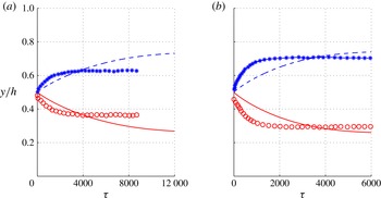
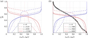
In figure 1, we show the time evolution of the positions of the COMs of the large and small spheres for two radius ratios and compare the results with the simulations of Thornton et al. (Reference Thornton, Weinhart, Luding and Bokhove2012). The agreement between the two approaches is relatively good. We predict a faster and sharper segregation when the radius ratio is larger; however, we reach the steady state in slightly longer time and predict a less diffuse segregation compared with the simulations (figure 2
b), similarly to what was obtained previously (Larcher & Jenkins Reference Larcher and Jenkins2013). We note that our asymptotic uniform state for
 $r_{A}/r_{B}=1.1$
differs from that of Thornton et al. (Reference Thornton, Weinhart, Luding and Bokhove2012), but agrees with the steady state obtained by Tripathi & Khakhar (Reference Tripathi and Khakhar2011).
Predicted COMs of large spheres (dashed blue) and small spheres (solid red) and those measured by Thornton et al. (Reference Thornton, Weinhart, Luding and Bokhove2012) (large spheres, blue stars; small spheres, red circles) for two radius ratios and the same material density: (a)
 $r_{A}/r_{B}=1.1$
,
 $m_{A}/m_{B}=(1.1)^{3}$
; (b)
 $r_{A}/r_{B}=1.3$
,
 $m_{A}/m_{B}=(1.3)^{3}$
. The other simulation parameters are
 ${\it\phi}=25^{\circ }$
,
 $e=0.65$
,
 $V_{A}/V=0.5$
and
 $h/r_{AB}=20$
. The vertical axes are the same in the two figures.

Predicted relative concentration profiles of large spheres (increasing functions, blue lines) and small spheres (decreasing functions, red lines) for two radius ratios at four equally spaced steps
 ${\rm\Delta}{\it\tau}$
of dimensionless time units, from the initial state to the steady state: (a)
 $r_{A}/r_{B}=1.1$
, (b)
 $r_{A}/r_{B}=1.3$
. The profile of steady relative concentration for the small spheres in the Thornton et al. (Reference Thornton, Weinhart, Luding and Bokhove2012) simulation is given in (b) for comparison (black circles). The simulation parameters are
 ${\it\phi}=25^{\circ }$
,
 $e=0.65$
,
 $m_{A}/m_{B}=(r_{A}/r_{B})^{3}$
,
 $V_{A}/V=0.5$
and
 $h/r_{AB}=20$
. The vertical axes are the same in the two figures.

In figure 2 we show, for the same radius ratios, the time evolution of the relative concentration profiles,
 $c_{A}/c$
and
 $c_{B}/c$
, from an initial state, in which the two species are perfectly mixed, to a steady state, with only large particles in the top layers and a clear dominance of small particles at the bottom, but some large particles, nonetheless, still present.
4.2. Wiederseiner et al. (Reference Wiederseiner, Andreini, Épely-Chauvin, Moser, Monnereau, Gray and Ancey2011) experiments
Wiederseiner et al. (Reference Wiederseiner, Andreini, Épely-Chauvin, Moser, Monnereau, Gray and Ancey2011) performed laboratory experiments on a chute with an inclination
 ${\it\phi}=29^{\circ }$
. They used a binary mixture of glass beads with a radius ratio of
 $r_{A}/r_{B}=2$
and showed how the relative concentration of the two species evolved from a position
 $x/L=0.01$
very close to the origin of the chute to the section at
 $x/L=1$
where the asymptotic solution was reached. They observed that the evolution of segregation was greatly influenced by the inflow rates.
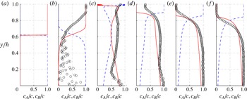
The results, presented in dimensionless form in figure 3, show good agreement, even if a slightly longer distance was needed in order to reach the steady state.
Predicted evolution with distance of the relative concentration profiles of large spheres (dashed blue lines) and small spheres (solid red lines) at six different locations between the origin and the section at which the asymptotic solution is established: (a)
 $x/L=0$
, (b)
 $x/L=0.01$
, (c)
 $x/L=0.25$
, (d)
 $x/L=0.5$
, (e)
 $x/L=0.75$
, (f)
 $x/L=1$
. The simulation parameters are
 ${\it\phi}=29^{\circ }$
,
 $e=0.65$
,
 $r_{A}/r_{B}=2$
,
 $m_{A}/m_{B}=(r_{A}/r_{B})^{3}$
,
 $V_{A}/V=0.62$
and
 $h/r_{AB}=16$
. The profile of the relative concentration of small spheres in the experiments of Wiederseiner et al. (Reference Wiederseiner, Andreini, Épely-Chauvin, Moser, Monnereau, Gray and Ancey2011) (black circles) is given for comparison. The vertical axes are the same in all of the figures.

4.3. Savage & Lun (Reference Savage and Lun1988) experiments
Savage & Lun (Reference Savage and Lun1988) performed experiments on size segregation in inclined chute flows almost three decades ago, but their findings are still among the most cited on granular segregation. Although they are known as the basis for the random fluctuating sieve model, they also provide a valuable experimental dataset on the longitudinal evolution of size segregation in binary mixtures. They used spherical polystyrene beads with mean diameters of 1.600 and 0.943 mm and a mean angle of repose of
 $25^{\circ }$
. The flume was 1 m long with 75 mm spaced sidewalls. A series of splitter plates was fixed at the downstream end of the flume and used to separate the flow into a maximum of five distinct layers, in order to measure the concentrations of the two species in each bin. The mixture was fed in a perfectly mixed state from a hopper, which could be moved to any position along the chute in order to study the evolution of granular segregation in the longitudinal direction.
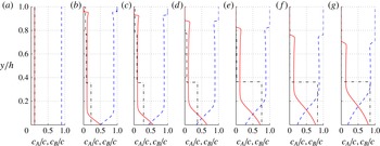
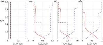
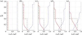
Predicted evolution with distance of the relative concentration profiles of large spheres (dashed blue lines) and small spheres (solid red lines) at seven different locations between the origin and the point at which the asymptotic solution is established: (a)
 $x/h=0$
, (b)
 $x/h=3$
, (c)
 $x/h=7$
, (d)
 $x/h=13$
, (e)
 $x/h=23$
, (f)
 $x/h=37$
, (g)
 $x/h=50$
. The simulation parameters are
 ${\it\phi}=26^{\circ }$
,
 $e=0.7$
,
 $r_{A}/r_{B}=1.7$
,
 $m_{A}/m_{B}=(1.7)^{3}$
,
 $V_{A}/V=0.9$
and
 $h/r_{AB}=11.8$
. The profile of the relative concentration of small spheres in the experiments of Savage & Lun (Reference Savage and Lun1988) (black dash-dotted line) is given for comparison. The vertical axes are the same in all figures.

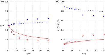
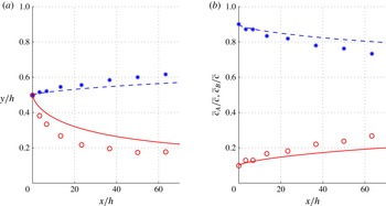
Predicted evolution with distance of (a) the COMs and (b) the depth-averaged relative concentrations of large spheres (dashed blue) and small spheres (solid red). The simulation parameters are the same as in figure 4. The experimental results of Savage & Lun (Reference Savage and Lun1988) for the large (blue stars) and small (red circles) spheres are given for comparison.

In figure 4 we show a comparison between the experimental results of Savage & Lun (Reference Savage and Lun1988) and the prediction of the theory for the case of a 10 % initial concentration of fine particles,
 $V_{A}/V=0.9$
, an angle of inclination of
 ${\it\phi}=26^{\circ }$
and a flow depth of 15 mm. Considering the experimental technique adopted to measure the segregation, based on a limited number of splitter plates and bins, the agreement is good, both in terms of the shapes of the concentration profiles and in terms of the longitudinal distance needed in order to reach the fully developed state. In particular, in figure 5 we show the evolution of the positions of the COMs of the large and small spheres with longitudinal distance and that of the depth-averaged concentrations of the two species. As already mentioned, the change of the relative depth-averaged concentration of the two species in the longitudinal direction is a consequence of the variation of the mixture velocity across the flow.
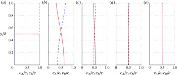
Predicted evolution with distance of the relative concentration profiles of large spheres (dashed blue lines) and small spheres (solid red lines) at four different locations between the origin and the point at which the asymptotic solution is established: (a)
 $x/h=0$
, (b)
 $x/h=5$
, (c)
 $x/h=10$
, (d)
 $x/h=20$
. The simulation parameters are
 ${\it\phi}=26^{\circ }$
,
 $e=0.7$
,
 $r_{A}/r_{B}=1.7$
,
 $m_{A}/m_{B}=(1.7)^{3}$
,
 $V_{A}/V=0.9$
and
 $h/r_{AB}=7.8$
. The profile of the relative concentration of small spheres in the experiments of Savage & Lun (Reference Savage and Lun1988) (black dash-dotted line) is given for comparison. The vertical axes are the same in all figures.

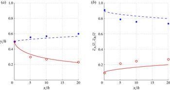
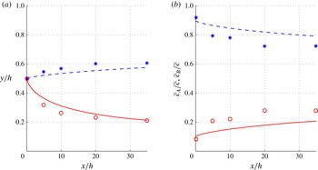
Predicted evolution with distance of (a) the COMs and (b) the depth-averaged relative concentrations of large spheres (dashed blue) and small spheres (solid red). The simulation parameters are the same as those in figure 6. The experimental results of Savage & Lun (Reference Savage and Lun1988) for the large (blue stars) and small (red circles) spheres are given for comparison.

Good agreement between experimental measurement and theoretical predictions is obtained also for a flow depth of 10 mm, when all of the other parameters are kept constant. In this case, the fully developed segregation is obtained at a distance that is less than the half of that needed for the thicker flow of the previous case, as shown in figures 6 and 7.
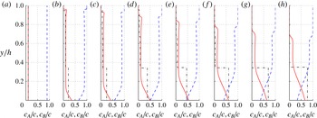
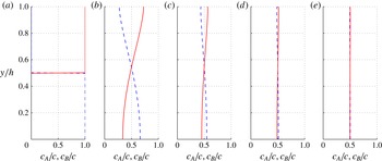
In figures 8–11, we present similar comparisons, but for a channel with a steeper slope. In this case, we also observe a slower segregation for the thicker flow. Moreover, we observe that the segregation also becomes slower if the slope is increased, in good agreement with experimental data. The increased advection due to the larger slope appears to have a more significant influence on the segregation distance than the increase in particle agitation.
Predicted evolution with distance of the relative concentration profiles of large spheres (dashed blue lines) and small spheres (solid red lines) at eight different locations between the origin and the point at which the asymptotic solution is established: (a)
 $x/h=0$
, (b)
 $x/h=3$
, (c)
 $x/h=7$
, (d)
 $x/h=13$
, (e)
 $x/h=23$
, (f)
 $x/h=37$
, (g)
 $x/h=50$
, (h)
 $x/h=63$
. The simulation parameters are
 ${\it\phi}=28^{\circ }$
,
 $e=0.7$
,
 $r_{A}/r_{B}=1.7$
,
 $m_{A}/m_{B}=(1.7)^{3}$
,
 $V_{A}/V=0.9$
and
 $h/r_{AB}=11.8$
. The profile of the relative concentration of small spheres in the experiments of Savage & Lun (Reference Savage and Lun1988) (black dash-dotted line) is given for comparison. The vertical axes are the same in all figures.

Predicted evolution with distance of (a) the COMs and (b) the depth-averaged relative concentrations of large spheres (dashed blue) and small spheres (solid red). The simulation parameters are the same as those in figure 8. The experimental results of Savage & Lun (Reference Savage and Lun1988) for the large (blue stars) and small (red circles) spheres are given for comparison.

Predicted evolution with distance of the relative concentration profiles of large spheres (dashed blue lines) and small spheres (solid red lines) at five different locations between the origin and the point at which the asymptotic solution is established: (a)
 $x/h=0$
, (b)
 $x/h=5$
, (c)
 $x/h=10$
, (d)
 $x/h=20$
, (e)
 $x/h=35$
. The simulation parameters are
 ${\it\phi}=28^{\circ }$
,
 $e=0.7$
,
 $r_{A}/r_{B}=1.7$
,
 $m_{A}/m_{B}=(1.7)^{3}$
,
 $V_{A}/V=0.9$
and
 $h/r_{AB}=7.8$
. The profile of the relative concentration of small spheres in the experiments of Savage & Lun (Reference Savage and Lun1988) (black dash-dotted line) is given for comparison. The vertical axes are the same in all figures.

Predicted evolution with distance of (a) the COMs and (b) the depth-averaged relative concentrations of large spheres (dashed blue) and small spheres (solid red). The simulation parameters are the same as those in figure 10. The experimental results of Savage & Lun (Reference Savage and Lun1988) for the large (blue stars) and small (red circles) spheres are given for comparison.

We obtain similar agreement with the results of the experiments of Savage & Lun (Reference Savage and Lun1988) when the relative volume of small particles is slightly increased, so
 $V_{A}/V_{B}=0.85$
. In this case, the observation that the segregation distance is shorter when the smaller species is more dilute is confirmed by the theory.
For given spheres and chute, the extended kinetic theory associates a unique volume flow rate to each flow depth (Jenkins & Berzi Reference Jenkins and Berzi2010). Consequently, the success of the theory in predicting the influence of depth on the evolution of segregation in the experiments of Savage & Lun (Reference Savage and Lun1988) is equivalent to success in predicting the influence of the inflow rate. That is, for larger flow depths, which are equivalent to larger inflow rates, the segregation evolution predicted by the theory is slower, as observed.
5. Two additional examples
5.1. Equal sizes, different masses
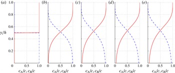
Up to this point, we have only analysed problems of size segregation of spheres made of the same material; in this case, the larger particles tend to rise (figure 12). However, the theory is also suitable for predicting profiles of relative concentration for binary mixtures of particles made of different materials. In particular, in agreement with what is shown by others (Drahun & Bridgwater Reference Drahun and Bridgwater1983; Alonso et al. Reference Alonso, Satoh and Miyanami1991; Jain et al. Reference Jain, Ottino and Lueptow2005a ,Reference Jain, Ottino and Lueptow b ; Larcher & Jenkins Reference Larcher and Jenkins2013) for spheres of the same size made of different materials, we predict that the heavier spheres stay down, while the lighter spheres stay up (figure 13).
Predicted profiles of the relative concentration of large spheres (dashed blue lines) and small spheres (solid red lines) for the radius ratio
 $r_{A}/r_{B}=1.0375$
and spheres made of the same material,
 $m_{A}/m_{B}=(r_{A}/r_{B})^{3}$
, at five equally spaced steps, each of 10 000 dimensionless time units (a–e). The simulation parameters are
 ${\it\phi}=25^{\circ }$
,
 $e=0.7$
,
 $V_{A}/V=0.5$
and
 $h/r_{AB}=20$
. The vertical axes are the same in all figures.

Predicted relative concentration profiles of heavy spheres (blue dashed lines) and light spheres (solid red lines) for spheres of the same size,
 $r_{A}/r_{B}=1$
, and a mass ratio of
 $m_{A}/m_{B}=2$
, at five equally spaced time steps, each of 4500 dimensionless time units (a–e). The simulation parameters are
 ${\it\phi}=25^{\circ }$
,
 $e=0.7$
,
 $V_{A}/V=0.5$
and
 $h/r_{AB}=20$
. The vertical axes are the same in all figures.

5.2. No segregation
Given the structure of (3.10) and (3.15) and the analogy with the steady segregation problem (Larcher & Jenkins Reference Larcher, Jenkins, Goddard, Jenkins and Giovine2010, Reference Larcher and Jenkins2013), we expect that mixtures of particles with particular size and mass ratios will exhibit perfect mixing. In the steady case, in order to have no gradient of
 $X$
normal to the bed and, therefore, no segregation, those terms in (4.3) that involve
 ${\it\delta}r$
and
 ${\it\delta}m$
must vanish. In figures 14 and 15, we show the evolution in time from an initial unmixed state to a final perfectly mixed state of the relative concentration profiles of a mixture of spheres for which this condition is valid, characterized by a radius ratio of
 $r_{A}/r_{B}=1.0375$
, also shown in figure 12 for spheres with the same material density, and a mass ratio of
 $m_{A}/m_{B}=2(r_{A}/r_{B})^{3}$
. The same density ratio was also shown in figure 13 for particles of the same size. The asymptotic solution is independent of the initial condition, which does affect the time needed to reach it. Four decimal places are retained in the specification of the radius ratio because of the extreme sensitivity of the mixing to the ratio.
As mentioned already for the steady theory (Larcher & Jenkins Reference Larcher and Jenkins2013), a necessary condition for no segregation is a uniform mixture concentration through the flow, a condition that is often observed, at least in first approximation, in dense gravity-driven granular flows with a free surface.
Predicted relative concentration profiles of the large heavy spheres (blue dashed lines) and small light spheres (solid red lines) for the radius ratio
 $r_{A}/r_{B}=1.0375$
and a mass ratio of
 $m_{A}/m_{B}=2(r_{A}/r_{B})^{3}$
, at five equally spaced time steps, from the initial state to the final perfectly mixed state, after 90 000 dimensionless time units (a–e). Initially, all of the large heavy spheres are in the lower half of the flow. The simulation parameters are
 ${\it\phi}=25^{\circ }$
,
 $e=0.7$
,
 $V_{A}/V=0.5$
and
 $h/r_{AB}=20$
. The vertical axes are the same in all figures.

Predicted relative concentration profiles of large heavy spheres (blue dashed lines) and small light spheres (red lines) for the radius ratio
 $r_{A}/r_{B}=1.0375$
and a mass ratio of
 $m_{A}/m_{B}=2(r_{A}/r_{B})^{3}$
, at five equally spaced time steps, from the initial state to the final perfectly mixed state, after 108 000 dimensionless time units (a–e). Initially, all of the small light spheres are in the lower half of the flow. The simulation parameters are
 ${\it\phi}=25^{\circ }$
,
 $e=0.7$
,
 $V_{A}/V=0.5$
and
 $h/r_{AB}=20$
. The vertical axes are the same in all figures.

Tunuguntla, Bokhove & Thornton (Reference Tunuguntla, Bokhove and Thornton2014) have carried out discrete numerical simulations to test for situations in which there is no segregation. However, the angle of inclination and the collision parameters that they employ do not result in a sufficiently dense flow for the extended kinetic theory to apply; see, for example, figure 4(b) of Silbert et al. (Reference Silbert, Ertas, Grest, Halsey, Levine and Plimpton2001). In such moderately dense flows, the mixture volume fraction varies through the entire depth of the flow; its variation, and that of the mixture temperature and mixture velocity, may be determined as a solution to a boundary value problem phrased using the classical kinetic theory (Arnarson & Jenkins Reference Arnarson, Jenkins, Helbing, Herrmann, Schreckenberg and Wolf2000).
Finally, we note that Jenkins & Yoon (Reference Jenkins and Yoon2002) considered segregation in an isothermal non-diffusive system subject to gravity, in which the large spheres were dilute in a dense gas of small spheres. The mechanism for segregation that was focused on there is often referred to as buoyancy, and the issue was the sign of the term
 $({\it\Gamma}_{2}{\it\delta}m+R_{2}{\it\delta}r)$
in (3.12). The system considered by Jenkins & Yoon (Reference Jenkins and Yoon2002) is different from the dense systems, sheared under gravity, of the present paper. In these, both diffusion and thermal segregation are present, and the volume fraction of large spheres is not, in general, small.
6. Conclusion
We have considered the evolution of particle segregation in collisional flows of two types of spheres down rigid bumpy inclines in the absence of sidewalls, in an analysis that was restricted to dense flows. An extension of kinetic theory was used to predict the concentration of the mixture and the profiles of mixture velocity and granular temperature. A kinetic theory for a binary mixture of nearly elastic spheres that do not differ by much in their size or mass was employed to predict the evolution of the concentration fractions of the two types of spheres. We treated situations in which the flow of the mixture was steady and uniform, but in which the segregation evolved, either in space or in time. The flow reaches uniformity before segregation evolves because the diffusion coefficient of (2.15) is proportional to
 $1/G$
, while the viscosity on which (2.25) is based is proportional to
 $G$
.
We applied the theory to situations in which there were data available from discrete numerical simulations and physical experiments. Employing reasonable values to characterize the particle interactions and no other adjustable parameters, we were able to reproduce both the qualitative features observed and the quantitative values measured in the simulation and experiments. In particular, and in accordance with measured data, we observed a slower segregation for thicker flows, when all the other parameters were kept constant. Moreover, we observed a slower evolution for steeper slopes and for similar volumes of the two species. The theory also shows that heavier spheres of the same size will sink and, for particular combinations of radius and mass ratios, segregation is inhibited and the flow evolves towards a perfect mixing of the two species.
The theory that we employed permits the understanding of how the rates of segregation with time and distance depend upon the depth of the flow relative to the average particle size, the angle of inclination of the flow, the coefficient of restitution and the total number or volume fraction of one species. The governing equations are based on the balances of mass, momentum and energy for the two species and the mixture. With respect to the predictions being sensitive to the properties of the particles and the governing equations being based on fundamental physical principals, our formulation differs from and improves upon existing phenomenological theories.
However, the theory has two quantitative deficiencies: it predicts sharper segregation profiles in the steady or asymptotic state than those observed in numerical simulations, and it predicts slower segregation than that measured. That is, it underestimates both diffusion and segregation rates. These deficiencies might be remedied by introducing appropriate numerical coefficients. We have resisted making such adjustments until it was clear what was predicted without them; however, it seems that making relatively small adjustments could improve upon the predictions.
Acknowledgements
The authors are grateful to the Department of Civil, Environmental and Mechanical Engineering at the University of Trento and to the School of Civil and Environmental Engineering at Cornell University for their financial support and hospitality. This research was supported in part by the National Science Foundation under grant no. NSF PHY11-25915 to the Kavli Institute of Theoretical Physics.
Appendix A
We assume that the radii and the masses of the two types of spheres do not differ by much and employ the characterizations
 ${\it\delta}r\equiv (r_{A}/r_{B})-1$
and
 ${\it\delta}m\equiv (m_{A}-m_{B})/m_{AB}$
of these differences.
Then, the gradient of the chemical potential and the thermal diffusion coefficient are given in terms of functions
 $G$
and
 $H$
related to the radial distribution function of a mixture, regarded as a single species with mass
 $m_{AB}/2$
and radius
 $r_{AB}/2$
:
 $$\begin{eqnarray}\frac{n}{T}\frac{\partial {\it\mu}_{A}}{\partial n_{A}}\,\doteq \,\frac{n}{n_{A}}+4G+4cH+24\frac{n_{B}}{n}cH{\it\delta}r\end{eqnarray}$$
and
 $$\begin{eqnarray}K_{T}^{(A)}\,\doteq \,\frac{5n_{A}n_{B}}{58n^{2}}\left[\left(2+\frac{c(3-c)}{2-c}-\frac{12}{5}G\right){\it\delta}r+\left(\frac{21}{2}+\frac{126}{5}G\right){\it\delta}m\right],\end{eqnarray}$$
where (Torquato Reference Torquato1995)
 $$\begin{eqnarray}G=5.69c\frac{c_{M}-0.49}{c_{M}-c}\end{eqnarray}$$
and
 $$\begin{eqnarray}H\equiv \frac{\text{d}G}{\text{d}{\it\nu}}=G\frac{c_{M}}{c(c_{M}-c)}.\end{eqnarray}$$
We introduce the measure of the segregation
 $$\begin{eqnarray}X=\frac{1}{2}\frac{n_{A}-n_{B}}{n}\end{eqnarray}$$
that arises naturally in the kinetic theory for segregation in binary mixtures of spheres (Arnarson & Jenkins Reference Arnarson and Jenkins2004). Then, to first order in the small quantities
 ${\it\delta}r$
and
 ${\it\delta}m$
,
 $$\begin{eqnarray}\displaystyle & \displaystyle \frac{{\it\rho}_{A}-{\it\rho}_{B}}{{\it\rho}}\,\doteq \,2X+2\left(1-4X^{2}\right){\it\delta}m, & \displaystyle\end{eqnarray}$$
 $$\begin{eqnarray}\displaystyle & \displaystyle \frac{{\it\rho}_{A}{\it\rho}_{B}}{{\it\rho}}\,\doteq \,\frac{m_{A}n}{4}(1-4X^{2})[1-(1+2X){\it\delta}m], & \displaystyle\end{eqnarray}$$
 $$\begin{eqnarray}\displaystyle & \displaystyle p_{A}\,\doteq \,n_{A}T\left[1+4G+2G\frac{n_{B}}{n}\left({\it\lambda}+3\right){\it\delta}r\right], & \displaystyle\end{eqnarray}$$
where
 ${\it\lambda}\equiv c(3-c)/(2-c)$
, and
 $$\begin{eqnarray}K_{AB}\,\doteq \,4G\frac{n_{A}n_{B}}{n}\left[1+\frac{1}{2}\left(\frac{n_{B}}{n}-\frac{n_{A}}{n}\right)\left({\it\lambda}+3\right){\it\delta}r\right].\end{eqnarray}$$
When these expressions are used in (2.8), we obtain
 $$\begin{eqnarray}\displaystyle \tilde{\boldsymbol{v}}_{A}-\tilde{\boldsymbol{v}}_{B} & = & \displaystyle -\frac{n^{2}}{n_{A}n_{B}}D_{AB}\left\{-\frac{{\it\rho}_{A}}{nT}\boldsymbol{g}\cos {\it\phi}\right.+\frac{n_{A}}{nT}\left[1+4G+2G\frac{n_{B}}{n}({\it\lambda}+3){\it\delta}r+4G\frac{n_{B}}{n}{\it\delta}m\right]\boldsymbol{{\rm\nabla}}T\nonumber\\ \displaystyle & & \displaystyle +\,\frac{n_{A}}{n^{2}}\left[\frac{n}{n_{A}}+4G+4cH+24\frac{n_{B}}{n}cH{\it\delta}r\right]{\rm\nabla}n_{A}+\frac{n_{A}}{n^{2}}[4G+4cH-24XcH{\it\delta}r]\boldsymbol{{\rm\nabla}}n_{B}\nonumber\\ \displaystyle & & \displaystyle \left.+\,\frac{1}{T}\frac{5n_{A}n_{B}}{58n^{2}}\left[\left(2+{\it\lambda}-\frac{12}{5}G\right){\it\delta}r+\left(\frac{21}{2}+\frac{126}{5}G\right){\it\delta}m\right]\boldsymbol{{\rm\nabla}}T\right\},\end{eqnarray}$$
in which the balance of force across the mixture,
 $\boldsymbol{{\rm\nabla}}P={\it\rho}\boldsymbol{g}\cos {\it\phi}$
, has been used to eliminate the gradient of the mixture pressure.
We next express the gradients of
 $n_{A}$
and
 $n_{B}$
in terms of
 $\boldsymbol{g}$
and the gradients of
 $c$
and
 $T$
. Using
 $n_{A}=(0.5+X)n$
,
 $n_{B}=(0.5-X)n$
and
 $n=6c(1-3X{\it\delta}r)/({\rm\pi}r_{AB}^{3})$
, we have
 $$\begin{eqnarray}\frac{n_{A}n_{B}}{n^{2}}=0.25-X^{2}\quad \text{and}\quad \frac{n_{A}}{n^{2}}=\frac{{\rm\pi}r_{AB}^{3}}{6c}\frac{0.5+X}{(1-3X{\it\delta}r)}=\frac{{\rm\pi}r_{AB}^{3}}{6c}(0.5+X)(1+3X{\it\delta}r);\end{eqnarray}$$
therefore,
 $$\begin{eqnarray}\boldsymbol{{\rm\nabla}}n_{A}=\frac{6}{{\rm\pi}r_{AB}^{3}}\{c[1-(1.5+6X){\it\delta}r]\boldsymbol{{\rm\nabla}}X+(0.5+X)(1-3X{\it\delta}r)\boldsymbol{{\rm\nabla}}c\}\end{eqnarray}$$
and
 $$\begin{eqnarray}\boldsymbol{{\rm\nabla}}n_{B}=-\frac{6}{{\rm\pi}r_{AB}^{3}}\{c[1+(1.5-6X){\it\delta}r]\boldsymbol{{\rm\nabla}}X-(0.5-X)(1-3X{\it\delta}r)\boldsymbol{{\rm\nabla}}c\}.\end{eqnarray}$$
Then,
 $$\begin{eqnarray}\displaystyle \tilde{\boldsymbol{v}}_{A}-\tilde{\boldsymbol{v}}_{B} & = & \displaystyle -\frac{1}{0.5-X}D_{AB}\left\{-\frac{1}{0.5+X}\frac{{\it\rho}_{A}}{nT}\boldsymbol{g}\cos {\it\phi}\right.+\left[\frac{1}{0.5+X}-3(1+4G){\it\delta}r\right]\boldsymbol{{\rm\nabla}}X\nonumber\\ \displaystyle & & \displaystyle +\left[(1+4G+4cH)+12(0.5-X)cH{\it\delta}r\right]\frac{\boldsymbol{{\rm\nabla}}c}{c}\nonumber\\ \displaystyle & & \displaystyle +\left(1+4G\right)\frac{\boldsymbol{{\rm\nabla}}T}{T}+\left(\frac{179}{58}G+\frac{105}{232}-\frac{179}{29}GX-\frac{105}{116}X\right){\it\delta}m\frac{\boldsymbol{{\rm\nabla}}T}{T}\nonumber\\ \displaystyle & & \displaystyle +\left.\left[G{\it\lambda}+\frac{168}{58}G+\frac{5}{58}+\frac{5}{116}{\it\lambda}-\left(2G{\it\lambda}+\frac{168}{29}G+\frac{5}{29}+\frac{5}{58}{\it\lambda}\right)X\right]{\it\delta}r\frac{\boldsymbol{{\rm\nabla}}T}{T}\right\}.\nonumber\\ \displaystyle & & \displaystyle\end{eqnarray}$$
The approximate expression for the pressure is
 $$\begin{eqnarray}P=m_{AB}\frac{3c}{{\rm\pi}r_{AB}^{3}}\left[1+2(1+e)G\right]w^{2}(1-3X{\it\delta}r),\end{eqnarray}$$
where
 $w^{2}\equiv 2T/m_{AB}$
. This, together with
 ${\it\rho}_{A}=m_{A}n_{A}$
,
 ${\it\rho}={\it\rho}_{A}+{\it\rho}_{B}$
,
 $c_{A}=4{\rm\pi}r_{A}^{3}n_{A}/3$
, and the approximations
 $m_{\text{A}}=m_{\text{AB}}(1+{\it\delta}m)/2$
,
 $m_{B}=m_{\text{AB}}(1-{\it\delta}m)/2$
and
 ${\it\rho}_{A}=m_{\text{AB}}(1+{\it\delta}m)(0.5+X)n/2$
can be used to write the gradient of
 $c$
in terms of
 $\boldsymbol{g}$
and the gradient in
 $T$
. The approximation to the gradient of the pressure is then
 $$\begin{eqnarray}\displaystyle \boldsymbol{{\rm\nabla}}P & = & \displaystyle \frac{6}{{\rm\pi}r_{AB}^{3}}(1-3X{\it\delta}r)\left[1+2(1+e)G\right]T\boldsymbol{{\rm\nabla}}c-\frac{18}{{\rm\pi}r_{AB}^{3}}c{\it\delta}r\left[1+2(1+e)G\right]T\boldsymbol{{\rm\nabla}}X\nonumber\\ \displaystyle & & \displaystyle +\,\frac{12(1+e)}{{\rm\pi}r_{AB}^{3}}(1-3X{\it\delta}r)cHT\boldsymbol{{\rm\nabla}}c+\frac{6}{{\rm\pi}r_{AB}^{3}}(1-3X{\it\delta}r)c\left[1+2(1+e)G\right]\boldsymbol{{\rm\nabla}}T.\qquad \quad\end{eqnarray}$$
Using this with the balance of force across the mixture,
 $$\begin{eqnarray}\boldsymbol{{\rm\nabla}}P={\it\rho}\boldsymbol{g}\cos {\it\phi}=-\frac{m_{AB}}{2}(1+2X{\it\delta}m)\frac{6}{{\rm\pi}r_{AB}^{3}}c(1-3X{\it\delta}r)\boldsymbol{g}\cos {\it\phi},\end{eqnarray}$$
gives
 $$\begin{eqnarray}\displaystyle & & \displaystyle \left[1+2(1+e)(G+cH)\right](1-3X{\it\delta}r)\frac{\boldsymbol{{\rm\nabla}}c}{c}-3\left[1+2(1+e)G\right]{\it\delta}r\boldsymbol{{\rm\nabla}}X\nonumber\\ \displaystyle & & \displaystyle \qquad +\,(1-3X{\it\delta}r)\left[1+2(1+e)G\right]\frac{\boldsymbol{{\rm\nabla}}T}{T}\nonumber\\ \displaystyle & & \displaystyle \quad =\frac{m_{AB}}{2}(1+2X{\it\delta}m)(1-3X{\it\delta}r)\frac{\boldsymbol{g}\cos {\it\phi}}{T}.\end{eqnarray}$$
Therefore, finally, (A 14) may be written as
 $$\begin{eqnarray}\displaystyle \tilde{\boldsymbol{v}}_{A}-\tilde{\boldsymbol{v}}_{B}=-D_{AB}\left\{({\it\Gamma}_{1}{\it\delta}m+R_{1}{\it\delta}r)\frac{\boldsymbol{{\rm\nabla}}T}{T}\hspace{-2.0pt}-\hspace{-2.0pt}({\it\Gamma}_{2}{\it\delta}m+R_{2}{\it\delta}r)\frac{m_{AB}\boldsymbol{g}\cos {\it\phi}}{2T}\hspace{-2.0pt}+\hspace{-2.0pt}\frac{\boldsymbol{{\rm\nabla}}X}{0.25-X^{2}}\right\}\!,\qquad & & \displaystyle\end{eqnarray}$$
where
 $$\begin{eqnarray}\displaystyle & {\it\Gamma}_{1}=\displaystyle \frac{179}{29}G+\displaystyle \frac{105}{116}, & \displaystyle\end{eqnarray}$$
 $$\begin{eqnarray}\displaystyle & \displaystyle R_{1}=\frac{5}{58}\left[2+\frac{c(3-c)}{2-c}-\frac{12}{5}G\right]+2G\left[3+\frac{c(3-c)}{2-c}\right]-\frac{12cH(1+4G)}{1+4G+4cH}, & \displaystyle\end{eqnarray}$$
with
 $$\begin{eqnarray}H=\frac{c_{M}G}{c(c_{M}-c)}\end{eqnarray}$$
and
 $$\begin{eqnarray}{\it\Gamma}_{2}=2\quad \text{and}\quad R_{2}=-\frac{12cH}{1+4G+4cH}.\end{eqnarray}$$