

1 Introduction
As agent-based modeling (ABM) has been increasingly applied to the study of social phenomena, there has been more empirical approaches than ever. During early days of ABM, exploratory attempts were extremely abstract with rich interpretations. It may be useful to make a list, which will surely become very lengthy, of the application of the Ising model, for instance, to various types of phenomena over recent decades (McCoy and Wu Reference McCoy and Wu2014). Without doubt, a simple model may be applicable to, and able to explain, a large number of phenomena that seem unrelated to one another. The making of simple models was not only advised but also accepted in order to extract the essence of various research activities. The most famous maxim in the field must be KISS (‘Keep It Simple, Stupid’) that was first introduced by Robert Axelrod (Reference Axelrod1997a: 4–5) to the field.
The current trend of ABM looks at a departure from the KISS principle. As such, KISS may be replaced by ‘TASS’, which stands for ‘Time And Space Specified’. In either theory-oriented or history-oriented studies, the empirical approach requires some kind of empirical data that specifically represent a certain point or range of both time and space. In this sense, the introduction of empirical data into ABM may be characterized as TASS modeling.
This article aims to demonstrate the promising possibilities of the change of emphasis from KISS to TASS in ABM applications in social sciences. Namely, this article adopts the empirical approach employing ABM that used to be built based on KISS. Although the ways to specify time and space are numerous, this article focuses on the spatial dimension and attempts to analyze a KISS model with geographical data that are constructed from geographic information systems (GIS). While spatial analysis is widely attempted in ABM, because of the common setting of interaction among agents on a two-dimensional plane, it is difficult (actually time-consuming and tedious) at best to import spatial data into the computational model, even if such data are available from GIS. Some tools that incorporate ABM with spatial data are needed in order to build a TASS agent-based model. As for the tool for ABM, it is customary for the authors to use the ABM-specific simulator named artisoc developed by the Kozo Keikaku Engineering (KKE). Recently, KKE developed the GIS data converter for artisoc, which converts various types of spatial data into the spatial variables compatible with artisoc, which allows for automatic data transformation and easier use of spatial data in ABM. The empirical analyses in this article are made possible thanks to it.Footnote 1
The KISS model that is used here is the segregation model developed by Thomas Schelling nearly half a century ago (Schelling, Reference Schelling1969, Reference Sakoda1971, Reference Schelling1978). A pioneering and monumental attempt at ABM, the model is so well-known that it must be unnecessary to describe it here (see Clark and Fossett, Reference Clark and Fossett2008; Hatna and Benenson, Reference Hatna and Benenson2014; Vinkovic and Kirman, Reference Vinkovic and Kirman2006, for extensive reviews). Because the spatial structure of the segregation model is so simple that only the neighborhood is defined, it may be necessary to add some spatial variables in order to apply the model to the empirical analysis. The element of TASS in this article is geo-referenced (spatial) census data of the metropolitan Chicago area. Because Chicago is one of the cities in which residential segregation is clearly observed, it is an appropriate case to explicitly incorporate the KISS-type Schelling's segregation model with empirical data. Although analyses in this article are preliminary, they hopefully demonstrate the promising possibility of TASS modeling.
In the next section, existing applications of the ABM technique and their empirical turn are surveyed. Then, the classic Schelling's model of residential segregation is incorporated with newly available fine-grained demographic data to demonstrate the methodological utility of the TASS-type ABM. Preliminary analyses is followed by discussion and conclusions concerning the application of this empirically explicit computational modeling approach to social sciences.
2 From the KISS to the TASS principle
The micro–macro link, or the relationship between individual behavior at the micro level and collective outcomes at the macro level sits at the center of numerous scholarly debates in social science (Coleman, Reference Coleman1990). Theories of social science are often considered to be more informative if they account for how and why individual actions and interactions add up to collective behavior, or the causal mechanisms/relationships between ‘micromotives’ and ‘macrobehavior’ (Bruch and Mare, Reference Bruch and Mare2006: 667–668). As Schelling (Reference Schelling1978) argues:
Sometimes they are not easily guessed. Sometimes the analysis is difficult. Sometimes it is inconclusive. But even inconclusive analysis can warn against jumping to conclusions about individual intentions from observations of aggregates, or jumping to conclusions about the behavior of aggregates from what one knows or can guess about individual intentions. (p. 14)
Agent-based modeling (ABM) has been used to simulate and specify the relationship between autonomous actions and interactions of individuals and the dynamics and behavior of the whole system. Cederman (Reference Cederman2005: 873) defines ABM as a ‘computational methodology that allows scientists to create, analyze, and experiment with artificial worlds populated by agents that interact in nontrivial ways and that constitute their own environment’. In ABM, researchers code the actions and interactions of constituent elements of a system, called agents, into a program and examine what systemic or collective outcomes emerge through computational simulations. As such, ABM enables us to systematically explore whether, how, and why some specific micro-level mechanisms generate a class of macro-level outcomes not reducible to properties of the constituent agents (Axelrod, Reference Axelrod1997a; Cederman, Reference Cederman2005; Epstein and Axtell, Reference Epstein and Axtell1996; Macy and Willer, Reference Macy and Willer2002).
2.1 Agent-based modeling and the KISS principle
A model serves as a purified experiment, and ABM technique provides a ‘computer laboratory for virtual experimentation’ (Crooks et al., Reference Crooks2008: 418). Among the pioneering works, Axelrod (Reference Axelrod1997a: 4–5) argues:
Although agent-based modeling employs simulation, it does not necessarily aim to provide an accurate representation of a particular empirical application. Instead, the goal of agent-based modeling is to enrich our understanding of fundamental processes that may appear in a variety of applications. This requires adhering to the KISS principle, which stands for the army slogan ‘keep it simple, stupid’.
Most existing ABM applications adhere to the KISS principle and have specified the micro-mechanisms sufficient to generate macro-outcomes such as residential segregation, evolution of cooperation in the multi-player Iterated Prisoners Dilemma game, and dissemination of culture (Axelrod, Reference Axelrod1984, Reference Axelrod1997a, Reference Axelrodb; Schelling, Reference Schelling1969, Reference Sakoda1971, Reference Schelling1978). In a sense, the concepts of ABM in social science date back to the 1970s, and a pioneering contribution must be the work of Thomas Schelling (Reference Schelling1969, Reference Sakoda1971, Reference Schelling1978) who developed a model of residential segregation by moving pennies and dimes on a chessboard. Assuming that coins represent householders of different race seeking to reside amongst one's own kind, he demonstrated that marked segregation within neighborhoods could emerge from seemingly mild, not strong, individual preferences (see Sakoda, Reference Sakoda1971, for similar games). Having yielded the counterintuitive insight, Schelling's parsimonious model is now regarded as a ‘theoretical basis’ for the scholarly debate on the causes of residential segregation (Clark and Fossett, Reference Clark and Fossett2008: 4109).
The last few decades have witnessed an explosion of ABM applications. Political scientists and sociologists have examined and extended existing theories through ABM (e.g., Axelrod, Reference Axelrod1997a; Bhavnani et al., Reference Bhavnani, Findley and Kuklinski2009; Bremer and Mihalka, Reference Bremer, Mihalka, Deutsch, Fritsch, Jaguaribe and Markovits1977; Cederman, Reference Cederman1997, Reference Cederman2002, Reference Cederman2005; Cusack and Stoll, Reference Cusack and Stoll1990; Johnson et al., Reference Johnson, Weidmann and Cederman2011; Laver and Sergenti, Reference Laver and Sergenti2012; Lustick et al., Reference Lustick, Miodownik and Eidelson2004; Schrodt, Reference Schrodt1981; Siegel, Reference Siegel2009, Reference Siegel2011). Physicists have developed agent-based models to analyze social phenomena (see Castellano et al., Reference Castellano, Fortunato and Loreto2009; Helbing et al., Reference Helbing, Brockmann, Chadefaux, Donnay, Woolley-Meza, Moussaid, Johansson, Krause, Schutte and Perc2015, for comprehensive reviews). Because of the increasing number of modeling attempts, there is now more confidence that ABM is a ‘valid technical methodology’ for scientific inquiry (Janssen and Ostrom, Reference Helbing, Brockmann, Chadefaux, Donnay, Woolley-Meza, Moussaid, Johansson, Krause, Schutte and Perc2006).
2.2 Time and space specified (TASS) modeling
The KISS principle stresses simplicity rather than realism. Adhering to the KISS principle, most conventional ABM applications remain abstract and are rarely tested against empirical data (Janssen and Ostrom, Reference Janssen and Ostrom2006; Lustick and Miodownik, Reference Lustick and Miodownik2009). However, overly abstract models may lead to arbitrary interpretations and thus bring into question the appropriateness of ABM in explaining known empirical phenomena. For example, Axelrod (Reference Axelrod1997b) uses the simulation outcomes of a single agent-based model named dissemination of culture to explain various phenomena at different analytical levels such as the process of national integration, the survival of a heterogeneous minority surrounded by overwhelming majority, and regional integration seen in Europe. Researchers skeptical of ABM often acutely criticize this problem (Mitsutsuji and Yamakage, Reference Mitsutsuji and Yamakage2013). While parsimony is vital in modeling attempts, models must also have explicit connections with empirical observations to enrich our understanding of generating processes underlying social phenomena and address such criticism. Otherwise, it may be extremely difficult to test, evaluate, or validate agent-based models using empirical data. Consequently, a natural question emerges: Whether and to what extent can the model predictions explain empirical phenomena?
Such a speculation leads to the idea of incorporating agent-based models with empirical data to tighten the connections between models and empirical phenomena, or to make models time and space specified (TASS). Rather than yielding purely theoretical insights, TASS modeling may identify micro-mechanisms sufficient to generate macro-outcomes consistent with observed ones. While no computational models can perfectly ‘re-run’ history, such models can serve as heuristic devices that enhance our understanding of generating processes underlying empirical phenomena (Janssen and Ostrom, Reference Janssen and Ostrom2006; Lustick and Miodownik, Reference Lustick and Miodownik2009; Weidmann and Salehyan, Reference Weidmann and Salehyan2013).
Although the ways to specify time and space are numerous, increasingly available spatial data and the recent developments of geographic information systems (GIS) provide an opportunity to tighten the connection between purified models and empirical phenomena through the use of geo-referenced empirical data (Crooks et al., Reference Crooks, Castle and Batty2008; Lustick and Miodownik, Reference Lustick and Miodownik2009; O'Sullivan, Reference O'Sullivan2008; Torrens and Benenson, Reference Torrens and Benenson2005). Indeed, some researchers have started to use increasingly available spatial data to test, evaluate, and validate their models with empirical observations and thereby have moved beyond the KISS principle. Initial contributions by sociologists include models that incorporate Schelling's segregation model with geo-referenced demographic and dwelling price data (e.g., Benenson et al., Reference Benenson, Omer and Hatna2002, Reference Benenson, Hatna and Or2009; Bruch, Reference Bruch2014; Crooks, Reference Crooks2008; Yin, Reference Yin2009). For example, Benenson et al. (Reference Benenson, Omer and Hatna2002, Reference Benenson, Hatna and Or2009) and Yin (Reference Yin2009) show that modified or generalized versions of Schelling's segregation model were applicable to and explainable of segregation patterns observed in real cities using detailed spatial data on the Tel Aviv and Buffalo metropolitan areas respectively. These results illustrate that that observed patterns of residential segregation could plausibly arise from mild racial and economic preferences.
Political scientists and physicists have also developed another class of TASS models to examine the determinants of violence in civil war (e.g., Bhavnani and Choi, Reference Bhavnani and Choi2012; Bhavnani et al., Reference Bhavnani, Miodownik and Choi2011, Reference Bhavnani, Donnay, Miodownik, Mor and Helbing2014; Lim et al., Reference Lim, Metzler and Bar-Yam2007; Sakamoto, Reference Sakamoto2013; Weidmann and Salehyan, Reference Weidmann and Salehyan2013). Lim et al. (Reference Lim, Metzler and Bar-Yam2007) and Weidmann and Salehyan (Reference Weidmann and Salehyan2013) propose agent-based models similar to Schelling's model incorporating detailed spatial data of ethnic geography and analyzing the patterns of violence and segregation in the former Yugoslavia and in Iraq. They demonstrate that a simple mechanism of ethnically and/or security motivated migration and subsequent violence accounts for the spatial distributions of violence in actual conflicts and successfully predicts them. Such empirically plausible models could also serve as heuristic devices to explore the possible effects of proposed policy efforts. Having optimized model parameters such that the patterns of violence from the simulation closely fit the actual distributions, Bhavnani et al. (Reference Bhavnani, Donnay, Miodownik, Mor and Helbing2014) use an agent-based model to assess how different levels of Israeli–Palestinian segregation would shape future violence in Jerusalem.
These modeling attempts have successfully specified the micro-mechanisms sufficient to generate empirically observed macro-outcomes and demonstrated that empirically grounded agent-based models are extremely useful in identifying and testing causal mechanism. Incorporating agent-based models with spatial data seems to be a promising way to go beyond the KISS principle toward the TASS principle.
3 A working example: applying Schelling's model of segregation to Chicago
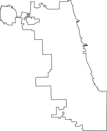
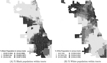
This section provides a working example of TASS modeling incorporating Schelling's (Reference Schelling1969, Reference Schelling1971, Reference Schelling1978) classic model of segregation with geo-referenced demographic data on Chicago derived from the US Census 2010. The city of Chicago is not only one of the most diverse cities, but also one of the most racially segregated cities in the United States. Figures 1 and 2 represent the city boundary and the population distribution among the 2010 Census tracts of Chicago, respectively. As Charles (Reference Charles2003) and Logan et al. (Reference Logan, Stults, Board, Anderson, Bianchi, Bluestone, Danziger, Fischer, Lichter and Prewitt2011) argue, many of the large and ethnically diverse US cities remain highly, though not completely, segregated. Chicago contains not only highly homogeneous segregated clusters but also heterogeneous integrated mosaics as shown in Figure 2.
City-level administrative boundary of Chicago

Spatial distribution of Black/White population in Chicago Notes: Data are derived from the US Census 2010. Note that the outer limit of census tracts is slightly different from the city-level administration boundary (Figure 1). Darker shade represents a higher proportion of Black/White population (P0030002/P0030003) over the total population (P0030001) within the tract, and solid lines represent census tract boundaries. Census tracts containing NAs for any of total (P0030001), White (P0030002), or Black population (P0030003) are dropped.

One might think that individual residents must have strong racial preferences for this segregation pattern to emerge. However, this intuition does not always hold. Survey evidence suggests that while individuals do favor residing with neighbors of the same race, such preferences are rather modest (e.g., Bruch and Mare, Reference Bruch and Mare2006; Clark, Reference Clark1991; Clark and Fossett, Reference Clark and Fossett2008; Emerson et al., Reference Emerson, Yancey and Chai2001; Farley et al., Reference Farley, Schuman, Bianchi, Colasanto and Hatchett1978; Krysan et al., Reference Krysan, Couper, Farley and Forman2009; Xie and Zhou, Reference Xie and Zhou2012). This is a gap in search of a theory. As discussed in detail below, Schelling's segregation model provides a possible explanation to this seemingly puzzling phenomenon.Footnote 2
3.1 Technical challenges
While the recent empirical turn in ABM is a welcome trend, it currently takes in-depth ABM and GIS skills to be able to exploit opportunities offered by TASS modeling. Nonetheless, the recent developments in software provide a solution to this technical challenge, at least partly. Our model is written in artisoc, a user-friendly agent-based toolkit developed by the Kozo Keikaku Enterprise (KKE). The KKE GIS data converter for artisoc is used to couple our agent-based model with spatial data on Chicago. The software allows for easier building of agent-based models and handling of spatial data in ABM. In the current context, high-resolution geo-referenced demographic data provided by the US Census 2010 are extremely useful and freely available from the US National Historical Geographic Information System (NHGIS, https://www.nhgis.org/). While combining and converting spatial data may be another technical challenge, a series of open-source packages named UScensus-suite (Almquist, Reference Almquist2010) for R allows for convenient handling of the US Census data. As R is one of the most popular statistical software packages among students of social science, Almquist (Reference Almquist2010) is a welcome addition to the spatial econometrics/statistics packages released on CRAN (http://cran.r-project.org/; see Bivand et al., Reference Bivand, Pebesma and Gómez-Rubio2013 and CRAN Task View: Analysis of Spatial Data at http://cran.r-project.org/web/views/Spatial.html, for further details). Our empirical data are derived from the US Census 2010 and handled using R and GIS data converter for artisoc.
Offering a comprehensive explanation for residential segregation in Chicago is beyond the scope of this article. Instead, we aim to demonstrate how TASS modeling helps to tighten the connection between theoretical models and empirical phenomena and allows for easier empirical evaluation of models. We present a working example in the following way. First, we replicate Schelling's segregation model using a hypothetical square lattice and examine simulation outcomes. Second, we replace the hypothetical lattice with more a specified one representing the 2010 Census tracts within the Chicago city boundary. This modification enables us to explore whether and how well the classic segregation model is able to generate spatial segregation patterns consistent with the observed one as Schelling (Reference Schelling1969: 488) himself once implied.
3.2 Replicating Schelling's model of segregation
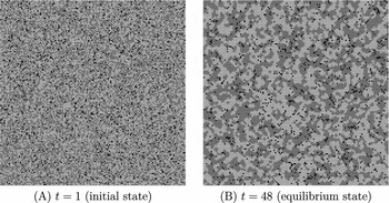
Schelling's (Reference Schelling1969, Reference Schelling1971, Reference Schelling1978) model considers spatial distribution of racial groups as an outcome of repeated interactions between individual householders. Our baseline agent-based model replicates the original model on a two-dimensional 150 × 150 square lattice; that is, a grid with 225,000 cells as shown in Figure 3(A). The lattice is populated with ‘penny’ (dark gray) and ‘dime’ (light gray) agents that represent householders of different racial groups. A small proportion of grid-cells are left unpopulated. Each agent can occupy one grid-cell, or a ‘housing unit’, at a discrete moment of time step and move to another unpopulated cell when she/he is not satisfied with the current position. Because agents are assumed to have mild preferences for living amongst like agents, their decisions whether or not to move to another cell depend on the number of like and unlike agents among neighborhoods.
Schelling's model of segregation on a two-dimensional 150 × 150 lattice Notes: Panel (A) shows the initial spatial configuration of ‘penny’ and ‘dime’ agents. The lattice becomes highly segregated at time step 48 as panel (B) shows. Dark gray and light gray cells represent penny and dime agents respectively. Black cells are currently unoccupied (π = 0.95).

To describe the model more formally, let Ag denote the set of agents belonging to one of two mutually avoiding groups g ∈ {penny, dime}. Each agent Agi ∈ Ag is randomly placed on a different cell at the beginning of a simulation run. A model parameter π determines the proportion of populated cells. Once the lattice has been populated with agents, the model proceeds in a series of time steps t.
For simplicity, we assume that (1) there are 50% penny and 50% dime agents on the lattice, (2) the number of agents is held for the entire model period, (3) preferences of agents are held for the entire model period, (4) agents’ groups are observable and thus Agi can perfectly distinguish neighbor agents belonging to g from those not belonging to g, and (5) agents possess knowledge about all the neighbors surrounding every agent.Footnote 3 Following Benenson et al. (Reference Benenson, Hatna and Or2009, 468–470), the agents' behavior algorithm is defined as follows:
(1) At every time step t, each agent Agi belonging to a group g observes the set of neighborhood cells
 ${\cal N}_{\rm j}$ around the currently located cell j and computes the fraction sjt of the cells occupied by agents belonging to g among ${\cal N}_{\rm j}$.Footnote 4
(2) If sjt < predetermined threshold (common racial preference) θ, then Agi decides to relocate; otherwise, it decides to stay.
(3) If Agi decides to relocate, it randomly chooses a currently unoccupied cell k and runs rule (1) to compute skt.
(4) If skt > sjt, Agi moves to cell k; otherwise, it stays.
(5) Previously occupied cell j becomes unoccupied and available to other agents.

Once all agents have executed the behavior rule, time step count increases to t + 1. A simulation run continues until the spatial distribution of agents reaches either (1) an equilibrium where all agents are satisfied with their current locations or (2) a dynamic equilibrium where agents may still be dissatisfied and moving but the composition of neighborhoods is no longer changing, or (3) time step count t reaches to T. We set T = 10, 000 and the proportion of populated cells π = 0.95 for the following simulation runs. The above representation is slightly modified and generalized compared with the original model (Benenson et al., Reference Benenson, Hatna and Or2009: 468–70). The original model assumes that preference threshold θ = 1/3 and the size and the form of local neighborhoods each agent cares about  ${\cal N}$ is a 3 × 3 Moore neighborhood (eight nearest cells). While further generalization or modification is possible, it is known that simulation outcomes critically depend on these two parameters (e.g., Bruch and Mare, Reference Bruch and Mare2006; Clark and Fossett, Reference Clark and Fossett2008; Crooks, Reference Crooks2008; Hatna and Benenson, Reference Hatna and Benenson2014; Laurie and Jaggi, Reference Laurie and Jaggi2003; Vinkovic and Kirman, Reference Vinkovic and Kirman2006). Note that the baseline value of θ is quite small, meaning that both penny and dime agents have mild preferences and thus tolerate a large proportion of unlike neighbors among their neighborhoods.
Figure 3 (B) shows a typical simulation outcome with θ and ${\cal N}$ set as above. The figure illustrates that a highly segregated pattern at the macro-level, a phenomenon not directly foreseen from the individual motives, could emerge from mild segregation preferences at the micro-level (Schelling, Reference Schelling1978; 148–55). Fraction sjt defined in rule (1) serves as a measure of segregation for a given agent at time step t, and the measure of global segregation level at t, St, can be given by calculating the mean fraction value. Because agents are randomly placed at the beginning of a simulation run, the initial segregation level S 1 roughly equals 0.5. In the illustrative run shown in Figure 3, S 48 increases to 0.763 at time step 48 when all agents are satisfied, suggesting that mild individual preferences to segregate are sufficient for global segregation.
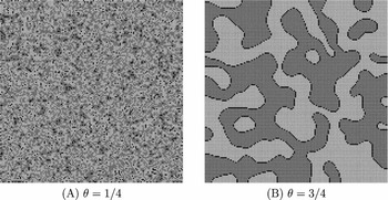
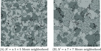
In Figures 4 and 5, we vary two main model parameters, the preference threshold θ and the definition of neighborhoods ${\cal N}$, to explore whether and how agents’ segregation preferences and neighborhood scopes influence the spatial patterns of segregation. Three results emerge. First, as easily expected, the square-lattice becomes more segregated as θ increases, meaning that stronger segregation preferences at the micro level lead to higher segregation at the macro level as shown in Figure 4.Footnote 5 Second, the resulting segregation level is not very sensitive to the definition of ${\cal N}$. The global segregation level at time step T, ST, remains 0.761 and 0.729 for panels (A) and (B) of Figure 5 respectively. Table 1 reports the mean resulting segregation level⟨ST⟩ over 300 replications for each parameter setting with different random seeds, which confirms that the results shown in Figure 5 are not accidental.Footnote 6 Finally and qualitatively, as the size of ${\cal N}$ increases so do the sizes of homogeneous clusters (of agents belonging to the same group) and heterogeneous areas. While a simulation run with a small ${\cal N}$ converges to segregation in a long run (Figures 3 and 4), a simulation run with a greater ${\cal N}$ yields a mixed spatial pattern that contains both segregated patches for each group as well as integrated patches where both groups coexist (Figure 5).Footnote 7
Representative cases with different values of racial preference threshold θ Notes: Panel (A) shows a typical simulation outcome with highly tolerant agents and panel (B) represents another outcome with highly intolerant agents. A greater θ means a stronger preference for neighbors of the same kind. The two panels demonstrate that both resulting segregation level and the sizes of homogeneous clusters are positively correlated with preference threshold θ.

Representative cases with different sizes of neighborhoods, ${\cal N}$Notes: Two panels show typical simulation outcomes with ${\cal N}$ a 5 × 5 Moore neighborhood (24 nearest cells) and ${\cal N}$ = a 7 × 7 Moore neighborhood (48 nearest cells) respectively, with θ = 1/3. The number of neighborhood cells agents observe increases as the size ${\cal N}$ increases. The sizes of both homogeneous (segregated) clusters and heterogeneous (integrated) mosaics increase as the size of ${\cal N}$ increases

300 replications of simulation runs for each parameter setting

Note: Standard deviations in parentheses.
aBaseline setting.
These results suggest that the levels of segregation mainly depends on the preference threshold θ while the forms of segregation is highly sensitive to the neighborhood definition ${\cal N}$.Footnote 8 Because real cities are rarely completely segregated but rather exhibit mixed patterns that consist of both homogeneous clusters and heterogeneous mosaics, the simple exercise indicates that a segregation model with a greater ${\cal N}$ is likely to be a better heuristic tool to enrich our understanding of empirical phenomena than the original model.
3.3 Incorporating the segregation model with spatial data
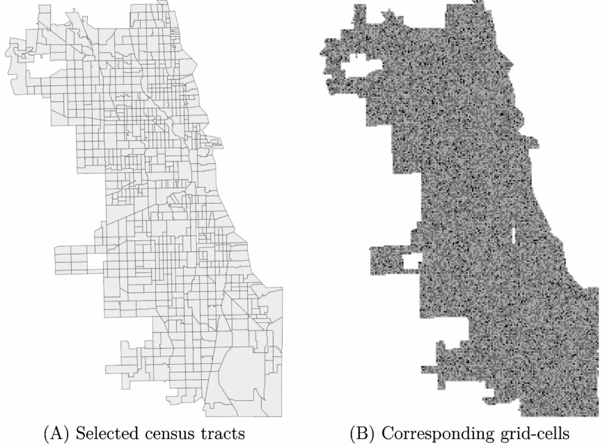
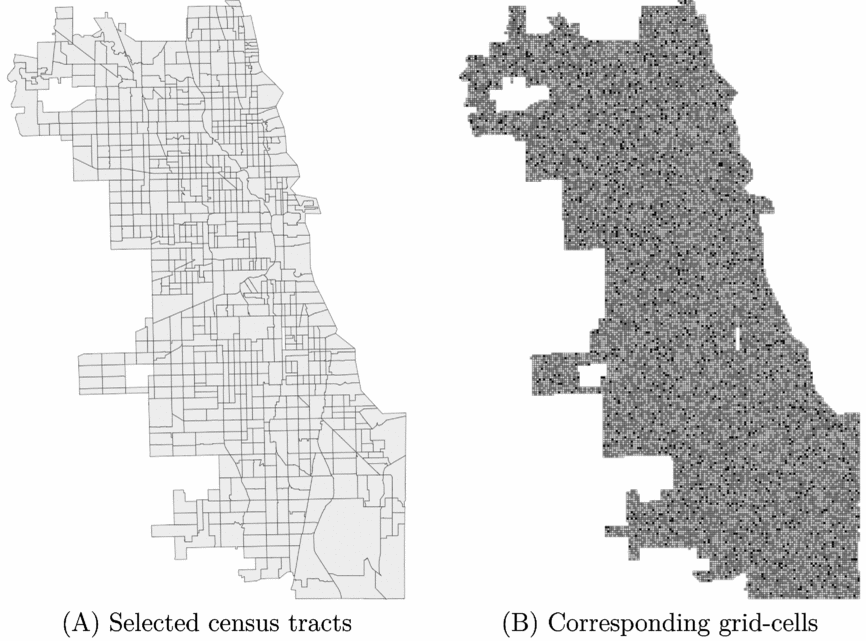
Although the spatial data shown in Figures 1 and 2 are available in vector polygon form, we converted (rasterized) the corresponding census-tract data into numbers of grid-cells in order to specify the model's context because artisoc currently does not work with polygon data.Footnote 9 The edge length of each grid-cell roughly corresponds to 150 meters, and the whole Chicago-like lattice consists of 26,507 grid-cells as shown in Figure 6. This spatial modification allows for comparing simulation outcomes with empirical observations. For simplicity, we only consider Black-White neighborhood segregation and agents in our model represent householders of each racial group.Footnote 10 As in the simulation runs above, 95% of grid-cells are populated with agents, and the same number (50%) of penny and dime agents are randomly created. We set preference threshold θ = 1/3 and ${\cal N}$ = a 7 × 7 Moore neighborhood. Model parameters π and T are also set as in the previous subsection, i.e., π = 0.95 and T = 10, 000.
Grid-cell representation of the city of Chicago Notes: Polygon-form spatial data (Panel (A)) was converted into grid-cell (raster) form (Panel (B)) using GIS data converter for artisoc. The edge length of each grid-cell roughly corresponds to 150 meters. Black cells represent empty cells. Dark gray and light gray cells represent penny and dime agents respectively. A geographically isolated tract (Federal Information Processing Standards (FIPS) code = 770602) is dropped for convenience.
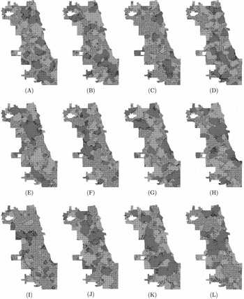
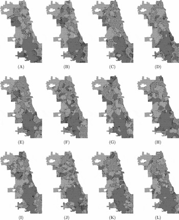
As shown in Figure 2, the Black-White segregation pattern observed in Chicago is best described as a mixture of highly segregated Black/White clusters and heterogeneous mosaics where both groups coexist, or a spatial pattern of mixed segregation and integration. Figure 7 shows twelve illustrative simulation runs. As the simulation outcomes demonstrates, our specified model yields spatial segregation patterns that contain segregated patches for each agent group as well as patches where both groups coexist within the Chicago boundary. In this sense, the specified version of the segregation model seems to be able to generate the observed pattern of segregation.
Twelve illustrative simulation runs of the specified segregation model. Notes: Each panel shows the spatial distribution of agents when it reaches to an equilibrium where all agents are satisfied with their current positions.

Indeed, we need a more comprehensive replication and statistical tests on agreements between simulation outcomes and empirical data in order to formally test and validate these preliminary results. Nonetheless, these illustrative runs visually suggest that the combination of a mild level of segregation preferences and a specific neighborhood size may be sufficient to generate the residential segregation observed in Chicago. The original Schelling's model is explainable of the level of segregation but not the form of segregation empirically observed. A slightly modified model with a greater neighborhood size is explainable of both the level and the form of segregation, but it is not obvious whether the model is applicable to the real-world cities. Our specified model demonstrates that the modified model may be applicable to the residential segregation observed in Chicago. KISS modeling enables the first two evaluations but not the last. Tightening the connection between the model and the empirical observation, TASS modeling makes such an evaluation possible.
One limitation of current model is that the spatial distribution of local clusters varies from one simulation run to another as shown in Figure 7. Because agents are randomly put at the beginning of each simulation run and the specific locations of clusters depend of the initial spatial configuration of agents, our model is not able to constantly generate a specific spatial distributions of agents similar to the observed segregation pattern. It seems that we need some deterministic and exogenous elements coupled with our model in order to constantly generate such a specific distribution of segregated clusters.
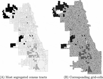
Although there are numerous possible extensions such as introduction of economic motives, geographic/physical barriers, ‘quarter’ agents representing Hispanics or Asians, and variation in the agents’ tolerance thresholds, an arbitrary ‘tuning’ of the initial spatial configuration of agents is sufficient to generate clusters in a specific part of the city.Footnote 11 Specifically, we set some ‘core communities’ of agents belonging to each group in the initial state. The agents constituting these communities behave as do other agents – the only difference is their initial spatial locations. We select roughly 10% (80/801) of census tracts dominated by either Blacks or Whites, and fill the corresponding grid-cells with penny (representing Blacks) or dime agents (representing Whites) respectively, as Figure 8 shows.Footnote 12
Distribution of the 10% most segregated census tracts and the corresponding grid-cells (‘core communities’). Notes: Panel (A) shows the spatial distribution of 80/801 most segregated census tracts dominated by either Blacks (dark gray) or Whites (black). Panel (B) shows the corresponding grid-cell representation and the spatial distribution of penny agents representing Blacks (dark gray) and dime agents representing Whites (black) at the beginning of a simulation run.

Figure 9 shows 12 illustrative simulation runs of the specified model with predetermined core communities. As shown in each panel, simulation outcomes have successfully generated segregation patterns with clusters located at specific locations. Gravitating toward the preexisting core communities, segregated clusters populated penny (dark gray) agents tend to form at the bottom and the center-left part of the lattice, and dime (light gray) clusters tend to form at the upper-left corner and the center of the lattice. This spatial distribution of segregated clusters, together with the general spatial segregation pattern of mixed segregation and integration, bear some resemblance to the observed spatial pattern.
Twelve illustrative simulation runs of the specified segregation model with ‘core communities’ Notes: Each panel shows the spatial distribution of agents when a simulation run reaches to an equilibrium where all agents are satisfied with their current positions. Note that the locations of segregated clusters become more stable than simulation runs shown in Figure 7 due to the introduction of ‘core communities’.

Indeed, such an arbitrary tuning itself tells us little about the underlying process without a reasonable interpretation of the core communities and their initial locations. Incorporating the segregation model with additional spatial data of geographycal/physical barriers, dwelling prices, or empirical evidence on segregation preferences of different racial groups might yield more theoretically and empirically relevant insights. However, providing such a comprehensive examination of the causes of residential segregation in Chicago is beyond the scope of this article. Rather, our preliminary exercise aims to demonstrate how simple, but empirically explicit agent-based models, can serve as a heuristic that help researchers examine potential inferential leverage of abstract model on specific empirical cases. Indeed, the exercise here implies that the slightly modified version of Schelling's segregation model serves as a useful heuristic to specify micro-level mechanisms sufficient, if not necessary, to generate the observed pattern of residential segregation in the city of Chicago. Extending the model such that it incorporates the model with individual-level census data or other fine-grained empirical data is likely to help researchers further clarify and test the micro-level mechanisms underlying the macro-level patterns of residential segregation as some pioneering works have already demonstrated (e.g., Benenson et al., Reference Benenson, Omer and Hatna2002, Reference Benenson, Hatna and Or2009; Bruch, Reference Bruch2014; Crooks, Reference Crooks2008; Yin, Reference Yin2009). As such, direct validation of hypothesized models is extremely difficult with conventional KISS modeling and other purely theoretical modeling techniques, the methodological utility of TASS-type ABM and the technical solution offered by GIS converter for artisoc contribute to the longstanding interests in examination of the micro-macro relationships in social sciences.
4 Conclusion and outlook
In this article, we have scrutinized the recent development of ABM and its empirical turn. While the ABM technique becomes increasingly popular in social science research, conventional models adhere to the KISS principle and are rarely tested, evaluated, or validated using empirical data, leaving the links between models and empirical phenomena rather loose. While parsimony is vital in modeling attempts and the KISS principle cannot be disregarded, temporally and spatially specified modeling, or TASS modeling provides a promising way to fill this gap. While it currently takes in-depth ABM and GIS skills to exploit opportunities offered by TASS modeling, the most recent development of softwares presents a possible solution to such technical challenges. The working example that incorporates Schelling's segregation model with geo-referenced census data has showed that TASS modeling enables us to empirically test, evaluate, and validate agent-based models using empirical data. Although successfully providing a comprehensive explanation for the residential segregation in Chicago is likely to require additional modifications and systematic replications, our preliminary exercise has demonstrated the potential methodological utility of TASS modeling.
While our working example has focused on the sociological question of urban residential segregation, the possible methodological contribution of TASS modeling is not limited to the specific research agenda. Among others, the TASS-type, empirically explicit computational approach is likely to be extremely useful in civil war study as some pioneering studies have already demonstrated (e.g., Bhavnani and Choi, Reference Bhavnani and Choi2012; Bhavnani et al., Reference Bhavnani, Miodownik and Choi2011, Reference Bhavnani, Donnay, Miodownik, Mor and Helbing2014; Lim et al., Reference Lim, Metzler and Bar-Yam2007; Weidmann and Salehyan, Reference Weidmann and Salehyan2013). The dynamics and spatial distributions of violence in civil war emerge from autonomous actions and interactions between armed groups and individuals. As hypotheses and theories of civil war mainly focus on the micro-level interactions, a methodological challenge arises: ‘The mechanisms we postulate are located at the micro-level . . . we can only observe the result of this process at the macro-level’ (Weidmann and Salehyan, Reference Weidmann and Salehyan2013: 55). TASS-type agent-based models incorporated with increasingly available detailed spatial data on violence taking place in the context of civil war, offer a methodological solution to explore the relationship between often unobserved or unobservable micro-mechanisms and observed macro-outcomes.
Indeed, TASS modeling is not a substitute but complement to existing methodologies. Nonetheless, incorporating parsimonious agent-based models with increasingly available spatial data offers a unique opportunity to systematically test and specify micro-level mechanisms underlying macro-level phenomena through computational experiments (Janssen and Ostrom, Reference Janssen and Ostrom2006; Lustick and Miodownik, Reference Lustick and Miodownik2009). As abstract KISS models can be extremely useful in developing theories, empirically grounded TASS models can help to yield empirically plausible insights. Empirically plausible TASS agent-based models could also serve as heuristic devices to assess the potential impacts of alternative policy options that would otherwise not be quantitatively comparable (e.g., Bhavnani et al., Reference Bhavnani, Donnay, Miodownik, Mor and Helbing2014; Weidmann and Salehyan, Reference Weidmann and Salehyan2013), which is likely to be of great interest to policy-makers and scholars alike.
There are also new methodological challenges for developing and testing TASS agent-based models. Among other things, effort is needed to develop commonly agreed and systematic standards for fitting models with empirical data and comparing alternative models. Currently, existing applications have used a variety of resolutions of empirical data and testing schemes, and there are no commonly applied standards. Developing such standards is likely to require accumulation of TASS modeling applications, but an effort itself may increase the acceptance of empirically grounded agent-based computational models in social sciences. We leave for future research this challenging task.
About the author
Gaku ITO is a Ph.D. student, the Department of Advanced Social and International Studies, the Graduate School of Arts and Sciences, the University of Tokyo (2012—) as well as Project Academic Support Specialist, the Department of Health Education and Sociology, the School of Public Health, the Graduate School of Medicine, the University of Tokyo (2015—). His research focuses on conflict dynamics, civil and international conflicts, and the integration of Agent-Based Modeling with Geographic Information System. He received MA in Arts and Sciences from the University of Tokyo in 2012.
Susumu YAMAKAGE is Professor of International Relations at Aoyama Gakuin University, Tokyo. Before taking the current position in 2012, he had taught International Relations at the Graduate School of Arts and Sciences, the University of Tokyo for three decades. His academic interests include the methodology of building and analyzing artificial (virtual) societies. He received Ph.D. in political science from Massachusetts Institute of Technology in 1982.