1 Introduction
The objective of this study is the nonlinear interactions between various instability modes occurring in magnetised Taylor–Couette flow, i.e. the fluid flow between independently rotating concentric cylinders. The purely hydrodynamic Taylor–Couette flow, in the absence of a magnetic field, has long served as a theoretical, numerical and experimental test bench for the study of centrifugal and shear instability mechanisms. Keeping the outer cylinder stationary, Taylor (Reference Taylor1923) observed that the flow is destabilised by purely hydrodynamic axisymmetric perturbations at a certain critical speed of the inner cylinder. The balance between rotational and shear effects can be modified by further introducing a rotation of the outer cylinder. The independent variation of the inner and outer cylinder speeds results in a rich diversity of secondary nonlinear flow patterns, as reported by Andereck, Liu & Swinney (Reference Andereck, Liu and Swinney1986). The stability and nonlinear states of Taylor–Couette flow are commonly studied in the  $R_{i}$–
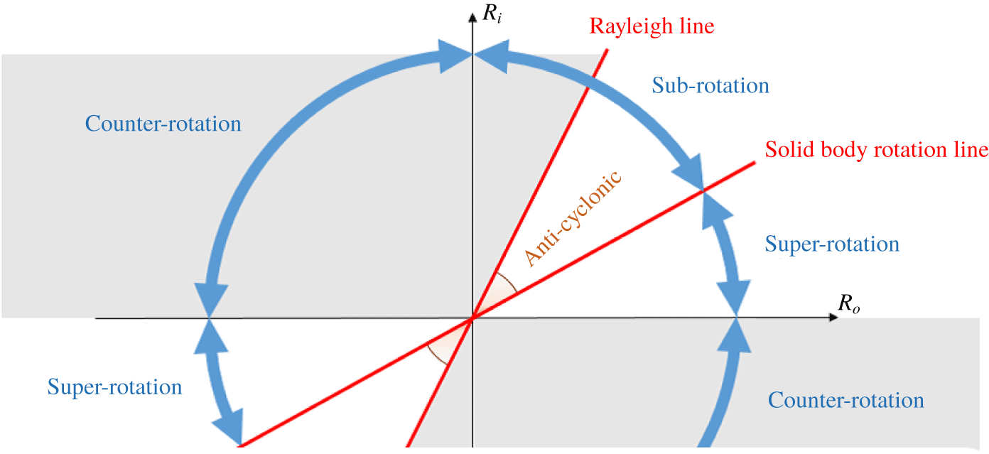
 $R_{o}$ parameter space schematically depicted in figure 1, where
 $R_{i}$ and
 $R_{o}$ are the Reynolds numbers associated with the inner and outer cylinder speeds, respectively.
In accordance with the symmetries of the problem, the  $R_{i}$–
 $R_{o}$ parameter plane is invariant to
 $\unicode[STIX]{x03C0}$ rotation about the origin, such that only the upper half-plane needs to be explored. The right/left of the half-plane corresponds to cylinders rotating in the same/opposite direction (i.e. co-rotation/counter-rotation). The first quadrant (co-rotation regime) is divided into sub-rotation and super-rotation by the solid-body rotation line (equal angular speed of the cylinders), depending on whether the outer cylinder rotates slower or faster than the inner. For any given speed of the outer cylinder, Rayleigh’s inviscid stability criterion establishes that circular Couette flow remains centrifugally stable to infinitesimal axisymmetric perturbations as long as the inner cylinder is steady or in co-rotation up to a certain speed, delimited by the so-called Rayleigh line (the wedge-shaped white region in figure 1 between the Rayleigh line and the horizontal
 $R_{i}=0$ line). Taking viscous effects and non-axisymmetric perturbations into account affects the stability boundaries, but it is widely accepted that the Rayleigh line acts as a fairly approximate threshold below which circular Couette flow remains the only stable state, given that no experimental or numerical evidence of nonlinear flow states has been found to date (see Ji et al. Reference Ji, Burin, Schartman and Goodman2006; Edlund & Ji Reference Edlund and Ji2014; Lopez & Avila Reference Lopez and Avila2017). Note, however, that no first-principles theory has been advanced so far to support the nonlinear hydrodynamic stability in the quasi-Keplerian flow regime (see Balbus (Reference Balbus2017), for a summary on the matter).
The  $R_{i}$–
 $R_{o}$ parameter space representation of Taylor–Couette flow. The plane is divided into the counter-rotation and the co-rotation regimes. This latter is further subdivided into sub-rotation and super-rotation by the solid-body rotation line defined by equal angular speeds of both cylinders. The shaded regions denote inviscid instability of circular Couette flow following the Rayleigh criterion. The portion of the sub-rotation regime between the Rayleigh and solid-body rotation lines goes by the name of anticyclonic regime (also called quasi-Keplerian), while the rest of the plane is called cyclonic.

The Rayleigh-stable region is further subdivided into the anticyclonic and super-rotation cyclonic regimes by the solid-body rotation line, corresponding to both cylinders rotating at the same angular speed. Immediately to the right of the Rayleigh line and all the way down to solid rotation, co-rotation and sub-rotation are said to be anticyclonic and laminar Couette flow is allegedly linearly stable. This region is of utmost astrophysical interest, since Keplerian rotational flow, a vastly used model for accretion disks, is precisely anticyclonic. The rate at which angular momentum is radially transported in observation of astrophysical accretion disks requires the flow to be turbulent. This has motivated a wealth of studies (see the review paper by Rüdiger et al. (Reference Rüdiger, Gellert, Hollerbach, Schultz and Stefani2018a)) exploring magneto-rotational instabilities (henceforth referred to as MRI) as a possible alternative source for turbulence in a flow that appears otherwise to always revert back to laminar in the absence of magnetic fields. The pioneering works by Velikhov (Reference Velikhov1959) and Chandrasekhar (Reference Chandrasekhar1960) showed that a uniform external magnetic field in the axial direction indeed destabilises the anticyclonic regime, while the importance of the instability in the astrophysical context was noted for the first time by Balbus & Hawley (Reference Balbus and Hawley1991). This type of MRI is nowadays called the standard type of MRI, SMRI for short.
A different approach was nevertheless taken in the first experimental observation of the MRI (Stefani et al. Reference Stefani, Gundrum, Gerbeth, Rüdiger, Schultz, Szklarski and Hollerbach2006). The SMRI is actually very difficult to reproduce in liquid-metal experiments where the magnetic Prandtl number  $P_{m}$ is very small, as magnetic induction is essential in this case. As shown by Goodman & Ji (Reference Goodman and Ji2002), the critical Reynolds number of the SMRI is inversely proportional to the magnetic Prandtl number
 $P_{m}$ for small
 $P_{m}$, meaning that the cylinders must rotate at an extremely fast rate to trigger the SMRI in the experimental apparatus. The crux in reproducing a MRI at relatively small Reynolds numbers was the numerical finding by Hollerbach & Rüdiger (Reference Hollerbach and Rüdiger2005) that, when both azimuthal and axial external magnetic fields are applied simultaneously, the critical Reynolds number saturates at a finite value even in the inductionless limit of
 $P_{m}\rightarrow 0$. Soon after the discovery of this helical MRI (henceforth referred to as HMRI), growth of axisymmetric perturbations was confirmed in the series of PROMISE experiments (Rüdiger et al. Reference Rüdiger, Hollerbach, Stefani, Gundrum, Gerbeth and Rosner2006; Stefani et al. Reference Stefani, Gundrum, Gerbeth, Rüdiger, Schultz, Szklarski and Hollerbach2006, Reference Stefani, Gundrum, Gerbeth, Rüdiger, Szklarski and Hollerbach2007). Later on, Hollerbach, Teeluck & Rüdiger (Reference Hollerbach, Teeluck and Rüdiger2010) found that non-axisymmetric modes arise instead when purely azimuthal magnetic fields are considered in the sub-rotation regime just below the Rayleigh line. They further showed that these so-called azimuthal magneto-rotational instability (AMRI) modes persist when a small axial magnetic field is added to the predominantly azimuthal field, thus implying that they could potentially interact with the axisymmetric HMRI mode. In fact, when the strengths of the azimuthal and axial external magnetic fields are suitably adjusted, the critical Reynolds numbers for the axisymmetric and non-axisymmetric modes become comparable. The competition of these modes may yield rich nonlinear flow patterns at this particular HMRI regime. This nonlinear mode interaction is the first subject we will tackle in this study.
In the early years of the pattern-formation theoretical studies in purely hydrodynamic Taylor–Couette flow, weakly nonlinear analysis was employed to investigate mode interactions among multiple linear instability modes near criticality (e.g. Davey, DiPrima & Stuart Reference Davey, DiPrima and Stuart1968; Iooss Reference Iooss1986; Golubitsky, Stewart & Schaeffer Reference Golubitsky, Stewart and Schaeffer1988; Chossat & Iooss Reference Chossat and Iooss1994). The simplest mode interaction occurs between two identical but mutually symmetric, with respect to an axial reflection, spiral modes. In this case, the fully nonlinear mixed-mode solution can be computed in numerical simulations using a periodic axial–azimuthal orthogonal domain (Tagg et al. Reference Tagg, Edwards, Swinney and Marcus1989). However, when the interacting spirals are not mutually symmetric and have a different absolute pitch, as are indeed the two mode interactions studied here, the numerical computation of the fully nonlinear mixed mode is no longer straightforward. The periodic computational domain must fit an integer number of both constituent modes in order to faithfully reproduce the mixed mode, which may lead to unaffordably large domains. This may be feasible on some occasions (Avila, Meseguer & Marques Reference Avila, Meseguer and Marques2006; Pinter, Lücke & Hoffmann Reference Pinter, Lücke and Hoffmann2006; Altmeyer & Hoffmann Reference Altmeyer and Hoffmann2010), but it is at the very least inefficient from a computational point of view, if not altogether prohibitive. A convenient methodology for the computation of general mixed-mode states was provided by Deguchi & Altmeyer (Reference Deguchi and Altmeyer2013), who realised that the infinite annulus might be subdivided into a regular tiling of a suitable parallelogram-shaped periodic box that can be chosen optimally small for any flow pattern arising from nonlinear interaction of two modes, as we are considering here. Extension of the nonlinear code to magnetised problems might prove highly valuable to the study of MRI, as nonlinear simulations in cylindrical/annular domains have only recently been undertaken (Guseva et al. Reference Guseva, Willis, Hollerbach and Avila2015, Reference Guseva, Willis, Hollerbach and Avila2017).
In the second half of this paper we shall also study the nonlinear mode competition occurring in the other Rayleigh-stable regime, i.e. the super-rotation regime seen in figure 1. Recently, magnetohydrodynamic (MHD) instabilities in this regime have attracted much attention as they are thought to be relevant for turbulence generation in a part of the Sun’s tachocline. In this second subject we shall investigate the nonlinear competition of two recently discovered linear instability modes.
For the purely hydrodynamic problem, non-laminar flow patterns in the inviscidly stable super-rotation regime were first reported several decades ago in Taylor–Couette experiments by Wendt (Reference Wendt1933) and Coles (Reference Coles1965), but at the time it was not clear whether the instability was legitimate or an endwall effect induced by the cylinder lids. Advances in computational power eventually allowed numerical confirmation of the existence of subcritical spiral turbulence and intermittency found experimentally (Van Atta Reference Van Atta1966; Hegseth et al. Reference Hegseth, Andereck, Hayot and Pomeau1989; Prigent et al. Reference Prigent, Gregoire, Chate, Dauchot and van Saarloos2002; Burin & Czarnocki Reference Burin and Czarnocki2012) in the counter-rotation regime in the absence of endwall effects (Dong Reference Dong2009; Meseguer et al. Reference Meseguer, Mellibovsky, Avila and Marques2009). Nonlinear coherent states have indeed been followed into the super-rotation regime, crossing the  $R_{i}=0$ boundary, as illustrated by the computation of the first rotating wave in cyclonic super-rotation (Deguchi, Meseguer & Mellibovsky Reference Deguchi, Meseguer and Mellibovsky2014) and by direct numerical simulation (Ostilla-Monico, Verzicco & Lohse Reference Ostilla-Monico, Verzicco and Lohse2016). All non-trivial flow patterns hitherto observed in super-rotation are finite-amplitude and highly nonlinear, such that they by no means belie the widely assumed linear stability of super-rotating hydrodynamic Taylor–Couette flow, in view of countless numerical studies of the neutral curve (see the review article by Grossmann, Lohse & Sun (Reference Grossmann, Lohse and Sun2016)). The recent unexpected discovery by Deguchi (Reference Deguchi2017) of a linear instability in the super-rotation regime therefore came as a big surprise. Considering non-axisymmetric perturbations and a relatively long axial wavelength were key ingredients to the finding. This instability mode of a purely hydrodynamic nature, hereafter called the D17 mode, is the first of the two modes we shall consider in our second mode competition study.
The other mode at play inherently originates from the MRI mechanism and is called the super-AMRI (Rüdiger et al. Reference Rüdiger, Schultz, Gellert and Stefani2016, Reference Rüdiger, Schultz, Gellert and Stefani2018b), where the prefix ‘super’ refers to the super-rotation regime. This mode belongs, along with the usual forms of HMRI and AMRI for sub-rotation, to the class of inductionless MRI. It has long been known that MRI is not easily triggered in the super-rotation regime for the axisymmetric case. For ideal fluids, Velikhov’s condition states that the axial magnetic field cannot destabilise this regime (Velikhov Reference Velikhov1959), while according to Michael’s condition (Michael Reference Michael1954), an azimuthal field can only be destabilising provided its modulus increases outwards at a sufficiently fast rate. Moreover, when the azimuthal magnetic field is current-free, it can be formally shown that axisymmetric MRI are impossible in spite of the diffusive effect (Herron & Soliman Reference Herron and Soliman2006). A breakthrough regarding instability in the cyclonic super-rotation regime is due to Stefani & Kirillov (Reference Stefani and Kirillov2015), who pointed out that for sufficiently narrow gaps the non-axisymmetric instability could be continued into the super-rotation regime using the so-called local approximation and the inductionless limit ( $P_{m}\rightarrow 0$). However, the existence of the super-AMRI was not conclusive at this stage given that a local approximation does not always necessarily provide accurate insight into the global problem. Soon after, conclusive numerical evidence of the super-AMRI was reported by Rüdiger et al. (Reference Rüdiger, Schultz, Gellert and Stefani2016, Reference Rüdiger, Schultz, Gellert and Stefani2018b), who concluded that the destabilisation seems to occur for fairly arbitrary magnetic field profiles as long as the flow is double-diffusive, i.e.
 $P_{m}\neq 1$.
The paper is organised as follows. Section 2 formulates the problem based on the inductionless limit of the MHD equations. The section addresses in detail the numerical discretisation of the equations in annular-parallelogram periodic domains and, in particular, describes the Newton solver for the computation of nonlinear mixed-mode travelling waves using the transformed coordinate system and a suitable co-moving reference frame. Section 3 is devoted to the anticyclonic regime. The helical magnetic field is imposed to find the nonlinear mixed-mode solutions that arise from the mode competition advanced by Hollerbach et al. (Reference Hollerbach, Teeluck and Rüdiger2010). The first part of § 4 deals with the interaction between the classical non-axisymmetric and the D17 modes in purely hydrodynamic counter-rotating Taylor–Couette flow. In the second half of § 4 we shall see how an imposed azimuthal magnetic field alters the nature of this interaction. Finally, in § 5, we briefly summarise the results and present concluding remarks.
2 Formulation of the problem
Consider an electrically conducting fluid of density  $\unicode[STIX]{x1D70C}^{\ast }$, kinematic viscosity
 $\unicode[STIX]{x1D708}^{\ast }$ and magnetic diffusivity
 $\unicode[STIX]{x1D702}^{\ast }$, confined between two concentric cylinders of inner and outer radii
 $r_{i}^{\ast }$ and
 $r_{o}^{\ast }$, independently rotating at angular speeds
 $\unicode[STIX]{x1D6FA}_{i}^{\ast }$ and
 $\unicode[STIX]{x1D6FA}_{o}^{\ast }$, respectively. In addition, the fluid is subject to the action of a magnetic field of typical strength
 $B_{0}^{\ast }$. Throughout the paper we use the length
 $d^{\ast }=r_{o}^{\ast }-r_{i}^{\ast }$, time
 $d^{\ast 2}/\unicode[STIX]{x1D708}^{\ast }$, velocity
 $\unicode[STIX]{x1D708}^{\ast }/d^{\ast }$ and magnetic field
 $\unicode[STIX]{x1D708}^{\ast }\sqrt{\unicode[STIX]{x1D70C}^{\ast }\unicode[STIX]{x1D707}^{\ast }}/d^{\ast }$ scales for non-dimensionalisation, where
 $\unicode[STIX]{x1D707}^{\ast }$ is the magnetic permeability. As a consequence of using the viscous time scale, the Reynolds numbers are absorbed into the expression for the base-state flow fields and disappear from the non-dimensional equations for the perturbation. The key parameters of the flow are the radius ratio
 $\unicode[STIX]{x1D702}$, the inner
 $R_{i}$ and outer
 $R_{o}$ Reynolds numbers, along with the magnetic Prandtl number
 $P_{m}$ and the Hartmann number
 $H$:
 $$\begin{eqnarray}\unicode[STIX]{x1D702}=\frac{r_{i}^{\ast }}{r_{o}^{\ast }},\quad R_{i}=\frac{\unicode[STIX]{x1D6FA}_{i}^{\ast }r_{i}^{\ast }d^{\ast }}{\unicode[STIX]{x1D708}^{\ast }},\quad R_{o}=\frac{\unicode[STIX]{x1D6FA}_{o}^{\ast }r_{o}^{\ast }d^{\ast }}{\unicode[STIX]{x1D708}^{\ast }},\quad P_{m}=\frac{\unicode[STIX]{x1D708}^{\ast }}{\unicode[STIX]{x1D702}^{\ast }},\quad H=\frac{B_{0}^{\ast }d^{\ast }}{\sqrt{\unicode[STIX]{x1D70C}^{\ast }\unicode[STIX]{x1D707}^{\ast }\unicode[STIX]{x1D702}^{\ast }\unicode[STIX]{x1D708}^{\ast }}}.\end{eqnarray}$$
The non-dimensional external magnetic field is proportional to  $P_{m}^{-1/2}H$. The reason for using
 $H$ is that we will consider the so-called inductionless limit
 $P_{m}\rightarrow 0$ where
 $H$ is typically fixed as a constant.
Non-dimensionalisation of the velocity field  $\boldsymbol{v}=u\boldsymbol{e}_{r}+v\boldsymbol{e}_{\unicode[STIX]{x1D703}}+w\boldsymbol{e}_{z}$ and magnetic field
 $\boldsymbol{B}=A\boldsymbol{e}_{r}+B\boldsymbol{e}_{\unicode[STIX]{x1D703}}+C\boldsymbol{e}_{z}$, expressed here in cylindrical coordinates
 $(r,\unicode[STIX]{x1D703},z)$, yields the incompressible viscous–resistive MHD equations:
 $$\begin{eqnarray}\displaystyle & \displaystyle \unicode[STIX]{x2202}_{t}\boldsymbol{v}+(\boldsymbol{v}\boldsymbol{\cdot }\unicode[STIX]{x1D735})\boldsymbol{v}-(\boldsymbol{B}\boldsymbol{\cdot }\unicode[STIX]{x1D735})\boldsymbol{B}=-\unicode[STIX]{x1D735}p+\unicode[STIX]{x1D6FB}^{2}\boldsymbol{v}, & \displaystyle\end{eqnarray}$$
 $$\begin{eqnarray}\displaystyle & \displaystyle \unicode[STIX]{x2202}_{t}\boldsymbol{B}+(\boldsymbol{v}\boldsymbol{\cdot }\unicode[STIX]{x1D735})\boldsymbol{B}-(\boldsymbol{B}\boldsymbol{\cdot }\unicode[STIX]{x1D735})\boldsymbol{v}=P_{m}^{-1}\unicode[STIX]{x1D6FB}^{2}\boldsymbol{B}, & \displaystyle\end{eqnarray}$$
 $$\begin{eqnarray}\displaystyle & \displaystyle \unicode[STIX]{x1D735}\boldsymbol{\cdot }\boldsymbol{v}=\unicode[STIX]{x1D735}\boldsymbol{\cdot }\boldsymbol{B}=0, & \displaystyle\end{eqnarray}$$
 $p$ is the total pressure and
 $t$ is time. Equation (2.2a) expresses momentum conservation, while equation (2.2b) is the induction equation. Equation (2.2c) corresponds to continuity and Gauss’ law. Along the cylinder walls at radii
 $$\begin{eqnarray}r_{i}=\frac{\unicode[STIX]{x1D702}}{1-\unicode[STIX]{x1D702}},\quad r_{o}=\frac{1}{1-\unicode[STIX]{x1D702}},\end{eqnarray}$$
we assume no-slip and perfectly insulating boundary conditions. In our formulation, the velocity and magnetic fields are decomposed into the base and the perturbation flows following
 $$\begin{eqnarray}\displaystyle & \displaystyle \boldsymbol{v}=v_{b}(r)\boldsymbol{e}_{\unicode[STIX]{x1D703}}+Gw_{p}(r)\boldsymbol{e}_{z}+\widetilde{\boldsymbol{v}}(r,\unicode[STIX]{x1D703},z,t), & \displaystyle\end{eqnarray}$$
 $$\begin{eqnarray}\displaystyle & \displaystyle \boldsymbol{B}=P_{m}^{-1/2}H\{B_{b}(r)\boldsymbol{e}_{\unicode[STIX]{x1D703}}+C_{b}(r)\boldsymbol{e}_{z}\}+\widetilde{\boldsymbol{B}}(r,\unicode[STIX]{x1D703},z,t), & \displaystyle\end{eqnarray}$$
 $\widetilde{p}$. Here
 $v_{b}(r)=R_{s}r+R_{p}r^{-1}$ is the laminar Couette flow solution, with coefficients
 $$\begin{eqnarray}R_{s}=\frac{R_{o}-\unicode[STIX]{x1D702}R_{i}}{1+\unicode[STIX]{x1D702}},\quad R_{p}=\frac{\unicode[STIX]{x1D702}^{-1}R_{i}-R_{o}}{1+\unicode[STIX]{x1D702}}r_{i}^{2},\end{eqnarray}$$
where the subscripts denote the solid-body rotation ( $s$) and the potential (
 $p$) components of the flow. External magnetic mechanisms induce the base magnetic fields
 $B_{b}(r)$ and
 $C_{b}(r)$, which will be duly introduced in (3.1) and (4.1) for the two types of predominantly azimuthal fields that will be considered throughout the paper.
We will assume further that there is no axial net mass flux. This is accomplished by imposing an external instantaneously adjustable axial pressure gradient that induces the well-known base annular Poiseuille flow profile:
 $$\begin{eqnarray}w_{p}(r)=(r^{2}-r_{i}^{2})\ln r_{o}+(r_{o}^{2}-r^{2})\ln r_{i}-(r_{o}^{2}-r_{i}^{2})\ln r.\end{eqnarray}$$
The product  $Gw_{p}$ in (2.4a) represents the axial flow induced by the external pressure gradient, whose strength is measured by the coefficient
 $G$. That coefficient is a time-dependent additional unknown in the constant-mass flux problem. For travelling wave states
 $G$ is merely a constant. Moreover, it is easy to show that, when the flow possesses some symmetry in
 $z$,
 $G$ must vanish.
For liquid metals used in laboratory experiments  $P_{m}$ is very small
 $(10^{-5}{-}10^{-7})$. It is therefore reasonable to apply the inductionless limit approximation
 $P_{m}\rightarrow 0$ to the governing equations (see e.g. Davidson Reference Davidson2017). The magnetic field perturbation is rescaled as
 $\widetilde{\boldsymbol{b}}=P_{m}^{-1/2}H^{-1}\widetilde{\boldsymbol{B}}$ and the size of the variables
 $\widetilde{\boldsymbol{v}},~\widetilde{\boldsymbol{b}},~\widetilde{p}$ and
 $R_{i},~R_{o},~H$ are fixed as
 $O(P_{m}^{0})$ quantities during the limiting process. The resulting leading-order equations are
 $$\begin{eqnarray}\displaystyle & & \displaystyle \left[\begin{array}{@{}c@{}}(\unicode[STIX]{x2202}_{t}+r^{-1}v_{b}\unicode[STIX]{x2202}_{\unicode[STIX]{x1D703}}+R_{p}w_{p}\unicode[STIX]{x2202}_{z})\widetilde{u}-2r^{-1}v_{b}\widetilde{v}\\ (\unicode[STIX]{x2202}_{t}+r^{-1}v_{b}\unicode[STIX]{x2202}_{\unicode[STIX]{x1D703}}+R_{p}w_{p}\unicode[STIX]{x2202}_{z})\widetilde{v}+r^{-1}(rv_{b})^{\prime }\widetilde{u}\\ (\unicode[STIX]{x2202}_{t}+r^{-1}v_{b}\unicode[STIX]{x2202}_{\unicode[STIX]{x1D703}}+R_{p}w_{p}\unicode[STIX]{x2202}_{z})\widetilde{w}\end{array}\right]\nonumber\\ \displaystyle & & \displaystyle \quad -\,H^{2}\left[\begin{array}{@{}c@{}}(r^{-1}B_{b}\unicode[STIX]{x2202}_{\unicode[STIX]{x1D703}}+C_{b}\unicode[STIX]{x2202}_{z})\widetilde{a}-2r^{-1}B_{b}\widetilde{b}\\ (r^{-1}B_{b}\unicode[STIX]{x2202}_{\unicode[STIX]{x1D703}}+C_{b}\unicode[STIX]{x2202}_{z})\widetilde{b}+r^{-1}(rB_{b})^{\prime }\widetilde{a}\\ (r^{-1}B_{b}\unicode[STIX]{x2202}_{\unicode[STIX]{x1D703}}+C_{b}\unicode[STIX]{x2202}_{z})\widetilde{c}\end{array}\right]+(\widetilde{\boldsymbol{v}}\boldsymbol{\cdot }\unicode[STIX]{x1D735})\widetilde{\boldsymbol{v}}=-\unicode[STIX]{x1D735}\widetilde{p}+\unicode[STIX]{x1D6FB}^{2}\widetilde{\boldsymbol{v}},\end{eqnarray}$$
and
 $$\begin{eqnarray}-\left[\begin{array}{@{}c@{}}(r^{-1}B_{b}\unicode[STIX]{x2202}_{\unicode[STIX]{x1D703}}+C_{b}\unicode[STIX]{x2202}_{z})\widetilde{u}\\ (r^{-1}B_{b}\unicode[STIX]{x2202}_{\unicode[STIX]{x1D703}}+C_{b}\unicode[STIX]{x2202}_{z})\widetilde{v}-r(r^{-1}B_{b})^{\prime }\widetilde{u}\\ (r^{-1}B_{b}\unicode[STIX]{x2202}_{\unicode[STIX]{x1D703}}+C_{b}\unicode[STIX]{x2202}_{z})\widetilde{w}\end{array}\right]=\unicode[STIX]{x1D6FB}^{2}\widetilde{\boldsymbol{b}},\end{eqnarray}$$
along with the solenoidal conditions  $\unicode[STIX]{x1D735}\boldsymbol{\cdot }\widetilde{\boldsymbol{v}}=\unicode[STIX]{x1D735}\boldsymbol{\cdot }\widetilde{\boldsymbol{b}}=0$. The time derivative drops out from the induction equations on account of applying the inductionless limit, and (2.7b) becomes a mere linear system linking the velocity and the magnetic field. It can thus be used, as will be shown shortly, to eliminate the magnetic perturbation from the momentum equation (2.7a).
2.1 Spectral discretisation on a parallelogram domain
We shall be looking here for nonlinear travelling wave solutions of the above resulting equations. The hydrodynamic and magnetic perturbation fields  $\widetilde{\boldsymbol{v}}$ and
 $\widetilde{\boldsymbol{b}}$ are both solenoidal, so they admit a toroidal–poloidal decomposition of the form
 $$\begin{eqnarray}\displaystyle & \displaystyle \widetilde{\boldsymbol{v}}(r,\unicode[STIX]{x1D703},z,t)=\boldsymbol{e}_{\unicode[STIX]{x1D703}}\overline{v}(r)+\boldsymbol{e}_{z}\overline{w}(r)+\unicode[STIX]{x1D735}\times \unicode[STIX]{x1D735}\times \{\boldsymbol{e}_{r}\unicode[STIX]{x1D719}(r,\unicode[STIX]{x1D703},z,t)\}+\unicode[STIX]{x1D735}\times \{\boldsymbol{e}_{r}\unicode[STIX]{x1D713}(r,\unicode[STIX]{x1D703},z,t)\}, & \displaystyle \nonumber\\ \displaystyle & & \displaystyle\end{eqnarray}$$
 $$\begin{eqnarray}\displaystyle & \displaystyle \widetilde{\boldsymbol{b}}(r,\unicode[STIX]{x1D703},z,t)=\unicode[STIX]{x1D735}\times \unicode[STIX]{x1D735}\times \{\boldsymbol{e}_{r}f(r,\unicode[STIX]{x1D703},z,t)\}+\unicode[STIX]{x1D735}\times \{\boldsymbol{e}_{r}g(r,\unicode[STIX]{x1D703},z,t)\}, & \displaystyle\end{eqnarray}$$
 $\overline{v}(r)$ and
 $\overline{w}(r)$ are the azimuthal and axial components, respectively, of the mean velocity field. It can be easily shown that no mean magnetic field can be generated in the inductionless limit. The poloidal and toroidal potentials
 $\unicode[STIX]{x1D719},~f$ and
 $\unicode[STIX]{x1D713},~g$ introduced in (2.8a) and (2.8b) uniquely determine the physical hydrodynamic and magnetic perturbation fields
 $\widetilde{\boldsymbol{v}}$ and
 $\widetilde{\boldsymbol{b}}$, except for the obvious gauge freedom (addition of a constant).
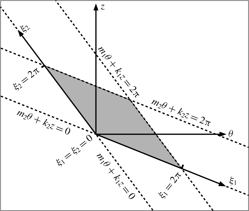
The coherent flows addressed in this work are mixed modes resulting from the nonlinear interaction of pairs of spiral waves propagating in the  $\unicode[STIX]{x1D703}{-}z$ plane. Following Deguchi & Altmeyer (Reference Deguchi and Altmeyer2013), we introduce the two phase variables
 $$\begin{eqnarray}\unicode[STIX]{x1D709}_{1}=m_{1}\unicode[STIX]{x1D703}+k_{1}z-c_{1}t,\quad \unicode[STIX]{x1D709}_{2}=m_{2}\unicode[STIX]{x1D703}+k_{2}z-c_{2}t,\end{eqnarray}$$
describing the wavefronts of the two interacting spirals, which propagate at speeds  $c_{1}$ and
 $c_{2}$, and whose azimuthal and axial wavenumbers are the integer
 $(m_{1},m_{2})$ and real
 $(k_{1},k_{2})$ constant pairs, respectively. Travelling mixed modes resulting from the nonlinear interaction of spiral modes of the form given by (2.9) are naturally represented on doubly
 $2\unicode[STIX]{x03C0}$-periodic parallelogram domains of the form
 $$\begin{eqnarray}(r,\unicode[STIX]{x1D709}_{1},\unicode[STIX]{x1D709}_{2})\in [r_{i},r_{o}]\times [0,2\unicode[STIX]{x03C0}]\times [0,2\unicode[STIX]{x03C0}],\end{eqnarray}$$
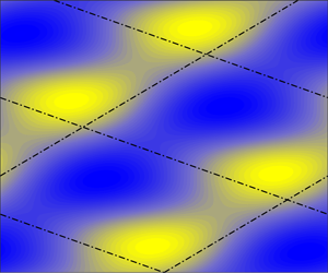
unwrapped and outlined in figure 2 for any given value of the radial coordinate. Straightforward algebraic manipulation shows that any function of  $\unicode[STIX]{x1D709}_{1}$ and
 $\unicode[STIX]{x1D709}_{2}$ can also be written in terms of
 $\unicode[STIX]{x1D703}-c_{\unicode[STIX]{x1D703}}t$ and
 $z-c_{z}t$ with
 $$\begin{eqnarray}c_{\unicode[STIX]{x1D703}}=\frac{k_{2}c_{1}-k_{1}c_{2}}{m_{2}k_{1}-m_{1}k_{2}},\quad c_{z}=\frac{m_{2}c_{1}-m_{1}c_{2}}{m_{2}k_{1}-m_{1}k_{2}}.\end{eqnarray}$$
The solutions sought are therefore travelling waves propagating both azimuthally and axially with the phase speeds  $c_{\unicode[STIX]{x1D703}}$ and
 $c_{z}$ just given, respectively.
Sketch of the parallelogram domain introducing the new variables  $(\unicode[STIX]{x1D709}_{1},\unicode[STIX]{x1D709}_{2})$ that replace the usual azimuthal and axial coordinates
 $(\unicode[STIX]{x1D703},z)$.

The initial–boundary value problem (2.7a)–(2.7b) is reformulated in the new phase variables assuming  $2\unicode[STIX]{x03C0}$-periodicity of the toroidal and poloidal potentials introduced in (2.8a)–(2.8b):
 $$\begin{eqnarray}[\unicode[STIX]{x1D719},\unicode[STIX]{x1D713},f,g](r,\unicode[STIX]{x1D709}_{1}+2\unicode[STIX]{x03C0},\unicode[STIX]{x1D709}_{2})=[\unicode[STIX]{x1D719},\unicode[STIX]{x1D713},f,g](r,\unicode[STIX]{x1D709}_{1},\unicode[STIX]{x1D709}_{2}+2\unicode[STIX]{x03C0})=[\unicode[STIX]{x1D719},\unicode[STIX]{x1D713},f,g](r,\unicode[STIX]{x1D709}_{1},\unicode[STIX]{x1D709}_{2}).\end{eqnarray}$$
The potentials are then discretised using spectral Fourier expansions of the form
 $$\begin{eqnarray}\displaystyle & \displaystyle \unicode[STIX]{x1D719}(r,\unicode[STIX]{x1D709}_{1},\unicode[STIX]{x1D709}_{2})=\mathop{\sum }_{n_{1},n_{2}}\widehat{\unicode[STIX]{x1D719}}_{n_{1}n_{2}}(r)\text{e}^{\text{i}(n_{1}\unicode[STIX]{x1D709}_{1}+n_{2}\unicode[STIX]{x1D709}_{2})},\quad \unicode[STIX]{x1D713}(r,\unicode[STIX]{x1D709}_{1},\unicode[STIX]{x1D709}_{2})=\mathop{\sum }_{n_{1},n_{2}}\widehat{\unicode[STIX]{x1D713}}_{n_{1}n_{2}}(r)\text{e}^{\text{i}(n_{1}\unicode[STIX]{x1D709}_{1}+n_{2}\unicode[STIX]{x1D709}_{2})},\qquad & \displaystyle\end{eqnarray}$$
 $$\begin{eqnarray}\displaystyle & \displaystyle f(r,\unicode[STIX]{x1D709}_{1},\unicode[STIX]{x1D709}_{2})=\mathop{\sum }_{n_{1},n_{2}}\,\widehat{f}_{n_{1}n_{2}}(r)\text{e}^{\text{i}(n_{1}\unicode[STIX]{x1D709}_{1}+n_{2}\unicode[STIX]{x1D709}_{2})},\quad g(r,\unicode[STIX]{x1D709}_{1},\unicode[STIX]{x1D709}_{2})=\mathop{\sum }_{n_{1},n_{2}}\widehat{g}_{n_{1}n_{2}}(r)\text{e}^{\text{i}(n_{1}\unicode[STIX]{x1D709}_{1}+n_{2}\unicode[STIX]{x1D709}_{2})},\qquad & \displaystyle\end{eqnarray}$$
 $\widehat{\unicode[STIX]{x1D719}}_{n_{1}n_{2}}(r)$,
 $\widehat{\unicode[STIX]{x1D713}}_{n_{1}n_{2}}(r)$,
 $\widehat{f}_{n_{1}n_{2}}(r)$ and
 $\widehat{g}_{n_{1}n_{2}}(r)$ are identically zero for
 $n_{1}=n_{2}=0$. For
 $n_{1}\neq 0$ or
 $n_{2}\neq 0$, these radial functions are suitable expansions of modified Chebyshev polynomials satisfying homogeneous no-slip boundary conditions at the inner and outer cylinder walls:
 $$\begin{eqnarray}\unicode[STIX]{x1D719}=\unicode[STIX]{x2202}_{r}\unicode[STIX]{x1D719}=\unicode[STIX]{x1D713}=\overline{v}=\overline{w}=0.\end{eqnarray}$$
The hydrodynamic radial functions are thus
 $$\begin{eqnarray}\displaystyle & \displaystyle \widehat{\unicode[STIX]{x1D719}}_{n_{1}n_{2}}(r)=\mathop{\sum }_{l}X_{ln_{1}n_{2}}^{(1)}(1-y^{2})^{2}T_{l}(y),\quad \widehat{\unicode[STIX]{x1D713}}_{n_{1}n_{2}}(r)=\mathop{\sum }_{l}X_{ln_{1}n_{2}}^{(2)}(1-y^{2})T_{l}(y), & \displaystyle\end{eqnarray}$$
 $$\begin{eqnarray}\displaystyle & \displaystyle \overline{v}(r)=\mathop{\sum }_{l}X_{l00}^{(1)}(1-y^{2})T_{l}(y),\quad \overline{w}(r)=\mathop{\sum }_{l}X_{l00}^{(2)}(1-y^{2})T_{l}(y), & \displaystyle\end{eqnarray}$$
 $T_{l}(y)$ is the
 $l$th Chebyshev polynomial and
 $y\equiv 2(r-r_{i})-1\in [-1,1]$ is the rescaled radial coordinate. Similarly, the magnetic radial functions are expanded employing Chebyshev polynomials modified to satisfy perfectly insulating conditions:
 $$\begin{eqnarray}\displaystyle & \displaystyle \widehat{f}_{n_{1}n_{2}}(r)=\mathop{\sum }_{l}X_{ln_{1}n_{2}}^{(3)}\{(1-y^{2})T_{l}(y)+\unicode[STIX]{x1D6FC}_{ln_{1}n_{2}}+\unicode[STIX]{x1D6FD}_{ln_{1}n_{2}}y\}, & \displaystyle\end{eqnarray}$$
 $$\begin{eqnarray}\displaystyle & \displaystyle \widehat{g}_{n_{1}n_{2}}(r)=\unicode[STIX]{x1D6FE}_{n_{1}n_{2}}(r)\,\widehat{f}_{n_{1}n_{2}}(r)+\mathop{\sum }_{l}X_{ln_{1}n_{2}}^{(4)}(1-y^{2})T_{l}(y). & \displaystyle\end{eqnarray}$$
 $\unicode[STIX]{x1D6FC}_{ln_{1}n_{2}}$ and
 $\unicode[STIX]{x1D6FD}_{ln_{1}n_{2}}$ and of the function
 $\unicode[STIX]{x1D6FE}_{n_{1}n_{2}}(r)$ can be found in appendix A.
For computational purposes, the Fourier–Chebyshev expansions (2.15a)–(2.16b) are truncated at  $l=L$,
 $|n_{1}|=N_{1}$ and
 $|n_{2}|=N_{2}$. After substituting the truncated expansions into system (2.7a)–(2.7b), these are then evaluated at the Chebyshev nodes
 $$\begin{eqnarray}y=\cos \left(\frac{l+1}{L+2}\unicode[STIX]{x03C0}\right),\quad l=1,\ldots ,L.\end{eqnarray}$$
This procedure leads to a system of nonlinear algebraic equations of the form
 $$\begin{eqnarray}\displaystyle & \displaystyle 0=\unicode[STIX]{x1D647}_{1}\left[\begin{array}{@{}c@{}}X_{ln_{1}n_{2}}^{(1)}\\ X_{ln_{1}n_{2}}^{(2)}\end{array}\right]+H^{2}\unicode[STIX]{x1D647}_{2}\left[\begin{array}{@{}c@{}}X_{ln_{1}n_{2}}^{(3)}\\ X_{ln_{1}n_{2}}^{(4)}\end{array}\right]+[X_{ln_{1}n_{2}}^{(1)},X_{ln_{1}n_{2}}^{(2)}]\unicode[STIX]{x1D649}\left[\begin{array}{@{}c@{}}X_{ln_{1}n_{2}}^{(1)}\\ X_{ln_{1}n_{2}}^{(2)}\end{array}\right], & \displaystyle\end{eqnarray}$$
 $$\begin{eqnarray}\displaystyle & \displaystyle \unicode[STIX]{x1D647}_{3}\left[\begin{array}{@{}c@{}}X_{ln_{1}n_{2}}^{(1)}\\ X_{ln_{1}n_{2}}^{(2)}\end{array}\right]=\unicode[STIX]{x1D647}_{4}\left[\begin{array}{@{}c@{}}X_{ln_{1}n_{2}}^{(3)}\\ X_{ln_{1}n_{2}}^{(4)}\end{array}\right]. & \displaystyle\end{eqnarray}$$
 $\unicode[STIX]{x1D647}_{1},~\unicode[STIX]{x1D647}_{2},~\unicode[STIX]{x1D647}_{3}$ and
 $\unicode[STIX]{x1D647}_{4}$ are matrices, and
 $\unicode[STIX]{x1D649}$ is a third-order tensor, whose form is unchanged from the purely hydrodynamic case. Isolating the magnetic unknowns by solving the linear system (2.18b) and substituting into (2.18a) yields a nonlinear system of equations for the hydrodynamic unknowns
 $X_{ln_{1}n_{2}}^{(1)}$ and
 $X_{ln_{1}n_{2}}^{(2)}$:
 $$\begin{eqnarray}0=(\unicode[STIX]{x1D647}_{1}+H^{2}\unicode[STIX]{x1D647}_{2}\unicode[STIX]{x1D647}_{4}^{-1}\unicode[STIX]{x1D647}_{3})\left[\begin{array}{@{}c@{}}X_{ln_{1}n_{2}}^{(1)}\\ X_{ln_{1}n_{2}}^{(2)}\end{array}\right]+[X_{ln_{1}n_{2}}^{(1)},X_{ln_{1}n_{2}}^{(2)}]\unicode[STIX]{x1D649}\left[\begin{array}{@{}c@{}}X_{ln_{1}n_{2}}^{(1)}\\ X_{ln_{1}n_{2}}^{(2)}\end{array}\right].\end{eqnarray}$$
Matrix  $\unicode[STIX]{x1D647}_{1}$ depends implicitly on the unknown speeds
 $c_{1}$ and
 $c_{2}$ appearing in (2.9), which correspond to the co-moving reference frame in which the mixed mode remains a steady solution. Since these two speeds are also unknown, two additional phase-locking conditions are required to lift the rotational/travelling degeneracy of solutions from the system of equations. Similarly, system (2.19) must also be complemented with an additional constraint to allow determination of the unknown axial pressure gradient
 $G$ required to ensure the zero-mass-flux condition. The nonlinear system (2.19), along with the aforementioned constraints, is solved numerically using Newton’s method. The hydrodynamic part of the code is identical to that used in Deguchi & Altmeyer (Reference Deguchi and Altmeyer2013), and more detailed documentation of the computational methodology can be found in Deguchi & Nagata (Reference Deguchi and Nagata2011).
For the purely hydrodynamic problem, we have also computed and continued in parameter space the bifurcating mixed modes using an independent numerical formulation. This alternative methodology is based on a solenoidal Petrov–Galerkin scheme described in Meseguer et al. (Reference Meseguer, Avila, Mellibovsky and Marques2007), suitably adapted to the annular parallelogram domain (2.10). In this formulation, the solenoidal velocity perturbation  $\widetilde{\boldsymbol{v}}$ is approximated by means of a spectral expansion
 $\widetilde{\boldsymbol{v}}_{s}$ of order
 $N$ in
 $\unicode[STIX]{x1D709}_{1}=m_{1}\unicode[STIX]{x1D703}+k_{1}z$, order
 $L$ in
 $\unicode[STIX]{x1D709}_{2}=m_{2}\unicode[STIX]{x1D703}+k_{2}z$, and order
 $M$ in
 $r$:
 $$\begin{eqnarray}\widetilde{\boldsymbol{v}}_{s}(r,\unicode[STIX]{x1D709}_{1},\unicode[STIX]{x1D709}_{2},t)=\mathop{\sum }_{n_{1},\,n_{2},\,m}a_{n_{1}n_{2}m}(t)\,\unicode[STIX]{x1D731}_{n_{1}n_{2}m}(r,\unicode[STIX]{x1D709}_{1},\unicode[STIX]{x1D709}_{2}).\end{eqnarray}$$
The  $\unicode[STIX]{x1D731}_{n_{1}n_{2}m}$ are trial bases of solenoidal vector fields of the form
 $$\begin{eqnarray}\unicode[STIX]{x1D731}_{n_{1}n_{2}m}(r,\unicode[STIX]{x1D709}_{1},\unicode[STIX]{x1D709}_{2})=\text{e}^{\text{i}(n_{1}\unicode[STIX]{x1D709}_{1}+n_{2}\unicode[STIX]{x1D709}_{2})}\boldsymbol{v}_{n_{1}n_{2}m}(r),\end{eqnarray}$$
where the radial fields  $\boldsymbol{v}_{n_{1}n_{2}m}(r)$ are suitably constructed to satisfy
 $\unicode[STIX]{x1D735}\boldsymbol{\cdot }\unicode[STIX]{x1D731}_{n_{1}n_{2}m}=0$. Since
 $\widetilde{\boldsymbol{v}}_{s}$ represents the perturbation of the velocity field, it must therefore vanish at the inner (
 $r=r_{i}$) and outer (
 $r=r_{o}$) walls of the cylinders. Therefore,
 $\boldsymbol{v}_{n_{1}n_{2}m}$ must also satisfy homogeneous boundary conditions:
 $$\begin{eqnarray}\boldsymbol{v}_{n_{1}n_{2}m}(r_{i})=\boldsymbol{v}_{n_{1}n_{2}m}(r_{o})=\mathbf{0}.\end{eqnarray}$$
These radial fields are built from suitable expansions of modified Chebyshev polynomials. After introducing the expansion
 $$\begin{eqnarray}\widetilde{\boldsymbol{v}}_{s}(r,\unicode[STIX]{x1D709}_{1},\unicode[STIX]{x1D709}_{2},t)=\mathop{\sum }_{n_{1},\,n_{2},\,m}a_{n_{1}n_{2}m}^{TW}\text{e}^{\text{i}n_{1}(\unicode[STIX]{x1D709}_{1}-c_{1}t)}\text{e}^{\text{i}n_{2}(\unicode[STIX]{x1D709}_{2}-c_{2}t)}\boldsymbol{v}_{n_{1}n_{2}m}(r)\end{eqnarray}$$
into the hydrodynamic equations, the weak formulation described in Meseguer et al. (Reference Meseguer, Avila, Mellibovsky and Marques2007) leads to a system of nonlinear algebraic equations for the unknown coefficients  $a_{n_{1}n_{2}m}^{TW}$, similar to (2.19), to which the zero-mass-flux constraint is also imposed. The resulting system of equations were solved using a matrix-free Newton–Krylov method (Kelley Reference Kelley2003). The converged nonlinear solutions were then continued in parameter space using pseudo-arclength continuation schemes (Kuznetsov Reference Kuznetsov2004). To avoid cluttering the paper with unnecessary detail and because of the intricacies that are inherent to the numerical approach undertaken, a detailed description of the method will be published separately.
In the classic rectangular domain, the Petrov–Galerkin solenoidal discretisation has been successfully used in the numerical approximation of transitional flows in cylindrical geometries (Mellibovsky & Meseguer Reference Mellibovsky and Meseguer2006) and in the computation of subcritical rotating waves in annular domains (Deguchi et al. Reference Deguchi, Meseguer and Mellibovsky2014). In the latter study, the code was cross-checked against the codes used in the aforementioned Deguchi & Nagata (Reference Deguchi and Nagata2011) and Deguchi & Altmeyer (Reference Deguchi and Altmeyer2013). In § 4, the favourable comparison of the nonlinear results produced by the annular-parallelogram extension of the two independent codes based on completely different formulations serves as an unbeatable procedure for code validation. The results for the linear magnetic part of (2.19) has instead been checked against the linear results by Hollerbach et al. (Reference Hollerbach, Teeluck and Rüdiger2010) in the next section.
For a travelling wave solution, the absolute values of torque on the inner and outer cylinders are always equal and represent the angular momentum transport. The torque on the inner cylinder can be computed indistinctly as
 $$\begin{eqnarray}T\equiv \{-r^{3}\unicode[STIX]{x2202}_{r}(r^{-1}\overline{v})\}|_{r=r_{i}}=-\{r^{3}\unicode[STIX]{x2202}_{r}(r^{-1}\overline{v})\}|_{r=r_{o}},\end{eqnarray}$$
while the torque on the outer cylinder is  $-T$ to keep the inner and outer cylinders rotating at constant speeds. We have characterised all Newton-converged nonlinear solutions throughout by their torque normalised by the corresponding base-flow torque
 $T_{b}=\{-r^{3}\unicode[STIX]{x2202}_{r}(r^{-1}v_{b})\}|_{r=r_{i}}=-\{r^{3}\unicode[STIX]{x2202}_{r}(r^{-1}v_{b})\}|_{r=r_{o}}$:
 $$\begin{eqnarray}\unicode[STIX]{x1D70F}=\frac{T}{T_{b}}=\left.\frac{\unicode[STIX]{x2202}_{r}(r^{-1}\overline{v})}{\unicode[STIX]{x2202}_{r}(r^{-1}v_{b})}\right|_{r=r_{i},r_{o}},\end{eqnarray}$$
such that the normalised torque  $\unicode[STIX]{x1D70F}$ is unity for laminar circular Couette flow.
3 The anticyclonic regime
Let us consider the normalised base magnetic fields
 $$\begin{eqnarray}B_{b}(r)=\frac{r_{i}}{r},\quad C_{b}(r)=\unicode[STIX]{x1D6FF},\end{eqnarray}$$
to reproduce both the axisymmetric HMRI and non-axisymmetric AMRI modes found in the anticyclonic regime by Hollerbach et al. (Reference Hollerbach, Teeluck and Rüdiger2010). The constant  $\unicode[STIX]{x1D6FF}$ represents the strength of the axial magnetic field relative to the azimuthal field, which is induced by a current running through the inner cylinder, parallel to its axis.
Following Hollerbach et al. (Reference Hollerbach, Teeluck and Rüdiger2010), we fix the rotation ratio to  $\widehat{\unicode[STIX]{x1D707}}=\unicode[STIX]{x1D6FA}_{o}^{\ast }/\unicode[STIX]{x1D6FA}_{i}^{\ast }=R_{o}\unicode[STIX]{x1D702}/R_{i}=0.26$. Note that for the anticyclonic regime
 $\widehat{\unicode[STIX]{x1D707}}$ must remain in the interval
 $[0.25,1]$, where the lower bound corresponds to the Rayleigh line
 $\widehat{\unicode[STIX]{x1D707}}=\unicode[STIX]{x1D702}^{2}=0.25$, while the upper bound embodies solid-body rotation. The quasi-Keplerian rotation regime frequently used in astrophysical studies on accretion disks is characterised by
 $\widehat{\unicode[STIX]{x1D707}}=\unicode[STIX]{x1D702}^{3/2}\approx 0.35$. This rotation law results from applying Kepler’s law to both the inner and outer cylinder angular velocities, which results in a fair approximation of a strictly Keplerian flow across the gap. The choice
 $\widehat{\unicode[STIX]{x1D707}}=0.26$, used in the experimental demonstration of AMRI by Seilmayer et al. (Reference Seilmayer, Galindo, Gerbeth, Gundrum, Stefani, Gellert, Rüdiger, Schultz and Hollerbach2014), places the flow in the anticyclonic regime but very close to the boundary set by the Rayleigh line. Liu et al. (Reference Liu, Goodman, Herron and Ji2006) used a locally periodic approach to show that there is a limiting value
 $\widehat{\unicode[STIX]{x1D707}}\approx 0.3$ above which HMRI halts, and the analysis was later extended by Kirillov, Stefani & Fukumoto (Reference Kirillov, Stefani and Fukumoto2012) to AMRI. To what extent this limit is actually relevant to fully cylindrical flows is, however, still under debate (see Rüdiger & Hollerbach Reference Rüdiger and Hollerbach2007; Child, Kersalé & Hollerbach Reference Child, Kersalé and Hollerbach2015). The radius ratio of the cylinders is set to
 $\unicode[STIX]{x1D702}=0.5$. For this particular value of
 $\unicode[STIX]{x1D702}$, our definitions of
 $R_{i}$ and
 $H$ become identical to the hydrodynamic Reynolds number and the Hartmann number, respectively, used by Hollerbach et al. (Reference Hollerbach, Teeluck and Rüdiger2010). Most importantly, the parameter range studied there is feasible in the PROMISE experiments, where both axisymmetric (Rüdiger et al. Reference Rüdiger, Hollerbach, Stefani, Gundrum, Gerbeth and Rosner2006; Stefani et al. Reference Stefani, Gundrum, Gerbeth, Rüdiger, Schultz, Szklarski and Hollerbach2006, Reference Stefani, Gundrum, Gerbeth, Rüdiger, Szklarski and Hollerbach2007) and non-axisymmetric (Seilmayer et al. Reference Seilmayer, Galindo, Gerbeth, Gundrum, Stefani, Gellert, Rüdiger, Schultz and Hollerbach2014) modes were actually realised. Travelling waves similar to those predicted in the numerical studies were indeed observed. These waves originate from absolute instability (even global), rather than mere convective, as shown by the comprehensive experimental study on HMRI by Stefani et al. (Reference Stefani, Gerbeth, Gundrum, Hollerbach, Priede, Rüdiger and Szklarski2009).
Having fixed  $\widehat{\unicode[STIX]{x1D707}}$ and
 $\unicode[STIX]{x1D702}$, we have performed a linear stability analysis of the base flow by exploring the eigenspectrum of the linearised hydromagnetic equations for combinations of
 $R_{i}$,
 $H$,
 $\unicode[STIX]{x1D6FF}$ and azimuthal–axial pairs
 $(m,k)$ of the associated spiral eigenfunctions. We started by reproducing the neutral curves in the
 $H$–
 $R_{i}$ plane for
 $\unicode[STIX]{x1D6FF}=0,0.02,0.03,0.04,0.05$, and for the optimal axial wavenumber
 $k>0$ that maximises the growth rate. For
 $\unicode[STIX]{x1D6FF}=0$, the instability originates from the symmetric spirals with opposite tilt
 $(m=\pm 1)$. The primal effect of finite
 $\unicode[STIX]{x1D6FF}$ is the breaking of that reflection symmetry. Moreover, the axisymmetric mode
 $(m=0)$ emerges and for sufficiently large
 $\unicode[STIX]{x1D6FF}\approx 0.05$ it dominates over the non-axisymmetric modes. The non-axisymmetric modes are of AMRI origin, while the axisymmetric mode only becomes dominant for distinctly helical fields, which leaves a finite range of
 $\unicode[STIX]{x1D6FF}$ where all three modes compete. The neutral curves we have computed are in perfect agreement with figure 3 of Hollerbach et al. (Reference Hollerbach, Teeluck and Rüdiger2010), where it was already pointed out that, for
 $\unicode[STIX]{x1D6FF}\approx 0.04$, the critical Reynolds numbers of all three modes become comparable. Here we have identified that at
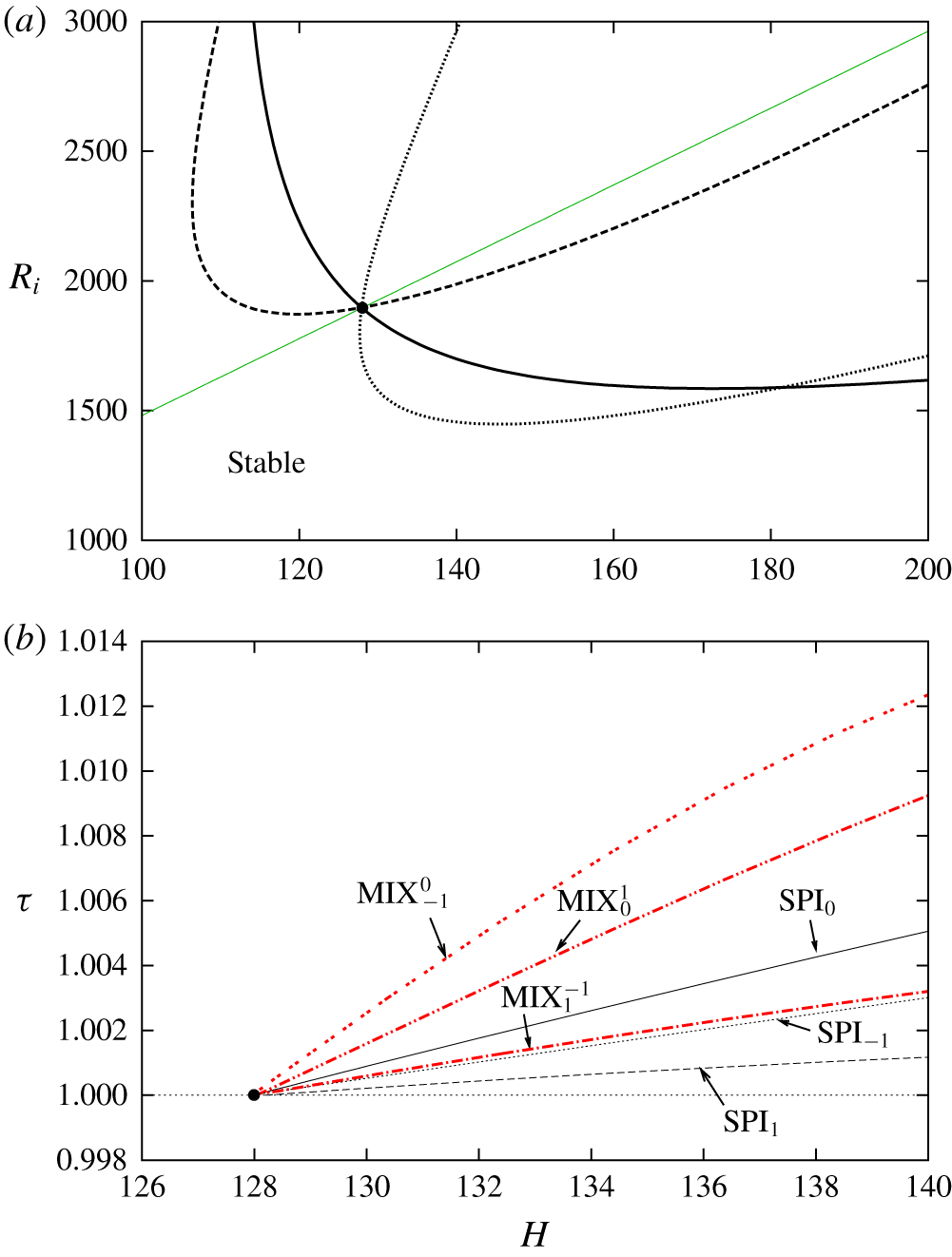
 $\unicode[STIX]{x1D6FF}=0.0413$ there is a point where all three modes become neutral simultaneously, as clearly shown in figure 3.
Linear stability analysis and continuation of bifurcated nonlinear solution branches in the anticyclonic regime for  $(\unicode[STIX]{x1D6FF},\unicode[STIX]{x1D702})=(0.0413,0.5)$. (a) Neutral stability curves along the line
 $R_{o}=0.26R_{i}/\unicode[STIX]{x1D702}$ (black curves) for modes
 $m=0$ (solid) and
 $m=\pm 1$ (dashed for
 $+1$, dotted for
 $-1$). Wavenumber
 $k$ is the one that maximises growth rate. The black circle indicates the triple critical point at
 $(H,R_{i})=(128,1896)$. (b) Bifurcation diagram along
 $R_{i}=(1896/128)H$ (green line in panel a). The black circle corresponds again to the triple-critical point, whence three spiral (
 $\text{SPI}_{0}$,
 $\text{SPI}_{\pm 1}$; solid, dashed and dotted black lines) and three mixed (
 $\text{MIX}_{1}^{-1}$,
 $\text{MIX}_{1}^{0}$,
 $\text{MIX}_{0}^{-1}$; solid, dashed and dotted red lines) modes are issued.

For the sake of clarity, we shall focus on the computation and continuation of nonlinear solutions along the straight line across parameter space  $R_{i}=(1896/128)H$ (green solid line in figure 3a) that passes through the triple critical point at
 $(H,R_{i})=(128,1896)$. Figure 3(b) depicts the bifurcation diagram corresponding to the six different nonlinear solution branches, as characterised by torque as a function of the Hartmann number. At the triple critical point, the three eigenmodes,
 $(m,k)=(0,5.672)$,
 $(m,k)=(1,4.672)$ and
 $(m,k)=(-1,2.818)$, become neutral simultaneously. As anticipated by weakly nonlinear analysis, bifurcation of various mixed modes is therefore expected. The Newton method described in § 2 does indeed converge to one or another of the nonlinear pure- or mixed-mode solutions when a suitably weighted superposition of the three neutral eigenmodes is taken as an initial guess. Solutions have initially been computed in this way in the close neighbourhood of the triple critical point and then continued as a function of
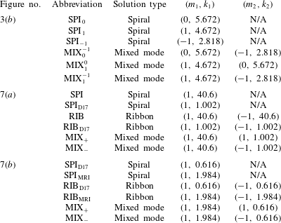
 $H$ using either natural or pseudo-arclength continuation algorithms. Three of the solution branches, converged from single-mode initial guesses fed into the Newton method, correspond to helically invariant travelling spiral waves (black curves in figure 3b). These solutions we have dubbed as
 $\text{SPI}_{m}$, with the subscript
 $m$ (solid black line for
 $m=0$, dashed for
 $m=1$, dotted for
 $m=-1$) denoting the azimuthal wavenumber of the mode (see table 1). All three branches bifurcate supercritically from the base laminar flow. Since these solutions can be computed in the usual rectangular domain using regular coordinates
 $(\unicode[STIX]{x1D703},z)$, we omit a detailed analysis.
Abbreviations used to describe the various nonlinear solution branches. Note that  $\text{SPI}_{0}$ is a zero-pitch spiral, and therefore a toroidal-vortex-pair solution.

Suitable proportions of the weights applied to the critical eigenmodes in generating the initial seeds for the Newton method have allowed computation of all three possible mixed-mode nonlinear solution branches (red curves in figure 3b). These mixed modes have been labelled as  $\text{MIX}_{m_{1}}^{m_{2}}$, with the sub- and superscripts representing the azimuthal wavenumber of the two interacting modes, and duly reported in table 1. As mentioned earlier, these mixed modes can only be identified using an appropriate annular-parallelogram domain, as the superposition of the two modes does not fit any rectangular domain of affordable size.
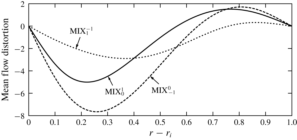
Azimuthal mean flow distortion ( $\overline{v}-v_{b}$) of the three different mixed modes shown in figure 3(b) for
 $H=140$, and
 $(R_{i},R_{o})\approx (2074,1078)$.

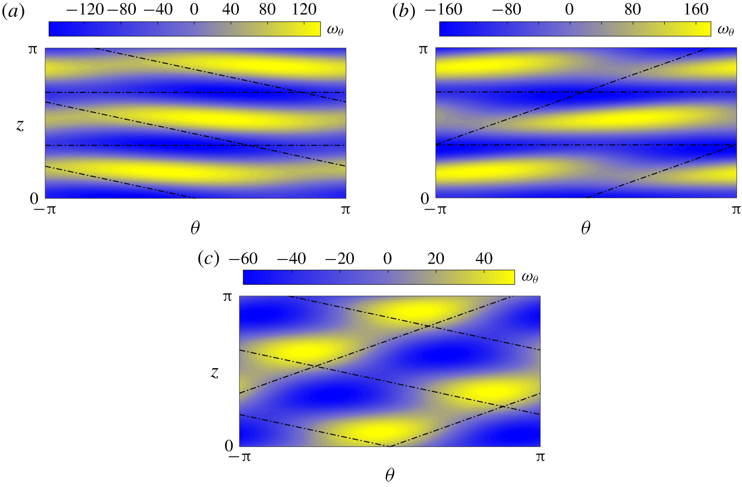
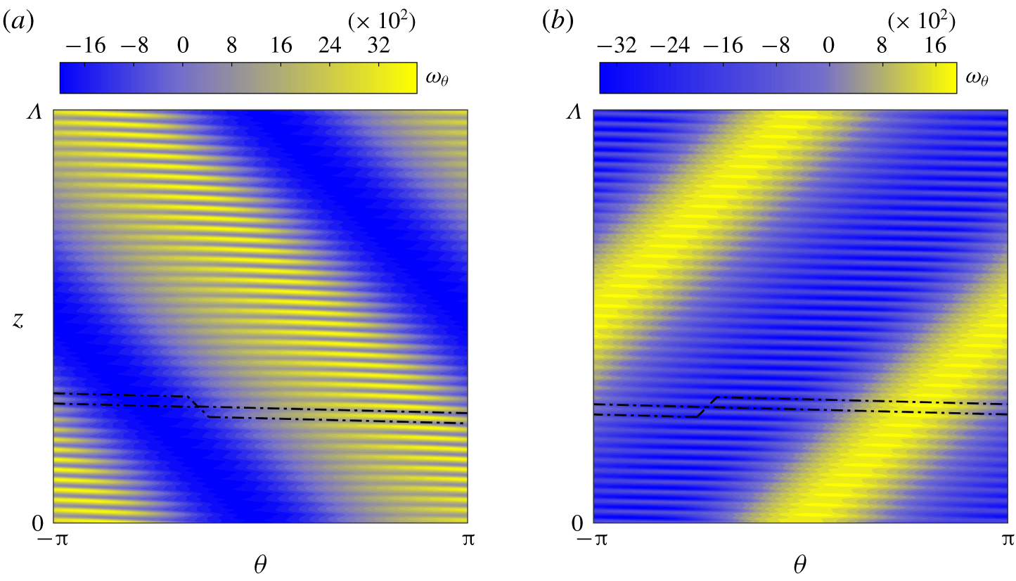
Colour maps of the total azimuthal vorticity ( $\unicode[STIX]{x1D714}_{\unicode[STIX]{x1D703}}=\unicode[STIX]{x2202}_{z}u-\unicode[STIX]{x2202}_{r}w$) distribution at the mid-radial-plane
 $r=r_{i}+0.5$ of the three mixed-mode MRI solutions: (a)
 $\text{MIX}_{1}^{0}$, (b)
 $\text{MIX}_{-1}^{0}$ and (c)
 $\text{MIX}_{-1}^{1}$.

All three mixed-mode branches bifurcate supercritically. A very remarkable feature of these mixed modes is that some of them have larger torque than the spirals. This aspect is of special relevance to the study of astrophysical accretion disks, as it is a paramount requirement for the large outward angular momentum flux that is believed to be the key to the observed rate of inward mass accretion. The  $\text{MIX}_{-1}^{0}$ mode possesses the largest torque of all mixed modes, as is also clear from the azimuthal mean flow distortion shown in figure 4 for
 $H=140$,
 $(R_{i},R_{o})\approx (2074,1078)$. Figure 5 shows the corresponding total azimuthal vorticity distribution of the three mixed modes, represented through
 $\unicode[STIX]{x1D703}$–
 $z$ plane colour maps at mid-gap
 $r=r_{i}+0.5$. As expected, mode
 $\text{MIX}_{-1}^{0}$ has the strongest flow field perturbation, clearly reflected in the colour bar range of the panels. The visualisations shown in figure 5(a) and (b) for
 $\text{MIX}_{0}^{1}$ and
 $\text{MIX}_{-1}^{0}$, respectively, are reminiscent of wavy Taylor vortex flow (see e.g. Andereck et al. (Reference Andereck, Liu and Swinney1986)) except that the patterns are tilted and wavy vortex pairs accumulate an azimuthal phase shift as they pile up in the axial direction. The reason for this is that one of its constituents is a zero-pitch spiral, which corresponds to a toroidal-vortex-pair solution much like Taylor vortices, while the superposition of a spiral mode generates the tilted azimuthal modulation. Meanwhile, the structure of the
 $\text{MIX}_{1}^{-1}$ mode shown in figure 5(c) is evocative of the wavy spiral solution found in the hydrodynamic studies by Altmeyer & Hoffmann (Reference Altmeyer and Hoffmann2010) and Deguchi & Altmeyer (Reference Deguchi and Altmeyer2013).
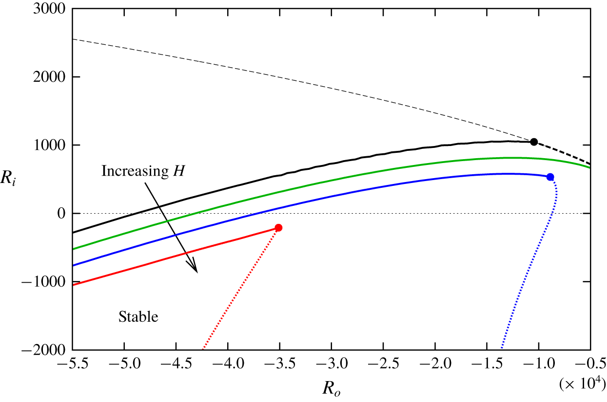
Neutral curves for  $H=0,40,60,84$ (black, green, blue, red, respectively) and
 $\unicode[STIX]{x1D702}=0.1$. The wavenumber pairs
 $(k,m)$ are optimised to detect the most unstable eigenvalue. The neutral curve for the classical non-axisymmetric hydrodynamic mode (dashed black) is shown alongside those for the D17 mode (solid black) and the MRI mode (dotted). While
 $m$ is large and obeys the asymptotic result by Deguchi (Reference Deguchi2016) for the classical neutral curve, the D17 and MRI neutral curves have typically
 $m=\pm 1$. Bicritical points, where direct bifurcation of mixed-mode solution branches are expected, are indicated with filled circles.

4 From counter-rotation to the cyclonic super-rotation regime
In this section we focus our attention on the bifurcations arising on the left half-plane of figure 1, as some of the instabilities carry on to the super-rotation regime. For  $\unicode[STIX]{x1D702}=0.1$, figure 6 outlines the neutral curves obtained from linear stability analyses corresponding to different levels of magnetisation. We begin our analysis by first focusing on the purely hydrodynamic case in the absence of magnetic effects. Shown in figure 6 are the classical neutral curve (dashed black) alongside the neutral curve for the D17 mode (solid black), recently discovered by Deguchi (Reference Deguchi2017) through linear stability analysis.
Along the classical boundary, the critical value of  $R_{i}$ increases with
 $|R_{o}|$, which is consistent with extensive numerical evidence as well as physical insights and the large-Reynolds-number formal asymptotic result (Esser & Grossmann Reference Esser and Grossmann1996; Deguchi Reference Deguchi2016; Grossmann et al. Reference Grossmann, Lohse and Sun2016). As a consequence, the neutral curve, which corresponds to a non-axisymmetric leading mode with large
 $m$ (a spiral), cannot be continued across the line
 $R_{i}=0$ into the super-rotation regime.
In contrast, the neutral curve for the D17 mode, typically with  $m=\pm 1$, does indeed extend to the cyclonic super-rotation regime. The reason for choosing such a low value of the radius ratio (
 $\unicode[STIX]{x1D702}=0.1$) follows from the observation that the curve shifts to very high counter-rotation rates as
 $\unicode[STIX]{x1D702}$ is increased and narrower gaps are considered. For instance, taking
 $R_{i}=0$ and
 $\unicode[STIX]{x1D702}=5/7$ pushes the critical
 $R_{o}$ value to
 $O(10^{7})$, whereas for
 $\unicode[STIX]{x1D702}=0.1$ it remains within order
 $O(10^{4})$. In figure 6, the classical stability threshold (dashed black) and the new one set by the neutral curve of the D17 mode (solid black) meet at a bicritical point (black filled circle) located at
 $(R_{i},R_{o})\approx (1045,-10\,434)$, with associated critical wavenumbers
 $(m_{1},k_{1})=(1,40.6)$ and
 $(m_{2},k_{2})=(1,1.102)$, respectively. The critical axial wavenumbers
 $k_{1}$ and
 $k_{2}$ associated with either mode differ significantly, which explains why the latter, mode D17, escaped detection for so long. The asymptotic theory provided by Deguchi (Reference Deguchi2016) formally proved that the critical axial wavenumber of the classical mode gets asymptotically large for increasing Reynolds numbers, while that for the D17 mode seems to be insensitive to Reynolds-number variations.
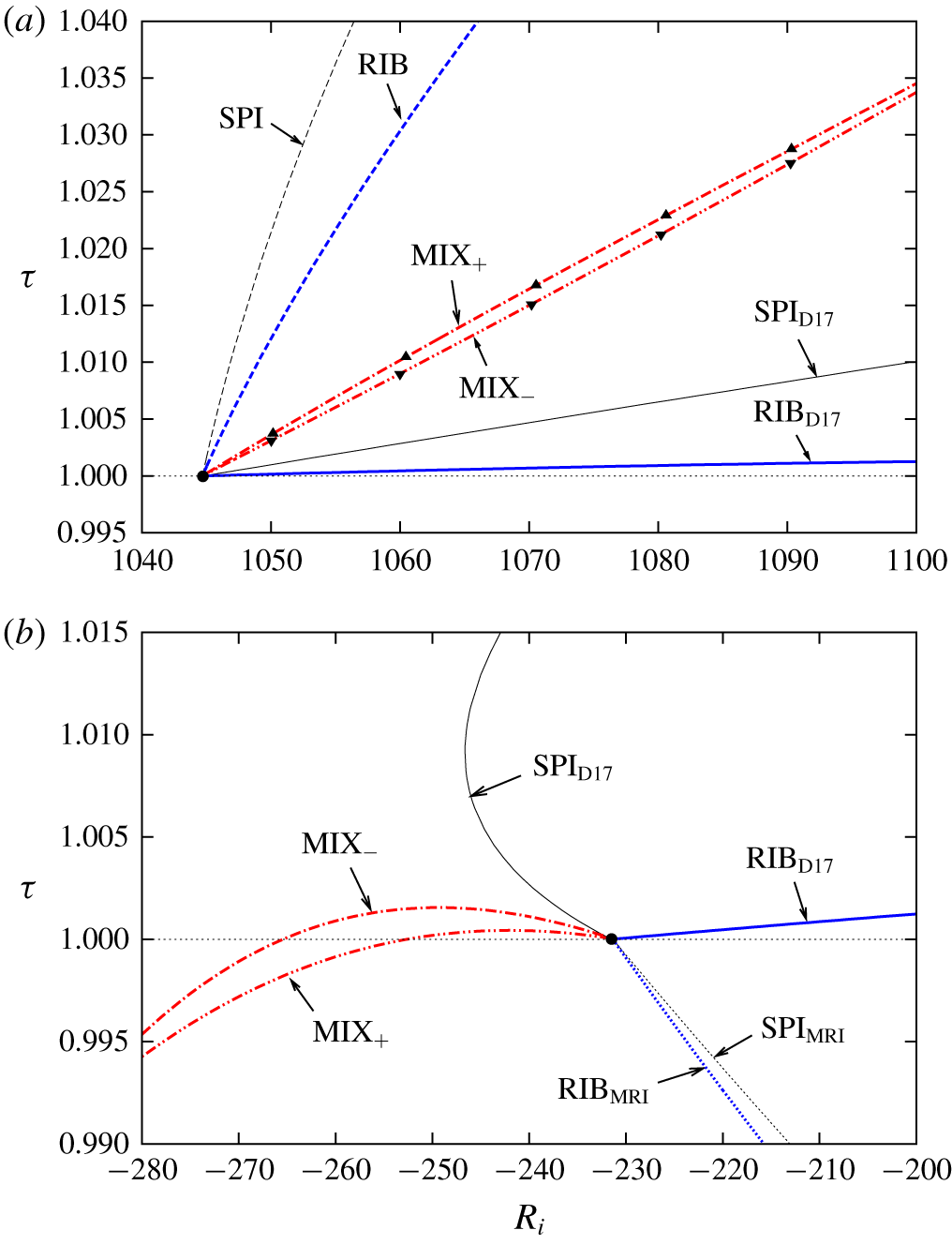
Bifurcation diagrams of spirals, ribbons and mixed nonlinear modes in super- and counter-rotation configurations. (a) Purely hydrodynamic case, in counter-rotation with  $R_{o}=-10\,434$ and
 $H=0$. The black circle indicates the linear bicritical point at
 $R_{i}=1045$. A bunch of mixed-mode solutions computed with the alternative Petrov–Galerkin code are marked with triangles. (b) Magnetised case in the super-rotation regime with
 $R_{o}=-35\,150$ and
 $H=84$. The bicritical point at
 $R_{i}=-231.5$ is indicated with a filled black circle.

The various nonlinear solution branches that bifurcate from the bicritical point (black filled circle in figure 6) are shown in figure 7(a). All branches bifurcate supercritically. The black curves correspond to the spiral solutions for the classical spiral mode (SPI, dashed) and the D17 mode ( $\text{SPI}_{\text{D}17}$, solid). The structure of the single-mode solutions, the nonlinear spirals, are qualitatively identical to the linear neutral mode (see Deguchi Reference Deguchi2017). Since the system is symmetric with respect to axial reflections (
 $z\rightarrow -z$), spiral modes become neutral in pairs, with exactly opposite pitch. As a result, there are actually four modes that simultaneously become neutral at the linear bicritical point (the black filled circle in figure 7a). Consequently, there exist six mixed modes arising from all possible combinations of modes taken in pairs. Two of them merely correspond to ribbon solutions (blue curves in figure 7a), labelled as RIB (dashed, SPI–SPI interaction) and
 $\text{RIB}_{\text{D}17}$ (solid,
 $\text{SPI}_{\text{D}17}$–
 $\text{SPI}_{\text{D}17}$ interaction), and listed in table 1. While ribbon solutions can be computed in a rectangular domain, all other mixed modes require the use of the annular-parallelogram domain. In fact, only two of the four remaining modes actually require computation, as the other two can be easily obtained from simple
 $z$ reflection and, since the torque is invariant under this symmetry operation, the solution branches are exactly coincident. The branches corresponding to these mixed-mode solutions are shown in red in figure 7(a). The branch labelled as
 $\text{MIX}_{+}$ originates from the interaction of two modes with pitches of the same sign, while the one labelled
 $\text{MIX}_{-}$ arises from the nonlinear coupling of modes with opposite sign, as reported in table 1.
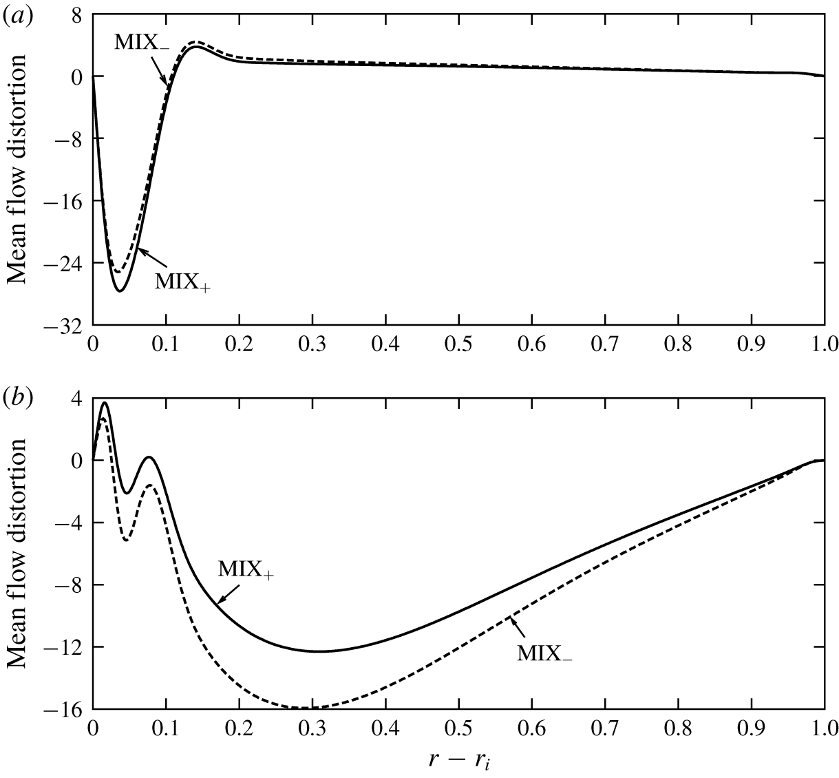
All hydrodynamic results reported in this work and initially computed with a code based on the hydromagnetic-potential formulation (2.13) have been reproduced using the independently developed solenoidal Petrov–Galerkin parallelogram formulation (2.20). A few nonlinear solutions at selected values of the parameters have been chosen and indicated with triangles in figure 7(a) to convey the excellent qualitative agreement between the two methods employed for the computations. Quantitative comparison shows that the torque discrepancy stays below  $0.06\,\%$ for all the purely hydrodynamic nonlinear mixed-mode solutions computed. Figure 8(a) represents the azimuthal mean flow distortion for the mixed modes at
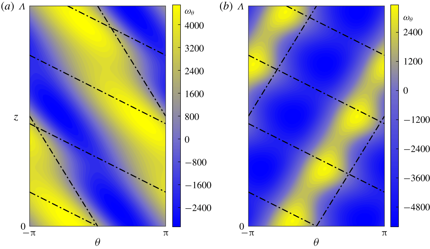
 $(R_{i},R_{o})=(1100,-10\,434)$. The distortion is the most significant in the vicinity of the inner cylinder, which indicates that the perturbation is strongest in this region. For the same values of the parameters, figure 9 shows azimuthal vorticity colour maps for both mixed modes on an unwrapped radial plane at
 $r=r_{i}+0.05$. The observed flow structure is very different from any of the mixed-mode solutions reported by Deguchi & Altmeyer (Reference Deguchi and Altmeyer2013). The observed small–large scale interaction reminds one of the stripe pattern that is characteristic of intermittent spiral turbulence (Dong Reference Dong2009; Meseguer et al. Reference Meseguer, Mellibovsky, Avila and Marques2009). While the Reynolds numbers and the gap are too large to claim there exists any relation between the mixed modes presented here and spiral turbulence, the similarity of the patterns indicates that spiral turbulence might indeed be supported by mixed-mode solutions of very different pitches as the ones investigated here in a completely different setting.


Visualisation of the total azimuthal vorticity ( $\unicode[STIX]{x1D714}_{\unicode[STIX]{x1D703}}=\unicode[STIX]{x2202}_{z}u-\unicode[STIX]{x2202}_{r}w$) at
 $r=r_{i}+0.05$ for the purely hydrodynamic mixed-mode solutions at
 $R_{i}=1100$ in figure 7(a). Here
 $\unicode[STIX]{x1D6EC}=2\unicode[STIX]{x03C0}/1.002\approx 6.27$: (a)
 $\text{MIX}_{-}$ and (b)
 $\text{MIX}_{+}$. The corresponding mean flow distortion was shown in figure 8(a).

Now we turn our attention to the magnetised problem, where we will impose an external magnetic field with a strictly azimuthal orientation. For the MRI studies in an annulus, the azimuthal base magnetic field is typically the weighted superposition of  $r^{-1}$ and
 $r$ components. The respective coefficients can be tuned by an appropriate uniform current imposed within the inner and outer cylinders. Rüdiger et al. (Reference Rüdiger, Schultz, Gellert and Stefani2016, Reference Rüdiger, Schultz, Gellert and Stefani2018b) considered two extreme cases:
 $B_{b}(r)\propto r^{-1}$ (i.e. there is no current between the cylinders) and
 $B_{b}(r)\propto r$ (i.e. the axial current is homogeneous between the cylinders). The latter also has the alternative name
 $z$ pinch, and is known to become unstable for sufficiently large Hartmann number even with both cylinders at rest (Tayler Reference Tayler1957). As the Taylor instability does not exist for the current-free case, the behaviour of the neutral curve for small Reynolds numbers must necessarily be quite different from that for the homogeneous current case. Rüdiger et al. (Reference Rüdiger, Schultz, Gellert and Stefani2016, Reference Rüdiger, Schultz, Gellert and Stefani2018b) found that, for
 $\unicode[STIX]{x1D702}\gtrsim 0.8$, the neutral curves behave qualitatively alike in both cases when Reynolds numbers are moderately large, thereby suggesting that super-AMRI is rather insensitive to the choice of the azimuthal magnetic field profile.
We have confirmed that the D17 mode is stabilised by both the current-free and the  $z$-pinch cases. Nonetheless, when the two azimuthal magnetic field components exist simultaneously, the D17 mode can be destabilised, as clearly illustrated by the behaviour of the neutral stability curves in figure 6. Here the specific magnetic field profile used is
 $$\begin{eqnarray}B_{b}(r)=\frac{r_{i}}{r}-\frac{r}{r_{o}},\quad C_{b}(r)=0.\end{eqnarray}$$
Although the arguments by Rüdiger et al. (Reference Rüdiger, Schultz, Gellert and Stefani2016, Reference Rüdiger, Schultz, Gellert and Stefani2018b) for the current-free case may not be applicable to the large gap  $\unicode[STIX]{x1D702}=0.1$ we tackle here, an MRI does indeed arise when a current is considered. This phenomenon had already been anticipated by a locally periodic approach (see Liu et al. Reference Liu, Goodman, Herron and Ji2006; Kirillov, Stefani & Fukumoto Reference Kirillov, Stefani and Fukumoto2014), but the nature of the method used renders the approximation rather crude in view of the not-so-large critical wavenumbers we encounter here. As the Hartmann number is increased, the super-AMRI mode eventually takes over the classical mode, and hence changes the character of the bicritical point. In view of figure 6 at
 $H=60$, the double critical point is already the result of the interaction of the D17 and the super-AMRI modes. The base flow remains stable within the region bounded by their respective stability thresholds. Along the combined neutral curve, the critical axial wavenumber experiences a discontinuous leap across the bicritical point, whence it must be inferred that the two instability mechanisms are indeed distinct. By further increasing the Hartmann number, the bicritical point moves towards and eventually crosses into the super-rotation regime. We have determined that the bicritical point crosses the
 $R_{i}=0$ line somewhere between
 $H=80$ and
 $H=84$.
The nonlinear solution branches issued from the bicritical point  $(R_{i},R_{o})\approx (-231.5,-35\,150)$ at
 $H=84$ have been computed in the same way they were for the strictly hydrodynamic case studied above. The critical wavenumbers of the magnetised D17 mode at this point are
 $(m,k)=(1,0.616)$, while those for the super-AMRI modes are
 $(m,k)=(1,1.984)$, which entails flow structures of similar sizes. The bifurcation diagram of figure 7(b) has been obtained by varying
 $R_{i}$ at constant
 $R_{o}$. To the right (left) of the linear critical point, the base flow is unstable to the D17 (super-AMRI) mode. The imposed azimuthal magnetic field does not break any of the inherent symmetries of the hydrodynamic Taylor–Couette system so that, as in the hydrodynamic case discussed above, there still arise two spirals (along with their mirror images), two ribbons and two mixed modes (and mirror images). See table 1 for an account of all modes. Both nonlinear spiral branches (black curves: solid for
 $\text{SPI}_{\text{D}17}$, dashed for
 $\text{SPI}_{\text{MRI}}$) bifurcate subcritically, in the sense that they exist when the corresponding linear mode is stable. However, this is only true while their amplitude remains small, and the branch associated with the D17 mode turns back in a saddle-node bifurcation towards lower
 $|R_{i}|$. The
 $\text{RIB}_{\text{D}17}$ (solid blue) and
 $\text{RIB}_{\text{MRI}}$ (dashed blue) solution branches both exist to the right of the critical point (blue curves in figure 7b).
We note in passing that the super-AMRI-type ribbon solutions found by Rüdiger et al. (Reference Rüdiger, Schultz, Gellert and Stefani2016) were shown to be stable by direct numerical simulation. The mixed-mode solution branches (red curves) come in two types, namely  $\text{MIX}_{+}$ and
 $\text{MIX}_{-}$, depending on whether the interacting modes have the same or opposite pitch, respectively. Unlike all other solution branches issued from the bicritical point, these extend to large
 $|R_{i}|$, and may thus govern the dynamics within the region of the super-rotation regime closest to solid-body rotation.
As is clear from figure 7(b), the nonlinear solution branches associated with the super-AMRI instability have the unforeseen property that the torque is reduced with respect to the laminar base value. The dependence of torque on Reynolds number associated with the two mixed modes follows very similar trends. The torque initially grows away from the bifurcation point as the branches dive deep into the super-rotation regime, but the trend is soon reversed and the torque eventually drops below laminar values.
The reason for torque reduction can be understood from the energy balance, since torque corresponds to one of the energy input mechanisms. The perturbation energy budget can be found by integrating  . For travelling-wave-type solutions, perturbation energy must be time-independent and thus the balance
 $$\begin{eqnarray}\left\langle r\left(\frac{v_{b}}{r}\right)^{\prime }\widetilde{u}\widetilde{v}\right\rangle -H^{2}\langle r^{-1}(rB_{b})^{\prime }(\widetilde{a}\widetilde{v}-\widetilde{u}\widetilde{b})\rangle =\langle \widetilde{\boldsymbol{v}}\boldsymbol{\cdot }\unicode[STIX]{x1D6FB}^{2}\widetilde{\boldsymbol{v}}\rangle +H^{2}\langle \widetilde{\boldsymbol{b}}\boldsymbol{\cdot }\unicode[STIX]{x1D6FB}^{2}\widetilde{\boldsymbol{b}}\rangle\end{eqnarray}$$
should be satisfied. Here the angle brackets denote integration over the annular-parallelogram domain. The first terms on the right- and left-hand sides are related to the torque, since integration of  yields
 $$\begin{eqnarray}-\left\langle r\left(\frac{v_{b}}{r}\right)^{\prime }\widetilde{u}\widetilde{v}\right\rangle =\langle v_{b}\boldsymbol{e}_{\unicode[STIX]{x1D703}}\boldsymbol{\cdot }\unicode[STIX]{x1D6FB}^{2}\widetilde{\boldsymbol{v}}\rangle\end{eqnarray}$$
and integration by parts of the first term on the right-hand side results in
 $$\begin{eqnarray}\langle \boldsymbol{v}\boldsymbol{\cdot }\unicode[STIX]{x1D6FB}^{2}\boldsymbol{v}\rangle =(r_{o}^{-1}R_{o}-r_{i}^{-1}R_{i})T-\langle |\unicode[STIX]{x1D735}\boldsymbol{v}|^{2}\rangle .\end{eqnarray}$$
The energy balance equation (4.2) then becomes
 $$\begin{eqnarray}-H^{2}\langle \widetilde{\boldsymbol{b}}\boldsymbol{\cdot }\unicode[STIX]{x1D6FB}^{2}\widetilde{\boldsymbol{b}}\rangle -H^{2}\langle r^{-1}(rB_{b})^{\prime }(\widetilde{a}\widetilde{v}-\widetilde{u}\widetilde{b})\rangle =(r_{o}^{-1}R_{o}-r_{i}^{-1}R_{i})T-\langle |\unicode[STIX]{x1D735}\boldsymbol{v}|^{2}\rangle .\end{eqnarray}$$
Showing that torque cannot decrease below the laminar value for purely hydrodynamic Taylor–Couette flow is a straightforward exercise, because the terms on the left-hand side are identically zero. The calculus of variations can then be used to prove that the minimum value of the functional  $\boldsymbol{F}(\boldsymbol{v})=\langle |\unicode[STIX]{x1D735}\boldsymbol{v}|^{2}\rangle$ under the divergence-free constraint for
 $\boldsymbol{v}$ is realised by the solution to the Stokes equation (see e.g. Doering & Gibbon Reference Doering and Gibbon1995), namely the laminar Couette solution. Imposing
 $\langle |\unicode[STIX]{x1D735}\boldsymbol{v}|^{2}\rangle \geqslant \langle |\unicode[STIX]{x1D735}\boldsymbol{v}_{b}|^{2}\rangle =(r_{o}^{-1}R_{o}-r_{i}^{-1}R_{i})T_{b}$ on (4.4) demands that
 $\unicode[STIX]{x1D70F}\geqslant 1$ for the purely hydrodynamic case.
Moreover, the balance equation further leads to the conclusion that torque reduction cannot occur at all if the base magnetic field is current-free, as this entails that the second term on the left-hand side of (4.5) is absent. The proof is again straightforward, as integration by parts shows that  $-H^{2}\langle \widetilde{\boldsymbol{b}}\boldsymbol{\cdot }\unicode[STIX]{x1D6FB}^{2}\widetilde{\boldsymbol{b}}\rangle$ is positive definite. The resulting inequality,
 $$\begin{eqnarray}\displaystyle (r_{o}^{-1}R_{o}-r_{i}^{-1}R_{i})T & {\geqslant} & \displaystyle (r_{o}^{-1}R_{o}-r_{i}^{-1}R_{i})T+H^{2}\langle \widetilde{\boldsymbol{b}}\boldsymbol{\cdot }\unicode[STIX]{x1D6FB}^{2}\widetilde{\boldsymbol{b}}\rangle =\langle |\unicode[STIX]{x1D735}\boldsymbol{v}|^{2}\rangle \nonumber\\ \displaystyle & {\geqslant} & \displaystyle (r_{o}^{-1}R_{o}-r_{i}^{-1}R_{i})T_{b},\end{eqnarray}$$
yields again  $\unicode[STIX]{x1D70F}\geqslant 1$. This outlines the necessity of a base current field if torque reduction is to be observed.
As seen in figure 7(b), the torque reduction is stronger for the  $\text{MIX}_{+}$ mode, reflecting the fact that the perturbation is slightly larger for that mode. This is evidenced by figure 8(b), where the azimuthal mean flow distortion across the gap is plotted at
 $R_{i}=-280$. The oscillatory modulation of the flow near the inner cylinder is responsible for the torque reduction and is driven by the vortex structure near the inner cylinder, as shown in the
 $\unicode[STIX]{x1D703}$–
 $z$ sections of figure 10. Here again we choose
 $r=r_{i}+0.05$, very close to the inner cylinder, as the reference radius. As expected, the perturbation of the
 $\text{MIX}_{+}$ mode has larger amplitude than that for the
 $\text{MIX}_{-}$ mode. The flow patterns are similar to those of the wavy spiral computed by Altmeyer & Hoffmann (Reference Altmeyer and Hoffmann2010) and Deguchi & Altmeyer (Reference Deguchi and Altmeyer2013), because the critical wavenumbers of the interacting modes are of comparable size.
Visualisation of the total azimuthal vorticity ( $\unicode[STIX]{x1D714}_{\unicode[STIX]{x1D703}}=\unicode[STIX]{x2202}_{z}u-\unicode[STIX]{x2202}_{r}w$) at
 $r=r_{i}+0.05$ for the magnetised mixed-mode solutions at
 $R_{i}=-280$ in figure 7(b). Here
 $\unicode[STIX]{x1D6EC}=2\unicode[STIX]{x03C0}/0.616\approx 10.2$: (a)
 $\text{MIX}_{-}$ and (b)
 $\text{MIX}_{+}$. The corresponding mean flow distortion was shown in figure 8(b).

5 Conclusions
We have investigated nonlinear mode competition in MHD Taylor–Couette flow subject to predominantly azimuthal magnetic fields. For this purpose, a Newton solver devised by Deguchi & Altmeyer (Reference Deguchi and Altmeyer2013) for the Navier–Stokes equations in annular-parallelogram domains has been extended for its application to the inductionless limit of the MHD equations.
For the anticyclonic regime (see figure 1), a suitably adjusted weak axial magnetic field in addition to the azimuthal field stimulates linear instability modes with  $m=-1,0,1$, as anticipated by Hollerbach et al. (Reference Hollerbach, Teeluck and Rüdiger2010). Consistent with their results, we find particularly rich nonlinear dynamics for
 $\unicode[STIX]{x1D6FF}\simeq 0.04$. In § 3, we identified that there is a triple critical point involving all three modes for
 $\unicode[STIX]{x1D6FF}\approx 0.0413$. We have tracked the three nonlinear mixed-mode solution branches that bifurcate simultaneously at the triple critical point using the purposely devised Newton solver and arclength continuation. Some of the mixed-mode solutions possess a larger angular momentum transport (they require application of higher driving torque to keep the cylinders rotating) than the single-mode solutions they result from. This increased transport of angular momentum makes these mixed-mode solutions an interesting target for future study, as they might be relevant in astrophysical flows involving accretion disks. In particular, a better understanding of what their role might be in the nonlinear dynamics of such flows will require direct numerical simulations and experiments such as those by PROMISE (Rüdiger et al. Reference Rüdiger, Hollerbach, Stefani, Gundrum, Gerbeth and Rosner2006; Stefani et al. Reference Stefani, Gundrum, Gerbeth, Rüdiger, Schultz, Szklarski and Hollerbach2006, Reference Stefani, Gundrum, Gerbeth, Rüdiger, Szklarski and Hollerbach2007).
In § 4, we have studied mode competition involving the D17 mode. In the purely hydrodynamic case, there is a point where both the classical spiral mode and the D17 mode become neutral simultaneously. This bicritical point lies within the counter-rotation regime (see figure 1). The corresponding mixed-mode solutions consist of an interesting stripe pattern where the small-scale classical spirals are modulated by the larger-scale structure of the D17 mode. All purely hydrodynamic results presented here are in excellent agreement with analogous computations done with an independently developed Petrov–Galerkin code devised by Meseguer et al. (Reference Meseguer, Avila, Mellibovsky and Marques2007) and presently extended to allow computation of mixed-mode travelling–rotating wave solutions in annular-parallelogram domains. This code is better suited for the study of large-scale pattern formation in Taylor–Couette flow and includes not only a travelling–rotating wave Newton–Krylov matrix-free solver (thus being capable of handling a much larger number of degrees of freedom), but also stability analysis, a solver for modulated travelling–rotating waves and pseudo-arclength continuation of solution branches adapted from Mellibovsky & Meseguer (Reference Mellibovsky and Meseguer2015), and also direct numerical simulation. Details of this second code and its adaptation to annular-parallelogram domains will be presented in our future work on the study of large-scale pattern formation in Taylor–Couette flow. The intricacies of the method reach beyond the scope of the present study.
The application of an external azimuthal magnetic field alters the picture obtained in the purely hydrodynamic case completely. The non-axisymmetric super-AMRI mode found by Rüdiger et al. (Reference Rüdiger, Schultz, Gellert and Stefani2016, Reference Rüdiger, Gellert, Hollerbach, Schultz and Stefani2018a,Reference Rüdiger, Schultz, Gellert and Stefanib) appears at moderate Hartmann numbers and eventually outweighs the classical mode for sufficiently strong magnetic fields. We clearly show that the mechanisms behind the magnetised D17 mode and the super-AMRI mode are distinct. Destabilisation of the D17 mode occurs for a given external magnetic field profile (4.1). As a result, an increase of the Hartmann number gradually shifts the bicritical point at which both modes are simultaneously destabilised towards the super-rotation regime. This fact renders this mode interaction interesting from an astrophysical point of view. Several nonlinear solution branches are issued from the bicritical point in both  $R_{i}$ directions at fixed
 $R_{o}$. While spirals and ribbons return towards the counter-rotation regime, the mixed-mode solution branches plunge deep into the super-rotation regime.
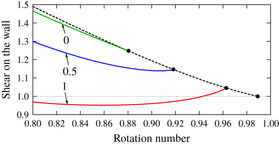
The solutions computed in § 4 show how the complex interplay between the nonlinear shear–Coriolis and the magneto-rotational instabilities can sometimes lead to torques lower than that of the base flow. This surprising result is in sharp contrast with what is typically assumed in purely hydrodynamic shear-flow studies, where nonlinearity is known to invariably enhance angular momentum transport. This torque reduction occurs even for finite  $P_{m}$ and sub-rotation of the cylinders; see appendix B. In view of this result, torque reduction might be a generic property of MHD flows in the presence of shear and Coriolis forces. A particularly interesting potential application of this phenomenon would be to design control strategies to reduce drag on the curved boundary layers by imposing suitable magnetic fields.
We have analysed the D17/super-AMRI mode interaction for a large gap  $\unicode[STIX]{x1D702}=0.1$. Interesting as it would be, we have not attempted here to track these modes to smaller annulus gaps in the order
 $\unicode[STIX]{x1D702}\sim 0.8$ and test the robustness of the coalescence point of both instabilities. The extremely large Reynolds numbers at which the D17 mode bifurcates in the narrow annulus case renders the task overly demanding from a computational point of view, if not altogether unaffordable.
Imposing more intense helical magnetic fields might also be an appealing topic for future research. The two axisymmetric super-HMRI modes found recently by Mamatsashvili et al. (Reference Mamatsashvili, Stefani, Hollerbach and Rüdiger2019), in combination with some of the modes studied here, may also yield rich interaction patterns worth exploring. While their type 2 super-HMRI mode belongs to the class of MRI requiring induction together with SMRI, the type 1 super-HMRI mode is inductionless and might therefore coexist with the super-AMRI mode and interact nonlinearly. Both types of super-HMRI modes might of course interact with the D17 mode. For HMRI, the further consideration of current in the fluid brings about even richer instability phenomena as anticipated by a locally periodic approach (Liu et al. Reference Liu, Goodman, Herron and Ji2006; Kirillov & Stefani Reference Kirillov and Stefani2013; Kirillov et al. Reference Kirillov, Stefani and Fukumoto2014). The interaction of short-wavelength modes found using the locally periodic approach with longer-wavelength modes such as D17 or super-AMRI modes would generate band-like patterns much as those in figure 9.
Acknowledgements
K.D.’s research was supported by Australian Research Council Discovery Early Career Researcher Award DE170100171. The research of R.A., F.M. and A.M. was supported by the Spanish MINECO grants FIS2016-77849-R and FIS2017-85794-P and the Generalitat de Catalunya grant 2017-SGR-785. We gratefully acknowledge insightful comments and suggestions made by Professor R. Hollerbach during the review process.
Declaration of interests
The authors report no conflict of interest.
Appendix A. Basis function for the magnetic potentials
Following Roberts (Reference Roberts1964), we first determine the magnetic field for the outer zones  $r<r_{i}$ and
 $r>r_{o}$. Within the perfectly insulating walls, the magnetic field must have a potential
 $\unicode[STIX]{x1D711}$ because there is no current:
 $$\begin{eqnarray}\widetilde{a}=\unicode[STIX]{x1D711}_{r},\quad \widetilde{b}=r^{-1}\unicode[STIX]{x1D711}_{\unicode[STIX]{x1D703}},\quad \widetilde{c}=\unicode[STIX]{x1D711}_{z}.\end{eqnarray}$$
Since the magnetic field is solenoidal, the outer potential must satisfy Laplace’s equation. Using the expansion
 $$\begin{eqnarray}\unicode[STIX]{x1D711}=\mathop{\sum }_{n_{1},n_{2}}\widehat{\unicode[STIX]{x1D711}}_{n_{1}n_{2}}(r)\text{e}^{\text{i}(n_{1}\unicode[STIX]{x1D709}_{1}+n_{2}\unicode[STIX]{x1D709}_{2})},\end{eqnarray}$$
it is easy to find that the solution  $\widehat{\unicode[STIX]{x1D711}}_{n_{1}n_{2}}(r)$ can be written down using the modified Bessel functions of the first and second kinds,
 $\text{I}_{\unicode[STIX]{x1D708}}(x)$ and
 $\text{K}_{\unicode[STIX]{x1D708}}(x)$, both of which satisfy
 $x^{2}f^{\prime \prime }+xf^{\prime }-(x^{2}+\unicode[STIX]{x1D708}^{2})f=0$. The requirement that the potential is analytic at
 $r=0$ determines the solution for
 $r<r_{i}$ as
 $$\begin{eqnarray}\widehat{\unicode[STIX]{x1D711}}_{n_{1}n_{2}}=\left\{\begin{array}{@{}ll@{}}\text{I}_{|A_{n_{1}n_{2}}|}(|B_{n_{1}n_{2}}|r) & \text{if }|B_{n_{1}n_{2}}|\neq 0,\\[5.0pt] r^{|A_{n_{1}n_{2}}|} & \text{if }|B_{n_{1}n_{2}}|=0,\end{array}\right.\end{eqnarray}$$
whilst if the amplitude of the potential decays for large  $r$, the solution for
 $r>r_{o}$ is
 $$\begin{eqnarray}\widehat{\unicode[STIX]{x1D711}}_{n_{1}n_{2}}=\left\{\begin{array}{@{}ll@{}}\text{K}_{|A_{n_{1}n_{2}}|}(|B_{n_{1}n_{2}}|r) & \text{if }|B_{n_{1}n_{2}}|\neq 0,\\[5.0pt] r^{-|A_{n_{1}n_{2}}|} & \text{if }|B_{n_{1}n_{2}}|=0.\end{array}\right.\end{eqnarray}$$
Here we have used the shorthand notation  $A_{n_{1}n_{2}}=n_{1}m_{1}+n_{2}m_{2}$ and
 $B_{n_{1}n_{2}}=n_{1}k_{1}+n_{2}k_{2}$. Note that the mean part
 $\widehat{\unicode[STIX]{x1D711}}_{00}$ must be zero, from the boundary conditions.
Across the cylinder walls, the magnetic field must be continuous. Thus from (A 1) and the outer potential solutions (A 3), the boundary conditions are found as
 $$\begin{eqnarray}\displaystyle & \displaystyle \widehat{b}_{n_{1}n_{2}}=\frac{A_{n_{1}n_{2}}}{r_{i}B_{n_{1}n_{2}}}\widehat{c}_{n_{1}n_{2}}\quad \text{and}\quad \widehat{a}_{n_{1}n_{2}}+\frac{\text{i}Q_{n_{1}n_{2}}^{-}}{B_{n_{1}n_{2}}}\widehat{c}_{n_{1}n_{2}}=0\quad \text{at }r=r_{i}, & \displaystyle\end{eqnarray}$$
 $$\begin{eqnarray}\displaystyle & \displaystyle \widehat{b}_{n_{1}n_{2}}=\frac{A_{n_{1}n_{2}}}{r_{o}B_{n_{1}n_{2}}}\widehat{c}_{n_{1}n_{2}}\quad \text{and}\quad \widehat{a}_{n_{1}n_{2}}+\frac{\text{i}Q_{n_{1}n_{2}}^{+}}{B_{n_{1}n_{2}}}\widehat{c}_{n_{1}n_{2}}=0\quad \text{at }r=r_{o}. & \displaystyle\end{eqnarray}$$
 $Q_{n_{1}n_{2}}^{\pm }$ denotes the value of
 $\unicode[STIX]{x2202}_{r}\widehat{\unicode[STIX]{x1D711}}_{n_{1}n_{2}}/\widehat{\unicode[STIX]{x1D711}}_{n_{1}n_{2}}$ on the walls:
 $$\begin{eqnarray}\displaystyle & \displaystyle Q_{n_{1}n_{2}}^{-}=\left\{\begin{array}{@{}ll@{}}\displaystyle \frac{|A_{n_{1}n_{2}}|}{r_{i}}+\frac{|B_{n_{1}n_{2}}|\text{I}_{|A_{n_{1}n_{2}}|+1}(|B_{n_{1}n_{2}}|r_{i})}{\text{I}_{|A_{n_{1}n_{2}}|}(|B_{n_{1}n_{2}}|r_{i})} & \text{if }|B_{n_{1}n_{2}}|\neq 0,\\ \displaystyle \frac{|A_{n_{1}n_{2}}|}{r_{i}} & \text{if }|B_{n_{1}n_{2}}|=0,\end{array}\right. & \displaystyle\end{eqnarray}$$
 $$\begin{eqnarray}\displaystyle & \displaystyle Q_{n_{1}n_{2}}^{+}=\left\{\begin{array}{@{}ll@{}}\displaystyle \frac{|A_{n_{1}n_{2}}|}{r_{o}}-\frac{|B_{n_{1}n_{2}}|\text{K}_{|A_{n_{1}n_{2}}|+1}(|B_{n_{1}n_{2}}|r_{o})}{\text{K}_{|A_{n_{1}n_{2}}|}(|B_{n_{1}n_{2}}|r_{o})} & \text{if }|B_{n_{1}n_{2}}|\neq 0,\\ \displaystyle -\frac{|A_{n_{1}n_{2}}|}{r_{o}} & \text{if }|B_{n_{1}n_{2}}|=0.\end{array}\right. & \displaystyle\end{eqnarray}$$
After some algebra, we can find the boundary conditions for the poloidal and toroidal potentials as
 $$\begin{eqnarray}\displaystyle & \displaystyle \widehat{f}_{n_{1}n_{2}}^{\prime }+M_{n_{1}n_{2}}^{-}\,\widehat{f}_{n_{1}n_{2}}=0\quad \text{and}\quad \widehat{g}_{n_{1}n_{2}}-\unicode[STIX]{x1D6FE}_{n_{1}n_{2}}(r_{i})\,\widehat{f}_{n_{1}n_{2}}=0\quad \text{at }r=r_{i}, & \displaystyle\end{eqnarray}$$
 $$\begin{eqnarray}\displaystyle & \displaystyle \widehat{f}_{n_{1}n_{2}}^{\prime }+M_{n_{1}n_{2}}^{+}\,\widehat{f}_{n_{1}n_{2}}=0,\quad \text{and}\quad \widehat{g}_{n_{1}n_{2}}-\unicode[STIX]{x1D6FE}_{n_{1}n_{2}}(r_{o})\,\widehat{f}_{n_{1}n_{2}}=0\quad \text{at }r=r_{o}, & \displaystyle\end{eqnarray}$$
 $$\begin{eqnarray}\displaystyle & \displaystyle \unicode[STIX]{x1D6FE}_{n_{1}n_{2}}(r)=\frac{2A_{n_{1}n_{2}}B_{n_{1}n_{2}}}{B_{n_{1}n_{2}}^{2}r^{2}+A_{n_{1}n_{2}}^{2}}, & \displaystyle\end{eqnarray}$$
 $$\begin{eqnarray}\displaystyle & \displaystyle M_{n_{1}n_{2}}^{-}=\frac{r_{i}^{2}B_{n_{1}n_{2}}^{2}-A_{n_{1}n_{2}}^{2}}{r_{i}^{2}B_{n_{1}n_{2}}^{2}+A_{n_{1}n_{2}}^{2}}-\frac{r_{i}^{2}B_{n_{1}n_{2}}^{2}+A_{n_{1}n_{2}}^{2}}{r_{i}^{2}Q_{n_{1}n_{2}}^{-}}, & \displaystyle\end{eqnarray}$$
 $$\begin{eqnarray}\displaystyle & \displaystyle M_{n_{1}n_{2}}^{+}=\frac{r_{o}^{2}B_{n_{1}n_{2}}^{2}-A_{n_{1}n_{2}}^{2}}{r_{o}^{2}B_{n_{1}n_{2}}^{2}+A_{n_{1}n_{2}}^{2}}-\frac{r_{o}^{2}B_{n_{1}n_{2}}^{2}+A_{n_{1}n_{2}}^{2}}{r_{o}^{2}Q_{n_{1}n_{2}}^{+}}. & \displaystyle\end{eqnarray}$$
The second boundary conditions in (A 6) suggest that the functions  $\widehat{g}_{n_{1}n_{2}}-\unicode[STIX]{x1D6FE}_{n_{1}n_{2}}\,\widehat{f}_{n_{1}n_{2}}$ must vanish on the walls, and thus we can use
 $(1-y^{2})T_{l}(y)$ to expand them. The function
 $\widehat{f}_{n_{1}n_{2}}$ satisfies Robin’s conditions on the walls as seen in the first boundary conditions in (A 6). As shown in Deguchi (Reference Deguchi2019b), we can use the following modified basis functions
 $$\begin{eqnarray}\displaystyle (1-y^{2})T_{l}(y)+\unicode[STIX]{x1D6FC}_{ln_{1}n_{2}}+\unicode[STIX]{x1D6FD}_{ln_{1}n_{2}}y, & & \displaystyle\end{eqnarray}$$
where
 $$\begin{eqnarray}\displaystyle & \displaystyle \unicode[STIX]{x1D6FC}_{ln_{1}n_{2}}=2\frac{(-1)^{l}(1+M_{n_{1}n_{2}}^{+})+(1-M_{n_{1}n_{2}}^{-})}{(1-M_{n_{1}n_{2}}^{-})M_{n_{1}n_{2}}^{+}-(1+M_{n_{1}n_{2}}^{+})M_{n_{1}n_{2}}^{-}}, & \displaystyle\end{eqnarray}$$
 $$\begin{eqnarray}\displaystyle & \displaystyle \unicode[STIX]{x1D6FD}_{ln_{1}n_{2}}=-2\frac{(-1)^{l}M_{n_{1}n_{2}}^{+}+M_{n_{1}n_{2}}^{-}}{(1-M_{n_{1}n_{2}}^{-})M_{n_{1}n_{2}}^{+}-(1+M_{n_{1}n_{2}}^{+})M_{n_{1}n_{2}}^{-}}. & \displaystyle\end{eqnarray}$$
Appendix B. Drag reduction of the wavy vortex flow
Here we show that the significant drag reduction observed in § 4 occurs even for the Rayleigh-unstable sub-rotation regime (see figure 1). Moreover, the Prandtl number is not necessarily small to observe this phenomenon; here we choose  $P_{m}=1$. The base magnetic field (4.1) is used.
The narrow-gap computation for  $P_{m}=1$,
 $R=400$, and the axial wavenumber
 $k=3.117$. Dashed curve: Taylor-vortex flow. Solid curves: the wavy-vortex flow branches. The streamwise wavenumber (i.e.
 $m/r_{m}$ at the narrow-gap limit) is
 $2.2$. The values of
 $B_{0}$ are indicated by the arrows. The horizontal axis is the rotation number
 $\unicode[STIX]{x1D714}$. In the vertical coordinate, the shear on the wall is normalised by its laminar value (i.e.
 $\unicode[STIX]{x1D70F}$ at the narrow-gap limit).

We employ the narrow-gap limit  $\unicode[STIX]{x1D702}\rightarrow 1$ in order to use the full MHD Cartesian code developed in Deguchi (Reference Deguchi2019a). Now we write
 $x=r_{m}\unicode[STIX]{x1D703}$ and
 $y=(r-r_{m})$ using the mid-gap
 $r_{m}$. When
 $\unicode[STIX]{x1D702}$ is close to unity, noting that
 $y/r_{m}\ll 1$, we have approximations
 $$\begin{eqnarray}v_{b}(r)-\unicode[STIX]{x1D6FA}r=-Ry+\cdots \,,\quad HB_{b}(r)=-B_{0}Ry+\cdots \,,\end{eqnarray}$$
while keeping  $\unicode[STIX]{x1D6FA}=r_{m}^{-1}v_{b}(r_{m})$,
 $R=2r_{m}^{-2}R_{p}$ and
 $B_{0}=H/R_{p}$ as
 $O((1-\unicode[STIX]{x1D702})^{0})$ constants. (Note that the definition of
 $R$ differs by factor of 4 from that used in Deguchi (Reference Deguchi2019a), because in this paper the gap is 2.) The limiting system is the rotating plane Couette flow in Cartesian coordinates
 $(x,y,z)$ with the rotation rate
 $\unicode[STIX]{x1D714}=2\unicode[STIX]{x1D6FA}/R$. The Rayleigh-unstable region is
 $\unicode[STIX]{x1D714}\in [0,1]$. For
 $B_{0}\neq 0$, the flow is subjected to a linear magnetic field pointing in the streamwise direction.
The first few bifurcation sequence of hydrodynamic rotating plane Couette flow is widely acknowledged (see e.g. Nagata Reference Nagata1986, Daly et al. Reference Daly, Schneider, Schlatter and Peake2014). Near the Rayleigh line  $\unicode[STIX]{x1D714}=1$, the Taylor-vortex flow bifurcates with the well-known axial critical wavenumber
 $k=3.117$ as depicted by the dashed curve in figure 11. Further bifurcation of the green solid curve is due to the three-dimensional secondary instability of the Taylor vortex and called the wavy-vortex flow.
The other solid curves in figure 11 (blue for  $B_{0}=0.5$, red for
 $B_{0}=1$) show that with increasing
 $B_{0}$ the shear associated with the wavy-vortex flow is eventually reduced even below the laminar value. Here note that this reduction only occurs when the flow is dependent on
 $x$ (i.e. azimuthal direction). For example, Taylor-vortex flow is
 $x$-independent, and thus the shear is unchanged whatever the value of
 $B_{0}$ is. This is because the cross-streamwise components of the magnetic field needed to modify the mean flow remains zero under the influence of the streamwise magnetic field.