Numerical study of cavitation regimes in flow over a circular cylinder

Filipe L. Brandao; Mrugank Bhatt; Krishnan Mahesh

doi:10.1017/jfm.2019.971

Numerical study of cavitation regimes in flow over a circular cylinder

Published online by Cambridge University Press: 23 December 2019

Filipe L. Brandao,

Mrugank Bhatt and

Krishnan Mahesh

Show author details

Filipe L. Brandao: Affiliation:
Department of Aerospace Engineering and Mechanics, University of Minnesota, Minneapolis, MN 55455, USA
Mrugank Bhatt: Affiliation:
Department of Aerospace Engineering and Mechanics, University of Minnesota, Minneapolis, MN 55455, USA
Krishnan Mahesh*: Affiliation:
Department of Aerospace Engineering and Mechanics, University of Minnesota, Minneapolis, MN 55455, USA
*: †Email address for correspondence: kmahesh@umn.edu

Article contents

Abstract
Introduction
Physical model and numerical method
Problem set-up
Results
Summary
Supplementary movies
References

Rights & Permissions

Abstract

Cavitating flow over a circular cylinder is investigated over a range of cavitation numbers ($\unicode[STIX]{x1D70E}=5$ to $0.5$) for both laminar (at Reynolds number $(Re)=200$) and turbulent (at $Re=3900$) regimes. We observe non-cavitating, cyclic and transitional cavitation regimes with reduction in free-stream $\unicode[STIX]{x1D70E}$. The cavitation inside the Kármán vortices in the cyclic regime, is significantly altered by the onset of ‘condensation front’ propagation in the transitional regime. At the transition, an order of magnitude jump in shedding Strouhal number ($St$) is observed as the dominant frequency shifts from periodic vortex shedding in the cyclic regime, to irregular–regular vortex shedding in the transitional regime. In addition, a peak in pressure fluctuations, and a maximum in $St$ versus $\unicode[STIX]{x1D70E}$ based on cavity length are observed at the transition. Shedding characteristics in each regime are discussed using dynamic mode decomposition. A numerical method based on the homogeneous mixture model, fully compressible formulation and finite rate mass transfer developed by Gnanaskandan & Mahesh (Intl J. Multiphase Flow, vol. 70, 2015, pp. 22–34) is extended to include the effects of non-condensable gas (NCG). It is demonstrated that the condensation fronts observed in the transitional regime are supersonic (referred to as ‘condensation shocks’). In the presence of NCG, multiple condensation shocks in a given cycle are required for complete cavity condensation and detachment, as compared to a single condensation shock when only vapour is present. This is explained by the reduction in pressure ratio across the shock in the presence of NCG, effectively reducing its strength. In addition, at $\unicode[STIX]{x1D70E}=0.85$ (near transition from the cyclic to the transitional regime), the presence of NCG suppresses the low frequency irregular–regular vortex shedding. Vorticity transport at $Re=3900$, in the transitional regime, indicates that the region of attached cavity is nearly two-dimensional, with very low vorticity, affecting Kármán shedding in the near wake. Majority of vortex stretching/tilting and vorticity production is observed following the cavity trailing edge. In addition, the boundary-layer separation point is found to be strongly dependent on the amounts of vapour and gas in the free stream for both laminar and turbulent regimes.

JFM classification

Drops and Bubbles: Cavitation Multiphase and Particle-laden Flows: Multiphase flow Compressible Flows: Shock waves

Information

Type: JFM Papers
Information: Journal of Fluid Mechanics , Volume 885 , 25 February 2020, A19
DOI: https://doi.org/10.1017/jfm.2019.971 [Opens in a new window]
Copyright: © 2019 Cambridge University Press

1 Introduction

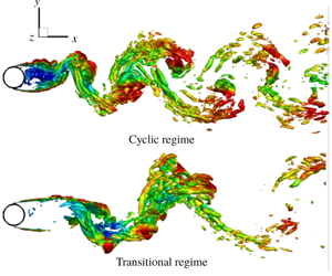
Cavitation refers to phase change of liquid into vapour as the liquid pressure drops below the vapour pressure. It is often encountered in hydrodynamic applications such as marine propulsors, hydrofoils and rotating turbomachinery. Cavitation can be a major source of noise, vibrations and material damage in such systems. Fry (Reference Fry1984) characterizes cavitation over a circular cylinder as belonging to cyclic and transitional regimes. As the cavitation number ($\unicode[STIX]{x1D70E}=(p_{\infty }-p_{v})/((1/2)\unicode[STIX]{x1D70C}_{\infty }U_{\infty }^{2})$, where $p_{\infty }$, $\unicode[STIX]{x1D70C}_{\infty }$ and $U_{\infty }$ are pressure, density and velocity in the free stream, respectively) in the free stream is sufficiently dropped, cavities develop inside the core of the vortices shed from either side of the cylinder, which is referred to as cyclic cavitation. With further reduction in $\unicode[STIX]{x1D70E}$, in the transitional regime, the cavities grow larger in size and begin to interact with each other, causing the cavity shedding to become irregular, until they coalesce to form a single cavity fixed to the cylinder. It is observed that noise and erosion rates peak at the transition from the cyclic to the transitional regime as the cavities begin to interact (Fry Reference Fry1984). In the present investigation, we study cavitation over a circular cylinder over a range of $\unicode[STIX]{x1D70E}$ spanning the non-cavitating, cyclic and transitional cavitation regimes. We observe that cavitation inside the Kármán vortices in the cyclic regime, is significantly altered at the onset of ‘condensation shock’ propagation in the transitional regime. At the transition, an order of magnitude jump in shedding Strouhal number, a peak in pressure fluctuations and a maximum in $St$ versus $\unicode[STIX]{x1D70E}$ based on a cavity length are observed. Hence, changes in shedding characteristics in these regimes and condensation shock propagation are studied. It is also known that, non-condensable gas (NCG) can change acoustic properties such as sound speed, acoustic impedance and consequently the shock propagation. This motivates the study of NCG effects on cavity shedding and condensation shock propagation.

It is known that the sound speed of the two-phase water–vapour mixture is orders of magnitude smaller than the speed of sound of its constituent phases (Franc & Michel Reference Franc and Michel2005). If the sound speed becomes comparable to the magnitude of the velocities in the flow, it can lead to the formation of shock waves. Observation of shock waves in bubbly mixtures have been made as early as 1964 in the head breakdown process in cavitating inducers (Jakobsen Reference Jakobsen1964), although, ‘condensation shock’ propagation as a mechanism for partial cavity shedding has been shown only recently (Ganesh, Makiharju & Ceccio Reference Ganesh, Makiharju and Ceccio2016). Note that ‘condensation shocks’ refer to shock waves associated with a retracting partial cavity, typically have a weak discontinuity in pressure (order of few kPa) and involve phase change (Budich, Schmidt & Adams Reference Budich, Schmidt and Adams2018). Subsequent to Ganesh et al. (Reference Ganesh, Makiharju and Ceccio2016), various computational and experimental studies have considered condensation shock propagation as a mechanism in context of sheet to cloud cavitation (Schenke & van Terwisga Reference Schenke and van Terwisga2017; Wu, Maheux & Chahine Reference Wu, Maheux and Chahine2017; Bhatt & Mahesh Reference Bhatt and Mahesh2018; Budich et al. Reference Budich, Schmidt and Adams2018; Jahangir, Hogendoorn & Poelma Reference Jahangir, Hogendoorn and Poelma2018). In these studies, at sufficiently small $\unicode[STIX]{x1D70E}$, the sheet to cloud transition is observed by the propagation of condensation shocks, instead of the classically observed re-entrant jet mechanism (Laberteaux & Ceccio Reference Laberteaux and Ceccio2001). Similarly, in the present work involving bluff body cavitation, with a significant reduction in $\unicode[STIX]{x1D70E}$ (moving from the cyclic to the transitional regime), we observe that the condensation shock propagation rather than a periodic cavitation inside Kármán vortices dominates the cavity shedding.

Presence of NCG can influence cavitating flows in various ways (Briancon-Marjollet, Franc & Michel Reference Briancon-Marjollet, Franc and Michel1990; Kawakami, Gin & Arndt Reference Kawakami, Gin and Arndt2005; Orley et al. Reference Orley, Trummler, Hickel, Mihatsch, Schmidt and Adams2015; Makiharju, Ganesh & Ceccio Reference Makiharju, Ganesh and Ceccio2017; Vennig et al. Reference Vennig, Smith, Brandner, Giosio and Pearce2017; Brandao, Bhatt & Mahesh Reference Brandao, Bhatt and Mahesh2018; Trummler et al. Reference Trummler, Freytag, Schmidt and Adams2018). Influence of dissolved and injected NCG in partial cavitation over a wedge has been considered by Makiharju et al. (Reference Makiharju, Ganesh and Ceccio2017). They found that injection of NCG into the cavity suppressed vapour formation, altering the dynamics of condensation shock formation. Vennig et al. (Reference Vennig, Smith, Brandner, Giosio and Pearce2017), in the experimental investigation on a flow over a hydrofoil, observed that for a flow rich in vapour/NCG nuclei, multiple shock waves are necessary for complete condensation and detachment of the cavity. Trummler et al. (Reference Trummler, Freytag, Schmidt and Adams2018) concluded that gas present in vapour bubbles would lead to stronger rebound and dampen the emitted shockwaves. A similar damping effect due to the presence of gas in the medium was also observed by Brandao et al. (Reference Brandao, Bhatt and Mahesh2018). In such flows it is also important to note the influence of the nuclei content of vapour/NCG. At a pressure lower than the vapour pressure, cavitation is triggered by imperfections in water, that are mostly small NCG or vapour bubbles (known as cavitation nuclei) that initiate the liquid breakdown (Franc & Michel Reference Franc and Michel2005). In addition, NCG can behave differently from vapour in response to pressure variations; gas can only experience volume change due to expansion/compression, while vapour can, in addition, undergo phase change due to evaporation/condensation. Since the NCG does not undergo phase change, the flow is more sensitive to the nuclei content of initially present NCG in the system than vapour. Numerical studies involving fully compressible formulation and a homogeneous mixture approach often use relatively high values of free-stream nuclei (Saito et al. Reference Saito, Takami, Nakamori and Ikohagi2007; Seo, Moon & Shin Reference Seo, Moon and Shin2008; Gnanaskandan & Mahesh Reference Gnanaskandan and Mahesh2016a,Reference Gnanaskandan and Maheshb; Bhatt & Mahesh Reference Bhatt and Mahesh2018), to avoid extremely small time steps due to the low Mach numbers in water. The studies have shown that good agreement with experiment is observed for large regions of vapour and developed cavitation regimes (Saito et al. Reference Saito, Takami, Nakamori and Ikohagi2007; Gnanaskandan & Mahesh Reference Gnanaskandan and Mahesh2016a; Bhatt & Mahesh Reference Bhatt and Mahesh2018). Cavitation inception and incipient cavitation are known to be highly sensitive to the nuclei size and their distribution (Hsiao & Chahine Reference Hsiao and Chahine2005). Hence, in the present work, we also consider the effect of free-stream nuclei of vapour/NCG on the cylinder wake.

Single-phase flow over circular cylinders has been studied extensively in the past. Limited studies exist on the cavitating flow over a cylinder (Rao & Chandrasekhara Reference Rao and Chandrasekhara1976; Ramamurthy & Bhaskaran Reference Ramamurthy and Bhaskaran1977; Fry Reference Fry1984; Seo et al. Reference Seo, Moon and Shin2008; Gnanaskandan & Mahesh Reference Gnanaskandan and Mahesh2016b; Kumar, Bakshi & Chatterjee Reference Kumar, Bakshi and Chatterjee2017a; Kumar, Chatterjee & Bakshi Reference Kumar, Chatterjee and Bakshi2017b). Fry (Reference Fry1984) investigated cavity dynamics in the cylinder wake by measuring noise spectra. The author observes a peak in pressure fluctuations as the cyclic cavitation inside the periodic vortex shedding transitions (with the reduction in $\unicode[STIX]{x1D70E}$) to irregular–regular vortex shedding, and eventually to a fixed cavity. Seo et al. (Reference Seo, Moon and Shin2008) studied cavitating flow at Reynolds number $(Re)=200$ and observed that the shock waves generated by the coherent collapse of the vapour cloud significantly change the aerodynamic noise characteristics. Kumar et al. (Reference Kumar, Chatterjee and Bakshi2017b) studied the cavitating structures of the near wake of a circular cylinder for a subcritical Reynolds number and concluded that the cavities originate primarily in the free shear layer, not in the wake or in the attached boundary layer. For the cyclic cavitation, Gnanaskandan & Mahesh (Reference Gnanaskandan and Mahesh2016b) explained the reduction in Kármán shedding frequency with the reduction in free-stream $\unicode[STIX]{x1D70E}$, using the increase in the vorticity dilatation term due to cavitation. At lower $\unicode[STIX]{x1D70E}$, they observe condensation front propagation for the transitional regime, but do not discuss the nature of the front or the alteration in shedding characteristics. Effects of NCG are not discussed in any of these works.

The objectives of this paper are to (i) investigate cavitating flow over a circular cylinder over a range of $\unicode[STIX]{x1D70E}$ spanning non-cavitating, cyclic and transitional cavitation regimes, (ii) discuss the changes in shedding characteristics over the regimes (e.g. significant drop in shedding frequency, condensation front propagation, peak in $St$ versus $\unicode[STIX]{x1D70E}$ and pressure fluctuations) using numerical results and dynamic mode decomposition, (iii) using the Rankine–Hugoniot jump conditions, discuss the condensation shock propagation in the transitional regime, (iv) extend the numerical method of Gnanaskandan & Mahesh (Reference Gnanaskandan and Mahesh2016b) based on a fully compressible formulation and a homogeneous mixture to include the NCG. Study the effect of NCG on the shedding characteristics, condensation shock propagation and effect of the free-stream nuclei content, (v) study the turbulent cavitating flow at $Re=3900$ and compare it to the past work and laminar flow simulations at $Re=200$.

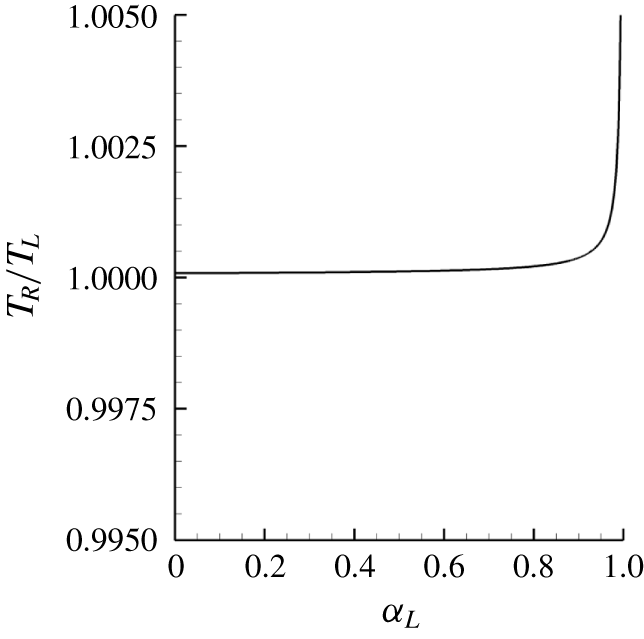
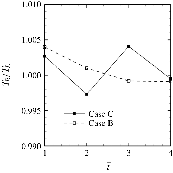
The paper is organized as follows. Section 2 discusses the physical model, the governing equations and the extension of the numerical method to account for NCG. The problem set-up and the simulation details are given in § 3. Results and discussions are provided in § 4. The paper is summarized in § 5. The appendix is devoted to the derivation of an equation for the speed of an upstream moving front using Rankine–Hugoniot jump conditions and a discussion about the temperature ratio across the condensation shock.

2 Physical model and numerical method

Numerical methods which include the effects of NCG were often based on the incompressible Navier–Stokes equations (Kunz et al. Reference Kunz, Boger, Stinebring, Chyczewski, Lindau, Gibeling, Venkateswaran and Govindan2000; Singhal et al. Reference Singhal, Athavale, Li and Jiang2002; Ji et al. Reference Ji, Luo, Peng, Zhang, Wu and Xu2010; Lu, Bark & Bensow Reference Lu, Bark and Bensow2012). More recently, fully compressible formulations have been employed (Orley et al. Reference Orley, Trummler, Hickel, Mihatsch, Schmidt and Adams2015; Mithun, Koukouvinis & Gavaises Reference Mithun, Koukouvinis and Gavaises2018). In the present work, the numerical method of Gnanaskandan & Mahesh (Reference Gnanaskandan and Mahesh2015), based on a fully compressible formulation for the vapour–water mixture, is extended to account for NCG. The ideal gas equation of state is used for NCG and is coupled with the stiffened equation of state for water and the ideal gas equation for vapour, to derive the mixture equation of state. The mixture sound speed is obtained from the mixture equation of state and the Gibbs equation. Transport equations for the non-condensable gas and the vapour mass fraction are solved along with the compressible Navier–Stokes equations for the mixture quantities. Both vapour and NCG are uniformly introduced in the free stream in terms of volume fraction. However, separate transport equations for vapour and gas allow both to evolve in a different manner, depending upon the local flow conditions, which allows study of their distribution in the wake of the cylinder.

2.1 Homogeneous mixture approach

We use the homogeneous mixture approach, where the mixture of water, vapour and NCG is considered as a single compressible medium. We assume mechanical equilibrium (i.e. each phase has the same pressure as the pressure of the cell and the slip velocity between the phases is not considered) and thermal equilibrium (i.e. temperature of each phase is same as the cell temperature). Surface tension effects are assumed small and hence neglected. The governing equations are the compressible Navier–Stokes equations for the mixture quantities along with transport equations for vapour and NCG. Different from the works of Orley et al. (Reference Orley, Trummler, Hickel, Mihatsch, Schmidt and Adams2015) and Mithun et al. (Reference Mithun, Koukouvinis and Gavaises2018), where the homogeneous equilibrium barotropic model is employed, here, we assume a finite mass transfer rate between vapour and water, which is explicitly modelled through source terms. These equations are Favre averaged and spatially filtered to perform large-eddy simulation (LES). The subgrid terms are modelled with the dynamic Smagorinsky model. Details can be found in Gnanaskandan & Mahesh (Reference Gnanaskandan and Mahesh2015). The unfiltered governing equations are

(2.1)

$$\begin{eqnarray}\left.\begin{array}{@{}c@{}}\displaystyle \frac{\unicode[STIX]{x2202}\unicode[STIX]{x1D70C}}{\unicode[STIX]{x2202}t}=-\frac{\unicode[STIX]{x2202}}{\unicode[STIX]{x2202}x_{j}}(\unicode[STIX]{x1D70C}u_{j}),\\ \displaystyle \frac{\unicode[STIX]{x2202}\unicode[STIX]{x1D70C}u_{i}}{\unicode[STIX]{x2202}t}=-\frac{\unicode[STIX]{x2202}}{\unicode[STIX]{x2202}x_{j}}(\unicode[STIX]{x1D70C}u_{i}u_{j}+p\unicode[STIX]{x1D6FF}_{ij}-\unicode[STIX]{x1D70E}_{ij}),\\ \displaystyle \frac{\unicode[STIX]{x2202}\unicode[STIX]{x1D70C}e_{s}}{\unicode[STIX]{x2202}t}=-\frac{\unicode[STIX]{x2202}}{\unicode[STIX]{x2202}x_{j}}(\unicode[STIX]{x1D70C}e_{s}u_{j}-Q_{j})-p\frac{\unicode[STIX]{x2202}u_{j}}{\unicode[STIX]{x2202}x_{j}}+\unicode[STIX]{x1D70E}_{ij}\frac{\unicode[STIX]{x2202}u_{i}}{\unicode[STIX]{x2202}x_{j}},\\ \displaystyle \frac{\unicode[STIX]{x2202}\unicode[STIX]{x1D70C}Y_{v}}{\unicode[STIX]{x2202}t}=-\frac{\unicode[STIX]{x2202}}{\unicode[STIX]{x2202}x_{j}}(\unicode[STIX]{x1D70C}Y_{v}u_{j})+S_{e}-S_{c}\quad \text{and}\\ \displaystyle \frac{\unicode[STIX]{x2202}\unicode[STIX]{x1D70C}Y_{g}}{\unicode[STIX]{x2202}t}=-\frac{\unicode[STIX]{x2202}}{\unicode[STIX]{x2202}x_{j}}(\unicode[STIX]{x1D70C}Y_{g}u_{j}).\end{array}\right\}\end{eqnarray}$$

Here $\unicode[STIX]{x1D70C}$, $u_{i}$, $e_{s}$ and $p$ are density, velocity, internal energy and pressure of the mixture respectively; $Y_{v}$ is the vapour mass fraction and $Y_{g}$ is the NCG mass fraction. The mixture density is defined as

(2.2)

$$\begin{eqnarray}\unicode[STIX]{x1D70C}=\unicode[STIX]{x1D70C}_{l}(1-\unicode[STIX]{x1D6FC}_{v}-\unicode[STIX]{x1D6FC}_{g})+\unicode[STIX]{x1D70C}_{v}\unicode[STIX]{x1D6FC}_{v}+\unicode[STIX]{x1D70C}_{g}\unicode[STIX]{x1D6FC}_{g},\end{eqnarray}$$

where $\unicode[STIX]{x1D70C}_{l}$, $\unicode[STIX]{x1D70C}_{v}$ and $\unicode[STIX]{x1D70C}_{g}$ are the densities of liquid, vapour and gas respectively; $\unicode[STIX]{x1D6FC}_{v}$ and $\unicode[STIX]{x1D6FC}_{g}$ are the volume fractions of vapour and NCG respectively. Volume fractions of each constituent phase are related to their respective mass fractions as

(2.3a-c)

$$\begin{eqnarray}\unicode[STIX]{x1D70C}_{l}(1-\unicode[STIX]{x1D6FC}_{v}-\unicode[STIX]{x1D6FC}_{g})=\unicode[STIX]{x1D70C}(1-Y_{v}-Y_{g}),\quad \unicode[STIX]{x1D70C}_{v}\unicode[STIX]{x1D6FC}_{v}=\unicode[STIX]{x1D70C}Y_{v}\quad \text{and}\quad \unicode[STIX]{x1D70C}_{g}\unicode[STIX]{x1D6FC}_{g}=\unicode[STIX]{x1D70C}Y_{g}.\end{eqnarray}$$

Internal energy of the mixture is obtained by a mass weighted average of its constituent phases

(2.4)

$$\begin{eqnarray}\left.\begin{array}{@{}c@{}}\displaystyle \unicode[STIX]{x1D70C}e_{s}=\unicode[STIX]{x1D70C}(1-Y_{v}-Y_{g})e_{l}+\unicode[STIX]{x1D70C}Y_{v}e_{v}+\unicode[STIX]{x1D70C}Y_{g}e_{g},\quad \text{where}\\ \displaystyle e_{l}=C_{vl}T+\frac{P_{c}}{\unicode[STIX]{x1D70C}_{l}},\\ \displaystyle e_{v}=C_{vv}T\quad \text{and}\\ \displaystyle e_{g}=C_{vg}T.\end{array}\right\}\end{eqnarray}$$

Here, $e_{l}$, $e_{v}$ and $e_{g}$ are the internal energies of liquid, vapour and NCG respectively and $C_{vl}$, $C_{vv}$ and $C_{vg}$ are their specific heats at constant volume respectively; $T$ is the mixture temperature. The system is closed using a mixture equation of state obtained using a stiffened equation of state for the liquid and the ideal gas equation of state for both vapour and NCG,

(2.5)

$$\begin{eqnarray}p=Y_{v}\unicode[STIX]{x1D70C}R_{v}T+Y_{g}\unicode[STIX]{x1D70C}R_{g}T+(1-Y_{v}-Y_{g})\unicode[STIX]{x1D70C}K_{l}T\frac{p}{p+P_{c}},\end{eqnarray}$$

where $R_{v}=461.6~\text{J}~\text{kg}^{-1}~\text{K}^{-1}$, $R_{g}=286.9~\text{J}~\text{kg}^{-1}~\text{K}^{-1}$, $K_{l}=2684.075~\text{J}~\text{kg}^{-1}~\text{K}^{-1}$ and $P_{c}=786.333\times 10^{6}~\text{Pa}$ are the constants associated with the equation of state of the mixture. Parameters for the stiffened equation of state used for water are derived by Gnanaskandan & Mahesh (Reference Gnanaskandan and Mahesh2015) to match the speed of sound in liquid at a given density. Parameters for the gas and vapour equations of state are taken from White (Reference White2006) and Saito et al. (Reference Saito, Takami, Nakamori and Ikohagi2007) respectively. Hence, the current approach accurately predicts the liquid speed of sound and density variation as shown in Gnanaskandan & Mahesh (Reference Gnanaskandan and Mahesh2015), although the specific heat at constant volume is under predicted ($1500~\text{J}~\text{kg}^{-1}~\text{K}^{-1}$ as compared to the National Institute of Standards and Technology (NIST) value of $4157.4~\text{J}~\text{kg}^{-1}~\text{K}^{-1}$). This however, is not considered as a serious drawback, considering the isothermal nature of the current problem, as discussed in appendix B. In addition, numerical studies of Gnanaskandan & Mahesh (Reference Gnanaskandan and Mahesh2015) have demonstrated validation of the numerical method using a stiffened equation of state for a variety of flow problems for the study of hydrodynamic cavitation.

The viscous stress tensor ($\unicode[STIX]{x1D748}$) and heat flux vector ($\boldsymbol{Q}$) are given by

(2.6a,b)

$$\begin{eqnarray}\unicode[STIX]{x1D70E}_{ij}=\unicode[STIX]{x1D707}\left(\frac{\unicode[STIX]{x2202}u_{i}}{\unicode[STIX]{x2202}x_{j}}+\frac{\unicode[STIX]{x2202}u_{j}}{\unicode[STIX]{x2202}u_{i}}-\frac{2}{3}\frac{\unicode[STIX]{x2202}u_{k}}{\unicode[STIX]{x2202}x_{k}}\unicode[STIX]{x1D6FF}_{ij}\right)\quad \text{and}\quad Q_{j}=k\frac{\unicode[STIX]{x2202}T}{\unicode[STIX]{x2202}x_{j}},\end{eqnarray}$$

where the mixture thermal conductivity is defined as a volume average between the conductivities of the individual constituent phases. For the mixture viscosity, we follow Beattie & Whalley (Reference Beattie and Whalley1982) and assume that the effective dynamic viscosity of the liquid–vapour–gas mixture satisfies a quadratic law with a maximum in the two-phase region. The mixture thermal conductivity and viscosity are given as

(2.7)

$$\begin{eqnarray}\left.\begin{array}{@{}c@{}}\displaystyle \unicode[STIX]{x1D707}=\unicode[STIX]{x1D707}_{l}(1-\unicode[STIX]{x1D6FC}_{v}-\unicode[STIX]{x1D6FC}_{g})(1+2.5(\unicode[STIX]{x1D6FC}_{v}+\unicode[STIX]{x1D6FC}_{g}))+\unicode[STIX]{x1D707}_{v}\unicode[STIX]{x1D6FC}_{v}+\unicode[STIX]{x1D707}_{g}\unicode[STIX]{x1D6FC}_{g}\quad \text{and}\\ \displaystyle k=k_{l}(1-\unicode[STIX]{x1D6FC}_{v}-\unicode[STIX]{x1D6FC}_{g})+k_{v}\unicode[STIX]{x1D6FC}_{v}+k_{g}\unicode[STIX]{x1D6FC}_{g}.\end{array}\right\}\end{eqnarray}$$

In (2.7), $k_{l}$, $k_{v}$, and $k_{g}$ are the thermal conductivities of water, vapour and NCG respectively while $\unicode[STIX]{x1D707}_{l}$, $\unicode[STIX]{x1D707}_{v}$ and $\unicode[STIX]{x1D707}_{g}$ are the dynamic viscosities of water, vapour and NCG respectively. Note that $\unicode[STIX]{x1D707}_{l}\gg \unicode[STIX]{x1D707}_{v}$, $\unicode[STIX]{x1D707}_{g}$. A simple volume average would give a maximum in the liquid region for $\unicode[STIX]{x1D6FC}_{v}+\unicode[STIX]{x1D6FC}_{g}=0$ (i.e. in the liquid), while a quadratic dependence in Beattie & Whalley (Reference Beattie and Whalley1982) yields an initial increase in the mixture viscosity, moving from liquid to the mixture. The mixture viscosity is maximum in the two-phase region near the liquid. Molecular dynamics simulations confirm this behaviour (Chen et al. Reference Chen, Xue, Mahesh and Siepmann2019). They are related to the temperature of the mixture as

(2.8a-c)

$$\begin{eqnarray}\unicode[STIX]{x1D707}_{l}=C_{0l}\times 10^{C_{1l}/(T-C_{2l})},\quad \unicode[STIX]{x1D707}_{v}=C_{0v}\left(\frac{T}{T_{0v}}\right)^{n_{v}},\quad \unicode[STIX]{x1D707}_{g}=C_{0g}\left(\frac{T}{T_{0g}}\right)^{n_{g}},\end{eqnarray}$$

where the constants in (2.8) and their references are given in table 1. Thermal conductivity in a constituent phase ($k_{l}$, $k_{v}$ and $k_{g}$ respectively in liquid, vapour and NCG) is obtained from the Prandtl number ($Pr$) in each phase. Since the maximum observed values of vapour mass fractions in the cases considered are orders of magnitude smaller than unity, latent heat of vaporization can be neglected (Gnanaskandan & Mahesh Reference Gnanaskandan and Mahesh2015) and it was not considered in the present work. The parameters $S_{e}$ and $S_{c}$ are the source terms due to evaporation of water and condensation of vapour and are given by

(2.9)

$$\begin{eqnarray}\left.\begin{array}{@{}c@{}}\displaystyle S_{e}=C_{e}(\unicode[STIX]{x1D6FC}_{v}+\unicode[STIX]{x1D6FC}_{g})^{2}(1-\unicode[STIX]{x1D6FC}_{v}-\unicode[STIX]{x1D6FC}_{g})^{2}\frac{\unicode[STIX]{x1D70C}_{l}}{\unicode[STIX]{x1D70C}_{v}}\frac{\max ((p_{v}-p),0)}{\sqrt{2\unicode[STIX]{x03C0}R_{v}T_{s}}}\quad \text{and}\\ \displaystyle S_{c}=C_{c}(\unicode[STIX]{x1D6FC}_{v}+\unicode[STIX]{x1D6FC}_{g})^{2}(1-\unicode[STIX]{x1D6FC}_{v}-\unicode[STIX]{x1D6FC}_{g})^{2}\frac{\max ((p-p_{v}),0)}{\sqrt{2\unicode[STIX]{x03C0}R_{v}T_{s}}}.\end{array}\right\}\end{eqnarray}$$

Here, $T_{s}$ is a reference temperature; $C_{e}$ and $C_{c}$ are empirical constants based on the interfacial area per unit volume and their values are taken to be equal to $0.1~\text{m}^{-1}$, as described by Saito et al. (Reference Saito, Takami, Nakamori and Ikohagi2007). They have shown that the solution is not sensitive to the value of empirical constants using cavitating flow over hemispherical/cylindrical bodies. The parameter $p_{v}$ is the vapour pressure, which is related to temperature as

(2.10)

$$\begin{eqnarray}p_{v}=p_{k}\exp \left(\left(1-\frac{T_{k}}{T}\right)(a+(b-cT)(T-d)^{2})\right),\end{eqnarray}$$

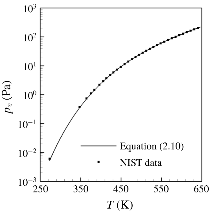
where $p_{k}=22.130~\text{MPa}$, $T_{k}=647.31~\text{K}$, $a=7.21$, $b=1.152\times 10^{-5}$, $c=-4.787\times 10^{-9}$ and $d=483.16$ (Saito et al. Reference Saito, Takami, Nakamori and Ikohagi2007). Vapour pressure variation with temperature obtained from (2.10) is compared to the NIST data in figure 1, showing excellent agreement.

Table 1.

Constants for species viscosity.

Figure 1.

Vapour pressure variation with temperature.

The expression for the speed of sound in the mixture is obtained from (2.5) and the Gibbs equation and is given by

(2.11)

$$\begin{eqnarray}\displaystyle \left.\begin{array}{@{}c@{}}\displaystyle a^{2}=\frac{C_{1}T}{C_{0}-C_{1}/C_{pm}},\quad \text{where}\\ \displaystyle C_{1}=(Y_{v}R_{v}+Y_{g}R_{g})(p+P_{c})+(1-Y_{v}-Y_{g})K_{l}p,\\ \displaystyle C_{0}=2p+P_{c}-\unicode[STIX]{x1D70C}T(Y_{v}R_{v}+Y_{g}R_{g})-(1-Y_{v}-Y_{g})\unicode[STIX]{x1D70C}K_{l}T\quad \text{and}\\ \displaystyle C_{pm}=Y_{g}C_{pg}+Y_{v}C_{pv}+(1-Y_{v}-Y_{g})C_{pl}.\end{array}\right\} & & \displaystyle\end{eqnarray}$$

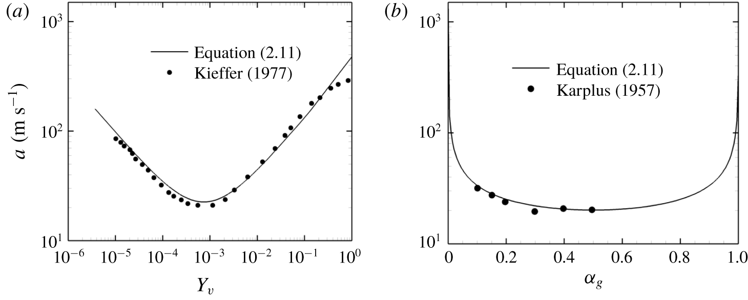
Here, $C_{pv}$, $C_{pg}$ and $C_{pl}$ are the specific heats at constant pressure for vapour, NCG and liquid respectively. Speed of sound obtained from (2.11) is compared to the experimentally available data for water–vapour mixtures of Kieffer (Reference Kieffer1977) as shown in figure 2(a) and water–air mixtures of Karplus (Reference Karplus1957) in figure 2(b). The speed of sound derived in the present work does not consider mass transfer effects, and hence is a frozen speed of sound.

Figure 2.

Speed of sound in water–vapour mixtures (a) and in water–NCG mixtures (b).

2.2 Numerical method

The numerical method of Gnanaskandan & Mahesh (Reference Gnanaskandan and Mahesh2015) is extended to include the effects of NCG. The algorithm has been extensively validated for water–vapour mixtures over a variety of problems by Gnanaskandan & Mahesh (Reference Gnanaskandan and Mahesh2015). The algorithm was used successfully to simulate both the re-entrant jet (Gnanaskandan & Mahesh Reference Gnanaskandan and Mahesh2016a) and condensation shock regimes (Bhatt & Mahesh Reference Bhatt and Mahesh2018) in sheet to cloud cavitation over a wedge. Thus we only focus on the details pertaining to the inclusion of NCG.

The algorithm uses a predictor–corrector approach. In the predictor step, the governing equations are spatially discretized using a symmetric non-dissipative finite volume scheme. The viscous fluxes are split into compressible and incompressible contributions and treated separately. Once the fluxes are obtained, a predicted value $\hat{\boldsymbol{q}}_{j}^{n+1}$ is computed using an explicit Adams–Bashforth time integration. The corrector step uses characteristic-based filtering to compute the final solution $\boldsymbol{q}_{j}^{n+1}$ from the predicted value $\hat{\boldsymbol{q}}_{j}^{n+1}$ as

(2.12)

$$\begin{eqnarray}\boldsymbol{q}_{j,cv}^{n+1}=\hat{\boldsymbol{q}_{j,cv}^{n+1}}-\frac{\unicode[STIX]{x0394}t}{V_{cv}}\mathop{\sum }_{faces}(\boldsymbol{F}_{f}^{\ast }n_{f})A_{f},\end{eqnarray}$$

where $F_{f}^{\ast }$ is the filter numerical flux of the following form:

(2.13)

$$\begin{eqnarray}\boldsymbol{F}_{f_{c}}^{\ast }={\textstyle \frac{1}{2}}R_{f_{c}}\unicode[STIX]{x1D731}_{\boldsymbol{f}\boldsymbol{c}}^{\ast }.\end{eqnarray}$$

Here, $R_{f_{c}}$ is the matrix of right eigenvectors at the face computed using the Roe average of the variables from left and right cell-centred values. The parameter $\unicode[STIX]{x1D731}_{\boldsymbol{f}\boldsymbol{c}}^{\ast }$ is a vector, the $l$th component of which, $\unicode[STIX]{x1D719}^{\ast l}$, is given by

(2.14)

$$\begin{eqnarray}\unicode[STIX]{x1D719}_{fc}^{\ast l}=k\unicode[STIX]{x1D703}_{fc}^{l}\unicode[STIX]{x1D719}_{fc}^{l},\end{eqnarray}$$

where $k$ is an adjustable parameter and $\unicode[STIX]{x1D703}_{fc}$ is Harten’s switch function, given by

(2.15a-c)

$$\begin{eqnarray}\unicode[STIX]{x1D703}_{fc}=\sqrt{0.5(\hat{\unicode[STIX]{x1D703}}_{icv1}^{2}+\hat{\unicode[STIX]{x1D703}}_{icv2}^{2})},\quad \hat{\unicode[STIX]{x1D703}}_{icv1}=\frac{|\unicode[STIX]{x1D6FD}_{fc}|-|\unicode[STIX]{x1D6FD}_{f1}|}{|\unicode[STIX]{x1D6FD}_{fc}|+|\unicode[STIX]{x1D6FD}_{f1}|},\quad \hat{\unicode[STIX]{x1D703}}_{icv2}=\frac{|\unicode[STIX]{x1D6FD}_{f2}|-|\unicode[STIX]{x1D6FD}_{fc}|}{|\unicode[STIX]{x1D6FD}_{f2}|+|\unicode[STIX]{x1D6FD}_{fc}|}.\end{eqnarray}$$

Here, $\unicode[STIX]{x1D6FD}_{f}=R_{f}^{-1}(\boldsymbol{q}_{icv2}-\boldsymbol{q}_{icv1})$ is the difference between characteristic variables across the face. For $\unicode[STIX]{x1D719}_{l}$, the Harten–Yee total variation diminishing (TVD) form is used, as suggested by Yee, Sandham & Djomehri (Reference Yee, Sandham and Djomehri1999),

(2.16)

$$\begin{eqnarray}\left.\begin{array}{@{}c@{}}\displaystyle \unicode[STIX]{x1D719}_{fc}^{l}={\textstyle \frac{1}{2}}\unicode[STIX]{x1D6F9}(a_{fc}^{l})(g_{icv1}^{l}+g_{icv2}^{l})-\unicode[STIX]{x1D6F9}(a_{fc}^{l}+\unicode[STIX]{x1D6FE}_{fc}^{l})\unicode[STIX]{x1D6FD}_{fc}^{l},\\ \displaystyle \unicode[STIX]{x1D6FE}_{fc}^{l}=\frac{1}{2}\frac{\unicode[STIX]{x1D6F9}(a_{fc}^{l})(g_{icv2}^{l}-g_{icv1}^{l})\unicode[STIX]{x1D6FD}_{fc}^{l}}{(\unicode[STIX]{x1D6FD}_{fc}^{l})^{2}+\unicode[STIX]{x1D716}},\end{array}\right\}\end{eqnarray}$$

where $\unicode[STIX]{x1D716}=10^{-7}$, $\unicode[STIX]{x1D6F9}(z)=\sqrt{\unicode[STIX]{x1D6FF}+z^{2}}$ ($\unicode[STIX]{x1D6FF}$ being $1/16$) is introduced for entropy fixing and $a_{fc}^{l}$ is an eigenvalue of the Jacobian matrix. The limiter function $g_{icv}$ is computed using the minmod limiter, as described by Park & Mahesh (Reference Park and Mahesh2007) on unstructured grids.

Park & Mahesh (Reference Park and Mahesh2007) proposed a modification to Harten’s switch $\unicode[STIX]{x1D703}_{fc}$ to accurately represent under-resolved turbulence for single-phase flows by multiplying $\unicode[STIX]{x1D703}_{fc}$ by $\unicode[STIX]{x1D703}_{fc}^{\ast }$ as

(2.17)

$$\begin{eqnarray}\left.\begin{array}{@{}c@{}}\displaystyle \unicode[STIX]{x1D703}_{fc}=\unicode[STIX]{x1D703}_{fc}\unicode[STIX]{x1D703}_{fc}^{\ast },\\ \displaystyle \unicode[STIX]{x1D703}_{fc}^{\ast }={\textstyle \frac{1}{2}}(\unicode[STIX]{x1D703}_{icv1}^{\ast }+\unicode[STIX]{x1D703}_{icv2}^{\ast }),\\ \displaystyle \unicode[STIX]{x1D703}_{icv1}^{\ast }=\frac{(\unicode[STIX]{x1D735}\boldsymbol{\cdot }\boldsymbol{u})_{icv1}^{2}}{(\unicode[STIX]{x1D735}\boldsymbol{\cdot }\boldsymbol{u})_{icv1}^{2}+\unicode[STIX]{x1D6FA}_{icv1}^{2}+\unicode[STIX]{x1D716}}.\end{array}\right\}\end{eqnarray}$$

Gnanaskandan & Mahesh (Reference Gnanaskandan and Mahesh2015) modified it for a multiphase mixture of water and vapour to avoid the non-monotonic behaviour in the regions of flow cavitation as the single-phase switch, equation (2.17), reaches extremely small values due to high vorticity. This is given by

(2.18)

$$\begin{eqnarray}\unicode[STIX]{x1D703}_{fc}^{\ast }={\textstyle \frac{1}{2}}(\unicode[STIX]{x1D703}_{icv1}^{\ast }+\unicode[STIX]{x1D703}_{icv2}^{\ast })+|(\unicode[STIX]{x1D6FC}_{v_{icv2}}-\unicode[STIX]{x1D6FC}_{v_{icv1}})|.\end{eqnarray}$$

2.3 Modifications to the multiphase switch

While the modification proposed by Gnanaskandan & Mahesh (Reference Gnanaskandan and Mahesh2015) works well for a water–vapour mixture, it still does not prevent the non-monotonic behaviour when NCG is present. We illustrate this by considering a cavitating inviscid vortex. We consider a square domain of size $10R\times 10R$. The flow is initialized with the following velocity field:

(2.19)

$$\begin{eqnarray}\left.\begin{array}{@{}c@{}}\displaystyle u=-\frac{C(y-y_{c})}{R^{2}}\exp \left(\frac{-r^{2}}{2}\right)\quad \text{and}\\ \displaystyle v=\frac{C(x-x_{c})}{R^{2}}\exp \left(\frac{-r^{2}}{2}\right),\end{array}\right\}\end{eqnarray}$$

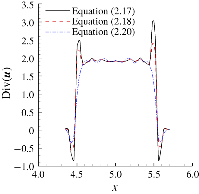
where $r=\sqrt{(x-x_{c})^{2}+(y-y_{c})^{2}}/R$, $R=1.0$, $C=5.0$ and $x_{c}=y_{c}=5R$. As we march in time, the pressure inside the vortex core drops, leading to flow cavitation and NCG expansion. We see non-monotonic behaviour in the solution, as illustrated by the flow velocity divergence in figure 3. As a remedy, an additional term due to the NCG volume fraction is added to the multiphase switch as

(2.20)

This additional term prevents non-monotonic behaviour due to the expansion of NCG in the low pressure regions, as shown in the figure 3. This term goes to zero in the absence of non-condensable gas. Hence, $\unicode[STIX]{x1D703}_{fc}$ as defined by (2.20) is used for the computation of $\unicode[STIX]{x1D703}_{fc}^{l}$ in (2.14).

Figure 3.

Line extracted along the vortex centreline showing absence of ‘non-monotonic behaviour’ with the modified switch.

3 Problem set-up

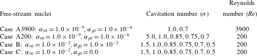
Table 2 lists the flow conditions considered for the simulations. The cavitation number in the free stream is $\unicode[STIX]{x1D70E}=(p_{\infty }-p_{v})/((1/2)\unicode[STIX]{x1D70C}_{\infty }U_{\infty })$, where $p_{\infty }$, $\unicode[STIX]{x1D70C}_{\infty }$ and $U_{\infty }$ are pressure, density and velocity in the free stream respectively. Cavitation number in the flow is varied from non-cavitating conditions to the cloud shedding regime. The Reynolds numbers, defined as $Re=(\unicode[STIX]{x1D70C}_{\infty }U_{\infty }D)/\unicode[STIX]{x1D707}$, where $D$ is the cylinder diameter, used here are $Re=200$ and $Re=3900$ as considered by Gnanaskandan & Mahesh (Reference Gnanaskandan and Mahesh2016b) for investigation of cavitation in the near wake of a cylinder for a water–vapour mixture. The simulations are initialized with a spatially uniform void fraction of vapour ($\unicode[STIX]{x1D6FC}_{v0}$) that nucleates the cavitation. NCG ($\unicode[STIX]{x1D6FC}_{g0}$) is introduced in the free stream, similar to the vapour nuclei in a spatially uniform manner. Different amounts of free-stream vapour and gas volume fraction are used in this study. Details are provided in table 2, with the corresponding $\unicode[STIX]{x1D70E}$ and $Re$.

Table 2.

Cases showing flow conditions chosen for the problem.

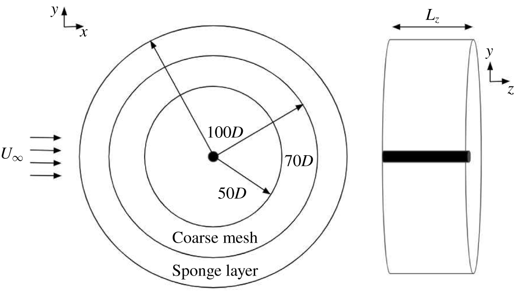
Figure 4 shows the schematic of the problem. The grid is two- and three-dimensional for the $Re=200$ and $Re=3900$ simulations, respectively. The domain size and mesh used in the present work are the same as the finer grid and larger domain size used by Gnanaskandan & Mahesh (Reference Gnanaskandan and Mahesh2016b). They performed a grid refinement study and showed that time evolution of lift/drag coefficient as well as the profiles of the mean and fluctuations in the void fraction show good agreement between their chosen grids. The computational domain is cylindrical with the origin at the centre of the cylinder. The domain is extended radially until $100D$ and covers a distance of $2\unicode[STIX]{x03C0}$ and $\unicode[STIX]{x03C0}$ in the spanwise direction for the two-dimensional and three-dimensional (2-D and 3-D) simulations respectively. The free-stream direction is in the positive $x$ direction as indicated by the arrows in figure 4. Free-stream conditions are imposed on all the far-field boundaries. Collapse of cavitation clouds produces strong pressure waves which propagate over the entire domain. In order to avoid reflection of these pressure waves from the boundaries, we apply acoustically absorbing sponge layers at the boundaries as shown in figure 4. This introduces an additional term in the governing equations (2.1) given by, $\unicode[STIX]{x1D6E4}(q-q_{ref})$. Here ‘$q$’ denotes the vector of conservative variables and the subscript ‘$ref$’ denotes the reference solution which the flow is damped to, which are free-stream values in the cases considered; ‘$\unicode[STIX]{x1D6E4}$’ denotes the amplitude of the forcing. In addition, the grid is coarsened in the far field to further reduce any reflections.

The mesh spacing considered near the cylinder surface is $0.005D\times 0.01D$ in the radial and azimuthal directions, which stretches to $0.03D\times 0.03D$ at approximately $2D$ downstream and then further stretches to $0.07D\times 0.07D$ at a distance of $5D$ downstream. For the 3-D grid required at $Re=3900$, 80 points are used in the spanwise direction while the same resolution as the 2-D grid is maintained in the $xy$ plane.

Figure 4.

Domain illustrating sponge layer and region of coarse mesh (not to scale).

Figure 5.

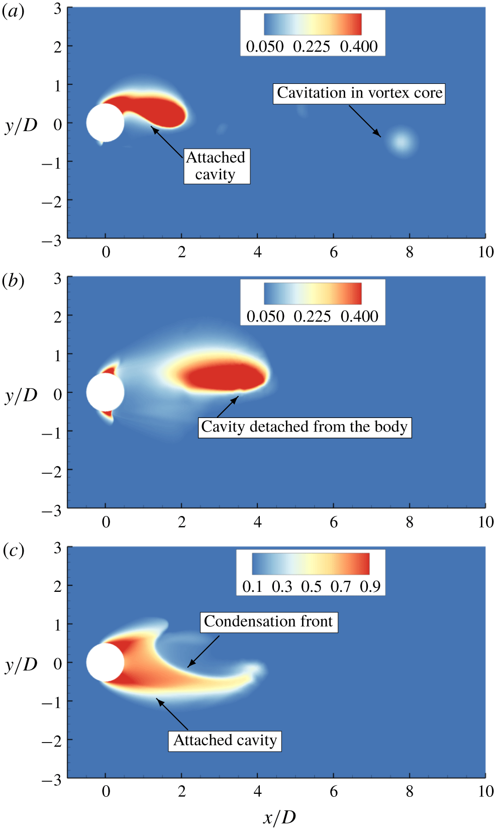
Instantaneous total void fraction (vapour $+$ NCG volume fraction) contour for the cyclic regime (a) and for the transitional regime (b,c) for case B. See supplementary movie 1 for the cyclic regime and supplementary movie 2 for the transitional regime, available at https://doi.org/10.1017/jfm.2019.971.

4 Results

Over the range of $\unicode[STIX]{x1D70E}$ studied, we observe two types of cavitation regime, as described by Fry (Reference Fry1984): cyclic and transitional. The cyclic cavitation regime is observed for high values of $\unicode[STIX]{x1D70E}$, and is characterized by periodic shedding of the cavitating vortices originating at the surface and is illustrated in figure 5(a). These cavitating vortices collapse as they move downstream into the region of high pressure, producing pressure waves. As $\unicode[STIX]{x1D70E}$ is reduced, the flow enters the transitional cavitation regime. Here, the cavity shedding process alternates between two phenomena. The first is similar to cyclic cavitation in the vortex cores; the difference however is that these vortex cores cavitate further downstream and the cavity thus formed is not attached to the cylinder. During this part of the cycle, the cylinder surface and immediate wake remain cavitation free, as shown in figure 5(b). This is followed by the second phenomenon where the instantaneous pressure in the immediate wake drops below vapour pressure, where a cavity forms symmetrically, spanning the entire aft body of the cylinder as shown in figure 5(c). Then, a pressure wave generated after the collapse of a vortex core impinges on the attached cavity, condensing it as displayed in figure 5(c). This is called a condensation front, or condensation shock if it moves at supersonic speed. Once this front hits the cylinder, it will lead to cavity detachment. Details of the shedding characteristics in these regimes are discussed in § 4.1. In § 4.2 we discuss the mean flow characteristics including vapour/NCG distribution in the cylinder wake and the boundary layer. Effects of free-stream void fraction on the boundary-layer separation and vapour/gas distribution are also discussed. In § 4.3 we show that the condensation fronts responsible for the cavity detachment travel at supersonic speed and that the condensation shocks are weakened by the NCG as they propagate towards the cylinder. Finally, large-eddy simulation of cavitating cylinder is presented and discussed in § 4.4.

4.1 Shedding characteristics

For single-phase flow over a bluff body, vortices shed periodically from the surface, forming the classical primary Kármán vortex street in the near wake. This is followed by a transition in the intermediate wake to a two-layered vortex street (e.g. Jiang & Cheng Reference Jiang and Cheng2019). The first vortex street transition was explained by Durgin & Karlsson (Reference Durgin and Karlsson1971) using a model in which the concentration of vorticity is strained into an elliptical shape by the nearby vortices in the street. This distorted vortex is then rotated, aligning its major axis with the streamwise direction. This process eventually results in distorted vortices merging and becoming shear layers on either side of the street. An important parameter that indicates the straining of the vortices and their merging is the spacing ratio, defined as the ratio between the cross-wake distance of differently signed vortices to the longitudinal distance between same sign vortices. In the experiments of Durgin & Karlsson (Reference Durgin and Karlsson1971), the authors found a spacing ratio greater than $0.366$ to be indicative of the transition, which was later confirmed by Karasudani & Funakoshi (Reference Karasudani and Funakoshi1994).

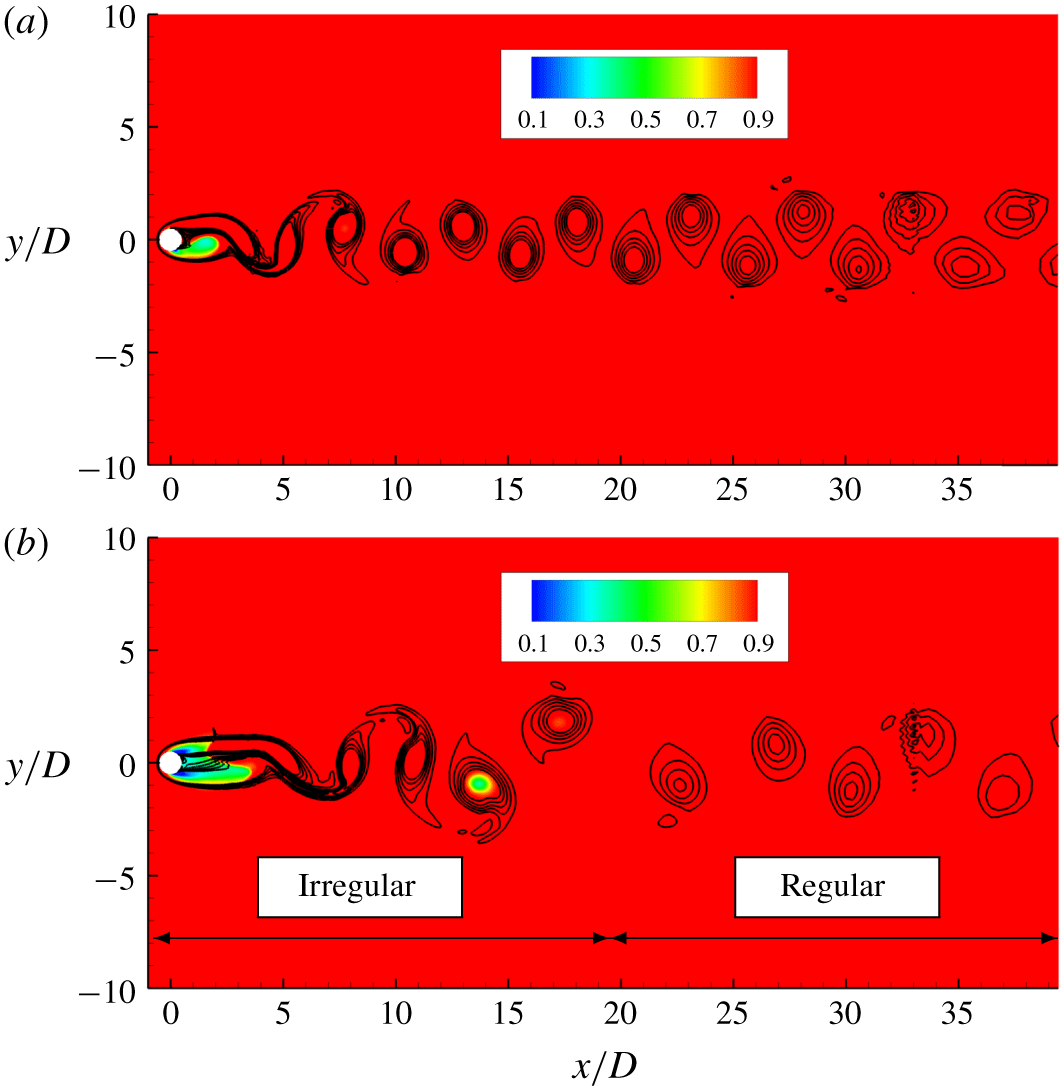
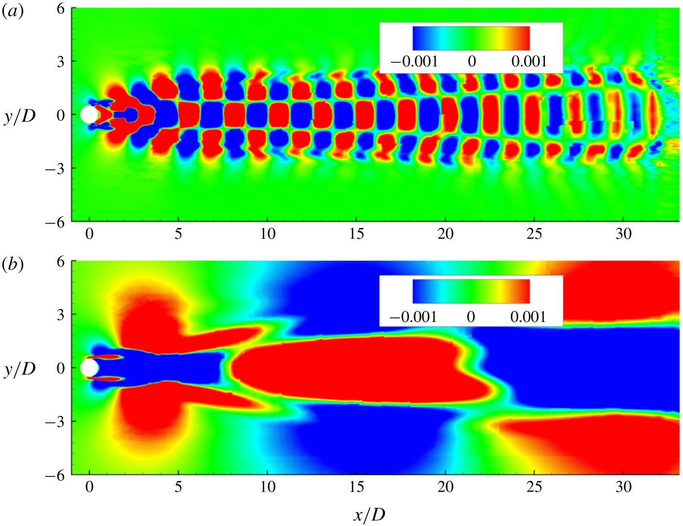
For cavitating flows, analysis of flow variables in the near wake can reveal both the vortex and/or cavity shedding frequency. In the cyclic regime (figure 6a), the dominant shedding frequency is that of a single cavitated vortex from the surface into the wake. Note the regular vortex shedding from top and bottom of the cylinder in this regime (figure 6a). In the transitional regime (figure 6b), we observe that this regular vortex shedding is disrupted at the onset of condensation front propagation, which occurs as the entire aft body of the cylinder cavitates due to lower $\unicode[STIX]{x1D70E}$. Consequently, the cylinder wake exhibits irregular and regular vortex shedding periodically (figure 6b). The dominant shedding frequency in the transitional regime indicates the cavity shedding after the passage of the condensation front and the recurrence of irregular and regular vortex shedding processes. The frequency of individual vortex shedding from the surface becomes secondary.

Figure 6.

Instantaneous solution indicating vortex shedding at $\unicode[STIX]{x1D70E}=1.0$ (a) and $\unicode[STIX]{x1D70E}=0.7$ (b) for case B. Lines indicate constant vorticity and coloured contours represent density.

4.1.1 $St$ versus $\unicode[STIX]{x1D70E}$

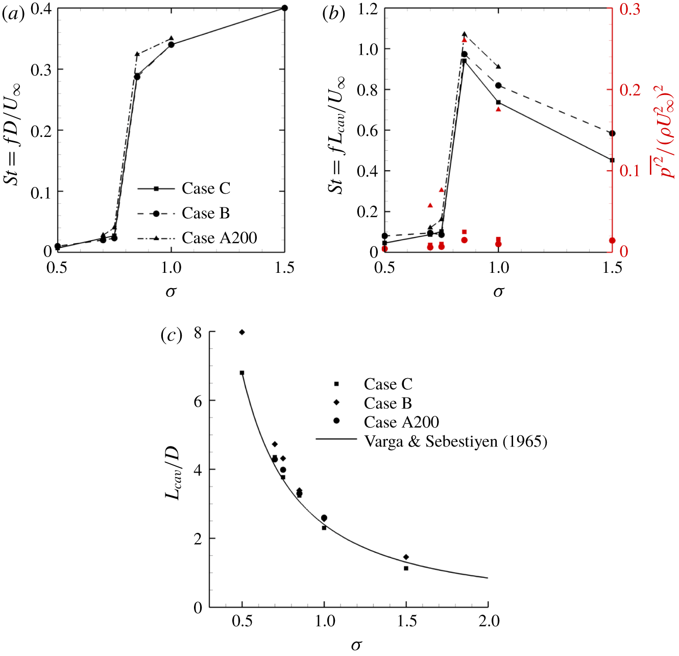
We define the Strouhal number ($St=fL/U$) to characterize the shedding frequency and plot it over a range of cavitation numbers spanning the cyclic and the transitional regimes, as shown in figure 7. Here, $f$ is the cavity shedding frequency obtained from the drag history, $U$ is the free-stream velocity and two length scales, $D$ and $L_{cav}$, are chosen for $L$ and plotted respectively in figures 7(a) and 7(b); $L_{cav}$ is the cavity length defined as the position along the wake centreline where the total void fraction decreases to a value lower than 0.05 (Ganesh et al. Reference Ganesh, Makiharju and Ceccio2016, Reference Ganesh, Deijlen, Bhatt, Wu and Ceccio2018). The values used to compute $St$ at different $\unicode[STIX]{x1D70E}$ in figure 7(b) are shown in figure 7(c) and compared to the experimental fit from Varga & Sebestiyen (Reference Varga and Sebestiyen1965) showing good agreement. We note that $St$ computed for non-cavitating conditions is 0.385. With reduction in $\unicode[STIX]{x1D70E}$, $St$ decreases in the cyclic regime. Gnanaskandan & Mahesh (Reference Gnanaskandan and Mahesh2016b) explained this behaviour through vorticity dilatation due to cavitation. However, the authors did not consider the sharp jump in $St$ moving through the transitional regime with further reduction in $\unicode[STIX]{x1D70E}$ (figure 7). Fry (Reference Fry1984) characterized the transition from the cyclic to the transitional regime by a peak in pressure fluctuations along the wake. Exactly at this transition, we observe that $St$ drops by an order of magnitude with $\unicode[STIX]{x1D70E}$ ($St=0.285$ at $\unicode[STIX]{x1D70E}=0.85$ to $St=0.018$ at $\unicode[STIX]{x1D70E}=0.75$) as the dominant frequency in the cyclic regime due to the periodic vortex shedding shifts to the frequency of irregular–regular vortex shedding in the transitional regime. In addition, a maximum in the $St$ versus $\unicode[STIX]{x1D70E}$ plot (figure 7b) is observed at $\unicode[STIX]{x1D70E}=0.85$ when $L_{cav}$ is chosen as a reference length. Young & Holl (Reference Young and Holl1966) and Ganesh et al. (Reference Ganesh, Deijlen, Bhatt, Wu and Ceccio2018) for flow over a triangular prism reported similar maximum in $St$ versus $\unicode[STIX]{x1D70E}$. They considered a configuration with flow confinement (top/bottom walls) and considered the base of the prism as the length scale.

Figure 7.

Value of $St$ for different $\unicode[STIX]{x1D70E}$ based on the cylinder diameter (a) and cavity length (b). Non-dimensional pressure fluctuations are represented by red symbols in (b) for case A200 (▲), case B (●) and case C (▪). Cavity length normalized by cylinder diameter for different $\unicode[STIX]{x1D70E}$ (c).

4.1.2 Effect of NCG

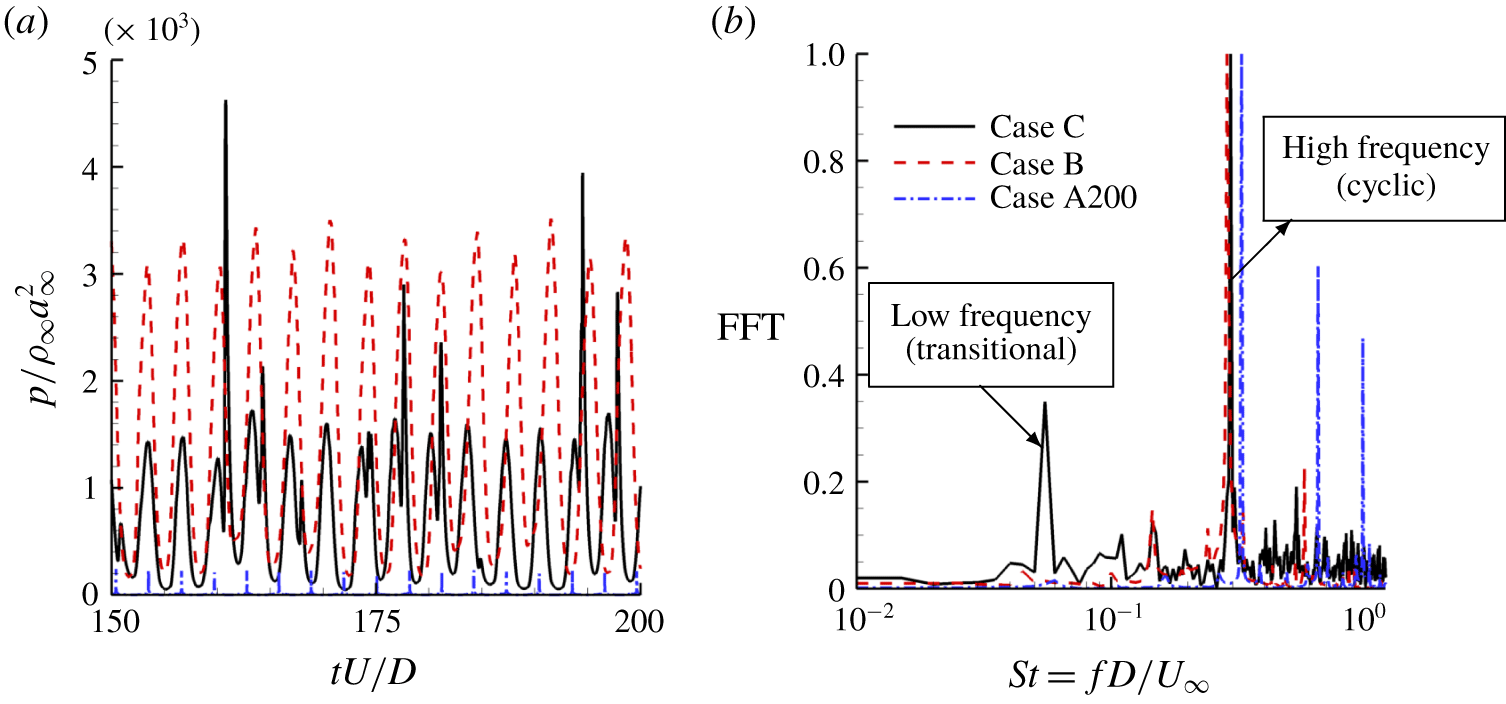
Note that $St$ corresponding to the dominant frequency of shedding plotted in figure 7 shows that the trend observed is not sensitive to the free-stream nuclei content of vapour and NCG. However, a small amount of NCG does influence the secondary shedding process, which is explained through the frequency components of the pressure history in the wake of the cylinder as shown in figure 8. We consider $\unicode[STIX]{x1D70E}=0.85$ corresponding to the cyclic cavitation regime near transition. The pressure history of flow without NCG exhibits both cyclic and transitional behaviour; the dominant frequency corresponds to cyclic shedding. In the presence of NCG, regardless of its free-stream nuclei content, the low frequency due to regular–irregular vortex shedding (figure 8b) of the transitional regime is completely suppressed. Thus, the presence of NCG can delay the transition from cyclic to transitional shedding.

Figure 8.

(a) Pressure signal at $x=2.5D$ in the cylinder wake scaled with free-stream density and speed of sound at $\unicode[STIX]{x1D70E}=0.85$ and (b) fast Fourier transform (FFT) of the corresponding signal scaled with its maximum value for better visualization.

4.1.3 Dynamic mode decomposition

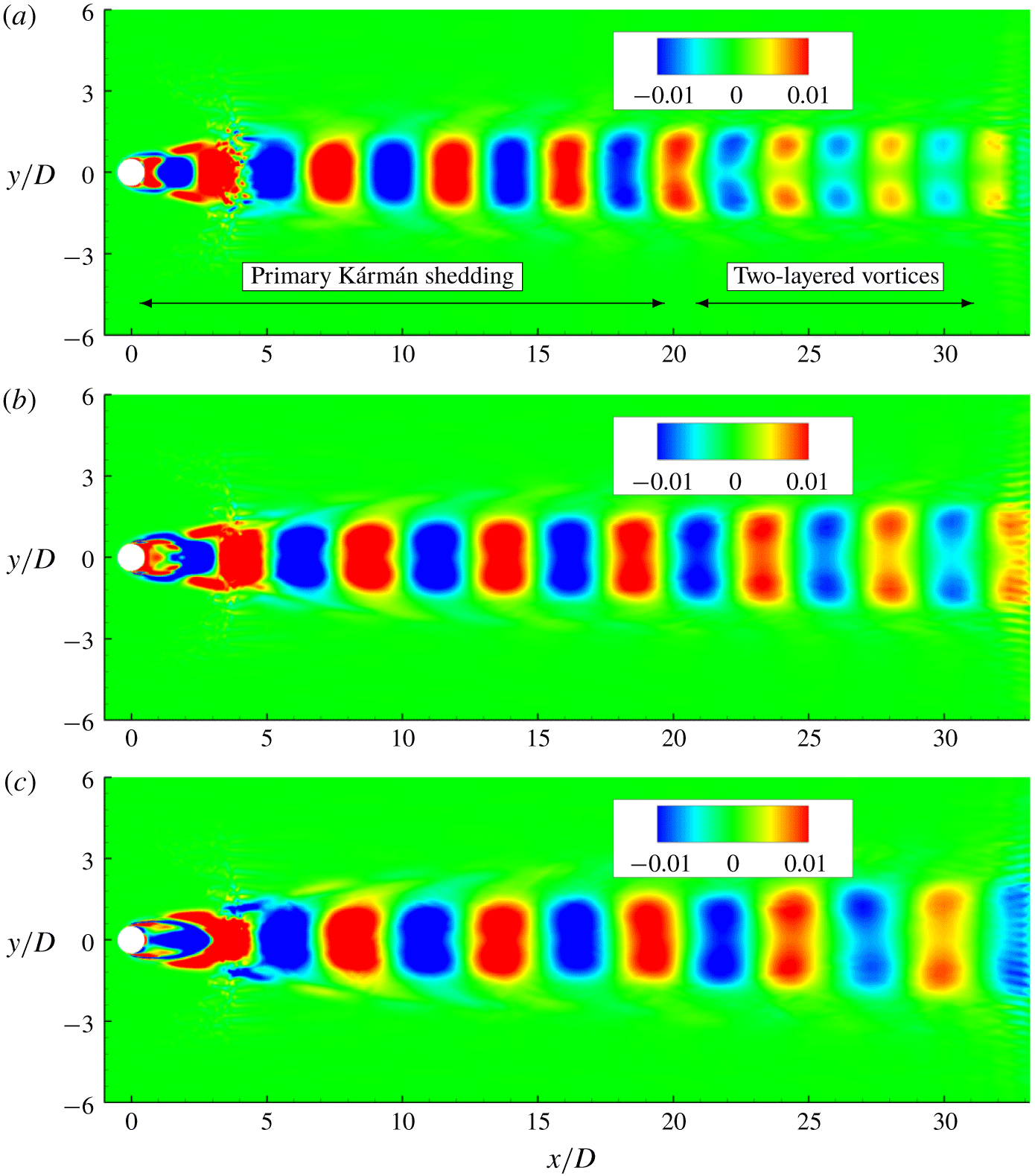
A detailed analysis of the behaviour behind the dominant frequencies in both the cyclic and the transitional, as well as in the non-cavitating regime, is considered by performing dynamic mode decomposition (DMD) and examining the corresponding modes. DMD is a data-driven modal decomposition technique that identifies a set of modes from multiple snapshots of the observable vectors. An eigenvalue is assigned to each of these modes, which denotes the growth/decay rate and oscillation frequency of the mode. The obtained modes and their eigenvalues capture the system dynamics. We use a novel DMD algorithm developed by Anantharamu & Mahesh (Reference Anantharamu and Mahesh2019) that has low computational cost and low memory requirements. The basic idea behind DMD is that the set of observable vectors (snapshot vectors of flow variables) $\{\unicode[STIX]{x1D713}_{i}\}_{i=1}^{N-1}$ can be written as a linear combination of DMD modes $\{\unicode[STIX]{x1D719}_{i}\}_{i=1}^{N-1}$ as

(4.1)

$$\begin{eqnarray}\unicode[STIX]{x1D713}_{i}=\mathop{\sum }_{j=1}^{N-1}c_{j}\unicode[STIX]{x1D706}_{j}\unicode[STIX]{x1D719}_{j};\quad i=1,\ldots ,N-1,\end{eqnarray}$$

where $\unicode[STIX]{x1D706}_{j}$ are the eigenvalues of the projected linear mapping and $c_{j}$ are the $j$th entries of the first vector $\unicode[STIX]{x1D713}_{1}$. The complete derivation of the algorithm can be seen in Anantharamu & Mahesh (Reference Anantharamu and Mahesh2019). For the cyclic and non-cavitating regime approximately $N=200$ snapshots of the flow field were taken with $\unicode[STIX]{x0394}t/(D/u_{\infty })=0.1$ between them, while $N=400$ snapshots with $\unicode[STIX]{x0394}t/(D/u_{\infty })=0.5$ were taken for the transitional regimes. We consider (i) the delay of Kármán vortex street transition to the two layer vortex street moving from non-cavitating to the cyclic cavitation regime and (ii) comparison of mode shapes in the cyclic and the transitional regimes.

The most dominant mode for case A200 at non-cavitating ($\unicode[STIX]{x1D70E}=5.0$) and cavitating conditions in the cyclic regime ($\unicode[STIX]{x1D70E}=1.0$ and $\unicode[STIX]{x1D70E}=0.85$), corresponds to the dominant frequencies in lift spectra and are shown in figure 9 coloured by spanwise vorticity. These dominant frequencies in the lift spectra indicate the shedding frequency of individual vortices. The dominant mode in figure 9(a) clearly reveals the primary Kármán vortex street and its transition to a two-layered vortex street. The streamwise position of this transition is $Re$ dependent and is observed at approximately $x=23D$ for the non-cavitating case in figure 9(a). Comparison to the cavitating cases in figures 9(b) and 9(c) reveals that this transition is delayed to $x=30D$ for $\unicode[STIX]{x1D70E}=1.0$ and to even farther distances at $\unicode[STIX]{x1D70E}=0.85$. This indicates that cavitation delays the first transition of the Kármán vortex street and that its distance from the cylinder grows with decreasing cavitation number.

Figure 9.

Most energetic modes coloured by spanwise vorticity at $\unicode[STIX]{x1D70E}=5.0$ (a), $\unicode[STIX]{x1D70E}=1.0$ (b) and $\unicode[STIX]{x1D70E}=0.85$ (c).

Figure 10.

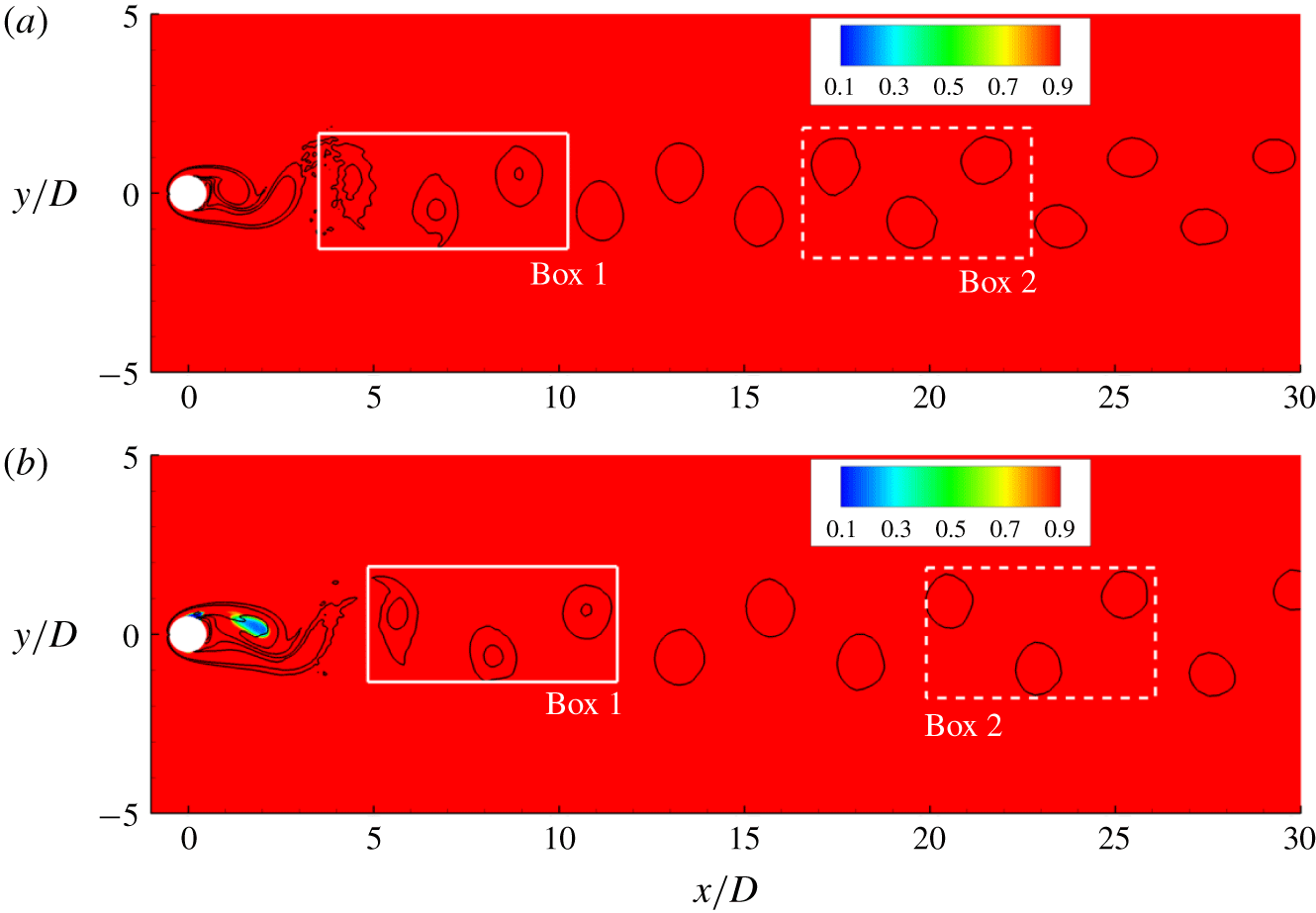
Vortex street coloured by density for $\unicode[STIX]{x1D70E}=5.0$ (a), $\unicode[STIX]{x1D70E}=1.0$ (b). White boxes indicate the region where the spacing ratio is computed.

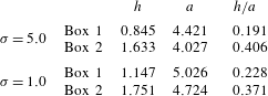
Figures 10(a) and 10(b) display the vortex street at $\unicode[STIX]{x1D70E}=5.0$ and $\unicode[STIX]{x1D70E}=1.0$ respectively. The vortices inside the boxes are used to compute the spacing ratio, as defined in § 4.1, at two streamwise positions: the first position is the closest possible to the cylinder and the second is just before the vortex street transition. Table 3 shows that for $\unicode[STIX]{x1D70E}=5.0$, the spacing ratio more than doubles over a small distance, quickly surpassing the $0.366$ threshold estimated by Durgin & Karlsson (Reference Durgin and Karlsson1971). Meanwhile, the spacing ratio for $\unicode[STIX]{x1D70E}=1.0$ grows slowly with streamwise distance and it is just slightly higher than the limit before the transition initiates. In order for the spacing ratio to be larger in the non-cavitating case, either the cross-wake distance $(h)$ has to be higher or the longitudinal distance $(a)$ has to be smaller. Table 3 reveals that it is the longitudinal distance between same sign vortices that is smaller for $\unicode[STIX]{x1D70E}=5.0$ at the two different streamwise positions. This parameter is inversely proportional to the shedding frequency of individual vortices, which is reduced from $0.193$ to $0.175$, based on lift history, when the cavitation number is lowered from $\unicode[STIX]{x1D70E}=5.0$ to $\unicode[STIX]{x1D70E}=1.0$. Thus, we can conclude that the reduction of shedding frequency due to cavitation plays a major role in delaying the first vortex street transition.

Table 3.

Cross-wake distance between different sign vortices $(h)$, longitudinal distance between same sign vortices $(a)$ and their ratio at two different wake positions for $\unicode[STIX]{x1D70E}=5.0$ and $\unicode[STIX]{x1D70E}=1.0$.

Mode shapes of axial velocity corresponding to the dominant frequency of the drag spectra are significantly altered moving from the cyclic to the transitional regime (figure 11). Length scales of the corresponding modes are an order of magnitude larger for the transitional regime, explaining the sharp jump in $St$. In the transitional regime (figure 11b), the modes are horizontally stretched and their length scales are significantly higher than the distance between subsequent vortex sheddings as observed in the cyclic regime (figure 11a). In addition, in the transitional regime immediately following the cylinder trailing edge, the mode shows a large region of negative axial velocity, suggesting the flow reversal due to the condensation front propagation.

Figure 11.

Modes corresponding to drag peak frequency at $\unicode[STIX]{x1D70E}=1.0$ (a) and $\unicode[STIX]{x1D70E}=0.7$ (b) for case A200, coloured with streamwise velocity.

4.2 Mean flow characteristics

4.2.1 Distribution of vapour and NCG in the cylinder wake

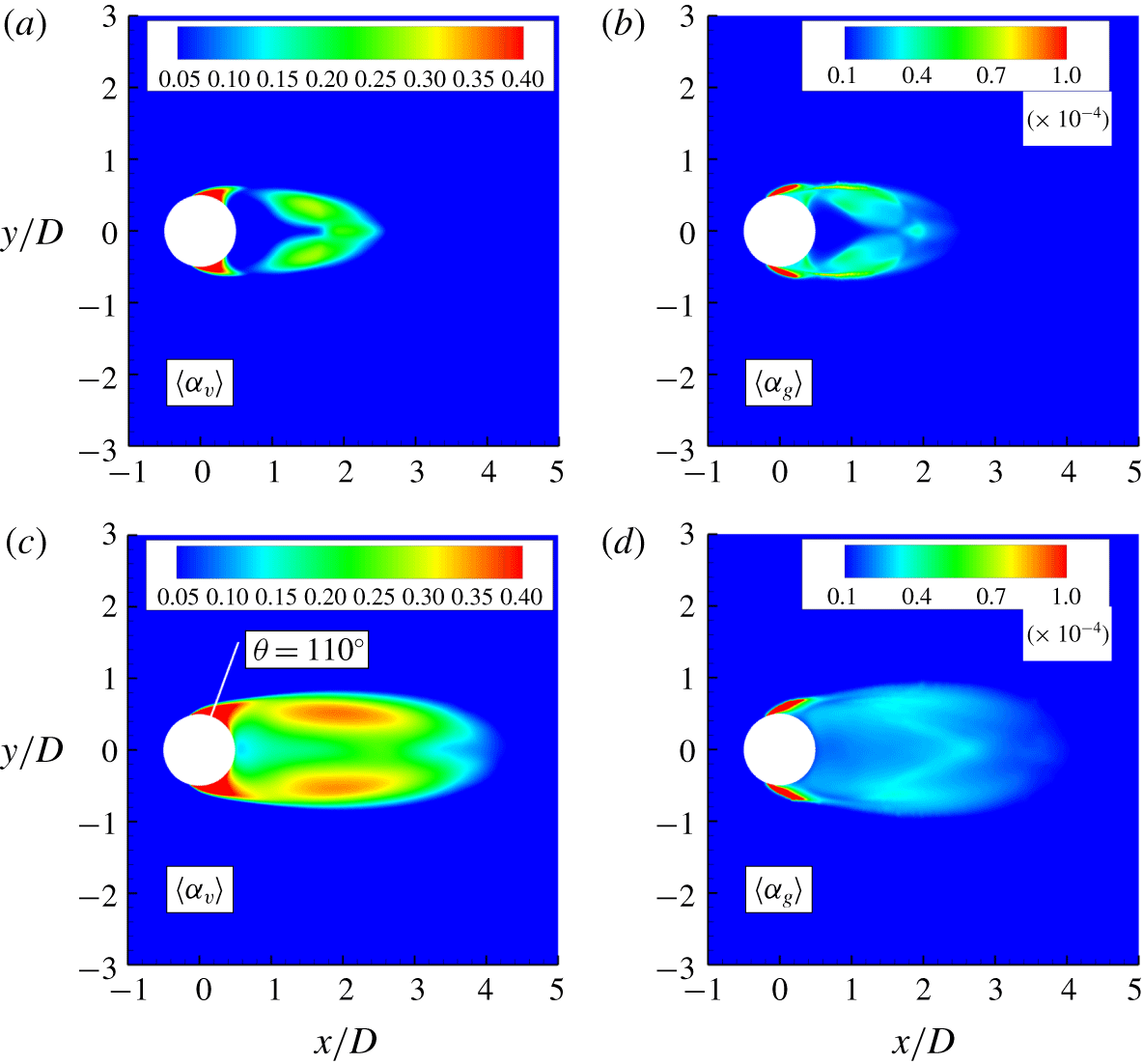
We consider the distribution of mean volume fraction of vapour and NCG in the near wake of the cylinder for case A200 at $\unicode[STIX]{x1D70E}=1$ and $0.7$, respectively in the cyclic and the transitional regimes, as shown in figure 12. In the cyclic regime (figure 12a,b), the majority of the vapour is concentrated on the cylinder surface and core of shed vortices from top and bottom. Regions near the cavity trailing edge and in the immediate wake remain cavitation free. NCG is concentrated in the incoming shear layer beginning at the cylinder surface into the near wake. Also, note that NCG is distributed in the neighbouring regions of the vapour concentration. NCG volume fractions are orders of magnitude smaller than vapour as additional NCG cannot be produced through phase change and volume fractions are observed only through expansion of the existing amount of gas in the free stream. In the transitional regime (figure 12c,d), in addition to the cylinder surface and the core of shed vortices, vapour is produced near the cavity trailing edge and in the immediate wake as the local pressure in the immediate wake drops below the vapour pressure with reduction in $\unicode[STIX]{x1D70E}$. NCG volume fractions are smaller than those observed in the cyclic regime and are concentrated mainly in the incoming shear layer.

Figure 12.

Time averaged vapour and NCG volume fraction contours respectively at $\unicode[STIX]{x1D70E}=1$ (a,b) and $\unicode[STIX]{x1D70E}=0.7$ (c,d) for the case A200. White line in (c) indicates azimuthal position of $110^{\circ }$.

4.2.2 Cavitation inside the boundary layer

In order to distinguish the mass transfer process due to phase change from expansion, we consider the local cavitation number which is defined as $\unicode[STIX]{x1D70E}_{loc}=(p_{loc}-p_{v})/(0.5\unicode[STIX]{x1D70C}_{\infty }u_{\infty }^{2})$, where $p_{loc}$ is the local pressure inside a cell. At a given instant if $\unicode[STIX]{x1D70E}_{loc}$ is positive in the region, the observed increase in vapour volume is only due to the expansion or the advection from nearby regions. If it is negative, the resulting increase in the volume of vapour is also accompanied by mass transfer. Consequently, in the regions of negative $\unicode[STIX]{x1D70E}_{loc}$, we expect the vapour to distinguish itself from NCG. 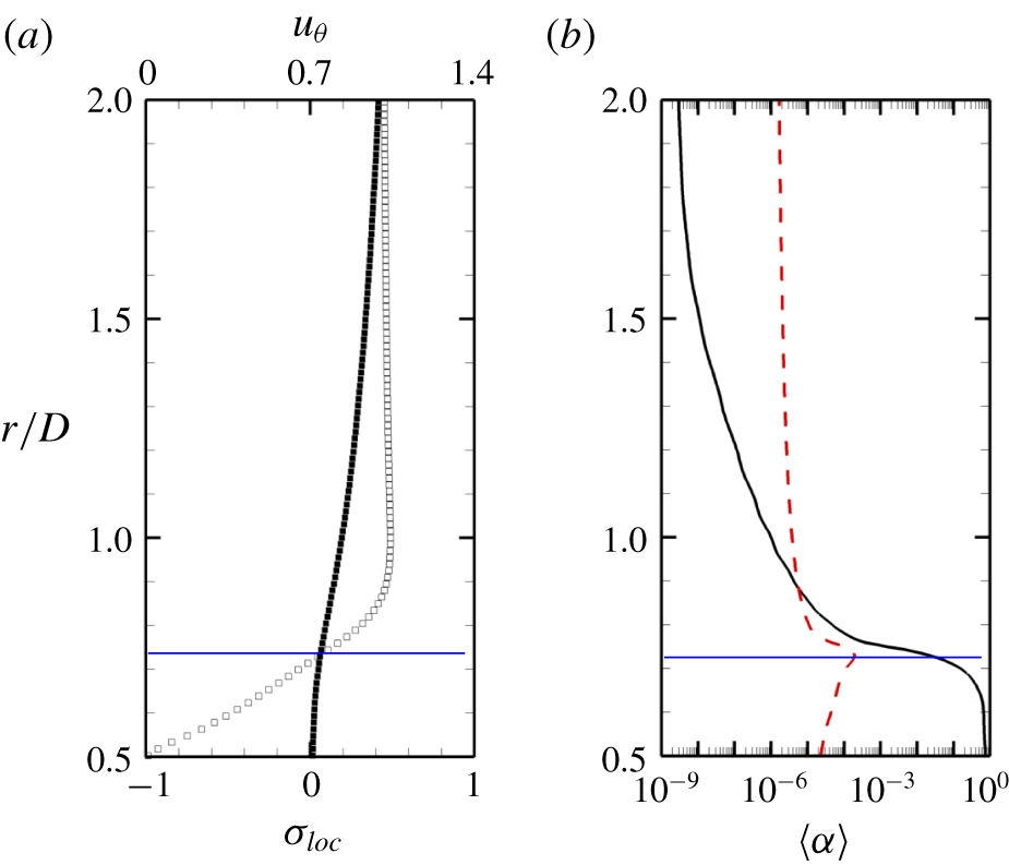We choose $\unicode[STIX]{x1D70E}=0.7$ and case A200 for explanation. Figure 13(a) shows the boundary-layer profile radially at $110^{\circ }$ from the leading edge (as indicated in figure 12c) of the cylinder along with $\unicode[STIX]{x1D70E}_{loc}$. The region separating positive $\unicode[STIX]{x1D70E}_{loc}$ within the boundary layer is indicated by the solid blue line. Note that vapour and NCG volume fractions deviate significantly in this region (figure 13b) as vapour is produced due to the mass transfer. The maximum NCG volume fraction is observed at $\unicode[STIX]{x1D70E}_{loc}=0$. As one moves radially outward, both vapour and NCG gas volume fractions are comparable in the remaining regions within the boundary layer, predominantly due to the expansion and the advection processes; finally reaching the corresponding free-stream values. Hence, cavitation as a mass transfer process is only observed in a finite near-wall region within the boundary layer.

Figure 13.

Cavitation inside the boundary layer at $\unicode[STIX]{x1D70E}=0.7$ and for case A200. Profiles taken at $110^{\circ }$ from the leading edge. (a) Azimuthal velocity profile (▫) with local cavitation number (▪) and (b) mean vapour (——) and NCG (– –) volume fractions.

4.2.3 Effect of free-stream nuclei

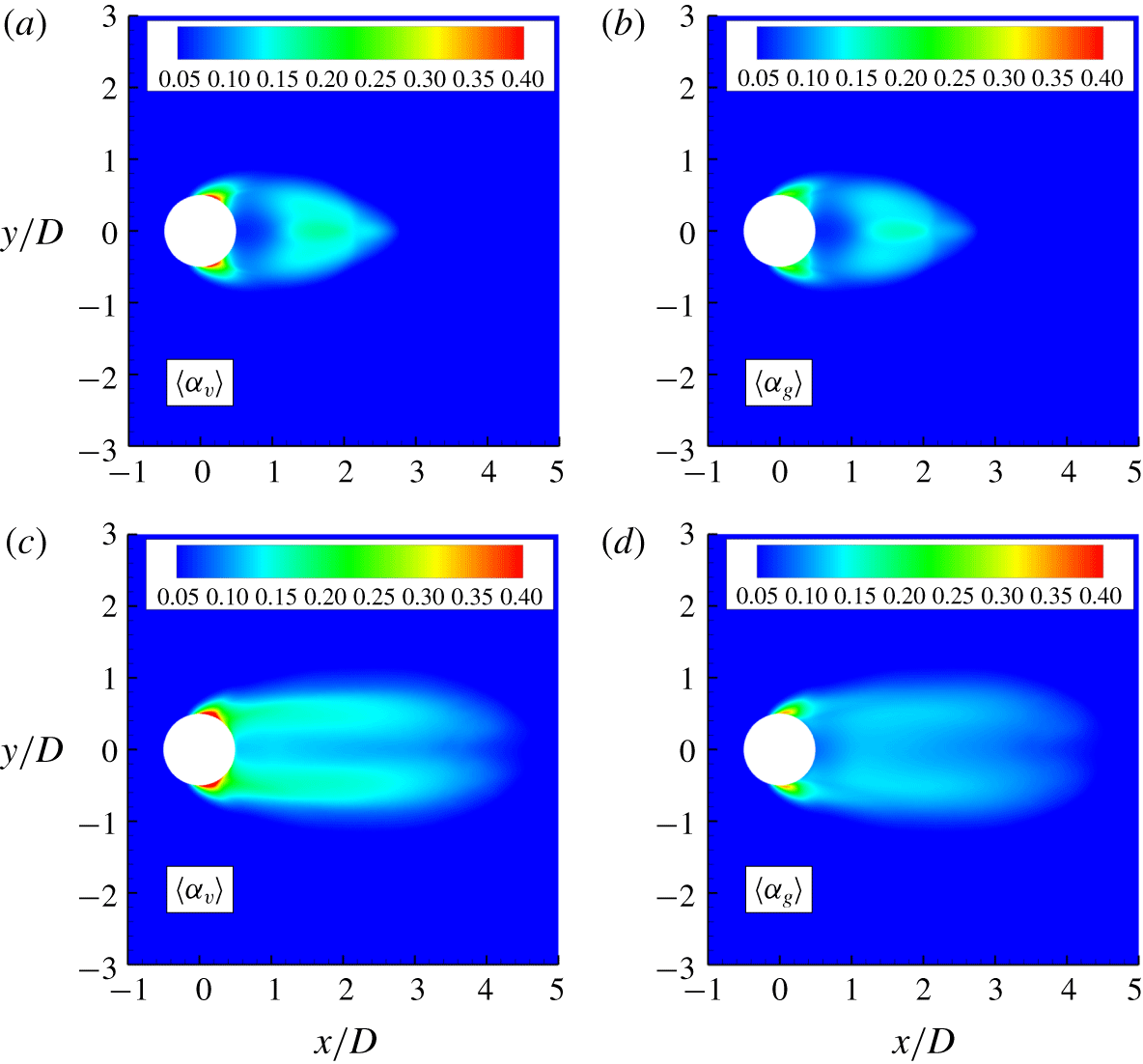
We discuss two important effects of the free-stream nuclei content: (i) distribution of vapour/NCG in the near wake and (ii) laminar separation of the boundary layer. Figure 14 shows the vapour/NCG distribution as discussed in § 4.2.1, although at a high concentration of vapour/NCG (case B). In the cyclic regime, vapour volume fractions show only minor differences in magnitude and distribution as compared to the low free-stream nuclei concentration (case A200, in figure 12). However, the NCG volume fraction is orders of magnitude higher as compared to the low free-stream nuclei case (figure 12b, figure 14b) and its distribution is almost indistinguishable from vapour at high nuclei concentration (figure 14a,b). As NCG does not undergo phase change, its initial concentration in the free stream has a very significant effect on the wake of the cylinder. While due to the significant effect of mass transfer, vapour is not as sensitive as NCG to the initial nuclei content. The same is also observed in the transitional regime (figure 14c,d). Note that vapour/gas diffusion can influence the distribution shown in the near wake. Although, we are unable to consider it at the current level of modelling.

Figure 14.

Time averaged vapour and NCG volume fraction contours respectively at $\unicode[STIX]{x1D70E}=1$ (a,b) and $\unicode[STIX]{x1D70E}=0.7$ (c,d) for case B.

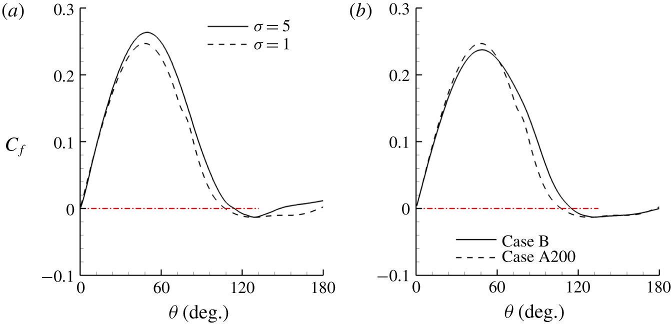
One point of divergence between experiments and simulations using the homogeneous mixture approach involves the location of boundary-layer separation. While experiments show that the boundary-layer separation point moves upstream along the cylinder as the flow cavitates (Arakeri Reference Arakeri1975), the same was not observed numerically by Gnanaskandan & Mahesh (Reference Gnanaskandan and Mahesh2016b). The reason behind this discrepancy, as explained in Gnanaskandan & Mahesh (Reference Gnanaskandan and Mahesh2016b), is the fact that the homogeneous mixture approach predicts the inception point upstream of the boundary-layer separation point. In our simulations with low free-stream void fraction (case A200), the inception point is also observed to be upstream of the separation point (not shown here). Differently from the work in Gnanaskandan & Mahesh (Reference Gnanaskandan and Mahesh2016b), where a high free-stream void fraction is employed, the boundary-layer separation point is shifted upstream as the cavitation number is reduced from a non-cavitating condition to a cavitating one when the free stream contains small amounts of vapour and gas (Case A200). This is evident from figure 15(a) that shows the skin friction along the cylinder surface, with the separation point shifting from $115^{\circ }$ to $106^{\circ }$ as $\unicode[STIX]{x1D70E}$ is reduced from 5.0 to 1.0.

It is found that the contents of vapour and NCG in the free stream have a significant impact on the separation point, as displayed in figure 15(b), with it moving downstream (from $106^{\circ }$ to $116^{\circ }$) as the free-stream volume fraction increases. In Gnanaskandan & Mahesh (Reference Gnanaskandan and Mahesh2016b), the authors discussed that the cavitation would start as soon as the local pressure is reduced to values below the vapour pressure. The expansion due to cavitation would then push the separation point downstream. The same behaviour is observable for case A200. Beside this is the fact that, before the flow cavitates, both vapour and gas travelling along the cylinder surface expand due to a decrease in pressure. Both the ideal gas expansion and the subsequently expansion due to phase change contribute to pushing the boundary-layer separation further downstream. The reason for case A200 showing the correct change in the boundary-layer separation point as the flow cavitates in comparison with the high volume fraction cases, however, lies on the fact that as the amounts of vapour and gas at the cylinder surface are substantially reduced, so are their effects on the flow due to ideal gas expansion. This leads to the conclusion that by adding NCG to a cavitating flow, the separation point would move downstream.

Figure 15.

Skin friction at different $\unicode[STIX]{x1D70E}$ for case A200 (a) and at $\unicode[STIX]{x1D70E}=1.0$ for different cases (b). The dash red line represents $C_{f}=0$ and indicates the separation point.

4.3 Condensation shock

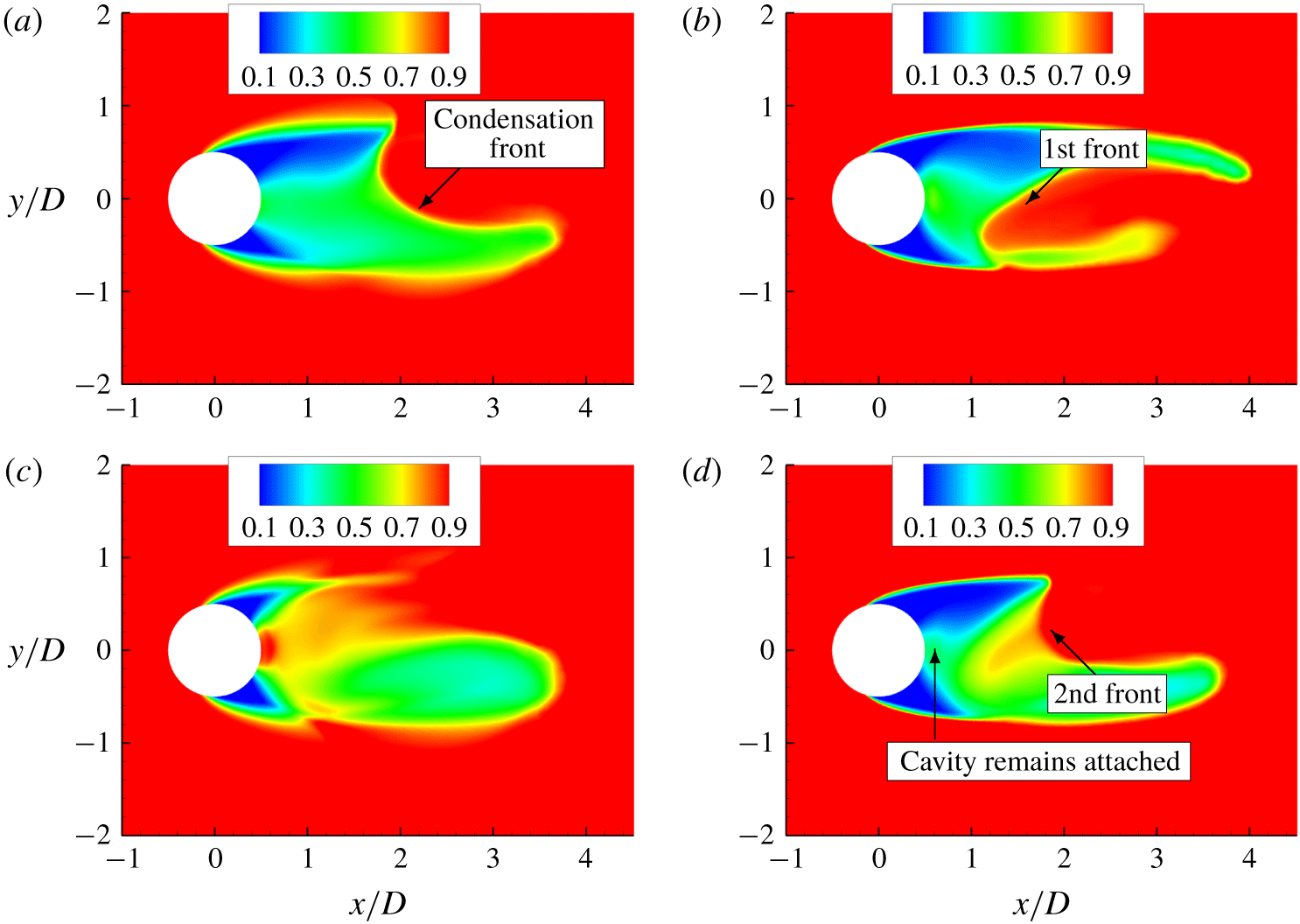
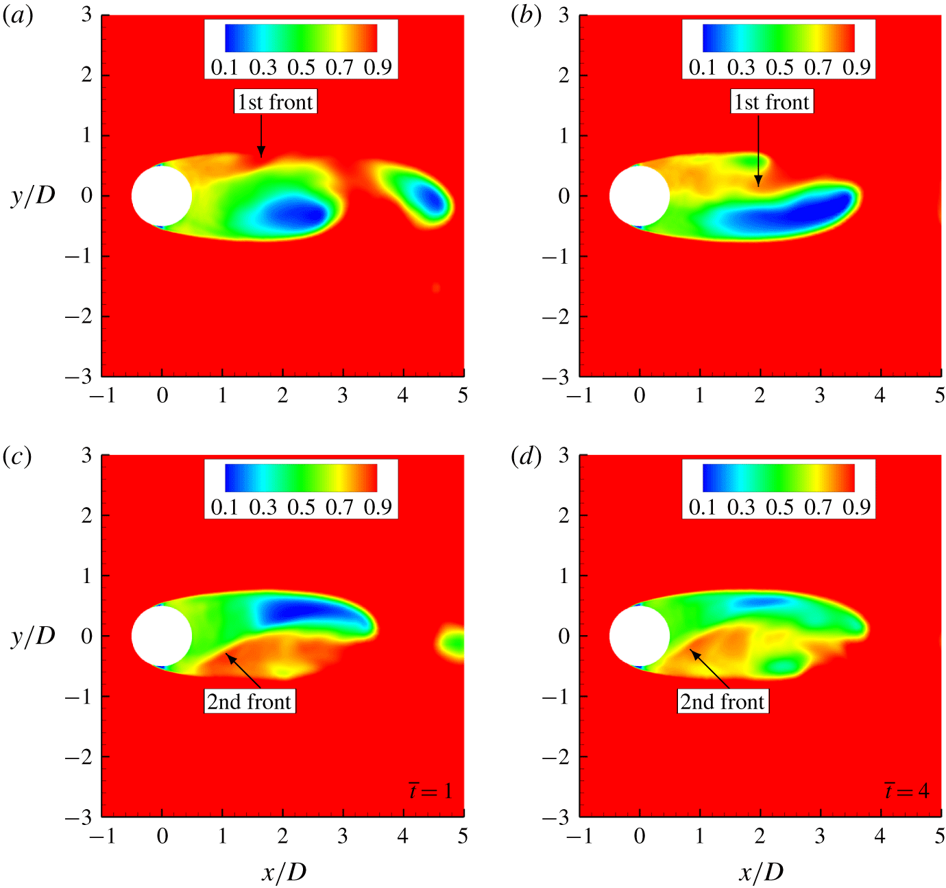
In this section, we consider the low frequency cavity shedding in the transitional regime using $\unicode[STIX]{x1D70E}=0.7$ to illustrate the shedding cycle in the presence (case A200) and absence (case C) of NCG. Figure 16 shows density contours taken at two different instances during the cycle for case C (figure 16a,c) and case A200 (figure 16b,d). The condensation front is visualized by the density discontinuity in the cavity closure region as indicated by the arrows in figure 16(a). As the front propagates upstream when NCG is absent, it condenses the vapour along the way, finally detaching the cavity completely as it impinges on the trailing edge of the cylinder, as shown in figure 16(c). In the presence of NCG however, figure 16(d) shows that the cavity remains attached after the cylinder is struck by the first propagating front. A second front is formed approaching the cylinder trailing edge. This indicates that when NCG is present, the pressure recovery in the back of the cylinder after the passage of the first front is not enough to condense the vapour and to compress large amounts of NCG in order to lead to cavity detachment. This indicates that a weaker condensation front impinges the cylinder surface in the presence of NCG. Likewise, Vennig et al. (Reference Vennig, Smith, Brandner, Giosio and Pearce2017), in the experimental investigation on a flow over a hydrofoil, observed that when the flow was rich in nuclei, a first shock wave only partially condensed the cavity prior to the passage of second shock wave leading to full spanwise detachment.

Figure 16.

Density contours showing the propagation of a condensation front in the absence (case C) (a,c) and presence (case A200) (b,d) of NCG.

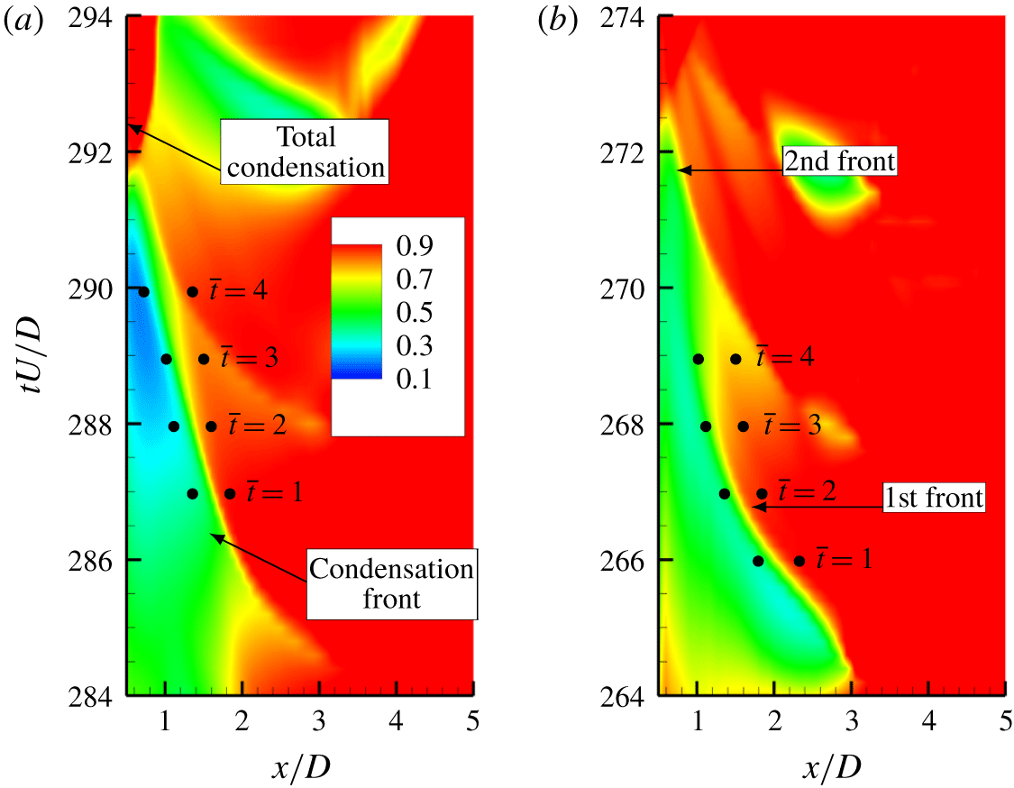
In order to quantify the behaviour we construct an $x-t$ diagram by taking data along the wake centreline (starting from trailing edge of the cylinder to a $5D$ distance along the wake) and stacking them in time. The $x-t$ diagram is shown in figures 17(a) and 17(b) for case C and case A200, respectively. The density discontinuity moving towards the cylinder when advancing in time indicates the condensation front. The slope of this discontinuity represents the inverse of the speed of the propagating front. It is evident here that in the presence of NCG, two fronts propagate before the complete detachment of the cavity as shown in figure 17(b). Curvature in the density discontinuity indicates that the speed of the condensation front changes as it travels towards the cylinder in the presence of NCG as compared to the almost straight line for the case without gas. Therefore, we use Rankine–Hugoniot jump conditions derived in appendix A at different time instances ($\overline{t}$), as given in figure 17, to obtain the speed of the front. Left and right states in (A 15) are obtained from quantities across the condensation front in the $x{-}t$ plot at the given time instants and are indicated by the bullet points. The speed of sound ahead of the front is obtained using (2.11).

Figure 17.

An $x{-}t$ plot of density along the wake centreline for $\unicode[STIX]{x1D70E}=0.7$ when (a) NCG is absent (case C) and (b) present (case A200).

4.3.1 Shock Mach numbers

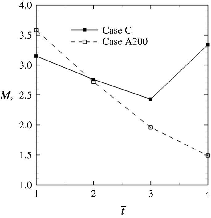
The speed of condensation front along with the sound speed allows us to comment on the Mach number at which the front propagates. Figure 18 shows the computed Mach number for the condensation front when NCG is absent (case C) and present (case A200) for the time instances mentioned in figure 17. Note that the computed Mach numbers refer to the first condensation front that impinges on the cylinder. Interestingly, all the Mach numbers in figure 18 are greater than 1, indicating that the front is indeed supersonic; it is henceforth referred to as condensation shock. An important distinction is that in the presence of NCG, the Mach number at which the condensation shock impinges the cylinder is much smaller than in the case without the gas, despite both having nearly same Mach numbers when they are formed. It is also evident that the shock Mach number monotonically reduces as it approaches cylinder in the presence of NCG. This reduction in shock Mach number is associated with a decrease in pressure jump across the discontinuity in the presence of gas, which will be discussed in § 4.3.3.

Figure 18.

Mach number of condensation front for $\unicode[STIX]{x1D70E}=0.7$.

4.3.2 Cavity Mach numbers

In the condensation shock regime, the shock wave induced by the collapse of a previously shed cavity, propagates upstream through the growing cavity, initiating the condensation process (Jahangir et al. Reference Jahangir, Hogendoorn and Poelma2018). Since the shock cannot propagate through the cavity if it is supersonic, it is important to consider the Mach numbers inside the cavity for the range of cavitation numbers studied, in order to assess the onset of the condensation shock. Here we consider two $\unicode[STIX]{x1D70E}$ for case C; $\unicode[STIX]{x1D70E}=0.85$ (figure 19) in the cyclic regime and $\unicode[STIX]{x1D70E}=0.7$ (figure 20) in the transitional regime. Note that the cavity Mach numbers are different from the shock Mach numbers computed in the earlier section. 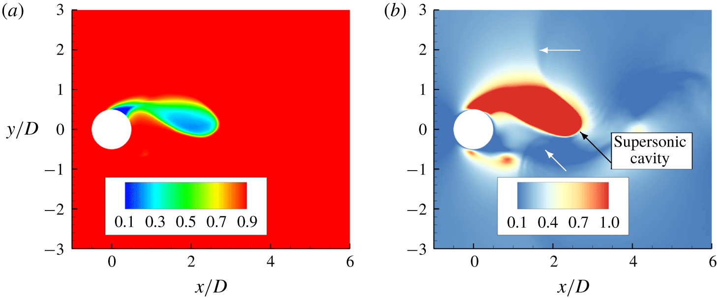For $\unicode[STIX]{x1D70E}=0.85$, instantaneous density contours showing the cavity region (figure 19a) and corresponding Mach number contours (figure 19b) indicate that the cavity is supersonic. It is noticeable that the pressure wave generated due to the collapse of the previously shed cavity (indicated by the white arrow), does not propagate through the cavity, as shown in figure 19(b), and instead travels through the surrounding subsonic liquid region. 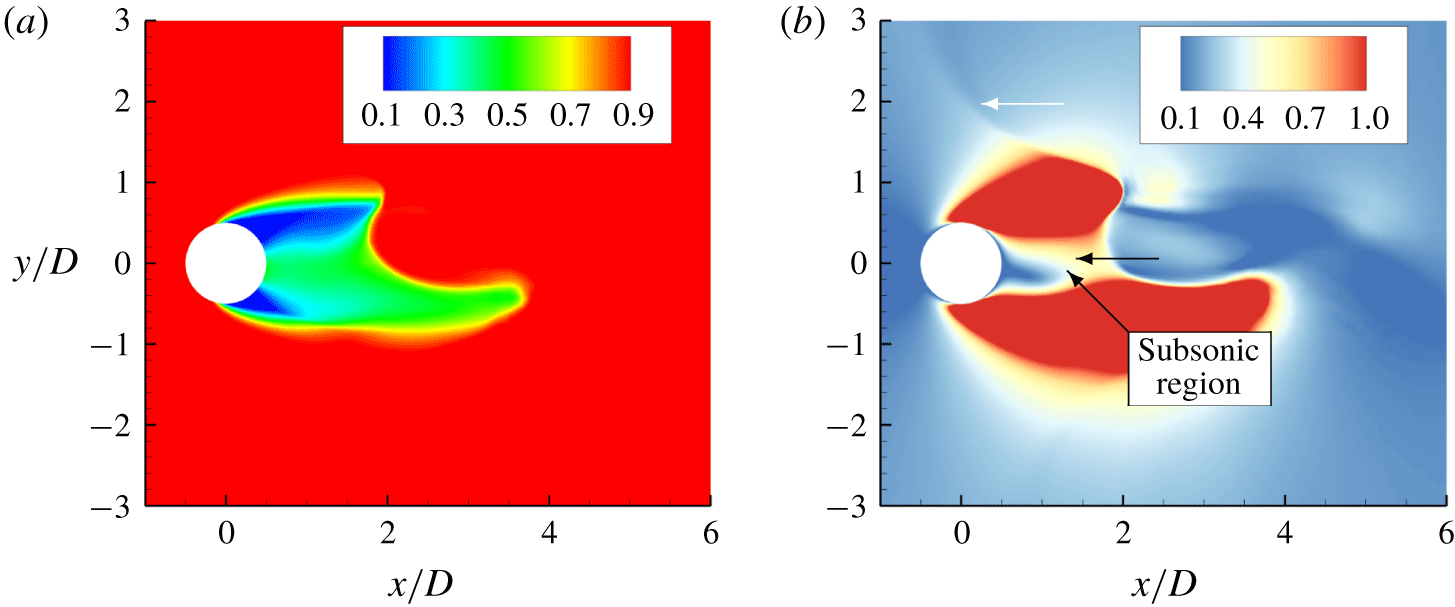In contrast, at $\unicode[STIX]{x1D70E}=0.7$, the cavity region surrounding the cylinder trailing edge and near wake is subsonic as shown in figure 20(a). The propagation of the shock wave through the cavity is indicated by the black arrow.

Figure 19.

Instantaneous density (a) and Mach number (b) contours of the attached cavity for $\unicode[STIX]{x1D70E}=0.85$.

Figure 20.

Instantaneous density (a) and Mach number (b) contours of the attached cavity for $\unicode[STIX]{x1D70E}=0.7$.

4.3.3 Effect of NCG on condensation shock

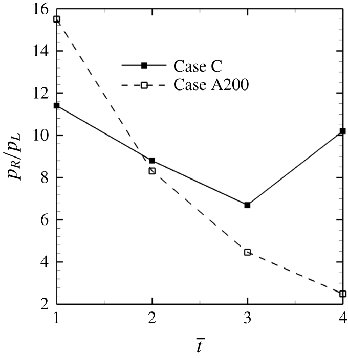
Section 4.3.1 demonstrated that, in the presence of NCG, the Mach number of the condensation shock decreases as it approaches the cylinder. Consequently, two condensation shock waves were necessary for complete condensation and detachment of the cavity. This section explains this weakening of the condensation shock as it travels in the presence of NCG. The strength of the condensation shock is characterized by the pressure ratio and is plotted in figure 21 for the instants of time mentioned in figure 17. It is evident that the pressure ratio monotonically decreases as the shock approaches the cylinder surface in the presence of NCG (case A200). The initial pressure ratio of 16 reduces to 2.5 near the cylinder trailing edge. Variation in the pressure ratio when NCG is absent (case C) is expected due to the finite rate of condensation; if the condensation rate is not strong enough to condense large portions of the vapour as the shock moves, some amount of uncondensed vapour remain after the passage of the shock decreasing its strength. In the cases considered here, the pressure rise observed across the condensation shock is much lower as compared to the pressure jump across the typical shock wave generated due to cavity collapse.

Figure 21.

Pressure ratio across a condensation shock for $\unicode[STIX]{x1D70E}=0.7$.

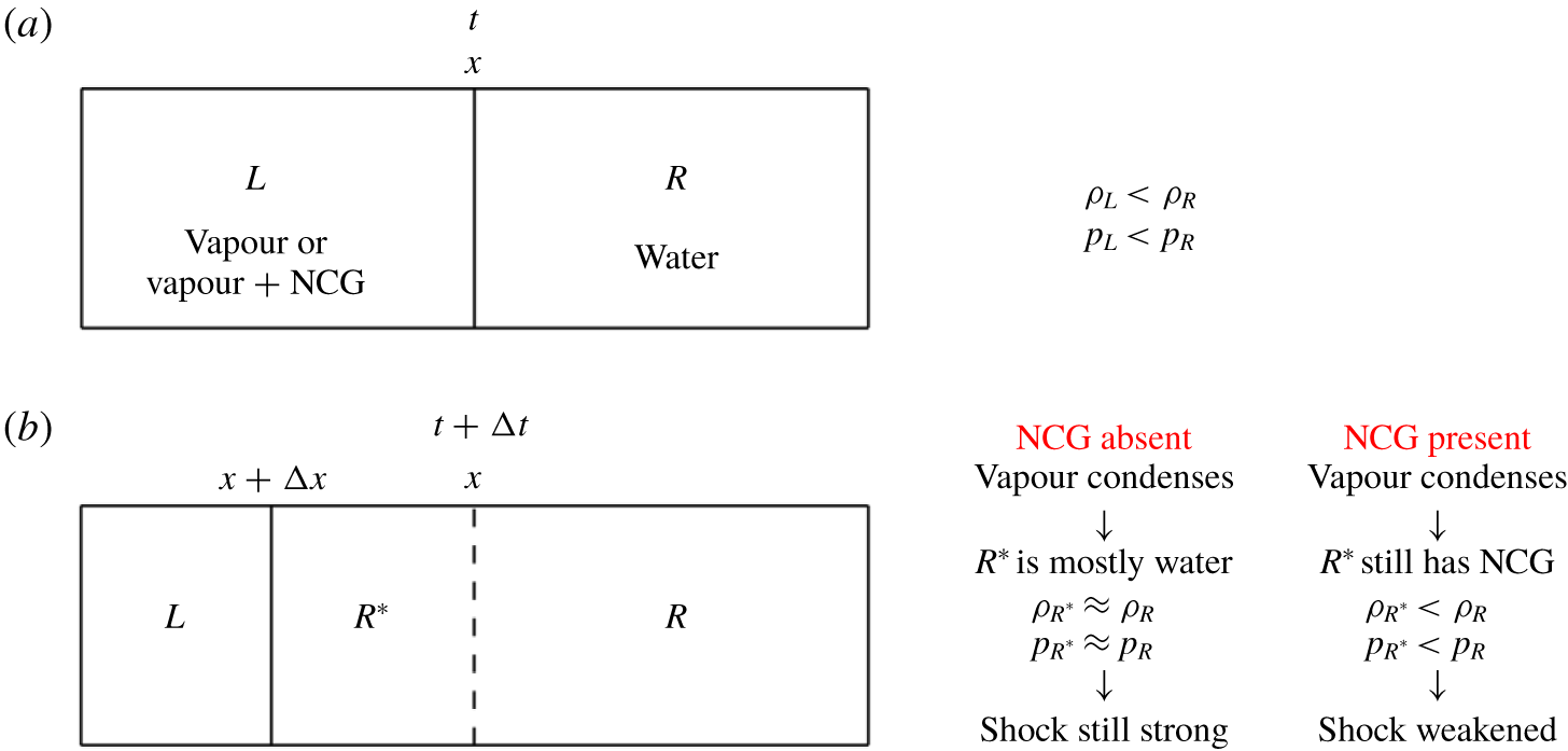
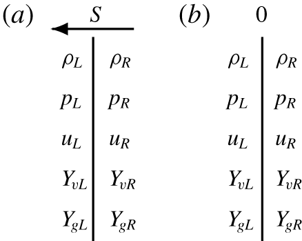
Reduction in the pressure ratio due to the presence of a gaseous phase behind the shock is explained by considering the typical setting of a condensation shock moving from water to a cavity consisting of a vapour/NCG mixture, as shown in figure 22(a). Density and pressure behind the shock ($\unicode[STIX]{x1D70C}_{R}$ and $p_{R}$) are higher than those ahead of the shock ($\unicode[STIX]{x1D70C}_{L}$ and $p_{L}$). At time $t+\unicode[STIX]{x0394}t$, the condensation shock moves through the cavity of vapour/gas mixture to $x+\unicode[STIX]{x0394}x$ creating region $R\ast$ behind the shock, as shown in figure 22(b). Now, the jump conditions are determined across the region $L$ and $R\ast$. Assuming that the vapour is completely condensed as the shock travels through the cavity; if the cavity consisted only of vapour, the region $R\ast$ behind the shock remains nearly the same as $R$ and is primarily water. In contrast to that, if the cavity also had NCG, the region $R\ast$ would have a mixture of water and NCG. Consequently, the overall density is reduced as compared to the original density of water ($\unicode[STIX]{x1D70C}_{R^{\ast }}<\unicode[STIX]{x1D70C}_{R}$), and using the jump conditions derived in (A 14) it can be shown that the pressure jump accordingly is also reduced ($p_{R^{\ast }}/p_{L}<p_{R}/p_{L}$). Hence, the condensation shock weakens as it propagates through a cavity that contains NCG. Subsequently, we consider the conditions at which condensation shock cease to exist as it weakens with the reduction in pressure ratio.

Figure 22.

Diagram for the example of a left-moving shock.

Figure 23.

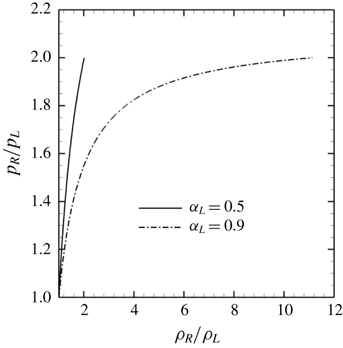
Pressure jump across condensation shock at sonic conditions for different density ratios and gaseous phase void fractions ahead of the shock.

For single-phase flows, the pressure ratio across the shock is determined uniquely using the shock Mach number (Toro Reference Toro1999). However, this is not the case for condensation shocks since multiple phases can be present on either side of the shock. Equation (A 15) derived in appendix A shows that the shock speed and consequently the shock Mach number are not uniquely related to the pressure ratio, they also depend on vapour/NCG mass fractions ahead and behind the shock and the resulting density difference. In contrast, the pressure and density ratio are equal to 1 at sonic conditions for single-phase flows. As an example, figure 23 shows the pressure jump plotted at sonic conditions across a condensation shock using the current system of equations and the jump conditions described by (A 14) for different total void fractions ahead of the front ($\unicode[STIX]{x1D6FC}_{L}$). It is clear that, in case of condensation shocks, the pressure jump is not unique at a given shock Mach number.

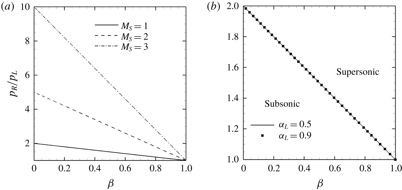
By combining the ratios of density and gaseous phase volume fraction into a single parameter ($\unicode[STIX]{x1D6FD}=(\unicode[STIX]{x1D6FC}_{R}/\unicode[STIX]{x1D6FC}_{L})/(\unicode[STIX]{x1D70C}_{R}/\unicode[STIX]{x1D70C}_{L})$) and plotting the resultant pressure ratio for different shock Mach numbers, figure 24(a) is obtained and equation (4.2) can be derived from it with a linear fit, assuming $u_{L}$ to be 0 for simplicity.

(4.2)

$$\begin{eqnarray}p_{R}/p_{L}=-M_{S}^{2}\unicode[STIX]{x1D6FD}+M_{S}^{2}+1.\end{eqnarray}$$

Figure 24.

Pressure ratio against different values of $\unicode[STIX]{x1D6FD}$ at different $M_{S}$ (a). Pressure ratio necessary for condensation shock (b).

At sonic conditions, the pressure ratio is simplified to

(4.3)

$$\begin{eqnarray}p_{R}/p_{L}=2-\unicode[STIX]{x1D6FD},\end{eqnarray}$$

and shown in detail in figure 24(b). From figure 24(b), it is evident that the results of figure 23 can collapse when plotted using (4.3). Figure 24(b) allows us to consider a parameter space for which the condensation front is supersonic. Note that in the single-phase limit ($\unicode[STIX]{x1D6FC}_{R}=\unicode[STIX]{x1D6FC}_{L}=1$), equation (2.5) reduces to the ideal gas equation of state and equation (4.3) suggests that $p_{R}/p_{L}=1$ and $\unicode[STIX]{x1D70C}_{R}/\unicode[STIX]{x1D70C}_{L}=1$ has to be identically satisfied at sonic conditions. The value of $\unicode[STIX]{x1D6FD}=0$ when the phase is completely liquid behind the shock. This suggests that the pressure ratio has to be greater than 2 for the condensation front propagating from the liquid ($\unicode[STIX]{x1D6FD}=0$) into a gaseous cavity to be supersonic. It is important to note, however, that if the phase behind the shock is not completely liquid ($\unicode[STIX]{x1D6FD}>0$), the pressure ratio for the occurrence of a supersonic Mach number can be less than 2. In the current simulations, although the pressure ratio across the condensation front reduces as it propagates through the cavity containing NCG, it remains greater than a factor of 2, indicating that the condensation front remains supersonic as it travels towards the cylinder. Since the state ahead of the shock is the attached cavity, we can conclude that, as long as the pressure ratio across the condensation shock does not drop to values below 2, the condensation shock will remain supersonic regardless of the amounts of gaseous phase inside the cavity.

4.4 LES of cavitating flow at $Re=3900$

LES of turbulent cavitating flow over a cylinder is performed at $Re=3900$ in both the cyclic and the transitional regimes, respectively at $\unicode[STIX]{x1D70E}=1.0$ and $\unicode[STIX]{x1D70E}=0.7$, using a low free-stream nuclei concentration (case A3900). As noted in appendix B, the temperature changes in the flow are negligible. Hence, we perform LES calculations using isothermal formulation.

4.4.1 Cyclic regime

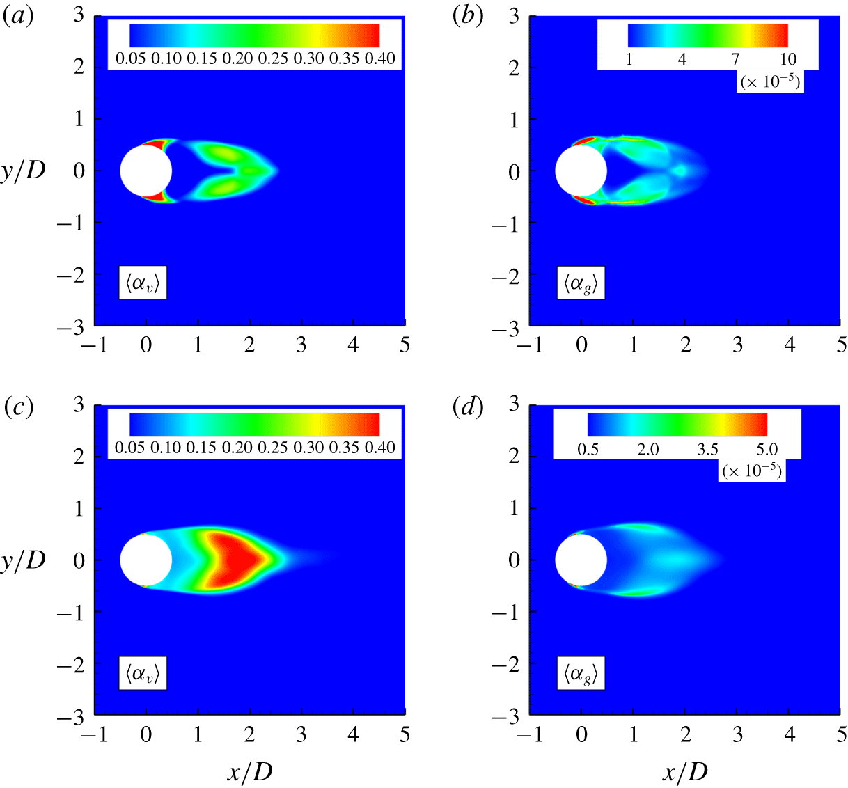
We consider a mean vapour and NCG volume fraction at $Re=3900$ and compare it to $Re=200$ (figure 25). At $Re=3900$, only a thin layer of vapour is observed at the cylinder surface as compared to the $Re=200$ (figure 25a,c). Also, at higher $Re$, more vapour is observed in the region of the near wake. At $Re=3900$, the incoming boundary layer is turbulent and confined close to the cylinder surface. This results in higher vorticity inside the Kármán vortices, leading to larger pressure drop and more vapour production in the wake. The mean volume fraction of NCG at $Re=3900$, however, is observed to be one order of magnitude lower than at $Re=200$ (figure 25b,d).

Figure 25.

Mean volume fractions at $Re=200$ ((a) vapour, (b) NCG) and $Re=3900$ ((c) vapour, (d) NCG).

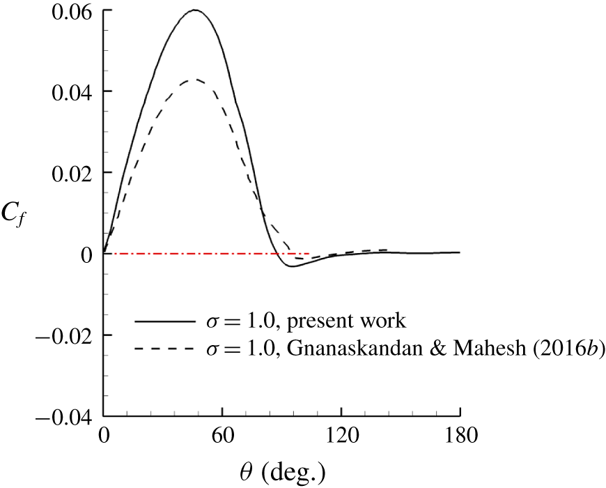
The skin friction coefficient is compared to the result from Gnanaskandan & Mahesh (Reference Gnanaskandan and Mahesh2016b) in figure 26. They studied the cyclic cavitation regime at $\unicode[STIX]{x1D70E}=1.0$ using free-stream nuclei concentration of 0.01 for vapour (case C of the current simulations). As noted for the laminar separation at $Re=200$, we observe that at $Re=3900$ the boundary-layer separation point moves upstream as compared to Gnanaskandan & Mahesh (Reference Gnanaskandan and Mahesh2016b) (figure 26). The difference between the separation points is approximately $10^{\circ }$, the same observed for $Re=200$. These results confirm the role of free-stream total void fraction on the location of boundary-layer separation.

Figure 26.

Skin friction coefficient at $Re=3900$. Red dashed line identifies $C_{f}=0$.

4.4.2 Transitional regime

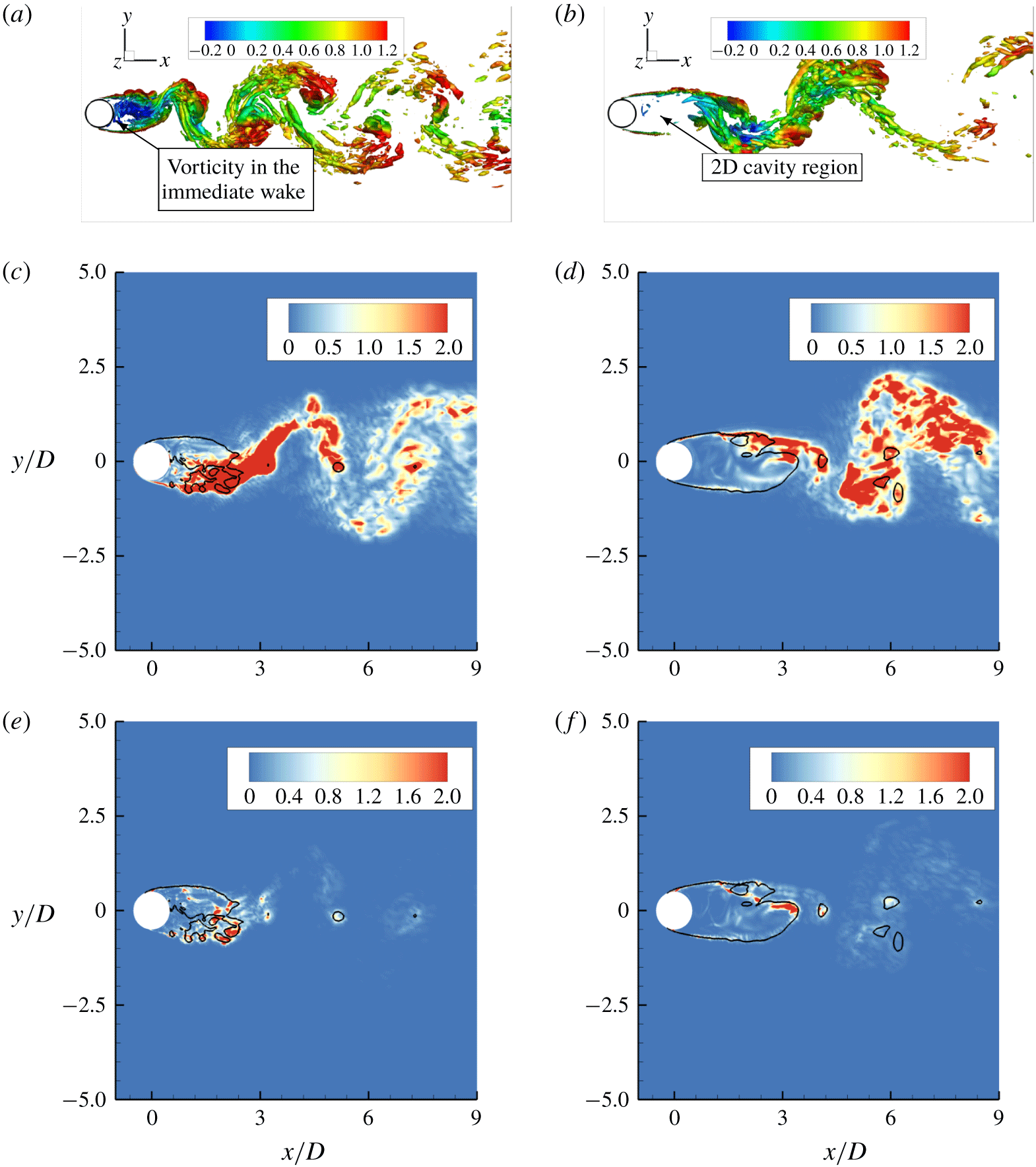
We noted that, in the transitional regime, flow cavitates over the entire aft body of the cylinder continuing into the regions in the immediate wake. Consequently, the grown cavity is observed to be nearly two-dimensional with negligible vorticity within the cavity (figure 27b). Figure 27(a,b) shows a comparison to the cyclic cavitation. In the cyclic regime, significant vorticity is observed in the immediate wake of the cylinder (figure 27a). Vortex stretching/tilting plotted in figure 27(c,d) confirms this distinction. In the transitional regime, a stable region of incoming shear layer is visible on the either side of the cylinder and the majority of stretching/tilting is observed following the cavity closure. Consequently, in the transitional regime, periodic shedding and breakdown of Kármán vortices are significantly altered. In addition, in the cyclic regime, due to the three-dimensionality of the flow, significant vorticity production is observed in the near wake by misaligned density gradients in the cavity region and the pressure gradients in the pressure waves generated by cavity collapse. In the transitional regime, vorticity production within the 2-D cavity is negligible, while vorticity production is observed in the cavity closure at the onset of three-dimensionality in the flow.

Figure 27.

Vortex transport for cyclic regime (a,c,e) and transitional regime (b,d,f). $Q$ criterion coloured by streamwise velocity (a,b), vorticity stretching/tilting (c,d) and baroclinic torque (e,f). Black lines indicate isosurface of total void fraction of $0.1$ and represent the cavity interface.

Figure 28.

Spanwise average of density contours showing the propagation of a condensation front at $\unicode[STIX]{x1D70E}=0.7$ and $Re=3900$. Time increases from left to right.

Figure 29.

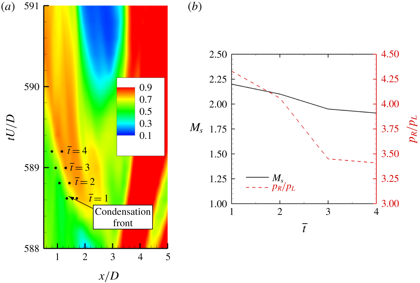
An $x$–$t$ plot of spanwise averaged density (a) and condensation front Mach number and pressure ratio (b) at $\unicode[STIX]{x1D70E}=0.7$ and $Re=3900$.

In the transitional regime, at $Re=200$, we observed that in the presence of NCG propagation of multiple condensation shocks leading to complete cavity detachment. The same is also observed at $Re=3900$ as illustrated in figure 28 using spanwise averaged density contours at multiple time instances. Compared to $Re=200$, the condensation front at $Re=3900$ is oriented more vertically rather than towards the cylinder trailing edge. Note the first front moving in the direction of the negative $y$-axis and the second front moving in the direction of the positive $y$-axis and also oriented towards the cylinder surface. Time evolution of condensation front propagation is shown using an $x$–$t$ diagram in figure 29(a), only the section front moving towards the cylinder surface is considered. Initial and final time instances of the propagation are displayed in figures 29(c) and 29(d). Mach number and the pressure ratio across the condensation front are computed at the time instances indicated in figure 29(a) and are displayed in figure 29(b). The condensation front moves at supersonic speeds at all the instances considered, and consequently this is a condensation shock wave. Also, note that the condensation shock is weakened as it propagates and approaches the cylinder surface, as indicated in figure 29 by reduction in the pressure ratio.

5 Summary

The numerical method of Gnanaskandan & Mahesh (Reference Gnanaskandan and Mahesh2015) to study cavitating flows based on a homogeneous mixture of water–vapour is extended to include NCG. Cavitating flow over a circular cylinder is studied for a range of $\unicode[STIX]{x1D70E}$ showing both cyclic and transitional cavitation regimes at different Reynolds numbers and with different amounts of free-stream vapour and gas volume fraction. NCG is introduced in the free stream as a free gas (prescribed in a similar way as vapour nuclei) and its effect on the flow field is discussed. In the cyclic regime, cavitation was observed in periodically shedding Kármán vortices; while in the transitional regime, the cavity shedding was observed due to propagating condensation shocks.

The value of $St$ based on cavity length, when plotted with $\unicode[STIX]{x1D70E}$, shows a peak just before the onset of condensation shock wave induced cavity shedding. Cavity shedding frequency obtained from the drag history showed similar behaviour in the presence of NCG. At $\unicode[STIX]{x1D70E}=0.85$ (near transition), however, FFT of the pressure history did not show a secondary peak due to low frequency detachment in the presence of NCG, suggesting its influence in delaying the transition to low frequency shedding behaviour. DMD used to investigate wake characteristics revealed that cavitation delays the first transition of the Kármán vortex street. Reduction in shedding frequency as $\unicode[STIX]{x1D70E}$ is lowered from non-cavitating to cavitating conditions is used to explain this behaviour.

It was observed that vapour and gas uniformly introduced in the free stream, distributed themselves differently in the wake of cylinder depending upon local flow conditions, particularly at lower cavitation numbers as the pressure in the wake dropped below vapour pressure. This was explained using $\unicode[STIX]{x1D70E}_{local}$, to distinguish vapour production due to phase change as compared to expansion of vapour or gas. Vapour and NCG distribution in the boundary layer suggested that cavitation as a mass transfer process only occurs inside a fine layer in the near-wall region, while the remaining boundary layer only undergoes expansion of both vapour and gas. Free-stream void fraction was shown to have a large impact on the mean gas volume fraction observed inside the cavity. However, mean vapour volume fraction seems relatively independent. The boundary-layer separation point for both laminar and turbulent flows was observed to move downstream as the free-stream volume fraction is increased.

Rankine–Hugoniot jump conditions were derived for the complete system. The shock speed obtained using the jump conditions is used to compute the Mach number of propagating condensation front to show that it is indeed supersonic for both $Re$ studied. It is however noted that the condensation shock propagates into a subsonic region of the cavity, based on local Mach numbers. In the presence of NCG, it was shown that the strength of the condensation shock reduces as it approaches the cylinder surface. This results in multiple condensation shocks being necessary for detachment of the cavity. Weakening of the shock strength in the presence of gas was due to a reduction in pressure ratio across the condensation shock as it approaches the cylinder surface. As the shock moves upstream towards the cylinder, it condenses the vapour along the way. However, the fact that it cannot condense the NCG resulted in a lower pressure behind the shock, which was shown using the jump condition. The conditions necessary for the occurrence of supersonic condensation front are then assessed using its pressure ratio.

At $Re=3900$, it was observed that the location of maximum vapour production in the cyclic regime is shifted from the cylinder surface to the immediate wake, with no major changes to the levels of volume fraction inside the cavity. The mean NCG volume fraction, however, reduces by an order of magnitude inside the cavity when compared to the mean values at $Re=200$. The growth of a nearly two-dimensional cavity in the transitional regime, significantly reduces vortex stretching and baroclinic torque from the values observed in the cyclic regime. Finally, it is observed that at $Re=3900$ for the transitional regime, the cavity detaches after the passage of a more vertically oriented condensation shock, different from the horizontally oriented shock at $Re=200$.

Acknowledgements

This work is supported by the United States Office of Naval Research under grant ONR N00014–17-1–2676 with Dr K.-H. Kim as the program manager. Computing resources were provided by the Minnesota Supercomputing Institute (MSI) and the High Performance Computing Modernization Program (HPCMP).

Declaration of interests

The authors report no conflict of interest.

Supplementary movies

Supplementary movies are available at https://doi.org/10.1017/jfm.2019.971.

Appendix A. Analysis of condensation shock using Rankine–Hugoniot jump conditions

Analysis of shock waves in bubbly flows of liquid–gas mixtures was considered by Campbell & Pitcher (Reference Campbell and Pitcher1958), who related shock propagation speed to the pressure in the high-pressure side of the shock, the density of the liquid and relative proportions of gas and liquid. They also showed negligible temperature rise across steady condensation shock waves. Here, we consider the current system of homogeneous mixture with both vapour and gas mass transport closed with the mixture equation of state and consider a left-moving shock (moving upstream of the flow direction) in a frame of reference moving with the shock as described in figure 30. The velocities in the moving reference frame are

(A 1a,b)

$$\begin{eqnarray}\hat{u} _{L}=u_{L}-S\quad \text{and}\quad \hat{u} _{R}=u_{R}-S.\end{eqnarray}$$

Here, $S$ is the shock speed; is used to indicate quantities in moving reference frame; ‘$L$’ and ‘$R$’ subscripts are used respectively for the quantities at the left and at the right of the shock. Since we are considering a left-moving shock, left and right sides of the shock are ahead and behind the shock respectively.

Figure 30.

Left-moving shock in a stationary frame of reference (a) and in a frame of reference moving with the shock (b).

The Rankine–Hugoniot jump conditions in a frame of reference moving with the shock are,

(A 2)

$$\begin{eqnarray}\displaystyle & \displaystyle \unicode[STIX]{x1D70C}_{R}\hat{u} _{R}=\unicode[STIX]{x1D70C}_{L}\hat{u} _{L}, & \displaystyle\end{eqnarray}$$

(A 3)

$$\begin{eqnarray}\displaystyle & \displaystyle \unicode[STIX]{x1D70C}_{R}\hat{u} _{R}^{2}+p_{R}=\unicode[STIX]{x1D70C}_{L}\hat{u} _{L}^{2}+p_{L}, & \displaystyle\end{eqnarray}$$

(A 4)

$$\begin{eqnarray}\displaystyle & \displaystyle \unicode[STIX]{x1D70C}_{R}\hat{u} _{R}(e_{R}+p_{R}/\unicode[STIX]{x1D70C}_{R}+\hat{u} _{R}^{2}/2)=\unicode[STIX]{x1D70C}_{L}\hat{u} _{L}(e_{L}+p_{L}/\unicode[STIX]{x1D70C}_{L}+\hat{u} _{L}^{2}/2), & \displaystyle\end{eqnarray}$$

(A 5)

$$\begin{eqnarray}\displaystyle & \displaystyle \unicode[STIX]{x1D70C}_{R}Yv_{R}\hat{u} _{R}=\unicode[STIX]{x1D70C}_{L}Yv_{L}\hat{u} _{L}\quad \text{and} & \displaystyle\end{eqnarray}$$

(A 6)

$$\begin{eqnarray}\displaystyle & \displaystyle \unicode[STIX]{x1D70C}_{R}Yg_{R}\hat{u} _{R}=\unicode[STIX]{x1D70C}_{L}Yg_{L}\hat{u} _{L}. & \displaystyle\end{eqnarray}$$

Here, subscripts $v$ and $g$ in (A 5) and (A 6) denote vapour and NCG respectively. Note that phase change between vapour and water is not explicitly modelled, however, its effects are implicitly calculated since the vapour mass fraction will have different values across the shock.

Applying (A 2) to (A 3) and (A 4) we have

(A 7)

$$\begin{eqnarray}\displaystyle & \displaystyle \hat{u} _{R}^{2}=\frac{\unicode[STIX]{x1D70C}_{L}}{\unicode[STIX]{x1D70C}_{R}}\frac{(p_{R}-p_{L})}{(\unicode[STIX]{x1D70C}_{R}-\unicode[STIX]{x1D70C}_{L})}, & \displaystyle\end{eqnarray}$$

(A 8)

$$\begin{eqnarray}\displaystyle & \displaystyle \hat{u} _{L}^{2}=\frac{\unicode[STIX]{x1D70C}_{R}}{\unicode[STIX]{x1D70C}_{L}}\frac{(p_{R}-p_{L})}{(\unicode[STIX]{x1D70C}_{R}-\unicode[STIX]{x1D70C}_{L})}\quad \text{and} & \displaystyle\end{eqnarray}$$

(A 9)

$$\begin{eqnarray}\displaystyle & \displaystyle e_{R}+p_{R}/\unicode[STIX]{x1D70C}_{R}+\hat{u} _{R}^{2}/2=e_{L}+p_{L}/\unicode[STIX]{x1D70C}_{L}+\hat{u} _{L}^{2}/2. & \displaystyle\end{eqnarray}$$

Substituting (A 7) and (A 8) into (A 9) we have an equation for the energy difference across the shock,

(A 10)

$$\begin{eqnarray}e_{R}-e_{L}=\frac{1}{2}\frac{(p_{R}+p_{L})(\unicode[STIX]{x1D70C}_{R}-\unicode[STIX]{x1D70C}_{L})}{\unicode[STIX]{x1D70C}_{R}\unicode[STIX]{x1D70C}_{L}}.\end{eqnarray}$$

From (2.5) and (2.4), the mixture internal energy can be written as

(A 11)

$$\begin{eqnarray}e=\frac{C_{vm}p^{2}+[C_{vm}+(1-Y_{v}-Y_{g})K_{l}]P_{c}p}{[\unicode[STIX]{x1D70C}(Y_{v}R_{v}+Y_{g}R_{g})(p+P_{c})+\unicode[STIX]{x1D70C}(1-Y_{v}-Y_{g})K_{l}p]},\end{eqnarray}$$

and can be simplified as

(A 12)

$$\begin{eqnarray}\displaystyle & \displaystyle e=\frac{p}{\unicode[STIX]{x1D70C}(\overline{\unicode[STIX]{x1D6FE}}-1)},\quad \text{where} & \displaystyle\end{eqnarray}$$

(A 13)

$$\begin{eqnarray}\displaystyle & \displaystyle \frac{1}{\overline{\unicode[STIX]{x1D6FE}}-1}=\frac{C_{vm}p+[C_{vm}+(1-Y_{v}-Y_{g})K_{l}]P_{c}}{[(Y_{v}R_{v}+Y_{g}R_{g})(p+P_{c})+(1-Y_{v}-Y_{g})K_{l}p]}. & \displaystyle\end{eqnarray}$$

Using (A 12) in (A 10) followed by algebraic simplification we obtain an equation for the density ratio across the shock as

(A 14)

$$\begin{eqnarray}\frac{\unicode[STIX]{x1D70C}_{R}}{\unicode[STIX]{x1D70C}_{L}}=\frac{\displaystyle \frac{p_{R}}{p_{L}}\frac{\overline{\unicode[STIX]{x1D6FE}}_{R}+1}{\overline{\unicode[STIX]{x1D6FE}}_{R}-1}+1}{\displaystyle \frac{p_{R}}{p_{L}}+\frac{\overline{\unicode[STIX]{x1D6FE}}_{L}+1}{\overline{\unicode[STIX]{x1D6FE}}_{L}-1}},\end{eqnarray}$$

with (A 1), (A 2), (A 8) and (A 14) an equation for the shock speed can be derived,

(A 15)

$$\begin{eqnarray}S=u_{L}-\sqrt{\frac{\displaystyle (p_{R}-p_{L})\left[\frac{p_{R}}{p_{L}}\frac{\overline{\unicode[STIX]{x1D6FE}}_{R}+1}{\overline{\unicode[STIX]{x1D6FE}}_{R}-1}+1\right]}{\displaystyle (\unicode[STIX]{x1D70C}_{R}-\unicode[STIX]{x1D70C}_{L})\left[\frac{p_{R}}{p_{L}}+\frac{\overline{\unicode[STIX]{x1D6FE}}_{L}+1}{\overline{\unicode[STIX]{x1D6FE}}_{L}-1}\right]}}.\end{eqnarray}$$

Note that in the single-phase limit with $Y_{g}=1$, $Y_{v}=0$ and $1-Y_{v}-Y_{g}=0$, equation (A 15) simplifies into the classical gasdynamics equation (e.g. Toro Reference Toro1999).

Appendix B. Temperature jump relation across a condensation shock

Is is known that temperature variations in hydrodynamic cavitation are mostly negligible due to the high specific heat capacity of a liquid. However, temperature variations are observed to increase in developed cavitation involving mass transfer in large cavities (Holl, Billet & Weir Reference Holl, Billet and Weir1975). Therefore, the propagation of a condensation shock might be expected to lead to larger temperature fluctuations. Here, we use results from the simulations at $Re=200$ and $\unicode[STIX]{x1D70E}=0.7$ along with an equation for the temperature ratio across the condensation shock, to show that temperature variation in this process is also negligible.

Temperature ratio across the condensation shock can be derived from the density relation given by (A 14) and the mixture equation of state (2.5). It is given by

(B 1)

$$\begin{eqnarray}\left.\begin{array}{@{}c@{}}\displaystyle \frac{T_{L}}{T_{R}}=\frac{\displaystyle \left[\frac{2b_{R}}{a_{R}}+1+\frac{p_{L}}{p_{r}}\right](p_{L}+P_{c})a_{R}}{\displaystyle \left[\frac{p_{R}}{p_{L}}+\frac{2b_{L}}{a_{L}}+1\right](p_{R}+P_{c})a_{L}},\quad \text{where}\\ \displaystyle a=(Y_{v}R_{v}+Y_{g}R_{g})(p+P_{c})+(1-Y_{v}-Y_{g})K_{l}p\quad \text{and}\\ \displaystyle b=C_{vm}p+[C_{vm}+(1-Y_{v}-Y_{g})K_{l}]P_{c}.\end{array}\right\}\end{eqnarray}$$

Note from (B 1) that considering different values of vapour and gas mass fraction for left and right implies that, although the temperature jump is of comparable magnitude to pressure ratio when having completely gaseous phases on both sides, the ratio is nearly unity in the presence of liquid. We investigate this by considering a scenario where shock is moving from water to a mixture of water–vapour–gas with increasing gaseous phase void fraction. Pressure in the liquid is considered to be 1 atm and pressure inside the mixture is chosen to be vapour pressure. This mimics the scenario of condensation shock propagating through the cavity. Temperature jump obtained from the equation (B 1) for increasing gaseous phase void fraction is plotted in figure 31. The figure shows that the temperature ratio for any amount of gaseous void fraction ahead of the shock is negligible. The maximum ratio in the plot is $T_{R}/T_{L}=1.005$ for $\unicode[STIX]{x1D6FC}_{L}=0.994$ (which is much higher than the maximum void fractions reached in practical applications). The same conclusions would hold even in the presence of some amount of gaseous void fraction mixed with the liquid behind the shock (not shown here).

Figure 31.

Temperature ratio across a condensation shock for different amounts of gaseous phase ahead of shock.

Figure 32.

Temperature ratio across a condensation shock for $\unicode[STIX]{x1D70E}=0.7$.

The isothermal behaviour of the condensation shock is confirmed in our simulations. Here, we obtain the temperature jump across the condensation shock observed for $\unicode[STIX]{x1D70E}=0.7$ at time instances mentioned in figure 17. Figure 32 shows the temperature ratio both in the presence and absence of gas. It is evident that the condensation shock in the current calculation is nearly isothermal.

References

Anantharamu, S. & Mahesh, K. 2019 A parallel and streaming dynamic mode decomposition algorithm with finite precision error analysis for large data. J. Comput. Phys. 380, 355–377.CrossRef Google Scholar

Arakeri, V. H. 1975 Viscous effects on the position of cavitation separation from smooth bodies. J. Fluid Mech. 68, 779–799.CrossRef Google Scholar

Beattie, D. R. H. & Whalley, P. B. 1982 Simple two-phase fractional pressure drop calculation method. Intl J. Multiphase Flow 8, 83–87.CrossRef Google Scholar

Bhatt, M. & Mahesh, K. 2018 Investigation of sheet to cloud transition due to the propagation of condensation fronts over a sharp wedge using large eddy simulations. In Proceedings of the 10th International Symposium on Cavitation. ASME.Google Scholar

Brandao, F., Bhatt, M. & Mahesh, K. 2018 Effects of non-condensable gas on cavitating flow over a cylinder. In Proceedings of the 10th International Symposium on Cavitation. ASME.Google Scholar

Briancon-Marjollet, L., Franc, J. P. & Michel, J. M. 1990 Transient bubbles interacting with an attached cavity and the boundary layer. J. Fluid Mech. 218, 355–376.CrossRef Google Scholar

Budich, B., Schmidt, S. & Adams, N. A. 2018 Numerical simulation and analysis of condensation shocks in cavitating flows. J. Fluid Mech. 838, 759–813.CrossRef Google Scholar

Campbell, I. J. & Pitcher, A. S. 1958 Shock waves in liquid containing gas bubbles. Proc. R. Soc. Lond. A 243 (1235), 534–545.Google Scholar

Chen, J. L., Xue, B., Mahesh, K. & Siepmann, J. I. 2019 Molecular simulations probing the thermophysical properties of homogeneously stretched and bubbly water systems. J. Chem. Engng Data 64 (9), 3755–3771.CrossRef Google Scholar

Durgin, W. W. & Karlsson, S. K. F. 1971 On the phenomenon of vortex street breakdown. J. Fluid Mech. 48, 507–527.CrossRef Google Scholar

Franc, J. P. & Michel, J. M. 2005 Fundamentals of Cavitation. Kluwer Academic.Google Scholar

Fry, S. A. 1984 Investigating cavity/wake dynamics for a circular cylinder by measuring noise spectra. J. Fluid Mech. 142, 187–200.CrossRef Google Scholar

Ganesh, H., Deijlen, L., Bhatt, A., Wu, J. & Ceccio, S. L. 2018 Cavitation dynamics in wakes of bluff bodies. In 32nd Symposium on Naval Hydrodyanmics.Google Scholar

Ganesh, H., Makiharju, S. A. & Ceccio, S. L. 2016 Bubbly shock propagation as a mechanism for sheet-to-cloud transition of partial cavities. J. Fluid Mech. 802, 37–78.CrossRef Google Scholar

Gnanaskandan, A. & Mahesh, K. 2015 A numerical method to simulate turbulent cavitating flows. Intl J. Multiphase Flow 70, 22–34.CrossRef Google Scholar

Gnanaskandan, A. & Mahesh, K. 2016a Large eddy simulation of the transition from sheet to cloud cavitation over a wedge. Intl J. Multiphase Flow 83, 86–102.CrossRef Google Scholar

Gnanaskandan, A. & Mahesh, K. 2016b Numerical investigation of near-wake characteristics of cavitating flow over a circular cylinder. J. Fluid Mech. 790, 453–491.CrossRef Google Scholar

Holl, J. W., Billet, M. L. & Weir, D. S. 1975 Thermodynamic effects on developed cavitation. J. Fluids Engng 97 (4).CrossRef Google Scholar

Hsiao, C.-T. & Chahine, G. L. 2005 Scaling of tip vortex cavitation inception noise with a bubble dynamics model accounting for nuclei size distribution. Trans. ASME-I-J. Fluids Engng 127 (1).CrossRef Google Scholar

Jahangir, S., Hogendoorn, W. & Poelma, C. 2018 Dyanmics of partial cavitation in an axisymmetric converging-diverging nozzle. Intl J. Multiphase Flow 106, 34–45.CrossRef Google Scholar

Jakobsen, J. K. 1964 On the mechanism of head breakdown in cavitating inducers. J. Basic Engng 86 (2), 291–305.CrossRef Google Scholar

Ji, B., Luo, X., Peng, X., Zhang, Y., Wu, Y. & Xu, H. 2010 Numerical investigation of the ventilated cavitating flow around an under-water vehicle based on a three-component cavitation model. J. Hydrodyn. 22 (6), 753–759.CrossRef Google Scholar

Jiang, H. & Cheng, L. 2019 Transition to the secondary vortex street in the wake of a circular cylinder. J. Fluid Mech. 867, 691–722.CrossRef Google Scholar

Karasudani, T. & Funakoshi, M. 1994 Evolution of a vortex street in the far wake of a cylinder. Fluid Dyn. Res. 14, 331–352.CrossRef Google Scholar

Karplus, H. B. 1957 Velocity of sound in a liquid containing gas bubbles. J. Acoust. Soc. Am. 29, 12–61.CrossRef Google Scholar

Kawakami, D. T., Gin, Q. & Arndt, R. 2005 Water quality and the periodicity of sheet/cloud cavitation. In Proceedings of FEDSM’05.Google Scholar

Kieffer, S. W. 1977 Sound speed in liquid–gas mixtures: water–air and water–steam. J. Geophys. Res. 82, 2895–2904.CrossRef Google Scholar

Kumar, P., Bakshi, S. & Chatterjee, D. 2017a Experimental investigation of cavitation behind a circular cylinder in cross-flow. J. Therm. Sci. Engng Appl. 9, 0310004.Google Scholar

Kumar, P., Chatterjee, D. & Bakshi, S. 2017b Experimental investigation of cavitating structures in the near wake of a cylinder. Intl J. Multiphase Flow 89, 207–217.CrossRef Google Scholar

Kunz, R., Boger, F., Stinebring, D. R., Chyczewski, T. S., Lindau, J. W., Gibeling, H. J., Venkateswaran, S. & Govindan, T. R. 2000 A preconditioned Navier–Stokes method for two-phase flows with application to cavitation. Comput. Fluids 29 (8), 849–875.CrossRef Google Scholar

Laberteaux, K. R. & Ceccio, S. L. 2001 Partial cavity flows. Part 1. Cavities forming on models without spanwise variation. J. Fluid Mech. 431, 1–41.CrossRef Google Scholar

Lagumbay, R. S.2006 Modeling and simulation of multiphase/multicomponent flows. PhD thesis, University of Colorado.Google Scholar

Lu, N. X., Bark, G. & Bensow, R. 2012 Introducing non-condensable gas in unsteady sheet cavitation modelling. In 15th Numerical Towing Tank Symposium.Google Scholar

Makiharju, S. A., Ganesh, H. & Ceccio, S. L. 2017 The dynamics of partial cavity formation, shedding and the influence of dissolved and injected non-condensable gas. J. Fluid Mech. 829, 420–458.CrossRef Google Scholar

Mithun, M. G., Koukouvinis, P. & Gavaises, M. 2018 Numerical simulation of cavitation and atomization using a fully compressible three-phase model. Phys. Rev. Fluids 3 (6), 064304.CrossRef Google Scholar

Orley, F., Trummler, T., Hickel, S., Mihatsch, M. S., Schmidt, S. J. & Adams, N. A. 2015 Large-eddy simulation of cavitating nozzle flow and primary jet break-up. Phys. Fluids 27, 086101.CrossRef Google Scholar

Park, N. & Mahesh, K.2007 Numerical and modeling issues in LES of compressible turbulence on unstructed grids. AIAA Paper 2007-722.CrossRef Google Scholar

Ramamurthy, A. S. & Bhaskaran, P. 1977 Constrained flow past cavitating bluff bodies. J. Fluids Engng 99 (4), 717–726.CrossRef Google Scholar

Rao, B. C. S. & Chandrasekhara, D. V. 1976 Some characteristics of cavity flow past cylindrical inducers in venturi. J. Fluids Engng 98 (3), 461–466.Google Scholar

Saito, Y., Takami, R., Nakamori, I. & Ikohagi, T. 2007 Numerical analysis of unsteady behavior of cloud cavitation around a NACA0015 foil. Comput. Mech. 40, 85–96.CrossRef Google Scholar

Schenke, S. & van Terwisga, T. J. C. 2017 Simulating compressibility in cavitating flow using incompressible mass transfer solver. In 5th International Symposium of Marine Propulsors.Google Scholar

Seo, J. H., Moon, Y. J. & Shin, B. R. 2008 Prediction of cavitation flow noise by direct numerical simulation. J. Comput. Phys. 227, 6511–6531.CrossRef Google Scholar

Singhal, A. K., Athavale, M. M., Li, H. & Jiang, Y. 2002 Mathematical basis and validation of the full cavitation model. J. Fluids Engng 124, 617–624.CrossRef Google Scholar

Toro, E. F. 1999 Riemann Solvers and Numerical Methods for Fluid Dynamics. Springer.CrossRef Google Scholar

Trummler, T., Freytag, L., Schmidt, S. J. & Adams, N. A. 2018 Large eddy simulation of a collapsing vapor bubble containing non-condensable gas. In Proceedings of the 10th International Symposium on Cavitation. ASME.Google Scholar

Varga, J. & Sebestiyen, G. 1965 Experimental investigation of some properties of cavitating flow. Period. Polytech. 9 (3), 243–254.Google Scholar

Vennig, J., Smith, S., Brandner, P., Giosio, D. & Pearce, B. 2017 The influence of nuclei content on cloud cavitation about a hydrofoil. In International Symposium on Transport Phenomena and Dynamics of Rotating Machinery.Google Scholar

White, F. M. 2006 Viscous Fluid Flow. McGraw-Hill.Google Scholar

Wu, X., Maheux, E. & Chahine, G. L. 2017 An experimental study on sheet to cloud cavitation. Exp. Therm. Fluid Sci. 83, 129–140.CrossRef Google Scholar

Yee, H. C., Sandham, N. D. & Djomehri, M. J. 1999 Low-dissipative high-order shock-capturing methods using characteristic-based filters. J. Comput. Phys. 150 (1), 199–238.CrossRef Google Scholar

Young, J. O. & Holl, J. W. 1966 Effects of cavitation on periodic wakes behind symmetric wedges. J. Basic Engng 88 (1), 163–176.CrossRef Google Scholar

Table 1.Constants for species viscosity.

Figure 1.Vapour pressure variation with temperature.

Figure 2.Speed of sound in water–vapour mixtures (a) and in water–NCG mixtures (b).

Figure 3.Line extracted along the vortex centreline showing absence of ‘non-monotonic behaviour’ with the modified switch.

Table 2.Cases showing flow conditions chosen for the problem.

Figure 4.Domain illustrating sponge layer and region of coarse mesh (not to scale).

Figure 5.Instantaneous total void fraction (vapour $+$ NCG volume fraction) contour for the cyclic regime (a) and for the transitional regime (b,c) for case B. See supplementary movie 1 for the cyclic regime and supplementary movie 2 for the transitional regime, available at https://doi.org/10.1017/jfm.2019.971.

Figure 6.Instantaneous solution indicating vortex shedding at $\unicode[STIX]{x1D70E}=1.0$ (a) and $\unicode[STIX]{x1D70E}=0.7$ (b) for case B. Lines indicate constant vorticity and coloured contours represent density.

Figure 7.Value of $St$ for different $\unicode[STIX]{x1D70E}$ based on the cylinder diameter (a) and cavity length (b). Non-dimensional pressure fluctuations are represented by red symbols in (b) for case A200 (▲), case B (●) and case C (▪). Cavity length normalized by cylinder diameter for different $\unicode[STIX]{x1D70E}$ (c).

Figure 8.(a) Pressure signal at $x=2.5D$ in the cylinder wake scaled with free-stream density and speed of sound at $\unicode[STIX]{x1D70E}=0.85$ and (b) fast Fourier transform (FFT) of the corresponding signal scaled with its maximum value for better visualization.

Figure 9.Most energetic modes coloured by spanwise vorticity at $\unicode[STIX]{x1D70E}=5.0$ (a), $\unicode[STIX]{x1D70E}=1.0$ (b) and $\unicode[STIX]{x1D70E}=0.85$ (c).

Figure 10.Vortex street coloured by density for $\unicode[STIX]{x1D70E}=5.0$ (a), $\unicode[STIX]{x1D70E}=1.0$ (b). White boxes indicate the region where the spacing ratio is computed.

Table 3.Cross-wake distance between different sign vortices $(h)$, longitudinal distance between same sign vortices $(a)$ and their ratio at two different wake positions for $\unicode[STIX]{x1D70E}=5.0$ and $\unicode[STIX]{x1D70E}=1.0$.

Figure 11.Modes corresponding to drag peak frequency at $\unicode[STIX]{x1D70E}=1.0$ (a) and $\unicode[STIX]{x1D70E}=0.7$ (b) for case A200, coloured with streamwise velocity.

Figure 12.Time averaged vapour and NCG volume fraction contours respectively at $\unicode[STIX]{x1D70E}=1$ (a,b) and $\unicode[STIX]{x1D70E}=0.7$ (c,d) for the case A200. White line in (c) indicates azimuthal position of $110^{\circ }$.

Figure 13.Cavitation inside the boundary layer at $\unicode[STIX]{x1D70E}=0.7$ and for case A200. Profiles taken at $110^{\circ }$ from the leading edge. (a) Azimuthal velocity profile (▫) with local cavitation number (▪) and (b) mean vapour (——) and NCG (– –) volume fractions.

Figure 14.Time averaged vapour and NCG volume fraction contours respectively at $\unicode[STIX]{x1D70E}=1$ (a,b) and $\unicode[STIX]{x1D70E}=0.7$ (c,d) for case B.

Figure 15.Skin friction at different $\unicode[STIX]{x1D70E}$ for case A200 (a) and at $\unicode[STIX]{x1D70E}=1.0$ for different cases (b). The dash red line represents $C_{f}=0$ and indicates the separation point.

Figure 16.Density contours showing the propagation of a condensation front in the absence (case C) (a,c) and presence (case A200) (b,d) of NCG.

Figure 17.An $x{-}t$ plot of density along the wake centreline for $\unicode[STIX]{x1D70E}=0.7$ when (a) NCG is absent (case C) and (b) present (case A200).

Figure 18.Mach number of condensation front for $\unicode[STIX]{x1D70E}=0.7$.

Figure 19.Instantaneous density (a) and Mach number (b) contours of the attached cavity for $\unicode[STIX]{x1D70E}=0.85$.

Figure 20.Instantaneous density (a) and Mach number (b) contours of the attached cavity for $\unicode[STIX]{x1D70E}=0.7$.

Figure 21.Pressure ratio across a condensation shock for $\unicode[STIX]{x1D70E}=0.7$.

Figure 22.Diagram for the example of a left-moving shock.

Figure 23.Pressure jump across condensation shock at sonic conditions for different density ratios and gaseous phase void fractions ahead of the shock.

Figure 24.Pressure ratio against different values of $\unicode[STIX]{x1D6FD}$ at different $M_{S}$ (a). Pressure ratio necessary for condensation shock (b).

Figure 25.Mean volume fractions at $Re=200$ ((a) vapour, (b) NCG) and $Re=3900$ ((c) vapour, (d) NCG).

Figure 26.Skin friction coefficient at $Re=3900$. Red dashed line identifies $C_{f}=0$.

Figure 27.Vortex transport for cyclic regime (a,c,e) and transitional regime (b,d,f). $Q$ criterion coloured by streamwise velocity (a,b), vorticity stretching/tilting (c,d) and baroclinic torque (e,f). Black lines indicate isosurface of total void fraction of $0.1$ and represent the cavity interface.

Figure 28.Spanwise average of density contours showing the propagation of a condensation front at $\unicode[STIX]{x1D70E}=0.7$ and $Re=3900$. Time increases from left to right.

Figure 29.An $x$–$t$ plot of spanwise averaged density (a) and condensation front Mach number and pressure ratio (b) at $\unicode[STIX]{x1D70E}=0.7$ and $Re=3900$.

Figure 30.Left-moving shock in a stationary frame of reference (a) and in a frame of reference moving with the shock (b).

Figure 31.Temperature ratio across a condensation shock for different amounts of gaseous phase ahead of shock.

Figure 32.Temperature ratio across a condensation shock for $\unicode[STIX]{x1D70E}=0.7$.

Brandao et al. supplementary movie 1

Fig 5(a). Instantaneous total void fraction contour for the cyclic regime for Case B.

Video 174.4 KB

Brandao et al. supplementary movie 2

Fig 5(b,c). Instantaneous total void fraction contour for the transitional regime for Case B.

Video 511.5 KB

Brandao et al. supplementary figure 1

Figure_1: Vapor volume fraction fluctuation for Case A200 at sigma=1.

File 306.7 KB

Brandao et al. supplementary figure 2

Figure_2: NCG volume fraction fluctuation for Case A200 at sigma=1.

File 261.2 KB

Brandao et al. supplementary figure 3

Figure_3: Average local cavitation number for Case A200 at sigma=1.

File 310.8 KB

Brandao et al. supplementary figure 4

Figure_4: Average velocity magnitude for Case A200 at sigma=1.

File 837.3 KB

Brandao et al. supplementary figure 5

Figure_5: Vapor volume fraction fluctuation for Case A200 at sigma=0.7.

File 392.7 KB

Brandao et al. supplementary figure 6

Figure_6: NCG volume fraction fluctuation for Case A200 at sigma=0.7.

File 253.2 KB

Brandao et al. supplementary figure 7

Figure_7: Average local cavitation number for Case A200 at sigma=0.7.

File 877.2 KB

Brandao et al. supplementary figure 8

Figure_8: Average velocity magnitude for Case A200 at sigma=0.7.

File 877.2 KB

Article contents

Numerical study of cavitation regimes in flow over a circular cylinder

Abstract

JFM classification

Information

1 Introduction

2 Physical model and numerical method

2.1 Homogeneous mixture approach

2.2 Numerical method

2.3 Modifications to the multiphase switch

3 Problem set-up

4 Results

4.1 Shedding characteristics

4.1.1 $St$ versus $\unicode[STIX]{x1D70E}$

4.1.2 Effect of NCG

4.1.3 Dynamic mode decomposition

4.2 Mean flow characteristics

4.2.1 Distribution of vapour and NCG in the cylinder wake

4.2.2 Cavitation inside the boundary layer

4.2.3 Effect of free-stream nuclei

4.3 Condensation shock

4.3.1 Shock Mach numbers

4.3.2 Cavity Mach numbers

4.3.3 Effect of NCG on condensation shock

4.4 LES of cavitating flow at $Re=3900$

4.4.1 Cyclic regime

4.4.2 Transitional regime

5 Summary

Acknowledgements

Declaration of interests

Supplementary movies

Appendix A. Analysis of condensation shock using Rankine–Hugoniot jump conditions

Appendix B. Temperature jump relation across a condensation shock

References

Brandao et al. supplementary movie 1

Brandao et al. supplementary movie 2

Brandao et al. supplementary figure 1

Brandao et al. supplementary figure 2

Brandao et al. supplementary figure 3

Brandao et al. supplementary figure 4

Brandao et al. supplementary figure 5

Brandao et al. supplementary figure 6

Brandao et al. supplementary figure 7

Brandao et al. supplementary figure 8

Save article to Kindle

Save article to Dropbox

Save article to Google Drive

Reply to: Submit a response

Your details

You have entered the maximum number of contributors

Conflicting interests