

Epidemiologic research indicates that licit and illicit drug use among young adults has declined in recent decades (Grucza, Bucholz, Rice, & Bierut, Reference Grucza, Bucholz, Rice and Bierut2008; Johnston, O'Malley, Bachman, & Schulenberg, Reference Johnston, O'Malley, Bachman and Schulenberg2010a, 2010b; Kerr, Greenfield, Bond, Ye, & Rehm, Reference Kerr, Greenfield, Bond, Ye and Rehm2009; National Survey on Drug Use and Health, 2005; Wagenaar & Toomey, Reference Wagenaar and Toomey2002). These trends generalize to both prevalence rates and individual amounts of use. This research, which focused on cross-sectional data of successive cohorts, is useful and efficient for many purposes but may not accurately represent cohort differences in developmental trajectories and within-person change. Despite historical declines in amounts of drug use, longitudinal evidence suggests that the rate of increase in individual amounts of drug use during the transition to adulthood has actually accelerated among more recent cohorts (Schulenberg, O'Malley, Bachman, & Johnston, Reference Schulenberg, O'Malley, Bachman, Johnston, Crockett and Silbereisen2000, 2006). Together, these lines of research suggest a cohort by age interaction whereby cohort effects are stronger for younger respondents and then become weaker as respondents age. Thus, although the evidence for an overall reduction in amounts of drug use among adolescents and young adults suggests encouraging trends, the reliance on cross-sectional comparisons across cohorts is likely masking a less sanguine trend—that the pace of individual increases (or growth rate) in use between adolescence and young adulthood has been accelerating among more recent cohorts.
To address the gap between the typical epidemiological emphasis on cohort variation in point estimates and the typical etiological emphasis on individual drug use trajectories, we focus on historical change in individual trajectories of drug use during the transition to adulthood. We consider scope and magnitude, subgroup differences, and possible mechanisms. Charting historical variation in trajectories of young adult drug use is essential to capturing the full range of contextual influences on the development of risky behavior during the transition to adulthood. It also may have practical implications for policymakers and practitioners. Excessive and escalating drug use in young adulthood is associated with short-term physical, socioemotional, and academic problems (Bondy, Reference Bondy1996; Engs, Diebold, & Hanson, Reference Engs, Diebold and Hanson1996; Everett, Lowry, Cohen, & Dellinger, Reference Everett, Lowry, Cohen and Dellinger1999; Hingson, Heeren, Zakocs, Kopstein, & Wechsler, Reference Hingson, Heeren, Zakocs, Kopstein and Wechsler2002), and with long-term drug use problems and other forms of psychopathology (Schulenberg & Maggs, Reference Schulenberg and Maggs2002; Vaillant, & Hiller-Sturmhofel, Reference Vaillant and Hiller-Sturmhofel1996).
The Monitoring the Future project (MTF; Johnston et al., Reference Johnston, O'Malley, Bachman and Schulenberg2010a) provides this study with national panel data from 29 consecutive cohorts of high school seniors (graduating classes from 1976 to 2004). We examine historical changes in individual growth rates of heavy drinking (i.e., consuming five or more drinks in a row) and marijuana use between the ages of 18 and 22, testing for both across- and within-cohort differences. We focus on heavy drinking and marijuana use because alcohol and marijuana are the two most common psychoactive drugs, and both heavy drinking, an indicator of alcohol misuse, and marijuana use are associated with social harm, economic costs, and an increased disease burden (Rehm et al., Reference Rehm, Ashley, Room, Single, Bondy and Ferrence1996, Reference Rehm, Rehn, Room, Monteiro, Gmel and Jernigan2003; Sturm, Reference Sturm2002; Tashkin, Reference Tashkin2005). We focus on use within a narrow band of time (i.e., last 2 weeks for heavy drinking and last 30 days for marijuana use) to better capture excessive amounts of use.
The present study also seeks to uncover mechanisms responsible for historical change in drug use trajectories. In particular, we examine whether historical variation in individual growth rate is the result of historical changes in the young adult distribution of social roles regarding college, marriage, and parenthood, all of which are related to individual growth in drug use (e.g., Bachman, Wadsworth, O'Malley, Johnston, & Schulenberg, Reference Bachman, Wadsworth, O'Malley and Johnston1997). Given that the individuation process (and the opportunities for personal exploration that it affords) is thought to be more prolonged among today's young adults (Arnett, Reference Arnett2000; Bynner, Reference Bynner2005; Cote, Reference Cote2000; Settersten & Ray, Reference Settersten and Ray2010), we examine whether historical variation in individual growth rate is more sizable among subgroups who are traditionally afforded the most opportunities for exploration: those who go to college and those who live away from home.
Known Cohort Differences in Levels of Drug Use During the Transition to Adulthood
Levels of general alcohol use, heavy drinking, and marijuana use among high school seniors declined between the late 1970s and the early 2000s (Johnston et al., Reference Johnston, O'Malley, Bachman and Schulenberg2010a, Reference Johnston, O'Malley, Bachman and Schulenberg2010b). Their prevalence of annual, 30-day, and daily use declined between 25% and 45%, with declines generally higher for marijuana (Johnston et al., Reference Johnston, O'Malley, Bachman and Schulenberg2010a). Use declined among young adult respondents as well, though the size of the declines was less pronounced (Johnston et al., Reference Johnston, O'Malley, Bachman and Schulenberg2010b).
However, the pace of decline in use has not been constant across the last three decades. Rather than a constant broad-based macrotrend in drug use, there have been a series of shorter-term microtrends likely due to more proximal historical events and fluctuations in factors linked to drug use. For example, due to changes in federal policy, between 1985 and 1987, 31 states (including the District of Columbia) increased their minimum legal drinking age from age 18, 19, or 20 to age 21 (Hedlund, Ulmer, & Preusser, Reference Hedlund, Ulmer and Preusser2001; Wagenaar & Toomey, Reference Wagenaar and Toomey2002). The level of alcohol use among high school seniors and those aged 19 to 29 declined sharply between the late 1980s and the mid-1990s, with much slower declines in the years before and after this period (Johnston et al., Reference Johnston, O'Malley, Bachman and Schulenberg2010b). Declines in level of alcohol use were also evident, though less pronounced, in states that maintained a minimum drinking age of 21 and therefore are not entirely attributable to changes in minimum legal drinking age (O'Malley & Wagenaar, Reference O'Malley and Wagenaar1991). Microtrends in the level of marijuana use among high school seniors and young adults aged 19 to 29 followed a somewhat different pattern. The level of marijuana use among high school seniors and young adults aged 19 to 29 declined modestly but steadily between the late 1970s and early 1990s, increased sharply between the early and late 1990s, and then declined somewhat thereafter (Johnston et al., Reference Johnston, O'Malley, Bachman and Schulenberg2010a, Reference Johnston, O'Malley, Bachman and Schulenberg2010b).
Switching Focus From Level Differences to Growth Differences
Little attention has been given to how these historical shifts relate to individual trajectories of drug use (i.e., cohort by age interaction). Analyses of MTF longitudinal data across a limited set of cohorts raise new questions as the data suggest some acceleration in growth in heavy drinking and marijuana use among more recent cohorts (Schulenberg et al., Reference Schulenberg, O'Malley, Bachman, Johnston, Crockett and Silbereisen2000, Reference Schulenberg, O'Malley, Bachman, Johnston, Settersten, Furstenberg and Rumbaut2006). Is the acceleration across cohorts linear, consistent with a macrotrend, or nonlinear, consistent with the microtrends for point estimates discussed above? In addition, to what extent does the acceleration in growth “wash out” or negate historical declines in age 18 drug use? If the historical declines in age 18 use co-occur with more rapid increases in use between the ages of 18 and 22, then the age 22 historical declines in use should be of lower magnitude than the age 18 historical declines. To address this possibility, we also examine historical variation in the levels of age 22 drug use. We focus on drug use at age 22 because the level of heavy drinking peaks at this age (Bachman et al., Reference Bachman, Wadsworth, O'Malley and Johnston1997; Chen & Kandel, Reference Chen and Kandel1995; Johnston et al., Reference Johnston, O'Malley, Bachman and Schulenberg2010b; Muthén & Muthén, Reference Muthén and Muthén2000; O'Malley, Bachman, & Johnston, Reference O'Malley, Bachman and Johnston1988), while the level of marijuana use, which peaks around age 21, is still at near peak level (Chen & Kandel, Reference Chen and Kandel1995; Johnston et al., Reference Johnston, O'Malley, Bachman and Schulenberg2010b; Substance Abuse and Mental Health Services Administration, 2005). In addition, age 22 is the youngest age at which all members of all cohorts in the MTF are of legal drinking age.
Why Steeper Slopes?
To the extent that the individual trajectories of drug use during the transition to adulthood have steepened upward in more recent years, attention to mechanisms is needed. In research focused on the transition to adulthood, both psychological models, such as Arnett's (Reference Arnett2000) theory of emerging adulthood, and sociological approaches (Cote & Bynner, Reference Cote and Bynner2008; Hendry & Kloep, Reference Hendry and Kloep2007; Settersten & Ray, Reference Settersten and Ray2010; Shanahan, Reference Shanahan2000) highlight the interaction of individual factors, such as personal agency, and societal factors, such as social structure, in the creation of individualized life courses. Both perspectives also acknowledge that today the transition to adulthood is longer in duration and less standardized than it used to be (Arnett, Reference Arnett2000; Shanahan, Reference Shanahan2000). Two manifestations of the lengthening and destandardization of the transition to adulthood are historical changes in the young adult distribution of social roles and the duration and structure of the individuation process, both of which might contribute to historical variation in individual trajectories of young adult drug use.
Changes in the distribution of social roles
With the lengthening of the transition to adulthood comes the delay of adult roles and responsibilities such as marriage, a full-time career, and parenthood. Compared to the past, greater proportions of today's young adults are single (Arnett, Reference Arnett2000; Clark, Reference Clark2007; White, Reference White, Booth, Crouter and Shanahan1999), are childless (Arnett & Taber, Reference Arnett and Taber1994; Clark, Reference Clark2007) and pursue higher education (Johnston et al., Reference Johnston, O'Malley, Bachman and Schulenberg2010b; US Department of Education, 1996). Each of these social role statuses, relative to being married (Bachman et al., Reference Bachman, Wadsworth, O'Malley and Johnston1997; Powers, Rodgers, & Hope, Reference Powers, Rodgers and Hope1999), being a parent (Bachman et al., Reference Bachman, Wadsworth, O'Malley and Johnston1997), or working full time (Bachman et al., Reference Bachman, Wadsworth, O'Malley and Johnston1997; Slutske, Reference Slutske2005), is associated with greater individual increases in drug use during the transition to adulthood. Thus, the historical increase in young adult drug use growth rates may be, at least in part, due to the fact that subgroups of the young adult population that traditionally report greater individual increases in drug use have, over time, come to comprise a greater proportion of the young adult population.
A longer and less structured individuation process
Though the theory of emerging adulthood places greater emphasis on the role of personal agency and self-directed exploration while sociological approaches place greater emphasis on the role of social structure, both perspectives recognize that a key consequence of postponing adult commitments is a prolonged period of individuation that is unstructured, potentially anomic, and marked by exploration, instability, and freedom (Arnett, Reference Arnett2000, Reference Arnett, Arnett and Tanner2006; Cote, Reference Cote2000; Cote & Bynner, Reference Cote and Bynner2008; Hendry & Kloep, Reference Hendry and Kloep2007; Hill & Yeung, Reference Hill, Yeung, Booth, Crouter and Shanahan1999). Quite separate from the changing distribution of social roles (e.g., there are more of certain types of young adults today, the types that report greater individual increases in drug use) are the changing demands and structures of young adulthood (e.g., among young adults sharing similar demographics and backgrounds, the social landscape today is different from prior ones). To the extent that the delay of adultlike responsibilities, schedules, and priorities results in a prolonged and less structured period of individuation, the higher levels of exploration and experimentation that this altered period of individuation affords may translate into higher amounts of drug use, which are linked to experimentation and lack of social constraints (Bachman et al., Reference Bachman, Wadsworth, O'Malley and Johnston1997; Valliant & Scanlan, 1996). To the extent that this is the case, cohort differences in the individuation process may have contributed to cohort differences in individual trajectories of drug use.
If historical increases in opportunities for exploration and experimentation have contributed to the acceleration of drug use growth rates among recent cohorts of young adults, then cohort differences in drug use growth rates may be most evident among those going to college and living away from home. Relative to other young adults, daily constraints are lower and opportunities for exploration are higher among those going to college and living away from home (Bachman et al., Reference Bachman, Wadsworth, O'Malley and Johnston1997; Goldscheider & Goldscheider, Reference Goldscheider and Goldscheider1999; White, Fleming, Kim, Catalano, & McMorris, Reference White, Fleming, Kim, Catalano and McMorris2008). It stands to reason that within these subgroups of the young adult population, among whom opportunities for exploration and experimentation are particularly high, historical increases in opportunities for exploration and experimentation are also the highest.
Purposes of the Study
Our first aim is largely descriptive and seeks to clarify the magnitude and scope of historical variation in young adult drug use across the last three decades. Therefore, Building on Schulenberg et al. (Reference Schulenberg, O'Malley, Bachman, Johnston, Crockett and Silbereisen2000, Reference Schulenberg, O'Malley, Bachman, Johnston, Settersten, Furstenberg and Rumbaut2006) we examine in greater detail cohort differences in the age 18–22 growth rates and the age 22 levels of heavy drinking and marijuana use across the last three decades, and we examine whether cohort differences in the age 18–22 growth rates and the age 22 levels of heavy drinking and marijuana use are nonlinear and consistent with known microtrends in the age 18 levels. Our second aim seeks to uncover the mechanisms responsible for historical variation in individual trajectories of young adult drug use across the last three decades. We examine whether changes in the distribution of social roles account for historical variation and whether historical variation is more pronounced within certain social roles, with a focus on college attendance and young adult living arrangements. To examine the contribution of these mechanisms more directly, we control for minimum legal drinking age and race. Both are related to young adult drug use (Bachman et al., Reference Bachman, Wadsworth, O'Malley and Johnston1997; Wagenaar & Toomey, Reference Wagenaar and Toomey2002). The prevalence or mean rate of each has also fluctuated across the last three decades (Hobbs & Stoops, Reference Hobbs and Stoops2002; Wagenaar & Toomey, Reference Wagenaar and Toomey2002). Finally, due to known gender differences in young adult drug use, with males reporting higher levels of use as well as larger individual increases in use (Bachman et al., Reference Bachman, O'Malley, Schulenberg, Johnston, Bryant and Merline2002), we examine the above separately for each gender.
Methods
Respondents and procedure
MTF is an ongoing national study of the epidemiology and etiology of drug use among adolescents and adults (Bachman, Johnston, O'Malley, & Schulenberg, Reference Bachman, Johnston, O'Malley and Schulenberg2006; Johnston et al., Reference Johnston, O'Malley, Bachman and Schulenberg2010a). Beginning in 1975, large nationally representative samples of approximately 16,000 Grade 12 students were drawn from about 135 public and private schools each year (Johnston et al., Reference Johnston, O'Malley, Bachman and Schulenberg2010a, Reference Johnston, O'Malley, Bachman and Schulenberg2010b). Beginning with the class of 1976, approximately 2,400 respondents were randomly selected for biennial follow-up from each cohort through mail surveys, with one random half being surveyed 1 year after high school and the other random half being surveyed 2 years after high school; each half was followed biennially thereafter (the two random halves of each cohort are combined in these analyses). Respondents who reported illicit drug use at baseline were oversampled for follow-up.
In the present study we focused on the first three waves of the MTF panel data. Respondents were, on average, 18 years old at Wave 1, 19 to 20 years old at Wave 2, and 21 to 22 years old at Wave 3. The retention rate was 68% between Waves 1 and 2, 94% between Waves 2 and 3, and 65% between Waves 1 and 3. For the purposes of this study, analyses were limited to those respondents from the 1976–2004 cohorts of high school seniors who provided data at Wave 2, when data on social roles and living arrangements were first collected (N = 47,704). Attrition analyses indicated that compared to those excluded from the present study, those included were more likely to be female, to be white, to report a higher high school grade point average, to have more educated parents, and to report lower senior year heavy drinking and marijuana use. These analyses also indicated that attrition rates were slightly higher among recent cohorts. Though statistically significant, the effects of attrition were small in magnitude (i.e., R 2 = 0.02 for high school grade point average, R 2 < 0.005 for all other variables). Data extend until 2007/2008, when the most recent cohort of high school seniors was aged 21/22. (After adjusting for oversampling of drug users, the weighted N = 38,926.) Among those included in analyses, missingness was modestFootnote 1 (3.28% at Wave 1, 0.53% at Wave 2, and 19.14% at Wave 3). In order to maximize the data and include all possible cases, we used full information maximum likelihood estimation (Arbuckle, Reference Arbuckle, Marcoulides and Schumacker1996), a missing data algorithm available within Mplus (Muthén & Muthén, Reference Muthén and Muthén1998–2009).
Measures
Drug use
A single ordinal item was used to assess occasions of heavy drinking, operationalized as 5 or more drinks in a row in the past 2 weeks. Item responses included 1 (never), 2 (once), 3 (twice), 4 (3–5 times), 5 (6–9 times), and 6 (10 or more times). Occasions of marijuana use over the last 30 days was based on a single item, with responses of 1 (0 occasions), 2 (1–2 occasions), 3 (3–5 occasions), 4 (6–9 occasions), 5 (10–19 occasions), 6 (20–39 occasions), and 7 (40 or more occasions). Both drug use items were self-report.
Cohort measures
The measure cohort year ranged from 0 to 28 and was based on the year that respondents were seniors in high school (i.e., 1976 seniors = 0, 1977 seniors = 1, and so forth). This measure was used to examine linear trends in young adulthood drug use across the 1976–2004 cohorts. In addition, to examine microtrends in patterns of young adult drug use across cohorts, we broke the cohorts into the following three microtrend groups for heavy drinking: 1976–1986, 1987–1993, and 1994–2004. For marijuana use we broke the cohorts into the following three microtrend groups: 1976–1991, 1992–1997, and 1998–2004. The groupings were based on known microtrends in levels of age 18 heavy drinking and marijuana use described earlier (Johnston et al., Reference Johnston, O'Malley, Bachman and Schulenberg2010a).
Social roles
We dichotomized Wave 2 indicators of parental status, marital status, and college status. All indicators were self-report. For parental status, all those who had one or more children were coded as 1, and all those with no children were coded as 0. For marital status, all those who were married were coded as 1, and all those who were single, divorced, separated, or engaged were coded as 0. For college status, those who were attending a 4-year college full time were coded as 1, and all others, including those attending 2-year colleges (i.e., community colleges and vocational schools) and those attending any type of college part time, were coded as 0. We focused on those attending a 4-year college full time for two reasons. First, the relation between college attendance and individual increases in drug use is strongest among those enrolled in 4-year colleges (Douglas et al., Reference Douglas, Collins, Warren, Kann, Gold and Clayton1997) and those attending college full time (Bachman et al., Reference Bachman, Wadsworth, O'Malley and Johnston1997). Second, attending a 2-year college or attending college part time versus attending a 4-year college full time does not provide as many opportunities (in terms of both academics and social interactions) for exploration and experimentation (Davies & Casey, Reference Davies and Casey1999). For example, relative to full-time college students, those attending college part time are also more likely to work full time, drop out of school, and be “nontraditional” students with their own families (Bailey et al., Reference Bailey, Leinbach, Scott, Alfonso, Kienzl and Kennedy2003; Hearn, Reference Hearn1992; Horn & Berktold, Reference Horn and Berktold1998; Kane & Rouse, Reference Kane and Rouse1999). With the addition of being more likely to attend college part time and pursue vocational degrees, the same is true for those attending 2-year colleges relative to those attending 4-year colleges (Bailey et al., Reference Bailey, Leinbach, Scott, Alfonso, Kienzl and Kennedy2003; Horn & Berktold, Reference Horn and Berktold1998; Kane & Rouse, Reference Kane and Rouse1999). For college status by living arrangements, four categories were formed: in college/living away from parents, in college/living with parents, not in college/living away from parents, and not in college/living with parents. The measure for living arrangements was based on a single item.
Instability in social roles and living arrangements
We created Wave 3 measures of parental status, marital status, college status, and living arrangements using the same procedures we used to create the Wave 2 measures. The concordance rates for parental status, marital status, college status, and living arrangements across Waves 2 and 3 were 93%, 90%, 84%, and 74%, respectively. Previous research suggests that instability in these factors during young adulthood is related to within-cohort differences in drug use (e.g., Bachman et al., Reference Bachman, Wadsworth, O'Malley and Johnston1997; Schulenberg et al., Reference Schulenberg, O'Malley, Bachman, Johnston, Settersten, Furstenberg and Rumbaut2006). Because our primary aim is the examination of between-cohort differences in drug use, we do not further explore the influence of instability in social roles on within-cohort differences in drug use. Instead, while examining the relation between Wave 2 social roles and between-cohort differences in drug use, we control for the modest amount of instability in social roles across Waves 2 and 3. In order to do so, we created instability dummy variables that denote instability in these factors across Wave 2 and Wave 3. We include these dummy variables as control variables when necessary.
Key control variables
For race, all those who self-identified as European American were coded as 1, and all others were coded as 0. Minimum legal drinking age was based on self-reported state residency at Waves 1, 2, and 3, as well as data on state-level changes in minimum drinking age compiled by others (Hedlund et al., Reference Hedlund, Ulmer and Preusser2001; O'Malley & Wagenaar, Reference O'Malley and Wagenaar1991; Wagenaar & Toomey, Reference Wagenaar and Toomey2002). Based on these data, we determined each respondent's state's minimum legal drinking age at Waves 1, 2, and 3. Where possible, we allowed for changes in state residency across waves. However, prior to 1987, state of residency was asked at Wave 1 only. As a result, prior to 1986/1985Footnote 2 state residency data at Wave 2 were unavailable, and prior to 1984/1983 state residency data at Wave 3 were unavailable. When unavailable, state of residency at Waves 2 and 3 was based on state of residency at Wave 1. To highlight cohort (i.e., between-person) differences, we averaged each respondent's minimum legal drinking age at Waves 1, 2, and 3. We then subtracted the result from 21, producing a measure that allowed us to control for the influence of minimum legal drinking ages below the age of 21.
Results
After presenting preliminary analyses, we examine for our first aim: the magnitude of the historical variation in young adult drug use across the last three decades (i.e., macrotrends) and whether that historical variation is nonlinear and consistent with known microtrends of age 18 use. For our second aim, focusing on mechanisms potentially responsible for historical variation in drug use, we examine the extent to which historical changes in the distribution of social roles account for historical variation and the extent to which the size of historical variation differs across college status and living arrangements. All analyses were conducted with Mplus Version 5.2 (Muthén & Muthén, Reference Muthén and Muthén1998–2009). Due to space constraints, fit indices are not presented for each model, though in every case the comparative fit index was greater than 0.98 and the root mean square error of approximation was less than 0.03, suggesting that fit was very good for each model (McDonald & Ringo Ho, Reference McDonald and Ringo Ho2002). Because drug use typically shows a positively skewed distribution, all analyses utilize a maximum likelihood estimator that is robust to nonnormality. We used chi-square difference tests (Kline, Reference Kline1998, p. 133) to determine group differences.
Preliminary analyses
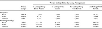
As expected, across cohort year, full-time college attendance increased while the marriage rate decreased (more so for females); the rate of parenthood remained steady (results not tabled). The sample was predominantly of European American descent (77.74%). Weighted frequencies and percentages of gender and the four college status by living arrangement groups are listed in Table 1.
Weighted frequencies and percentages by gender and by college status and living arrangements

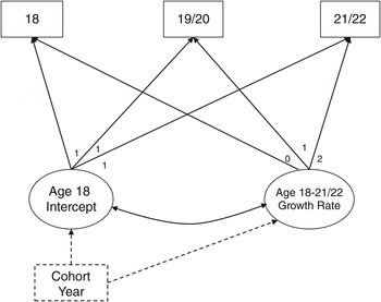
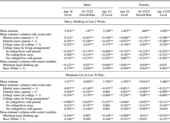
Though the paper's focus is on cohort differences in drug use, we examined how drug use in the aggregate sample (all cohorts combined) related to young adult social roles and the study's key control variables (Table 2). Using the baseline age 18–21/22 growth model in Figure 1, we estimated the age 18 level and the age 18–21/22 growth rate for both heavy drinking and marijuana use. We estimated the age 21/22 level of use in a separate model using the meanstructure analysis command in Mplus (Muthén & Muthén, Reference Muthén and Muthén1998–2009). To estimate the relation between the age 18 level of use and the age 18–21/22 growth rate and each young adult social role and key control variable, we included each social role and key control variable as an exogenous predictor of each drug use factor in the baseline growth model. In separate analyses, we examined the relation between the age 21/22 level of use and each young adult social role and key control variable by including the same set of exogenous predictors. All drug use estimates were of the expected magnitudes, and all relations were in the expected directions. In addition, for both heavy drinking and marijuana use, a higher minimum legal drinking age was negatively related to the age 18 and the age 21/22 levels of use. For heavy drinking, in particular, a higher minimum legal drinking age was also positively related to the age 18–21/22 growth rate.
Baseline and cohort year drug use growth models. The solid portion of the model represents the baseline age 18–21/22 growth model. The dashed and solid portions of the model combined represent the cohort year age 18–21/22 growth model.

Mean estimates of young adult drug use and their relation with Wave 2 (age 19/20) social roles and control variables

Note: All estimates are unstandardized.
aReference group is those in college living away from parents.
*p < .05. **p < .01.
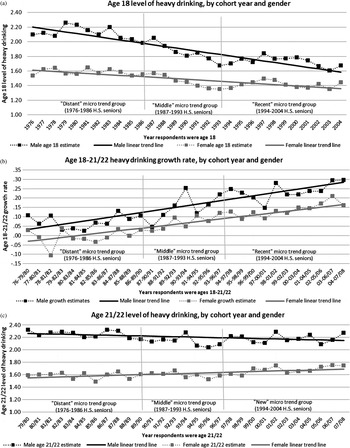
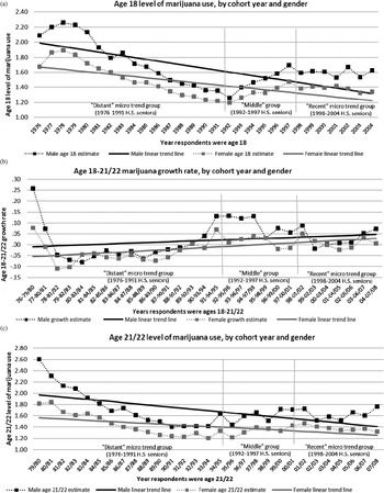
Finally, by including cohort year as a grouping variable in the baseline age 18–21/22 growth model, we estimated the age 18 level of use and the age 18–21/22 growth rate for each of the 29 individual cohort years. By doing the same when estimating the mean level at age 21/22, we estimated the age 21/22 level of use for each of the cohort years as well. For both heavy drinking (Figure 2) and marijuana use (Figure 3), each of these estimates (i.e., age 18 level, age 18–21/22 growth rate, age 21/22 level) is plotted by cohort year to provide a visual indication of macro and microtrends in each.
Historical trends in heavy drinking (last 2 weeks) by cohort year and gender.

Historical trends in marijuana use (last 30 days) by cohort year and gender.

Aim 1: Magnitude and scope of historical variation of young adult drug use
Macrotrends in drug use
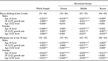
To examine macrotrends in the age 18 level and the age 18–21/22 growth rate, we built on the baseline growth model in Figure 1 and included the variable cohort year as an exogenous predictor of each drug use factor (cohort year age 18–21/22 growth model; Figure 1). The result is an estimate of the linear change in each drug use growth factor (the age 18 intercept and the age 18–21/22 growth rate) for each annual increase in cohort year. Likewise, to examine macrotrends in the age 21/22 level, in a separate model we included cohort year as an exogenous predictor of age 21/22 use (i.e., a path model with cohort year predicting age 21/22 use; hereafter, we refer to this model as the cohort year age 21/22 path model). Results are presented in the first column of Table 3. Because this analytical approach is analogous to fitting a regression, or linear-trend, line through the estimate plots in Figures 2 and 3, the figures include these linear-trend lines as well. Since our first aim is descriptive, no control variables are included.
Cohort year predicting young adult drug use, the whole sample, and by microtrend groups

Note: Estimates sharing same superscript letter differ significantly from one another. Model comparison results (listed below) and pairwise comparisons among the microtrend groups are matched by superscript letter. All estimates are unstandardized path (regression) coefficients.
aΔχ2 (1) = 13.83, p < .01. bΔχ2 (1) = 21.27, p < .01. cΔχ2 (1) = 7.30, p < .01. dΔχ2 (1) = 5.58, p < .05. eΔχ2 (1) = 23.60, p < .01. fΔχ2 (1) = 25.97, p < .01. gΔχ2 (1) = 5.65, p < .05. hΔχ2 (1) = 6.65, p < .01. iΔχ2 (1) = 205.62, p < .01. jΔχ2 (1) = 50.96, p < .01. kΔχ2 (1) = 30.33, p < .01. lΔχ2 (1) = 4.88, p < .05. mΔχ2 (1) = 3.87, p < .05. nΔχ2 (1) = 49.58, p < .01. oΔχ2 (1) = 22.93, p < .01. pΔχ2 (1) = 182.22, p < .01. qΔχ2 (1) = 28.25, p < .01. rΔχ2 (1) = 49.82, p < .01. sΔχ2 (1) = 68.42, p < .01. tΔχ2 (1) = 23.35, p < .01. *p < .05. **p < .01.
As expected, the relation between cohort year and the age 18 level of heavy drinking was negative for both males (–0.022) and females (–0.009), indicating that level declined across cohort year. In addition, the relation between cohort year and the age 18–21/22 growth rate in heavy drinking was positive for both males (0.009) and females (0.007), indicating that growth rate increased across cohort year. Thus, historical trends in the age 18 level and the age 18–21/22 growth rate moved in opposite directions. To illustrate this phenomenon empirically, we correlated at the cohort level (i.e., individuals nested within cohort) the age 18 intercept and the age 18–21/22 growth rate. The correlation for both males (r = –.93, p < .001) and females (r = –.86, p < .001) was negative, indicating that the lower a given cohort's age 18 intercept, the higher its age 18–21/22 growth rate. For males, the historical declines in the age 18 level of heavy drinking narrowly outpaced the historical increases in the age 18–21/22 growth rate, as evidenced by the modest negative relation between the age 21/22 heavy drinking level and cohort year (–0.004). However, for females the level of age 21/22 use increased across cohort year (0.005), indicating that the historical increases in the age 18–21/22 growth rate outpaced the historical declines in the age 18 level.
As with heavy drinking, for marijuana the relation between cohort year and the age 18 level was negative for both males (–0.024) and females (–0.016), the relation between cohort year and the age 18–21/22 growth rate was positive for both males (0.002) and females (0.003), and at the cohort level these trends were inversely related (males: r = –.49, p < .001; females: r = –.51, p < .001). Compared to heavy drinking, historical increases in the age 18–21/22 marijuana use growth rate were modest. Due to the modest increases in growth rate, the sharp historical declines in the age 18 level easily outpaced the historical increases in the age 18–21/22 growth rate for both genders, as evidenced by the still sizable negative relation between marijuana use level at age 21/22 and cohort year for both males (–0.020) and females (–0.011).
Microtrends in drug use
Building on the cohort year age 18–21/22 growth model and the cohort year age 21/22 path model, we examined microtrends in heavy drinking and marijuana use by adding their respective microtrend groups (i.e., distant, middle, and recent) as a grouping variable and performing multiple-group analyses. Doing so allowed us to examine whether the relation between cohort year and drug use (i.e., age 18 level, age 18–21/22 growth rate, and age 21/22 level) varied across microtrend group. Results are presented separately for each microtrend group in columns 2 through 4 of Table 3.
Although the age 18 level of heavy drinking decreased most sharply among the 87–93 group for both genders (males = –0.057, females = –0.035), the age 18–21/22 growth rate also increased most sharply among the 87–93 group (males = 0.021, females = 0.013). For males, these microtrends in the age 18 level and the age 18–21/22 growth rate effectively canceled each other out, rendering the level of age 21/22 heavy drinking invariant across the three microtrend groups. For females, the level of age 21/22 heavy drinking varied across the microtrend groups and historical increases were limited to the 94–04 group (0.010). For marijuana use, microtrends in the age 18 level were both pronounced and irregular for both genders: the level of use at age 18 decreased sharply across cohort year among the 76–91 group (males = –0.070, females = –0.047), but then the pattern reversed among the 92–97 group, whose level of use increased sharply across cohort year (males = 0.076, females = 0.049). Among the 98–04 group, the age 18 level no longer increased across cohort year for either gender: for males (0.002) use was stable, and for females (–0.013) use decreased modestly. Unlike the age 18 level of use, microtrends in the age 18–21/22 growth rate were muted. For males, the age 18–21/22 growth rate varied across cohort year only among the 87–93 group (–0.017), and for females, the relation between cohort year and the age 18–21/22 growth rate was invariant across the three microtrend groups. Regarding the age 18–21/22 growth rate, it may seem strange that the macrotrend for males increased modestly across cohort year (0.002) while the three microtrends were all either stable or decreasing across cohort year. The extreme outliers at the earliest portion of the 76–91 microtrend group (see Figure 3b) appear to have had a disproportionate influence on that microtrend group's estimate, rendering its relation between cohort year and the age 18–21/22 growth rate nonsignificant even though the growth rate typically increased from one cohort year to the next between 1976 and 1991. Finally, because microtrends in the age 18–21/22 marijuana growth rate were muted, for both genders microtrends in the age 21/22 level closely tracked microtrends in the age 18 level.
To summarize, as was the case for macrotrends, microtrends in the age 18–21/22 growth rate tended to move in the opposite direction of microtrends in the age 18 level; the more the age 18 level declined, the more the age 18–21/22 growth rate steepened upward in that particular microtrend group and vice versa. As a result of this inverse pattern, microtrends in the age 21/22 level were muted relative to microtrends in both the age 18 level and the age 18–21/22 growth rate. This was especially the case for heavy drinking. Finally, for both heavy drinking and marijuana use, historical fluctuations in the age 18 level, the age 18–21/22 growth rate, and the age 21/22 level were relatively muted among the most recent microtrend groups (the recent modest increases in the female heavy drinking age 18–21/22 growth rate and the age 21/22 level were important exceptions).
Aim 2: Possible mechanisms of acceleration in growth of young adult drug use
Historical changes in the distribution of social roles
To this point, all analyses have used a sample weight that adjusts for MTF's oversampling of drug users. Building on this sample weight, we created a distribution weight that renders the Wave 2 (ages 19–20) distribution of young adult social roles (i.e., rates of college attendance, marriage, and parenthood) among each of the 1977–2004 cohorts to be equal to the distribution among the 1976 cohort. We did so by using inverse-probability weighting (Curtis, Hammill, Eisenstein, Kramer, & Anstrom, Reference Curtis, Hammill, Eisenstein, Kramer and Anstrom2007; Jager, Reference Jager2011), a technique used commonly in clinical and epidemiological research that adjusts the distribution of key demographic variables in one or more samples to match the distribution of a target sample. Here we matched the distribution of college status, marital status, and parental status among the 1977 cohort to the distribution of our target 1976 cohort separately for each gender. In sequence, we then did the same for the 1978–2004 cohorts. Confirming that the distribution weight functioned as intended, rates of college status, marital status, and parental status were equivalent (to the nearest tenth of a percent) across all 29 cohorts after applying the weight. In addition, the sample size of the overall sample (N = 38,926) and of each cohort year matched those obtained when applying the original sample weight. Thus, this distribution weight adjusts for both the oversampling of drug users and cohort differences in the distribution of social roles.
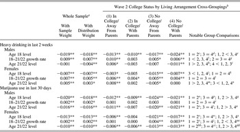
Using the cohort year age 18–21/22 growth model and the cohort year age 21/22 path model, we carried out two sets of analyses: one incorporating the original sample weight (results listed in the first column of Table 4) and a second incorporating the distribution sample weight (results listed in the second column of Table 4). Because the second set of analyses removes cohort differences in the distribution of social roles as a potential confound, comparing the results from these two sets of analyses allows us to assess the extent to which historical variation in young adult drug use is explained by historical variation in the distribution of social roles. Both sets of analyses include controls for minimum legal drinking age, race (effect coded with White = 1 and other = –1), and instability in marital, parental, and college status between Waves 2 and 3. Aside from the male historical trend in age 21/22 level of heavy drinking switching from flat to negative, estimates were similar across both sets of analyses, indicating that macrotrends in the relation between cohort year and drug use were largely independent of historical variation in the distribution of young adult social roles. Microtrends in drug use (as described in the previous section) were equally evident when applying the distribution weight (results not tabled). These findings indicate that microtrends in drug use were also independent of historical variation in the distribution of young adult social roles.
Cohort year predicting young adult drug use, with and without social role distribution weight and by Wave 2 college status and living arrangements

Note: Model comparison results (listed below) and notable group comparisons (listed in last table column) are matched by superscript letter. All estimates are unstandardized path (regression) coefficients.
aControls for minimum legal drinking age, race, and changes in marital status, parental status, and college status across Wave 2 and Wave 3.
bControls for minimum legal drinking age, race, Wave 2 and 3 marital status and parental status, and instability in college status and living arrangements.
cΔχ2 (1) = 0.43, p = 0.52. dΔχ2 (1) = 3.20, p = 0.08. eΔχ2 (1) = 15.48, p < 0.01. fΔχ2 (1) = 5.46, p < 0.05. gΔχ2 (2) = 0.94, p = .63. hΔχ2 (1) = 16.30, p < .01. iΔχ2 (1) = 12.55, p < .01. jΔχ2 (1) = 14.10, p < .01. kΔχ2 (2) = 3.84, p = .15. lΔχ2 (3) = 3.05, p = .38. mΔχ2 (1) = 13.70, p < .01. nΔχ2 (1) = 7.79, p < .01. oΔχ2 (1) = 0.55, p = .46. pΔχ2 (1) = 0.40, p = .53. qΔχ2 (1) = 14.38, p < .01. rΔχ2 (3) = 0.78, p = .86. sΔχ2 (1) = 0.52, p = .47. tΔχ2 (1) = 0.04, p = .84. uΔχ2 (1) = 9.04, p < .01. vΔχ2 (1) = 0.64, p = .43. wΔχ2 (1) = 1.70, p = .19. xΔχ2 (1) = 40.84, p < .01. yΔχ2 (1) = 0.44, p = .51. zΔχ2 (1) = 0.53, p = .47. aaΔχ2 (1) = 5.76, p < .05. bbΔχ2 (1) = 0.01, p = 97. ccΔχ2 (1) = 0.01, p = .99. ddΔχ2 (1) = 6.96, p < .01.
*p < .05. **p < .01.
College status and living arrangements as moderators
Building again on the cohort year age 18–21/22 growth model and the cohort year age 21/22 path model, we conducted multiple-group analyses using the four college status by living arrangement groups (as measured at Wave 2) as the grouping variable. We used the original sample weight and included the following as controls: minimum legal drinking age, race (effect coded), Waves 2 and 3 marital status (effect coded), Waves 2 and 3 parental status (effect coded), and Waves 2 and 3 instability in college status and living arrangements. Group estimates are presented in columns 3 through 6 of Table 4; notable group comparisons are presented in the last column.
Overall, when college status and living arrangements moderated historical variation in level and growth rate of heavy drinking, heavy drinking across cohort year tended to either increase at a faster pace or decrease at a slower pace among those in college, and at times specifically among those both in college and living away from their parents. For example, for males decreases across cohort year in the age 18 level were more pronounced among those not in college, regardless of living arrangements (–0.017, –0.024), while for females decreases were more pronounced among those both not in college and living away from parents (–0.015). In addition, though for females increases in the age 18–21/22 growth rate across cohort year did not vary across the four subgroups, for males increases in the age 18–21/22 growth rate across cohort year were the highest among those both in college and living away from parents (0.010). Finally, for males decreases in the age 21/22 level across cohort year were only evident among those both not in college and living with their parents (–0.011); the age 21/22 level of heavy drinking actually increased across cohort year among those both in college and living away from their parents (0.006). For females decreases in the age 21/22 level across cohort year were only evident among those both not in college and living away from their parents (–0.005); the age 21/22 level of heavy drinking increased across cohort year among those both in college and living away from their parents (0.008).
In general, historical decreases in the age 18 and the age 21/22 levels of marijuana use were generally more pronounced among those not in college. For example, for both genders decreases across cohort year in the age 18 level were higher among those not in college, regardless of living arrangements (males = –0.054, –0.021; female = –0.021, –0.017). Though increases across cohort year in the age 18–21/22 marijuana growth rate did not vary across the four male subgroups, for females increases were only evident among those not in college (0.004, 0.003). Finally, for both genders the age 21/22 level of marijuana use decreased at a faster pace among those not in college, regardless of living arrangements (males = –0.020, –0.021; females = –0.013, –0.013). For females, though the age 21/22 level decreased at a faster pace among those not in college, the difference across college status in the rate of decrease in level of use across cohort year was smaller at age 21/22 than at age 18.
Population microtrends in drug use were equally evident within each of the four college status by living arrangement subgroups. These findings indicate that microtrends in drug use were not moderated by college status and living arrangements (not tabled).
Discussion
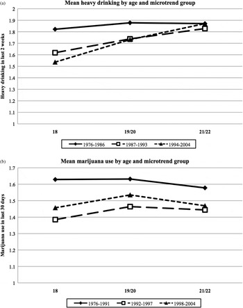
Over the last three decades, the developmental course of drug use across the initial young adult years, from age 18 to 22, has changed in two important ways. First, levels of alcohol and marijuana use declined (cohort effect). For marijuana, historical decreases in levels of use were slightly larger at the younger end of the age band (modest cohort by age interaction). Figure 4b, which lists the marijuana use means by age and microtrend group, illustrates this point. Historical declines in the levels of heavy drinking were only evident at the younger end of the age band (strong cohort by age interaction); levels of heavy drinking among 21- to 22-year-olds were relatively stable historically, as illustrated in Figure 4a. Second, underlying these cohort by age effects, young adult trajectories of marijuana use and heavy drinking have steepened upward across the last three decades, especially in the case of heavy drinking. Both historical declines in levels of use and historical increases in growth of use were most evident during the mid-1980s and early 1990s. Generally, historical variation in levels and growth of drug use was unrelated to changes in the distribution of social roles and in young adult contexts (college status and living arrangements). Exceptions are discussed below.
Drug use means by age and microtrend group.

Macro- and microtrends in young adult drug use
Across the last three decades, the young adult heavy drinking growth rate increased threefold for males (from 0.10 among the 1976 cohort to 0.30 among the 2004 cohort) and sixfold for females (from 0.03 among the 1976 cohort to 0.17 among the 2004 cohort). These sharp increases in growth rates offset the declines in age 18 levels such that the age 21/22 level of heavy drinking remained relatively stable (the 1994–2004 female cohorts were the exception, among whom the level of age 21/22 heavy drinking increased modestly across cohorts). Findings regarding historical variation in the age 18 levels of heavy drinking are not new (Johnston et al., 2009a) but are placed in a broader context by this study's focus on cohort differences in the young adult heavy drinking growth rate. While different cohorts are known to have different starting points (i.e., at age 18 they engage in different amounts of heavy drinking), this study shows that, by and large, they have a similar end point (i.e., at age 21/22 they engage in similar amounts of heavy drinking). Although typically applied to intracohort differences, in developmental science this phenomenon is termed equifinality (Bertalanffy, Reference Bertalanffy1968), which is multiple pathways to the same or similar end point (Cicchetti & Rogosch, Reference Cicchetti and Rogosch2002; Schulenberg & Zarrett, Reference Schulenberg, Zarrett, Arnett and Tanner2006). While the overall decline in age 18 heavy drinking is clearly a trend welcomed by public health officials and policymakers, the acceleration in the rate of increase points to unique intervention challenges (Hingson, Heeren, Winter, & Wechsler, Reference Hingson, Heeren, Winter and Wechsler2005). Any increase in heavy drinking from age 18 to 21/22 increases the risk of negative consequences (Carter, Brandon, & Goldman, Reference Carter, Brandon and Goldman2010; Chassin, Hussong, & Beltran, Reference Chassin, Hussong, Beltran, Lerner and Steinberg2009; Schulenberg, O'Malley, Bachman, Wadsworth, & Johnson, Reference Schulenberg, O'Malley, Bachman, Wadsworth and Johnston1996); it is likely that the faster the increase, the less experience one has with heavy drinking situations and the more risk is involved (Schulenberg & Maggs, Reference Schulenberg and Maggs2002).
Historical declines in adolescent marijuana use were not as fleeting; sharp declines in adolescent marijuana use greatly outpaced the modest increase in young adult growth rates. Due to this pattern, historical trends in the age 21/22 levels closely tracked historical trends in adolescent levels, which were extremely irregular (Johnston et al., Reference Johnston, O'Malley, Bachman and Schulenberg2010a, Reference Johnston, O'Malley, Bachman and Schulenberg2010b). Focusing on age 18 marijuana use among the 1984–1997 cohorts of high school seniors, Bachman, Johnston, and O'Malley (Reference Bachman, Johnston and O'Malley1999) found that historical fluctuations in use were inversely related to historical fluctuations in the perceived risks of marijuana use. Given our finding that intercohort differences in the level of marijuana use are largely stable across the ages of 18 and 21/22 (modest cohort by age effect), intercohort differences in the perceived risks of marijuana use may be stable across these ages as well.
Steepening upward growth: Just a “rebound” from adolescence?
The fact that a greater proportion of today's young adults are in college and unmarried was, by and large, unrelated to historical variation in level and growth of young adult drug use. The exception was the age 21/22 level of heavy drinking among males, which was stable before adjusting for historical variation in young adult rates of college attendance, marriage, and parenthood, but decreased slightly after taking these adjustments into account. In addition, cohort differences in young adult drug use growth were generally not larger within social roles associated with increased opportunity for exploration and experimentation, such as going to college and living away from home. The exception was heavy drinking growth among males in college and living way from parents, which accelerated the fastest. Finally, though historical decreases in the age 21/22 levels were smaller among those who attended college, in most of these cases adolescent (i.e., age 18) decreases were also smaller among those who attended college. This pattern suggests that historical variation in the age 21/22 levels of drug use is not predicted by college status but by adolescent factors that differentiate adolescents who go on to attend college from those who do not. Factors known to predict college attendance include parental income and education, and prior academic success (Alexander, Holupka, & Pallas, Reference Alexander, Holupka and Pallas1987; Bachman et al., Reference Bachman, O'Malley, Schulenberg, Johnston, Freedman-Doan and Messersmith2008).
Fluctuations in young adult growth were strongly and inversely associated with fluctuations in adolescent (age 18) use. Thus, the more a given cohort's adolescent drug use deviated from the across-cohort average, the more quickly that cohort's drug use “rebounded” in the other direction across young adulthood. Collectively, our findings suggest that historical variation in young adult drug use growth is less related to young adult proximal factors and more related (albeit negatively) to adolescent distal factors. A possible explanation for this pattern of findings is that the influence of whatever was responsible for the historical fluctuations in adolescent use diminished as individuals aged through young adulthood. Research has linked historical variation in adolescent drug use to historical fluctuations in attitudes and beliefs about both licit and illicit drug use (Bachman et al., Reference Bachman, Johnston and O'Malley1990, Reference Bachman, Johnston and O'Malley1999, Reference Bachman, O'Malley, Schulenberg, Johnston, Bryant and Merline2001; Johnston et al., Reference Johnston, O'Malley, Bachman and Schulenberg2010a; Keyes et al., in press). Such attitudes and beliefs have in turn been linked to historical fluctuations in antidrug media campaigns, federal antidrug initiatives, and drug use laws (Hingson, Heeren, & Winter, Reference Hingson, Heeren and Winter1994; Hingston et al., 2005; Johnston et al., Reference Johnston, O'Malley, Bachman and Schulenberg2010a). Because these antidrug efforts have been primarily aimed at youth and are school based, their influence may diminish as individuals age through young adulthood.
In contrast to marijuana use, young adult growth in heavy drinking rebounded sharply, often equaling, if not outpacing, historical declines in adolescent heavy drinking. The strong rebound in heavy drinking, relative to marijuana use, might be explained by the fact that, aside from efforts to reduce drunk driving, many prevention efforts focus on underage drinking (opposed to “of-age” drinking) and may become obsolete as individuals age into legal drinking. This is not the case for antimarijuana messaging, which is not age specific because marijuana use is illegal at any age. Consistent with this pattern, we found across all cohorts that the positive association between a higher minimum legal drinking age and a higher young adult growth rate was much stronger for heavy drinking than for marijuana use. In addition, the stronger rebound for heavy drinking may also be explained by the substantial countermessaging within media advertising and cultural norms that encourage alcohol consumption among those of legal age; there is no such countermessaging for marijuana use.
The chronosystem and historical variation in young adult drug use
According to Bronfenbrenner's ecological model of human development (Reference Bronfenbrenner1977, Reference Bronfenbrenner1994), the chronosystem is the most distal context within one's ecology and encompasses sociohistorical variation in societal-level factors, such as opportunity structures and life-course options. More distal contexts influence the individual indirectly through their effects on more proximal contexts. Though we did not examine the chronosystem directly, we did examine how historical changes in more proximal contexts (i.e., college status and living arrangements) relate to historical variation in young adult growth rates of drug use. Regarding these more proximal contexts, we focused on historical changes in their distribution and the opportunities for exploration and experimentation that they provide. Both of these historical changes are thought to be manifestations of historical variation in more distal, societal factors (i.e., the chronosystem), namely, historical changes in social structure (Arnett, Reference Arnett2000; Shanahan, Reference Shanahan2000). Likewise, historical fluctuation in societal factors thought to contribute to the adolescent drug use trends discussed above (i.e., society's attitudes and beliefs as well as public policy regarding drug use and antidrug efforts aimed at youth) are all encompassed within the chronosystem. Although our examination indicated that the historical changes in young adult drug use were largely unrelated to historical variation in the proximal contexts of young adults, future research should examine more directly the role of historical variation in more distal, societal factors.
The ecological–developmental model of child maltreatment (Belsky, Reference Belsky1980, Reference Belsky1993; Cicchetti & Lynch, Reference Cicchetti and Lynch1993) may provide a useful theoretical framework for doing so. The model views maladjustment as the product of transactions among forces within the individual and the ecological contexts. Though individuals play an active role in their own development, they are also influenced by the immediate contexts surrounding them, and those contexts are, in turn, influenced by more distal society-level factors. Thus, historical variation in young adult drug use likely entails layered interactions between bottom-up and top-down factors that, when taken as a whole, help explain ongoing chronosystem effects.
Strengths and limitations
Several important strengths of this study derive from the use of consistent measures in national multicohort panel data spanning the transition to adulthood. We offer a view of drug use as a moving target developmentally and historically that is typically unavailable in longitudinal data sets with one or few cohorts. In addition, our emphasis on heavy drinking and marijuana use showed that historical trends in both level and growth vary dramatically depending upon whether the drug of focus is licit or illicit.
This study also has several important limitations. First, our examination of microtrends in growth rates is based on known microtrends in level of use. In the absence of past research documenting historical variation in growth, this study's choice of period bands for microtrends in level of use may not be the ideal period bands for microtrends in growth rates. Second, our findings may generalize less to those of lower socioeconomic status and those who report elevated senior year drug use because their rates of attrition were slightly higher. Third, because our examination of college status focused on those attending a 4-year college full time, the extent to which our findings generalize to other types of college students is unclear. Fourth, because our examination was limited to three time points, we could model only linear growth. However, looking at Figure 4, it appears that drug use growth followed a negative quadratic trend (i.e., rate of increase declined over time), and this was especially true for marijuana use. Nonetheless, because preliminary analyses indicated that quadratic trends in drug use growth were equivalent across cohorts, our inability to model quadratic trends did not obscure our examination of cohort differences in growth or level. Fifth, because we controlled for instability in social roles and living arrangements, it is unclear how our findings generalize to the minority of transitioning adults whose social roles and living arrangements are characterized by instability.
Conclusions and implications
By focusing on intercohort differences in trajectories, our study builds on important cross-sectional analyses of levels of drug use that collectively point to a decline in drug use among young adults across the last three decades (Grucza et al., Reference Grucza, Bucholz, Rice and Bierut2008; Johnston et al., Reference Johnston, O'Malley, Bachman and Schulenberg2010a, Reference Johnston, O'Malley, Bachman and Schulenberg2010b; Kerr et al., Reference Kerr, Greenfield, Bond, Ye and Rehm2009). In the case of marijuana use, these studies offered findings consistent with ours. In the case of heavy drinking, their findings were partially consistent with ours. While the level of adolescent heavy drinking has declined considerably across the last three decades, heavy drinking among 21- to 22-year-olds has not, owing to a sharp increase in the young adult growth rate. Findings suggest that antidrug efforts directed at youth and aimed at curbing underage drinking and illicit drug use have been successful. However, an unintended side effect of these efforts appears to be an accelerated increase in young adult heavy drinking, posing risks for both short- and long-term adjustment.