2. Preliminaries and notation

Consider a multitype Galton–Watson process with countably infinite type set $\mathcal{X}_d= \{ \langle k,i \rangle \,:\, k \geq 0, \, 1 \leq i \leq d \}$ for some $ 1 \leq d < \infty$ . It will be implicitly assumed that the types in any subset $A\subseteq\mathcal{X}_d$ are ordered lexicographically. We assume that the process initially contains a single individual whose type is denoted by $\varphi_0$ . It then evolves according to the following rules:

1. (i) each individual lives for a single generation, and

2. (ii) at death gives birth to $\textbf{\textit{r}}=(r_{ \ell})_{{ \ell} \in \mathcal{X}_d}$ offspring, that is, $r_{\langle 0,1 \rangle }$ individuals of type $\langle 0,1 \rangle$ , $r_{\langle 0,2 \rangle}$ individuals of type $\langle 0,2 \rangle$ , etc., where the vector $\textbf{\textit{r}}$ is chosen independently of all other individuals according to a probability distribution, $p_j( \cdot\!)$ , specific to the parental type $j \in \mathcal{X}_d$ .

We say that a type- $\langle k,i \rangle$ individual is in level k and phase i. We partition $\mathcal{X}_d$ in two ways: by level, $\mathcal{X}_d={\bigcup}_{k \geq 0} L_k$ , where $L_k= \{ \langle k,1 \rangle ,\langle k,2 \rangle , \dots, \langle k,d \rangle \}$ ; and by phase, $\mathcal{X}_d=\bigcup_{i=1}^d A_i$ , where $A_i = \{ \langle 0,i \rangle , \langle 1,i \rangle , \dots \}$ . The primary assumption we make is that an individual in level k cannot have any level $j > k+1$ offspring. In other words, the offspring vector from a level-k individual belongs to the set

\begin{equation*}R_{k,d} \,:\!= \left\{ \textbf{\textit{r}} \in {\mathbb N}_0^{\mathcal{X}_d}\,:\, \, r_{j}=0 \text{ for all } j \in \bigcup^\infty_{i=k+2} L_i \right\}.\end{equation*}

While this assumption is made throughout, many of our results hold without it. We refer to the resulting process as a block lower Hessenberg branching process, or block LHBP for short.

The branching process is defined on the Ulam–Harris space [Reference Harris10, Chapter VI], labelled $( \Omega, \mathcal{F}, \mathbb{P})$ , as follows. Let $\mathcal{J} = \bigcup_{n \geq 0} \mathcal{J}_n$ , where $\mathcal{J}_n$ describes the virtual nth generation. That is, $\mathcal{J}_0= \mathcal{X}_d$ , where $\varphi_0 \in \mathcal{J}_0$ specifies the type of the root, and, for $n\geq 1$ , $\mathcal{J}_n={ \mathcal{X}_d \times} ( {\mathbb N} \times \mathcal{X}_d \times {\mathbb N})^n$ , where $(\varphi_0;\,i_1, j_1, y_1;\, \dots;\, i_n, j_n, y_n)$ denotes the $i_n$ th child of type $j_n$ born to $(\varphi_0;\, i_1, j_1, y_1;\, \dots;\, i_{n-1}, j_{n-1}, y_{n-1})$ , and $y_n$ denotes the individual’s unique identification number (to define the process on the Ulam–Harris space we do not generally require the identification number $y_n$ ; however, this additional index will be used in the following, see Remark 3.1). Each virtual individual $I \in \mathcal{J}$ is assigned a random offspring vector ${\textbf{\textit{N}}}(I) =({N}_{\ell}(I))_{{ \ell} \in \mathcal{X}_d}$ that takes values in $R_{k,d}$ when I’s type belongs to level k, and has distribution ${p}_j(\!\cdot\!)$ when I is of type j, independently of all other individuals. The random set of individuals who appear in the population, $X = \bigcup_{n \geq 0} X_n$ , is then defined recursively from the values of ${\textbf{\textit{N}}}(I)$ as follows:

\begin{equation*}X_0 = \{ \varphi_0 \}, \qquad X_n = \{ x = ( \tilde{x};\, i_n, j_n, n) \in \mathcal{J}_n \,:\, \tilde{x} \in X_{n-1}, \, i_n \leq N_{j_n}(\tilde{x}) \}.\end{equation*}

The population in generation n is described by the vector $\textbf{\textit{Z}}_n$ with entries

\begin{equation*}Z_{n,j} = \sum_{I \in \mathcal{J}_n } \mathrm{1} ( I \in X_n , \, \, j_n = j ), \qquad j \in \mathcal{X}_d.\end{equation*}

We will often refer to branching processes by their sequence of population vectors $\{ \textbf{\textit{Z}}_n \}_{n \geq 0}$ .

From the set of probability distributions $\{ p_j (\!\cdot\!) \}_{j\in\mathcal{X}_d}$ we define the probability-generating function ${\textbf{\textit{G}}}(\!\cdot\!) \,:\, [0,1]^{\mathcal{X}_d} \to [0,1]^{\mathcal{X}_d}$ , which contains entries

(1) \begin{equation}G_j ( \textbf{\textit{s}} ) = \sum_{ \textbf{\textit{r}} } p_{j}(\textbf{\textit{r}}) \textbf{\textit{s}}^{\textbf{\textit{r}}} = \sum_{ \textbf{\textit{r}} } p_{j}(\textbf{\textit{r}}) \prod_{ k\in\mathcal{X}_d } s_k^{r_k},\qquad j\in\mathcal{X}_d.\end{equation}

We denote the n-fold composition of ${\textbf{\textit{G}}}(\!\cdot\!)$ by ${\textbf{\textit{G}}}^{(n)}(\!\cdot\!)$ . For any $n \geq 0$ and any set of types $A \subseteq \mathcal{X}_d$ , let

\begin{equation*}{\mathcal{E}}_n(A) = \left\{ \omega \in \Omega\,:\, \sum^\infty_{\ell=n} \sum_{i \in A} Z_{\ell,i} =0 \right\}\end{equation*}

denote the event that no individual of type $i \in A $ appears in the population from generation n, and let $\mathcal{E}(A)= \lim_{n \to \infty} \mathcal{E}_n(A)$ represent the event of eventual extinction in A. For $n\geq 0$ , we define the vector $\textbf{\textit{q}}_n{(A)}$ whose ith element is given by $q_{n,i}(A) = \mathbb{P}_i ( \mathcal{E}_n(A) )$ , where $\mathbb{P}_i(\!\cdot\!)\,:\!=\break \mathbb{P}(\cdot \mid \varphi_0=i)$ . The vector $\textbf{\textit{q}}_0{(A)}$ , which represents the probability that no individual with type in A will ever be produced, plays an important role in the following. The vectors $\{ \textbf{\textit{q}}_n(A)\}_{n \geq 0}$ form a monotone nondecreasing sequence that satisfies the equation

\begin{equation*}\textbf{\textit{q}}_{n+1}(A) = {\textbf{\textit{G}}}(\textbf{\textit{q}}_n(A)),\qquad n\geq 0.\end{equation*}

Consequently, by the monotone convergence theorem, each extinction probability vector $\textbf{\textit{q}}(A)\,:\!= (\mathbb{P}_i(\mathcal{E}(A)))_{i \in \mathcal{X}}$ is obtained as the limit of the sequence $\{ \textbf{\textit{q}}_n(A)\}$ as $n \to \infty$ . In addition, by continuity of ${\textbf{\textit{G}}}({\cdot})$ , we have

(2) \begin{equation}\textbf{\textit{q}}(A)={\textbf{\textit{G}}}( \textbf{\textit{q}}(A)),\end{equation}

which implies that $\textbf{\textit{q}}(A)$ is an element of the set $S = \{ \textbf{\textit{s}} \in [0,1]^{\mathcal{X}_d} \,:\, \textbf{\textit{s}} = {\textbf{\textit{G}}}(\textbf{\textit{s}}) \}$ . Let $T_k = \bigcup^k_{i=0} L_i$ be the set of types whose level is at most k. Following [Reference Hautphenne, Latouche and Nguyen11] we refer to $\bigcap_{k=1}^\infty \mathcal{E}(T_k )$ and $\mathcal{E}(\mathcal{X}_d)$ as the partial and global extinction events, respectively, and denote their corresponding extinction probability vectors by ${\tilde{\textbf{\textit{q}}}}$ and $\textbf{\textit{q}}$ .

The mean progeny matrix M is an infinite matrix whose entries are given by

\begin{equation*}M(i,j) = \left. \frac{\partial G_i ( \textbf{\textit{s}} )}{\partial s_j } \right|_{\textbf{\textit{s}}= \textbf{1}}, \qquad \text{ for } i,j \in \mathcal{X}_d,\end{equation*}

where M(i, j) can be interpreted as the expected number of type-j children born to a parent of type i. By assumption M has a block lower Hessenberg structure,

\begin{equation*}M=\left[\begin{array}{c@{\quad}c@{\quad}c@{\quad}c@{\quad}c@{\quad}c}M_{00} & M_{01} & 0 & 0 & 0& \dots \\[3pt] M_{10} & M_{11} & M_{12} & 0 & 0 & \\[3pt] M_{20} & M_{21} & M_{22} & M_{23} & 0 & \\[3pt] M_{30} & M_{31} & M_{32} & M_{33} & M_{34} & \\[3pt] \vdots & & & & & \ddots\end{array}\right] \end{equation*}

where, for $k,l\geq 0$ , $M_{kl}\,:\!=(M(i,j))_{i\in L_k, j\in L_l}$ are square matrices of order d. We associate with M a weighted directed graph, referred to as the mean progeny representation graph. This graph has vertex set $\mathcal{X}_d$ and contains an edge from i to j of weight M(i, j) if and only if $M(i,j)>0$ . The branching process is said to be irreducible if there is a path between any two vertices in the mean progeny representation graph on $\mathcal{X}_d$ . It is well known (see for instance [Reference Hautphenne, Latouche and Nguyen11, Proposition 4.1) that

\begin{equation*}\nu(M) \leq 1 \quad \Leftrightarrow \quad {\tilde{\textbf{\textit{q}}}}=\textbf{1},\end{equation*}

where $\nu(M)\,:\!=\sup_{i,j}\big\{\limsup_n(M^n)_{ij}^{1/n}\big\}$ denotes the convergence norm of M.

For any $A \subseteq \mathcal{X}_d$ we define a branching process labelled $\{ {\tilde{\textbf{\textit{Z}}}}_n^{(A)} \}_{n\geq 0}$ . This process, constructed on $( \Omega, \mathcal{F}, \mathbb{P})$ , is such that, for any $\omega \in \Omega$ ,

\begin{equation*}\tilde{\textbf{\textit{N}}}^{(A)}(\omega,I) =\begin{cases}{\textbf{\textit{N}}}(\omega,I), \quad & I \in A, \\[5pt] 0, \quad & I \notin A,\end{cases}\end{equation*}

where the notation $I \in A$ means that the type of individual I is in A. In other words, an outcome of $\{ {\tilde{\textbf{\textit{Z}}}}_n^{(A)} \}$ corresponds to one of $\{ \textbf{\textit{Z}}_n \}$ in which the individuals in $\bar{A}\,:\!=\mathcal{X}_d \backslash A$ are sterile, that is, they produce no offspring. The process $\{ {\tilde{\textbf{\textit{Z}}}}_n^{(A)} \}$ performs two roles that have parallels in the study of Markov chains on $\mathcal{X}_d$ . First, $\{ ({ \tilde Z}_{n,x}^{(A)})_{x \in A} \}_{n\geq 0}$ is the branching process formed by immediately killing offspring with type in $\bar{A}$ , that is, the process with the taboo subset $\bar{A}$ . Second, $(\tilde Z_{n,x}^{(T_k)})_{x \in L_{k+1}}$ is the vector counting the lines of descent that first enter level $k+1$ in generation n, that is, the vector of n-step first passage paths to $\bar{T}_k$ . We let $\tilde{M}^{(A)}= (M(i,j))_{ i,j \in A}$ be the mean progeny submatrix restricted to the types in A, and we denote by ${\tilde{\textbf{\textit{q}}}}^{(A)}$ the global extinction probability vector of $\{ {\tilde{\textbf{\textit{Z}}}}_n^{(A)} \}$ . In [Reference Braunsteins and Hautphenne7, Reference Hautphenne, Latouche and Nguyen11] the authors proved that ${\tilde{\textbf{\textit{q}}}}^{(T_k) }\to {\tilde{\textbf{\textit{q}}}}$ pointwise as $k \to \infty$ (where ${\tilde{\textbf{\textit{q}}}}^{(T_k) }$ was denoted as ${\tilde{\textbf{\textit{q}}}}^{(k) }$ ).

Throughout this paper we make repeated use of [Reference Bertacchi and Zucca1, Theorem 3.3] which, for completeness, we now state and prove.

Proof. We obtain (ii) $\Rightarrow$ (i) from the inequalities $\textbf{\textit{q}}(A) \geq \textbf{\textit{q}}_0(A)$ and $\textbf{\textit{q}}(A)\geq \textbf{\textit{q}}$ . The implication (i) $\Rightarrow$ (ii) follows from the monotonicity of ${\textbf{\textit{G}}}^{(n)}(\!\cdot\!)$ for all n : if $\textbf{\textit{q}}_0(A)\leq \textbf{\textit{q}}$ , then $\textbf{\textit{q}}_n(A)= {\textbf{\textit{G}}}^{(n)}(\textbf{\textit{q}}_0(A))\leq {\textbf{\textit{G}}}^{(n)}(\textbf{\textit{q}})=\textbf{\textit{q}}$ for all n, which implies ${\textbf{\textit{q}}(A)}\leq \textbf{\textit{q}}$ . The relations (ii) $\Rightarrow$ (iii) and (iii) $\Rightarrow$ (i) are immediate.

3. Partial and global extinction criteria

We begin our analysis by deriving partial and global extinction criteria for block LHBPs. These criteria extend the results in [Reference Braunsteins and Hautphenne7, Theorem 5.1]. They are based on the sequence of $d\times d$ matrices $\{\mathcal{M}_k\}_{k\geq 0}$ recursively defined as

(3) \begin{align}\mathcal{M}_k = {\sum_{n\geq 0} \left(M^{(k)}\right)^n\, M_{k,k+1}},\qquad k \geq 0,\end{align}

where

(4) \begin{equation}M^{(0)}=M_{00}, \qquad M^{(k)}\,:\!=\sum^{k}_{i=0} M_{ki}\,\mathcal{M}_{i\rightarrow k-1},\quad k\geq 1,\end{equation}

with $\mathcal{M}_{i\rightarrow j}\,:\!=\mathcal{M}_i\,\mathcal{M}_{i+1}\cdots\mathcal{M}_{j}$ for $i\leq j$ . We set $\mathcal{M}_k\,:\!= \infty$ if the series (3) does not converge, that is, if and only if ${\rm sp}({M}^{(k)})\geq 1,$ where sp $(\!\cdot\!)$ denotes the spectral radius. If the series converges, then $\mathcal{M}_k = {[I-M^{(k)}]^{-1}\, M_{k,k+1}}$ , and we can compute $\mathcal{M}_k$ recursively. We refer to the matrices $\mathcal{M}_k$ as step-up matrices because of their similarity to the step-down probability matrices $G^{(k)}$ in [Reference Latouche and Ramaswami14] defined for level-dependent quasi-birth-and-death processes. The term ‘step-up’ comes from the fact that, when $\mathcal{M}_j< \infty$ for $j = 1, \dots ,k$ , the matrix $\mathcal{M}_k$ records the expected number of first passage paths to $L_{k+1}$ that descend from a single individual in $L_k$ , or, more specifically,

\begin{equation*}\mathcal{M}_k(i,j) = \mathbb{E}_{\langle k,i \rangle} \Bigg( \sum_{n \geq 0} { \tilde Z}_{n,\langle k+1,j\rangle}^{(T_k)} \Bigg),\end{equation*}

where $\mathbb{E}_i(\!\cdot\!)\,:\!= \mathbb{E}(\!\cdot \mid \varphi_0=i)$ . We show this rigorously in Lemma 3.2. In addition to the step-up matrices $\{ \mathcal{M}_k \}$ , our global extinction criterion makes use of three regularity assumptions:

1. (A1) $\inf_{i} p_i (\textbf{0})>0$ .

2. (A2) $\inf_{k \geq 0, \, i,j \in \{ 1, \dots, d\} } p_{ \langle k,i\rangle }( 2 \textbf{\textit{e}}_{ \langle k,j\rangle})>0$ .

3. (A3) $\sup_{k \geq 0, \, i,j,l \in \{ 1, \dots, d\} } \mathcal{A}_k(i;\,j,l) < \infty$ , where the $d\times d^2$ matrices $\{\mathcal{A}_k\}$ satisfy the recursion

   \begin{align*} \mathcal{A}_0 & = \left[ I - M_{00} \right]^{-1} \left[V_{0,00} (\mathcal{M}_0\otimes \mathcal{M}_0)+V_{0,01} (\mathcal{M}_0\otimes I)+V_{0,10} (I\otimes \mathcal{M}_0)+V_{0,11}\right],\\ \mathcal{A}_k & = \left[ I - \sum^{k}_{i=0} M_{ki} \,\mathcal{M}_{i\rightarrow k-1} \right]^{-1}\cdot\left\{ \sum_{i=0}^{k+1} \sum_{j=0}^{k+1} V_{k,ij} \left(\mathcal{M}_{i\rightarrow k}\otimes \mathcal{M}_{j\rightarrow k}\right)\right.\\ & \qquad\qquad\qquad\left.+\sum_{i=0}^{k-1} M_{ki} \,\mathcal{M}_{i\rightarrow j-1}\, \mathcal{A}_j \left(\mathcal{M}_{j+1\rightarrow k}\otimes \mathcal{M}_{j+1\rightarrow k}\right)\right\},\qquad k\geq 1, \end{align*}
   the $d\times d^2$ matrices $V_{k,ij}$ have entries
   \begin{equation*} V_{k,ij}(a;\,b,c)\,:\!=\dfrac{\partial^2 G_{\langle k,a\rangle}(\textbf{\textit{s}})}{\partial s_{\langle i,b\rangle} \partial s_{\langle j,c\rangle}} \bigg|_{\textbf{\textit{s}}=\textbf{1}}, \end{equation*}
   and $\otimes$ denotes the Kronecker product.

Assumptions (A1) and (A2) are simple to verify in practice, whereas assumption (A3) is more challenging but can often be verified numerically. The matrices $\{\mathcal{M}_k\}$ and $\{\mathcal{A}_k\}$ have a physical interpretation, as we show in Lemma 3.2.

Theorem 2.1. If $\{\textbf{\textit{Z}}_n \}$ is irreducible, then

(5) \begin{equation}\mathcal{M}_k < \infty \mbox{ for all } k\geq 0 \quad\Leftrightarrow\quad \tilde{\textbf{\textit{q}}}=\textbf{1},\end{equation}

and if $\tilde{\textbf{\textit{q}}}=\textbf{1}$ , then under Assumptions (A1)–(A3),

(6) \begin{equation}\sum_{k=0}^\infty \left(\textbf{1}_d^\top\, \mathcal{M}_{0\rightarrow k} \, \textbf{1}_d \right)^{-1} = \infty \quad \Leftrightarrow \quad \textbf{\textit{q}}=\textbf{1},\end{equation}

where we recall that $\textbf{1}_d$ is a $d \times 1$ vector of ones.

Before turning to the proof of Theorem 2.1, we introduce the branching process $\{ \textbf{\textit{Y}}_k \}$ embedded within $\{ \textbf{\textit{Z}}_n \}$ , whose sample paths are constructed from those of $\{ \textbf{\textit{Z}}_n \}$ as follows: we define a function $f_g(\!\cdot\!) \,:\, \mathcal{J} \to \mathcal{J}$ that takes each line of descent $(\varphi_0;\, i_1, j_1, y_1;\, \dots;\, i_n, j_n, y_n)$ and deletes each triple $(i_k, j_k, y_k)$ whose level is not strictly larger than that of all its ancestors. 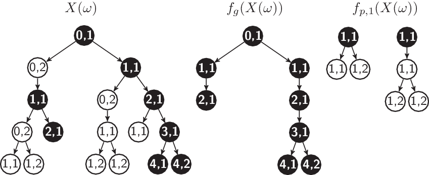For each $\omega \in \Omega$ the family tree of $\{\textbf{\textit{Y}}_k \}$ is then given by $f_g(X(\omega))$ ; see the middle tree in Figure 1 for an example. Observe that generation k of $\{ \textbf{\textit{Y}}_k \}$ contains individuals in level k only. Specifically, it contains the individuals that are the first to enter level k in their line of descent. To avoid confusion we take the convention that $\{ \textbf{\textit{Y}}_k \}$ starts at the generation corresponding to the level of the initial type in $\{\textbf{\textit{Z}}_n\}$ . The embedded process $\{ \textbf{\textit{Y}}_k \}$ evolves as a d-type Galton–Watson process whose offspring distributions vary deterministically with the generation: an individual’s phase corresponds to its type, and an individual’s level corresponds to its generation. The process $\{ \textbf{\textit{Y}}_k\}$ is therefore a multitype Galton–Watson process in a varying environment (see, for instance, [Reference Jones12]). In addition, for the reasons laid out in [Reference Braunsteins and Hautphenne7, Section 3], individuals in $\{ \textbf{\textit{Y}}_k \}$ may have an infinite number of offspring; in this case, we say that $\{ \textbf{\textit{Y}} _k \}$ is explosive. According to the arguments in [Reference Braunsteins and Hautphenne7, Corollary 1],

(7) \begin{equation}\mathcal{E}(\mathcal{X}_d ) \stackrel{{\rm a.s.}}{=} \left\{ \lim_{k \to \infty} |\textbf{\textit{Y}}_k | = 0 \right\},\end{equation}

and

(8) \begin{equation}\bigcap_{k=0}^\infty \mathcal{E}( T_k) \stackrel{{\rm a.s.}}{=} \left\{ | \textbf{\textit{Y}}_k | < \infty \text{ for all } k\geq 0 \right\}, \end{equation}

where $| \textbf{\textit{Y}}_k |$ denotes the total size of generation k. In other words, $\{ \textbf{\textit{Z}} _n \}$ experiences global extinction if and only if $\{ \textbf{\textit{Y}}_k \}$ experiences extinction, and $\{ \textbf{\textit{Z}} _n \}$ experiences local survival (avoids partial extinction) if and only if $\{ \textbf{\textit{Y}}_k \}$ experiences explosion. This enables us to evaluate whether partial or global extinction occurs in $\{ \textbf{\textit{Z}} _n \}$ simply by observing $\{ \textbf{\textit{Y}}_k \}$ .

Figure 1:

A visualisation of the embedded processes for a specific $\omega \in \Omega$ . Nodes correspond to individuals, the first digit denoting their level and the second their phase.

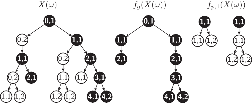
Remark 3.1. To understand why we include the third entry in the triple $(i_k,j_k,y_k)$ when we define the process on the Ulam–Harris space (see page 5), suppose we removed it; then, for $\omega$ illustrated in Figure 1, we have

\begin{equation*}f_g(\langle 0,1 \rangle ;\,1, \langle 0,2 \rangle ;\,1,\langle 1,1\rangle )=f_g(\langle 0,1 \rangle ;\,1,\langle 1,1\rangle )=(\langle 0,1 \rangle ;\,1, \langle 1,1 \rangle ),\end{equation*}

causing both individuals in generation one of $f_g(X(\omega))$ to have the same label. This makes the construction of the lineages in the next generation unclear.

We denote the probability-generating function of the offspring distribution of individuals in generation k of $\{ \textbf{\textit{Y}}_k \}$ by $\textbf{\textit{g}}_k(\textbf{\textit{s}}^{(d)})=(g_{k,i}(\textbf{\textit{s}}^{(d)}))_{1\leq i\leq d}$ , where $\textbf{\textit{s}}^{(d)} \in [0,1]^d$ . For $\ell\leq k$ we let $\textbf{\textit{g}}_{\ell\rightarrow k}(\textbf{\textit{s}}^{(d)})\,:\!= \textbf{\textit{g}}_\ell \circ \textbf{\textit{g}}_{\ell+1}\circ\cdots \circ\textbf{\textit{g}}_k(\textbf{\textit{s}}^{(d)})$ .

Lemma 3.1. For any $k\geq 0$ , $\textbf{\textit{g}}_k(\!\cdot\!)$ satisfies

(9) \begin{equation}{g}_{k,i}\big(\textbf{\textit{s}}^{(d)}\big)=G_{ \langle k,i \rangle}\big(\textbf{\textit{g}}_{0 \to k}\big(\textbf{\textit{s}}^{(d)}\big), \textbf{\textit{g}}_{1 \to k}\big(\textbf{\textit{s}}^{(d)}\big), \dots , \textbf{\textit{g}}_k\big(\textbf{\textit{s}}^{(d)}\big),\textbf{\textit{s}}^{(d)}, 1,1,\dots \big).\end{equation}

Proof. The proof follows the same conditioning argument as the proof of Lemma 3 in [Reference Braunsteins and Hautphenne7] but in the multitype setting.

We now show that the matrices $\{\mathcal{M}_k\}$ and $\{\mathcal{A}_k\}$ correspond to the first and second factorial moment progeny matrices in $\{\textbf{\textit{Y}}_k\}$ .

Lemma 3.2. If ${\tilde{\textbf{\textit{q}}}}=\textbf{1}$ , then, for any $k\geq 0$ ,

\begin{equation*}\mathcal{M}_k(i,j) = \left. \frac{\partial {g}_{k,i}(\textbf{\textit{s}}^{(d)})}{\partial s^{(d)}_{j}} \right|_{\textbf{\textit{s}}^{(d)}=\textbf{1}} \quad \mbox{ and } \quad \mathcal{A}_k(i;\,j,l) = \left. \frac{\partial^2 {g}_{k,i}(\textbf{\textit{s}}^{(d)})}{\partial s^{(d)}_{j} \partial s^{(d)}_{l}} \right|_{\textbf{\textit{s}}^{(d)}=\textbf{1}}.\end{equation*}

Proof. By (8) and the assumption ${\tilde{\textbf{\textit{q}}}}=\textbf{1}$ , we have $|\textbf{\textit{Y}}_k|<\infty$ almost surely (a.s.) for all k. Thus, $\textbf{\textit{g}}_{\ell\to k} (\textbf{1} )=\textbf{1}$ for all $\ell\leq k$ and $k\geq 0$ . The statement then follows by successive differentiations of (9).

Proof of Theorem 2.1. By Lemma 3.2, assertion (6) follows from (7) and [Reference Dolgopyat, Hebbar, Koralov and Perlman8, Proposition 2.1(e) and Theorem 2.1].

To obtain (5), we embed a second process in $\{ \textbf{\textit{Z}}_n \}$ , this time with the mean progeny matrix $M^{(k)}$ defined in (4). To do this we introduce a function $f_{p,k}(\!\cdot\!)\,:\, \mathcal{J} \to \mathcal{J}$ that takes a (possibly infinite) line of descent $(\varphi_0;\,i_1,j_1,{ y_1};\, i_2 , j_2, y_2,\dots)$ , and operates in two stages: first, it deletes the descendants of all triples $(i_\ell, j_{\ell}, y_\ell)$ whose level is strictly larger than k, to obtain the corresponding line of descent in $\big\{ {\tilde{\textbf{\textit{Z}}}}_n^{(T_{k})} \big\}$ ; and second, it deletes all remaining triples whose level differs from k to obtain the restriction (see [Reference Latouche and Ramaswami14, p. 118]) of $\big\{ {\tilde{\textbf{\textit{Z}}}}_n^{(T_{k})} \big\}$ to level k. When the function $f_{p,k}(\!\cdot\!)$ is applied to a random tree X, the result is a random tree which evolves as a d-type Galton–Watson process; see the right tree in Figure 1 as an example. In addition, if $\mathcal{M}_j<\infty$ for all $j=0,\dots, k-1$ , the mean progeny matrix of this embedded process is indeed given by $M^{(k)}$ . By irreducibility, with probability 1 this embedded process endures extinction if and only if $\big\{ \tilde{\textbf{\textit{Z}}}_n^{(T_{k})}\big\}$ does as well. Invoking the extinction criterion for finite-type processes (see, for instance, [Reference Harris10, Chapter II, Theorem 7.1]), $\tilde{\textbf{\textit{q}}}^{(T_{k})} =\textbf{1}$ if and only if ${\rm sp}(M^{(k)}) \leq 1$ . Thus, if ${\rm sp}(M^{(k)})<1$ for all $k\geq 0$ , then $\tilde{\textbf{\textit{q}}}^{(T_{k})} =\textbf{1}$ for all k, and according to [Reference Braunsteins and Hautphenne7, Theorem A.1] we then have ${\tilde{\textbf{\textit{q}}}}=\textbf{1}$ . Similarly, if there exists k such that ${\rm sp}(M^{(k)}) >1$ then $\tilde{\textbf{\textit{q}}}^{(T_{k})} <\textbf{1}$ and ${\tilde{\textbf{\textit{q}}}}\leq {\tilde{\textbf{\textit{q}}}}^{(T_{k})}<\textbf{1}$ . Finally, if there exists k such that ${\rm sp}(M^{(k)})=1$ , then by irreducibility there exists a path from level k to itself via a maximum level $\ell >k$ in the mean progeny representation graph of M, which again leads to ${\tilde{\textbf{\textit{q}}}}\leq {\tilde{\textbf{\textit{q}}}}^{(T_{\ell})}<\textbf{1}$ .

4. Extinction in sets of types

4.1. Extinction criteria

We now shift our attention to the more general extinction probability vectors $\textbf{\textit{q}}(A)$ ; in particular, we investigate how to determine when $\textbf{\textit{q}}(A)$ differs from $\textbf{\textit{q}}$ and ${\tilde{\textbf{\textit{q}}}}$ . We begin with a general result that allows us to use $q_{0,i}(A)$ , the probability that a type-i individual has no descendants in A, to compare extinction probability vectors.

Theorem 4.1. Let $A,B \subseteq \mathcal{X}_d$ . If $\sup_{i \in B} {q}_{0,i}(A)<1$ then $\textbf{\textit{q}}(A) \leq \textbf{\textit{q}}(B)$ .

Proof. Let $\mathcal{F}_n$ denote the history of the process up to generation n. By Lévy’s 0–1 law, for any fixed $\ell \geq 0$ ,

(10) \begin{equation}\mathbb{P}( \mathcal{E}_\ell(A) \mid \mathcal{F}_n ) \to { \mathrm{1}}(\mathcal{E}_\ell(A))\qquad \mbox{as $n \to \infty$}\end{equation}

on a subset $\Omega^*_{\ell}$ of the sample space that has probability 1. Let $\Omega^* = \bigcap_{\ell \geq 0} \Omega^*_{\ell}$ . For any outcome $\omega \in \bar{\mathcal{E}}(B) \cap \Omega^*$ (such that $\{ \textbf{\textit{Z}}_n(\omega) \}$ contains individuals with types in B for infinitely many n), we have $\mathbb{P}( \mathcal{E}_\ell(A) \mid \mathcal{F}_n)(\omega) < 1 - \varepsilon$ for infinitely many n, and for some $\varepsilon>0$ . Thus, by (10), $\mathrm{1}(\mathcal{E}_\ell(A))(\omega)<1-\varepsilon$ , that is, $\omega \in \bar{\mathcal{E}}_{\ell}(A)$ . Since this holds for all $\ell$ , $\omega \in \bigcup_{\ell \geq 0} \bar{\mathcal{E}}_\ell(A) = \bar{\mathcal{E}}(A)$ . Hence, $\mathcal{E}(A)\cap \bar{\mathcal{E}}(B) \subseteq \bar{\Omega}^*$ , leading to

\begin{equation*}\mathbb{P}_i(\mathcal{E}(A)) = \mathbb{P}_i\left(\mathcal{E}(A) \cap\mathcal{E}(B) \right) + \mathbb{P}_i\left(\mathcal{E}(A) \cap \bar{\mathcal{E}}(B)\right) \leq \mathbb{P}_i( \mathcal{E}(B))\end{equation*}

for any $i \in \mathcal{X}_d$ .

Corollary 4.1. Let $A \subseteq \mathcal{X}_d$ . If $\{\textbf{\textit{Z}}_n \}$ is irreducible then $ \textbf{\textit{q}}(A)\leq {\tilde{\textbf{\textit{q}}}}$ , and if in addition $|A| < \infty$ then $\textbf{\textit{q}}(A)= {\tilde{\textbf{\textit{q}}}}$ .

Proof. We first show that if $|A|<\infty$ , then $\textbf{\textit{q}}(A)= {\tilde{\textbf{\textit{q}}}}$ . By irreducibility, the condition of Theorem 4.1 is satisfied for any finite sets A and B. Thus, letting $B=T_k$ , we have $\textbf{\textit{q}}(A) = \textbf{\textit{q}}(T_k)$ for all $k \geq 0$ . Because $\mathcal{E}(T_{k+1}) \subseteq \mathcal{E}(T_{k})$ , by the monotone convergence theorem,

\begin{equation*} \textbf{\textit{q}}(A)=\lim_{k \to \infty} \textbf{\textit{q}}(T_k)=\mathbb{P}\left(\lim_{k \to \infty}\mathcal{E}(T_{k})\right)= \tilde{\textbf{\textit{q}}}.\end{equation*}

Now, for any $A \subseteq \mathcal{X}_d$ (not necessarily finite) and $i \in A$ we have $\textbf{\textit{q}}(A) \leq \textbf{\textit{q}}(\{ i \} ),$ and by what precedes, $\textbf{\textit{q}}(\{ i \} )= \tilde{\textbf{\textit{q}}}$ , therefore $ \textbf{\textit{q}}(A)\leq {\tilde{\textbf{\textit{q}}}}$ .

Given Corollary 4.1 we will focus on extinction in infinite sets A. In particular, we shall consider sets A belonging to the sigma algebra generated by the phase partition $\{ A_i \}$ , which we denote by $\sigma(A_1, \dots, A_d)$ . As we will see, even with just two phases ( $d=2$ ), it is possible for a process to survive in phase one, $A_1$ , while enduring extinction in phase two, $A_2$ , and vice versa. A concrete example is provided in Section 5. Nonetheless, the following result states that if the phases are sufficiently intertwined, then the probability of extinction in any set $A \in\sigma(A_1, \dots, A_d)$ coincides with the global extinction probability.

Corollary 4.2. If $\sup_{\ell \in A_i} {q}_{0,\ell}(A_j)< 1$ for all $i,j \in \{ 1, \dots, d \}$ then $\textbf{\textit{q}}(A)=\textbf{\textit{q}}$ for any $A \in \sigma(A_1, \dots, A_d)$ .

Proof. Since $d<\infty$ ,

\begin{equation*}\sup_{\ell \in A_i} {q}_{0,\ell}(A_j)< 1 \text{ for all } i,j \in \{ 1, \dots, d \} \Rightarrow \sup_{i \in \mathcal{X}_d} {q}_{0,i}(A) < 1 \text{ for any } A \in \sigma(A_1, \dots, A_d).\end{equation*}

The statement then follows from Theorem 4.1.

Corollaries 4.1 and 4.2 indicate that, under quite general conditions, $\textbf{\textit{q}}(A)={\tilde{\textbf{\textit{q}}}}$ if $|A|<\infty$ and $\textbf{\textit{q}}(A)=\textbf{\textit{q}}$ if $|A|=\infty$ , the same as in the single-phase LHBP analysed in [Reference Braunsteins and Hautphenne7]. So, when do we have $\textbf{\textit{q}} < \textbf{\textit{q}}(A)< \tilde{\textbf{\textit{q}}}$ ? We begin with a necessary condition, which follows from Theorem 2.1.

Corollary 4.3. If $\textbf{\textit{q}} < \textbf{\textit{q}}(A)$ then

(11) \begin{equation}{\tilde{\textbf{\textit{q}}}}^{( \bar{A})} <\textbf{1}.\end{equation}

Corollary 4.3 states that to have $\textbf{\textit{q}} < \textbf{\textit{q}}(A)$ , it must be possible for $\{ \textbf{\textit{Z}}_n \}$ to survive in the types $\bar A$ without any outside assistance from the types in A. To verify (11), we observe that when $A \in \sigma(A_1, \dots,A_d)$ , $\tilde M^{(\bar A)}$ is block lower Hessenberg; we can then compute the sequence $\{ \tilde{\mathcal{M}}_k ^{( \bar A)} \}_{ k \geq 0} $ using (3) with $\tilde{M}^{(\bar A)}$ substituted for M, and apply Theorem 2.1. The matrices $\{ \tilde{\mathcal{M}}_k^{(\bar A)} \}$ are also a fundamental ingredient in Theorem 4.2. In preparation for this theorem, for each level $k\geq 0$ we let $\bar{A}(k)=\bar A \cap L_k$ , and we define

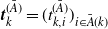
1. • the column vector $\textbf{\textit{t}}_k^{({\bar{A}})}=(t_{k,i}^{(\bar{A})})_{i\in \bar{A}(k)}$ , where

   \begin{equation*}t_{k,i}^{(\bar{A})} \,:\!= \sum_{ j \in A} M({ i} , j)\end{equation*}
   is the expected total number of direct descendants in A from a parent of type $\langle k,i \rangle \in \bar{A}$ , and

2. • the matrix $\tilde F_k^{(\bar{A})}=(\tilde F_k^{(\bar{A})}(i,j))_{i, j \in \bar{A}(k)}$ , where $\tilde F_k^{(\bar{A})}(i,i)\,:\!=1, $ and where, for $i\neq j$ ,

   \begin{equation*}\tilde F_k^{(\bar{A})}(i,j) \,:\!= M^{(\bar{A})}(i , j)+\displaystyle{\sum_{\substack{k\geq 1\\ i_1,i_2, \dots, i_{k} \neq j}}}\tilde M^{(\bar{A})}(i , i_1)\tilde M^{(\bar{A})}(i_1,i_2) \cdots \tilde M^{(\bar{A})}(i_k,j)\end{equation*}
   is the weighted sum of first passage paths from i to j in level k in the mean progeny representation graph of $\tilde M^{(A)}$ .

We also let $\tilde{\mathcal{M}}^{(\bar{A})}_{0\rightarrow k-1}\,:\!=\mathcal{M}_0^{(\bar A)}\mathcal{M}_1^{(\bar A)} \cdots \mathcal{M}_{k-1}^{(\bar A)}$ , and v be the number of phases in $\bar A$ so that $v = |\bar A(k)|$ for all k.

Theorem 4.2. Let $A \in \sigma(A_1, \dots, A_d)$ , and assume ${\tilde{\textbf{\textit{q}}}}^{(\bar{A})}<\textbf{1}$ and $\nu(\tilde{M}^{(\bar{A})}) <1$ . If, in addition,

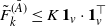
1. (A) $\sum^{\infty}_{k=0} \big(\textbf{1}_v^\top \textbf{\textit{t}}_k^{(\bar A)}\big) \,\tilde{ \mathcal{M}}^{(\bar{A})}_{0\rightarrow k-1} \textbf{1}_v < \infty, $ and

2. (B) there exists $K<\infty$ such that $\tilde F_k^{(\bar A)} \leq K\, \textbf{1}_v\cdot\textbf{1}_v^\top$ for all $k \geq 0$ ,

then $\textbf{\textit{q}} < \textbf{\textit{q}}(A)$ and $\textbf{\textit{q}}(\bar A) <\tilde{\textbf{\textit{q}}}$ .

Proof. We first demonstrate that, under the conditions of the theorem, the expected number of sterile individuals produced over the lifetime of $\Big\{ {\tilde{\textbf{\textit{Z}}}}_n^{(\bar{A})} \Big\}$ (those with type in A) is finite. Without loss of generality we assume that the process starts with an individual of type $i\in \bar A(0)$ . Let $\tilde M^{(\bar{A},n)}( i ,j)$ denote the (i, j)th entry of the nth power of $\tilde M^{(\bar{A})}$ . The expected number of sterile types produced throughout the lifetime of $\{ {\tilde{\textbf{\textit{Z}}}}_n^{(\bar{A})} \}$ is then given by

(12) \begin{align}\mathbb{E}_{i} \left( \sum_{n=0}^\infty \sum_{l \in A} \tilde{Z}_{n,l}^{({ \bar{A}})} \right) & = \sum_{k=0}^\infty \sum_{j\in \bar{A}(k)} \sum_{n=0}^\infty \tilde M^{(\bar{A},n)}( i ,j) \,t_{k,j}^{(\bar{A})}.\end{align}

Observe that for any $k \geq 0$ , $ i \in\bar{A}(0)$ , and $j\in \bar{A}(k)$ , we have

(13) \begin{align}\sum^\infty_{n =0} \tilde M^{(\bar{A},n)}( i ,j) &=\sum_{l \in \bar{A}(k)} \tilde{\mathcal{M}}^{(\bar{A})}_{0\rightarrow k-1} (i,l)\, F_k^{(\bar{A})}(l,j)\,\sum^\infty_{n =0} \tilde M^{(\bar{A},n)}( j ,j) \nonumber\\[5pt] &\leq\left( \frac{1}{1-\nu(\tilde{M}^{(\bar{A})}) }\right) \left[\tilde{\mathcal{M}}^{(\bar{A})}_{0\rightarrow k-1}\, F_k^{(\bar{A})}\right](i,j),\end{align}

where (13) follows from [Reference Seneta17, Theorem A4]. By (12), (13), and the assumptions of the theorem, we then have, in matrix form,

\begin{align*}\mathbb{E}_{\bar{A}(0)} \left( \sum_{n=0}^\infty \sum_{l \in A} \tilde{Z}_{n,l}^{({ \bar{A}})}\right) &\leq \left( \frac{1}{1-\nu(\tilde{M}^{(\bar{A})}) }\right) \sum_{k=0}^\infty \tilde{\mathcal{M}}^{(\bar{A})}_{0\rightarrow k-1}\, \tilde F_k^{(\bar A)} \textbf{\textit{t}}_k^{(\bar A)} \\[3pt] &\leq \left( \frac{K}{1-\nu(\tilde{M}^{(\bar{A})}) }\right) \sum_{k=0}^\infty ( \textbf{1}_v^\top \textbf{\textit{t}}_k^{(\bar A)} )\,\tilde{\mathcal{M}}^{(\bar{A})}_{0\rightarrow k-1} \textbf{1}_v \\[3pt] &<\infty.\end{align*}

Because this expectation is finite, with probability 1 there exists a generation n after which a sterile type in A never appears in the population. Thus, under the assumption ${\tilde{\textbf{\textit{q}}}}^{(\bar{A})}<\textbf{1}$ , there exists a type $i \in \bar A$ such that starting from i there is a positive chance of global survival without entering the set A. By Theorem 1.1 we then have $\textbf{\textit{q}} < \textbf{\textit{q}}(A)$ . In addition, by the assumption $\nu\big(\tilde{M}^{(\bar{A})}\big) <1$ , if $\{ \textbf{\textit{Z}}_n \}$ survives in $\bar A$ but not in A, then it becomes partially extinct with probability 1, leading to $\textbf{\textit{q}}(\bar A) <\tilde{\textbf{\textit{q}}}$ .

If for some set $B \in \sigma(A_1, \dots , A_d)$ the conditions of Theorem 4.2 hold with both $A=B$ and $A=\bar B$ , then $\textbf{\textit{q}}< \textbf{\textit{q}}(B) < \tilde{\textbf{\textit{q}}}$ and $\textbf{\textit{q}}< \textbf{\textit{q}}(\bar B) < \tilde{\textbf{\textit{q}}}$ . Condition (A) of Theorem 4.2 can be verified easily if there are only finitely many edges between A and $\bar{A}$ in the mean progeny representation graph of M, because in that case there are only finitely many values of k such that $\textbf{\textit{t}}_k^{(\bar A)}$ is nonzero. Condition (B) of Theorem 4.2 is of a more technical nature. It holds, for example, if $\bar A$ contains a single phase, or if the phases in $\bar A$ are sufficiently intertwined, or if there is some symmetry between the phases. The next lemma formalises this.

Lemma 4.1. If $\nu(\tilde M^{(\bar A)})<1$ then each of the following conditions is sufficient for Condition (B):

1. (B1) $\bar A=A_i$ for some $i\in\{1,\ldots,d\}$ .

2. (B2) There exists $\varepsilon >0$ such that $\tilde F_k^{(\bar A)}( i,j) > \varepsilon$ for all $i,j \in \bar A(k)$ and $k \geq 0$ .

3. (B3) For any $k,\ell \geq 0$ , $i\in \bar A(k)$ , and $j\in \bar A(\ell)$ , we have $\tilde M^{(\bar A)}( i,j ) = \tilde M^{(\bar A)}( j,i )$ .

Proof. The sufficiency of (B1) is trivial since then $\tilde F^{(\bar A)}=1$ . The sufficiency of (B2) and (B3) follows from the fact that when $\nu(\tilde M^{(\bar A)}) < 1$ , for any $k\geq 0$ and $i,j\in\bar A(k)$ , $\tilde F^{(\bar A)}(i,j)\tilde F^{(\bar A)}(j,i)$ is bounded above by the weighted sum of first return paths from i to i in the mean progeny representation graph of M, which is strictly less than 1.

In the specific case where $\{ \textbf{\textit{Z}}_n \}$ is singular, that is, each individual produces exactly one offspring with probability 1, the process survives with probability 1 ( $\textbf{\textit{q}}=\textbf{0}$ ), and the process $\{Z_n\}_{n\geq 0}$ , where ${Z}_n\,:\!=i\Leftrightarrow {Z}_{n,i}>0$ , corresponds to an irreducible Markov chain on the state space $\mathcal{X}_d$ . The arguments in the proof of Theorem 4.2 then lead to the following corollary, which can be viewed as the algorithmic complement to the more theoretical result of [Reference van Doorn19, Corollary 8].

Corollary 4.4. If $| \textbf{\textit{Z}}_n| = 1$ a.s. for all $n \geq 0$ , then

(14) \begin{equation}\textbf{\textit{q}}(A)>\textbf{0} \quad \Leftrightarrow \quad \lim_{k \to \infty} \textbf{1}_v^\top \left( \prod_{j=k}^\infty \tilde{\mathcal{M}}_j^{(\bar{A})}\right)\textbf{1}_v >0.\end{equation}

In addition, if $\sum_{x\in\bar A(k+1)} \tilde M^{(\bar A)}( \langle k,i \rangle, x) > 0$ for all $\langle k , i \rangle \in \bar A$ , then the right-hand side of (14) may be replaced by 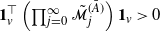$\textbf{1}_v^\top \left( \prod_{j=0}^\infty \tilde{\mathcal{M}}_j^{(\bar{A})}\right)\textbf{1}_v>0$ .

Proof. By Theorem 1.1, $\textbf{\textit{q}}(A)>\textbf{0} $ if and only if there exists $i\in\bar{A}$ such that the probability that the chain $\{Z_n\}$ never visits A starting from i is strictly positive, which is equivalent to the right-hand side of (14). The additional condition $\sum_{x\in\bar A(k+1)} \tilde M^{(\bar A)}( \langle k,i \rangle, x) > 0$ for all $\langle k , i \rangle \in \bar A$ ensures that there is no null factor in the product $\prod_{j=0}^\infty \tilde{\mathcal{M}}_j^{(\bar{A})}$ .

4.2. Computational methods

Given the existence of extinction probability vectors $\textbf{\textit{q}}(A)$ different from $\textbf{\textit{q}}$ and ${\tilde{\textbf{\textit{q}}}}$ , we now develop a method of computing them.

For any $k, \ell\geq -1$ , define the finite-type branching process $\{ \textbf{\textit{Z}}^{(k,\ell)}_n(A)\}$ on the same probability space as $\{ \textbf{\textit{Z}}_n \}$ , in which individuals give birth according to the probability-generating function ${\textbf{\textit{G}}}^{(k,\ell)}(A)(\textbf{\textit{s}})$ such that

\begin{equation*}{G}_i^{(k,\ell)}(A)(\textbf{\textit{s}})= \begin{cases}0, \quad & \text{if } i \in A \cap \bar T_k , \\[3pt] 1, \quad & \text{if } i \in \bar A \cap \bar T_{\ell} , \\[3pt] G_i( \textbf{\textit{s}}) \quad & \text{otherwise},\end{cases}\end{equation*}

and denote by $\textbf{\textit{q}}^{(k,\ell)}(A)$ its extinction probability vector. In other words, $\textbf{\textit{q}}^{(k,\ell)}(A)$ is the probability that the branching process $\{ {\tilde{\textbf{\textit{Z}}}}_n^{(A \cup T_\ell)} \}$ becomes extinct before producing a type in $A \cap \bar T_k$ (with $T_{-1}=\varnothing$ and $\bar T_{-1}=\mathcal{X}_d$ ). For any k and $\ell$ , the vector $\textbf{\textit{q}}^{(k,\ell)}(A)$ can then be computed using established techniques for finite-type branching processes.

Theorem 4.3. If $\{ \textbf{\textit{Z}}_n \}$ is irreducible then

\begin{equation*}\lim_{k \to \infty} \lim_{\ell \to \infty} \textbf{\textit{q}}^{(k,\ell)}(A)= \textbf{\textit{q}}(A).\end{equation*}

Proof. By Theorem A.1 of [Reference Braunsteins and Hautphenne7], for any fixed value of k, $\lim_{\ell \to \infty} \textbf{\textit{q}}^{(k,\ell)}(A)$ is the partial extinction probability of the original process modified so that types in $A \cap \bar T_k$ are immortal. Let

\begin{equation*} N(A)\,:\!= \inf \left\{ N\geq 0 \,:\, \sum_{n=N}^\infty \sum_{i \in A} Z_{n,i}> 0 \right\} \end{equation*}

be the last generation at which a type in A appears in the population, and

(15) \begin{equation}\tau_k(A)\,:\!= \inf \left\{k\geq 0\,:\, \sum_{n=0}^k \sum_{i \in A \bigcap \bar T_k} Z_{n,i}> 0 \right\}\end{equation}

be the first generation at which a type in $A \cap \bar T_k$ appears in the population. By Corollary 4.1 and the fact that $|A \cap T_k |< \infty$ for all k, we have, for all $i\in\mathcal{X}_d$ ,

\begin{align*} \lim_{\ell \to \infty} {q}_i^{(k,\ell)}(A)&=\mathbb{P}_i \left({ \{ N(A) < \tau_k(A) \} \bigcap \left\{ \bigcap_{u=1}^\infty \mathcal{E}\left(\bar A \cap T_u\right)\right\}}\right) \\ &=\mathbb{P}_i \left( \{ N(A) < \tau_k(A) \} \right). \end{align*}

By the monotone convergence theorem we then have

\begin{align*}\lim_{k \to \infty} \mathbb{P}_i ( \{ N(A) < \tau_k(A) \}) & = \mathbb{P}_i ( \{ N(A) < \lim_{k \to \infty} \tau_k(A) \}) \\ & = \mathbb{P}_i (N(A) < \infty ) \\ & = \mathbb{P}_i (\mathcal{E}(A)),\end{align*}

which concludes the proof.

Following the arguments in the proof of Theorem 4.3, we obtain a method to compute the probability $\textbf{\textit{q}}_0(A)$ that no individuals with type in A will ever be produced:

Corollary 4.5. If $\{ \textbf{\textit{Z}}_n \}$ is irreducible then

\begin{equation*} \lim_{\ell \to \infty} \textbf{\textit{q}}^{({-}1,\ell)}(A)= \textbf{\textit{q}}_0(A).\end{equation*}

While Theorem 4.3 may be applied in a general setting, it requires both k and $\ell$ to be increased to infinity separately. From a computational perspective it would be more efficient to set $\ell = k$ and let them both increase to infinity together. We now derive a sufficient condition ensuring convergence of the resulting sequence.

Theorem 4.4. If $\sup_{i \in A } \tilde{q}_i^{(A)}<1$ then

\begin{equation*} \lim_{k \to \infty} \textbf{\textit{q}}^{(k,k)}(A) = \textbf{\textit{q}}(A). \end{equation*}

Proof. First, suppose that $\{ \textbf{\textit{Z}}_n \}$ becomes extinct in the set A. In this case, there exists K such that $\tau_k(A)=\infty$ for all $k >K$ , where $\tau_k(A)$ is defined in (15). In addition, by Theorem 4.1 there is almost sure partial extinction. This implies that for $k>K$ there is almost sure global extinction in $\{ \textbf{\textit{Z}}_n^{(k,k)}(A) \}$ , leading to $\textbf{\textit{q}}(A) \leq \liminf_k \textbf{\textit{q}}^{(k,k)}(A)$ .

Now suppose that $\{ \textbf{\textit{Z}}_n \}$ survives in the set A. At any generation n, consider the daughter processes of each individual in $( Z_{n,i})_{i \in A}$ truncated so that all types in $\bar A$ have no offspring. Note that if one of these truncated daughter processes survives globally, then there exists K such that $Z^{(k,k)}(A)$ survives globally for all $k>K$ . This is because for these values of k an immortal type $A \cap \bar T_k$ must eventually be born into the population. Let D be the event that, throughout the life of $\{ \textbf{\textit{Z}}_n \}$ , there exists an individual that has a truncated daughter process which survives globally. By assumption, there exists $\varepsilon >0$ such that, whenever $( Z_{n,i})_{i \in A}$ is nonempty, we have $\mathbb{P} (D \mid \mathcal{F}_n ) > \varepsilon$ . Because $\{ \textbf{\textit{Z}}_n \}$ survives in the set A, $( Z_{n,i})_{i \in A}$ is nonempty for infinitely many values of n. Therefore, following the same arguments as in the proof of Theorem 4.1, the event D occurs with probability 1. This then implies $\textbf{\textit{q}}(A) \geq \limsup_k \textbf{\textit{q}}^{(k,k)}(A)$ .

To understand why we impose the sufficient condition $\sup_{i \in A } \tilde{q}^{(A)}_i<1$ in Theorem 4.4, consider an example with two phases where this condition is not satisfied. Assume ${\textbf{\textit{G}}}( \textbf{\textit{s}})$ contains entries

\begin{equation*}G_{\langle k, i \rangle}( \textbf{\textit{s}} ) = \begin{cases}s_{\langle k+1, 1 \rangle} s_{\langle 0, 2 \rangle}, \quad & \langle k, i \rangle \in A_1 , \\[5pt] \frac{ k+1}{ k+2}s_{\langle k+1,2 \rangle} + \frac{1}{ k+2}, \quad & \langle k, i \rangle \in A_2.\end{cases}\end{equation*}

In this case, $q_{\langle 0 ,1\rangle}(A_2)= 0$ but $q^{(k,k)}_{\langle 0 ,1 \rangle}(A_2) = \big(1- \frac{1}{k+2}\big)^{k+1} \to {\rm e}^{-1}$ . While this is a reducible example, it highlights a pathology that can also occur in the irreducible setting.

4.3. Fixed points

We now briefly turn our attention to the set S, which contains the extinction probability vectors $\textbf{\textit{q}}(A)$ . To allow the results on (single-phase) LHBPs provided in [Reference Braunsteins and Hautphenne7, Section 4] to be applied directly, we introduce the concept of a block LHBP that is locally isomorphic to a (single-phase) LHBP. Roughly speaking, this is a block LHBP which takes the distribution of an LHBP when we sum the number of individuals in each level (i.e. $ \big(\sum_{j \in L_k} Z_{n,j}\big)_{k \geq 0}\stackrel{{\rm d}}{=} {\hat{\textbf{\textit{Z}}}}_n,$ where $\{ {\hat{\textbf{\textit{Z}}}}_n \}$ is an LHBP). More specifically, $\{\textbf{\textit{Z}}_n \}$ is locally isomorphic to an LHBP $\{ {\hat{\textbf{\textit{Z}}}}_n \}$ if, for each level $k \geq 0$ , there exists a probability distribution $\hat p_k(\!\cdot\!) \,:\, R_{k,1} \to [0,1]$ such that, for any $\textbf{\textit{u}} \in R_{k,1}$ and $j \in L_k$ ,

\begin{equation*} \hat p_k(\textbf{\textit{u}}) = \sum_{ \substack{ \textbf{\textit{r}}\in R_{k,d} \,s.t.\\ \sum_{x \in L_i} r_x=u_i \, \forall i}} p_j( \textbf{\textit{r}}).\end{equation*}

We define the projection of S onto the kth level:

\begin{equation*}S_{k} \,:\!= \{ \textbf{\textit{u}} \in [0,1]^{d} \,:\, \text{there exists } \textbf{\textit{s}} \in S \text{ with } (s_j)_{j\in L_k} = \textbf{\textit{u}} \}.\end{equation*}

The next proposition is the irreducible block analogue of [Reference Braunsteins and Hautphenne7, Theorem 4.1].

Proposition 4.1. Suppose $\{ \textbf{\textit{Z}}_n \}$ is locally isomorphic to an LHBP that satisfies the conditions of [Reference Braunsteins and Hautphenne7, Theorem 4.1]. Then

\begin{equation*}\textbf{\textit{q}}=\min S,\qquad{\tilde{\textbf{\textit{q}}}} = \sup S \backslash \{ \textbf{1} \},\end{equation*}

and

\begin{equation*} (x q_{\langle k,1\rangle} + (1 - x) \tilde{q}_{\langle k, 1 \rangle }) \textbf{1}_{d} \in S_{k} \qquad \mbox{ for all } x \in [0,1],\end{equation*}

where $q_{\langle k,1\rangle}=\cdots=q_{\langle k,d\rangle}$ , and $\tilde{q}_{\langle k, 1 \rangle }=\cdots=\tilde{q}_{\langle k, d \rangle }.$

Proof. Let $\textbf{\textit{s}}= [0,1]^{\mathcal{X}_1}$ and suppose $\textbf{\textit{s}} = \hat{\textbf{\textit{G}}}( \textbf{\textit{s}} )$ . Then, for any $k \geq 0$ and any $j \in L_k$ ,

\begin{align*}{G}_j(s_0 \textbf{1}_{d}, s_1 \textbf{1}_{d}, \dots) &= \sum_{\textbf{\textit{u}} \in R_{k,d}} (s_0 \textbf{1}_{d}, s_1 \textbf{1}_{d}, \dots)^{\textbf{\textit{u}}} p_j(\textbf{\textit{u}}) \\&= \sum_{\textbf{\textit{u}} \in R_{k,1}} \textbf{\textit{s}}^{\textbf{\textit{u}}} \left( \sum_{\textbf{\textit{v}} \,:\, u_i = \sum_{x \in L_i} v_x, \, \forall i} p_j( \textbf{\textit{v}}) \right) \\&= \sum_{\textbf{\textit{u}} \in R_{k,1}} \textbf{\textit{s}}^{\textbf{\textit{u}}} \hat p_k( \textbf{\textit{u}} ) =s_k.\end{align*}

Therefore,

\begin{equation*}(s_0 \textbf{1}_{d}, s_1 \textbf{1}_{d}, \dots) = {\textbf{\textit{G}}}(s_0 \textbf{1}_{d}, s_1 \textbf{1}_{d}, \dots),\end{equation*}

and the result follows as a direct consequence of [Reference Braunsteins and Hautphenne7, Theorem 4.1].

Remark 4.1. Blackwell [Reference Blackwell4] demonstrated that, if $\{\textbf{\textit{Z}}_n \}$ is singular (so $\textbf{\textit{q}}=\textbf{0}$ ) and $\tilde{\textbf{\textit{q}}}=\textbf{1}$ , then there are two distinct extinction probability vectors if and only if every bounded solution to $\textbf{\textit{s}}={\textbf{\textit{G}}}(\textbf{\textit{s}})$ is of the form $\textbf{\textit{s}} =c\textbf{1}$ for $c \geq 0$ . In the context of this section, this means that if $\{\textbf{\textit{Z}}_n \}$ is singular then $\textbf{\textit{q}}(A) \in \{ \textbf{\textit{q}}, \tilde{\textbf{\textit{q}}} \}$ for all $A \subseteq \mathcal{X}$ if and only if $S_k$ is entirely made up of the linear segment identified in Proposition 4.1. The next example suggests that this criterion does not generalise to nonsingular branching processes.

5. Illustrations

We now illustrate our main theorems through two examples, and motivate some open questions.

Example 5.1. We consider a two-phase ( $d=2$ ) block LHBP with ${\textbf{\textit{G}}}( \textbf{\textit{s}} )$ given by

\begin{equation*}G_{\langle k,i \rangle}(\textbf{\textit{s}})= \begin{cases}\frac{b}{u}s_{\langle 0,i \rangle}^u+\frac{c}{u}s_{\langle 1,i \rangle}^u +\frac{y}{u}s_{\langle 0, 3-i \rangle}^u +1-\frac{b+c+y}{u}, \quad & k=0,\\[5pt] \frac{a}{u}s_{\langle k-1,i \rangle}^u+\frac{b}{u}s_{\langle k,i \rangle}^u+\frac{c}{u}s_{\langle k+1,i \rangle}^u & \\[5pt] \qquad\;\;\;\;\;\;\,\,\,+\frac{y}{u x^k}s_{\langle k, 3-i \rangle}^u +1-\frac{a+b+c+y x^{-k}}{u}, \, \, & k \geq 1 ,\end{cases}\end{equation*}

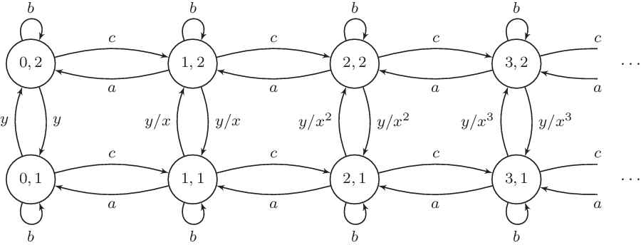
for $i=1,2$ , where $a,b,c,y>0$ , $x\geq 1$ , and $u=\lceil a+b+c+y +1 \rceil$ . Observe that, in this example, individuals produce either u offspring or no offspring. The corresponding mean progeny representation graph is illustrated in Figure 2.

Figure 2:

The mean progeny representation graph corresponding to Example 5.1.

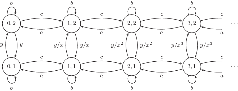
In this example, the processes $\big\{ \tilde{\textbf{\textit{Z}}}_n^{(A_1)} \big\}$ and $\big\{ \tilde{\textbf{\textit{Z}}}_n^{(A_2)} \big\}$ restricted to each phase form stochastically identical nearest-neighbour branching random walks with an absorbing barrier [Reference Biggins, Lubachevsky, Shwartz and Weiss3]. Individuals within the same level give birth to each other with a probability that decays geometrically at rate x with the individual’s level. We can also verify that the process is locally isomorphic to an LHBP $\{ \hat{\textbf{\textit{Z}}}_n \}$ . The next proposition highlights the contrasting asymptotic behaviours of the branching process as a function of the decay rate x.

Proposition 5.1. Suppose $b+2\sqrt{ac}<1$ and

\begin{equation*} \mu\,:\!= \left(1-b - \sqrt{(1-b)^2-4ac} \right)/2a >1. \end{equation*}

We have:

1. (i) If $x=1$ and $b+y+2\sqrt{ac} \leq 1$ , then $\textbf{\textit{q}}=\textbf{\textit{q}}(A_1)=\textbf{\textit{q}}(A_2)<{\tilde{\textbf{\textit{q}}}}=\textbf{1}$ .

2. (ii) If $x=1$ and $b+y+2\sqrt{ac} > 1$ , then $\textbf{\textit{q}}=\textbf{\textit{q}}(A_1)=\textbf{\textit{q}}(A_2)={\tilde{\textbf{\textit{q}}}}<\textbf{1}$ .

3. (iii) If $x>1$ , then $\textbf{\textit{q}}<{\tilde{\textbf{\textit{q}}}}$ .

4. (iv) If $x>\mu$ , then $\textbf{\textit{q}}< \textbf{\textit{q}}(A_1)<{\tilde{\textbf{\textit{q}}}}$ and $\textbf{\textit{q}}< \textbf{\textit{q}}(A_2)<{\tilde{\textbf{\textit{q}}}}$ .

Proof. (i) and (ii). Suppose $x=1$ . By Corollary 4.2, $\textbf{\textit{q}}=\textbf{\textit{q}}(A_1)=\textbf{\textit{q}}(A_2)$ , and by [Reference Braunsteins and Hautphenne7, Corollary 3], $\textbf{\textit{q}}<\textbf{1}$ . Note that there is partial (global) extinction in $\{ \textbf{\textit{Z}}_n \}$ if any only if there is partial (global) extinction in its local isomorphism $\{ \hat{\textbf{\textit{Z}}}_n \}$ . Denote the mean progeny matrix of $\{ \hat{\textbf{\textit{Z}}}_n \}$ by $\hat M$ . This is a tridiagonal matrix with entries $\hat M(i,i-1) =a \textbf{1}\{ i \geq 1\}$ , $\hat M(i,i)=b+y$ , $\hat M(i,i+1)=c$ for $i \geq 0$ , and 0 otherwise. By [Reference Hautphenne, Latouche and Nguyen11, Proposition 5.1], $\nu(\hat M)=b+y+2\sqrt{ac}$ , which means

\begin{equation*}{\tilde{\textbf{\textit{q}}}} = \textbf{1} \quad \Leftrightarrow \quad b+y+2\sqrt{ac} \leq 1 ,\end{equation*}

yielding (i). Observe that when $x=1$ , $\{ \hat{\textbf{\textit{Z}}}_n \}$ is a branching random walk with an absorbing barrier, which implies that $\tilde q_{\langle k , i \rangle }$ is decreasing in k. Consequently, when $b+ y + 2\sqrt{ac} >1$ the entries of ${\tilde{\textbf{\textit{q}}}}$ are uniformly bounded away from 1. By [Reference Moyal15, Lemma 3.3], S contains only one such element, which, when combined with the fact that $\textbf{\textit{q}}\leq \tilde{\textbf{\textit{q}}}$ , yields (ii).

(iii). Suppose $x>1$ . Let $\wideparen M^{(\bar T_k)} = (\wideparen M^{(\bar T_k)}(i,j) )_{i,j \geq 1}$ , where $\wideparen M^{(\bar T_k)}(i,j) \,:\!= \hat M (\langle i + k,1 \rangle, \langle j+k,1 \rangle)$ , is the mean progeny matrix of the process $\{ \hat{\textbf{\textit{Z}}}_n \}$ taboo on $T_k$ (which we denote by $\big\{ \wideparen{\textbf{\textit{Z}}}^{(\bar T_k)}_n \big\}$ ), with entries relabelled for convenience. It is such that $\wideparen M^{(T_k)}(i,i)=b+y/x^{k+i}$ , $\wideparen M^{(T_k)}(i,i+1)=c$ for $i\geq 1$ , and $\wideparen M^{(T_k)}(i,i-1)=a$ for $i\geq 2$ . We have $b\leq b+y/x^{k+i}\leq b+y/x^{k+1}$ for all k, i; therefore, by the definition of the convergence norm, and by [Reference Hautphenne, Latouche and Nguyen11, Proposition 5.1], $b + 2\sqrt{ac}\leq \nu\big( \wideparen M^{(\bar T_k)} \big)\leq b+y/x^{k+1} + 2\sqrt{ac}$ for all k, leading to

\begin{equation*}\lim_{k \to \infty} \nu\big( \wideparen M^{(\bar T_k)} \big) = b + 2\sqrt{ac}<1.\end{equation*}

In addition, by [Reference Braunsteins and Hautphenne7, Corollary 3], for any $k \geq 0$ and initial type $i \in \bar T_k$ , $\Big\{ \wideparen{\textbf{\textit{Z}}}^{(\bar T_k)}_n \Big\}$ has a positive chance of global survival. The assertion then follows through direct application of [Reference Braunsteins and Hautphenne7, Theorem 7.1].

(iv). Suppose $x>\mu$ . We have $t_k^{(A_1)}=y/x^k$ and, by [Reference Braunsteins and Hautphenne7, Lemma 9], $\tilde{\mathcal{M}}_k^{(A_1)} \to \mu$ . Thus,

\begin{equation*}\lim_{k \to \infty} \left(\tilde{\mathcal{M}}^{(A_1)}_{0\rightarrow k-1}\,t_k^{(A_1)}\,\right)^{1/k} =\mu/x<1.\end{equation*}

The root test for convergence then gives $ \sum_{k=0}^\infty \tilde{\mathcal{M}}^{(A_1)}_{0\rightarrow k-1}\,t_k^{(A_1)}<\infty$ . By [Reference Braunsteins and Hautphenne7, Corollary 3] and [Reference Hautphenne, Latouche and Nguyen11, Proposition 5.1] we have ${\tilde{\textbf{\textit{q}}}}^{(A_1)}< \textbf{1}$ and $\nu\big( \tilde{M}^{(A_1)}\big)=b + 2\sqrt{ac}<1$ . By Theorem 4.2 we have $\textbf{\textit{q}}<\textbf{\textit{q}}(A_2)$ and $\textbf{\textit{q}}(A_1)<\tilde{\textbf{\textit{q}}}$ . The result then follows by repeating the same arguments with $A_2$ in place of $A_1$ .

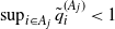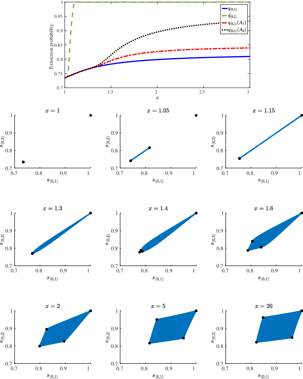
We let $a=1/5$ , $b=0$ , $c=1$ , and $y=1/5$ , and we study the extinction probabilities for different values of the parameter x. In this case, $b+y+2\sqrt{ac}\approx 1.09$ and $\mu \approx 1.38$ . Here, $\sup_{i \in A_j } \tilde{q}^{(A_j)}_i<1$ for $j=1,2$ , therefore we can use Theorem 4.4 to compute $\textbf{\textit{q}}(A_1)$ and $\textbf{\textit{q}}(A_2)$ . The top graph in Figure 3 depicts the extinction probabilities $q_{\langle 0,1 \rangle}$ , $q_{\langle 0,1 \rangle}(A_1)$ , $q_{\langle 0,1 \rangle}(A_2)$ , and $\tilde q_{\langle 0,1 \rangle}$ for $1\leq x\leq 3$ . As Proposition 5.1 suggests, we observe two phase transition points, the first at $x=1$ , where the number of distinct extinction probability vectors increases from one to two (even if it only becomes clear slightly after $x=1$ ), and the second at $x=\mu$ , where the number of distinct extinction probability vectors increases from two to four. By visual inspection, there exists an infimum value of x for which ${\tilde{\textbf{\textit{q}}}} =\textbf{1}$ . Using Theorem 2.1. we numerically estimate this value to be approximately $1.09$ .

Figure 3:

Example 5.1. Top: The extinction probabilities $q_{\langle 0,1 \rangle}$ , $q_{\langle 0,1 \rangle}(A_1)$ , $q_{\langle 0,1 \rangle}(A_2)$ , and $\tilde q_{\langle 0,1 \rangle}$ for $1\leq x\leq 3$ . Bottom: The projection set $S_{0}$ for nine values of x.

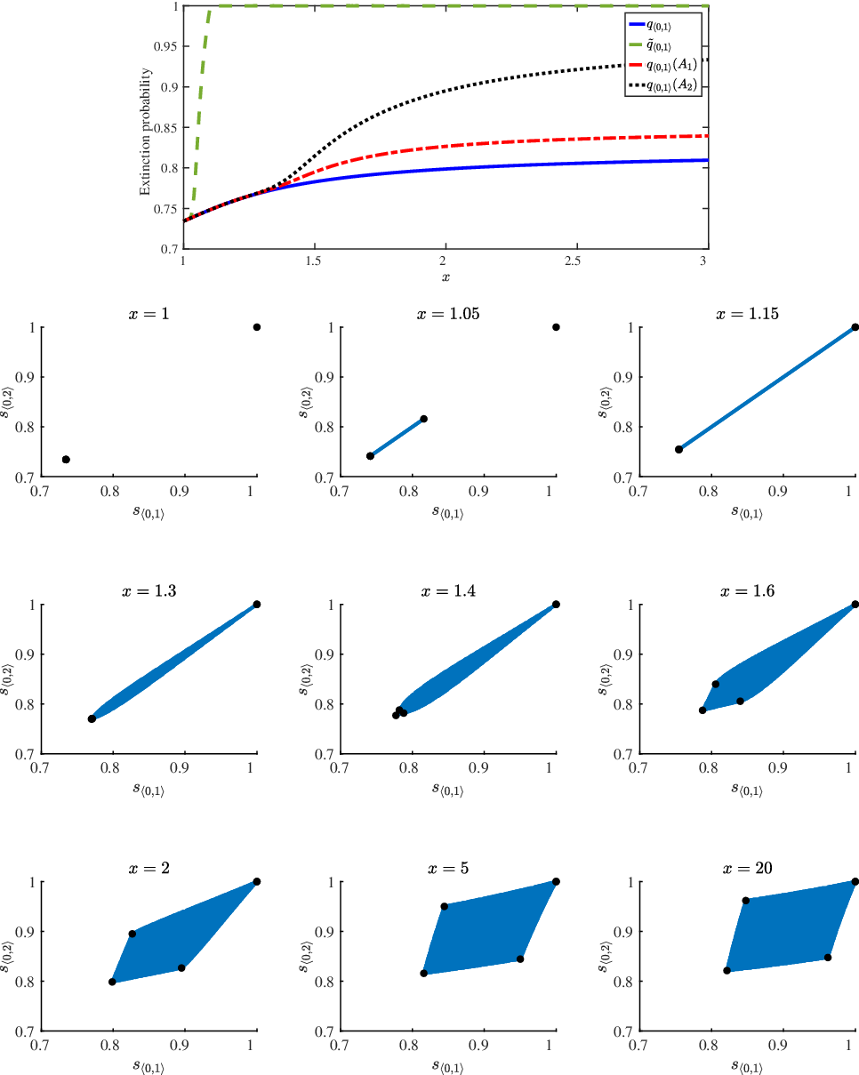
The bottom nine graphs in Figure 3 illustrate the set $S_{0}$ (S projected onto level 0) for nine values of x ranging from $x=1$ to $x=20$ . The projected extinction probabilities $(q_{\langle 0,1 \rangle}, q_{\langle 0,2 \rangle })$ , $(q_{\langle 0,1 \rangle}(A_1), q_{\langle 0,2 \rangle}(A_1))$ , $(q_{\langle 0,1 \rangle}(A_2),$ $q_{\langle 0,2 \rangle}(A_2))$ , and $(\tilde q_{\langle 0,1 \rangle}, \tilde q_{\langle 0,2 \rangle})$ are marked by bold discs. We observe that for small values of x (i.e. $x=1,1.05,1.1$ ) the elements in $S_0$ cling tightly to the straight line of fixed points connecting $\textbf{\textit{q}}$ and $\tilde{\textbf{\textit{q}}}$ that we identified in Proposition 4.1. As x increases, the set $S_{0}$ inflates until it visibly contains area. Noticeably, this occurs when $x\leq \mu$ (i.e. $x=1.2$ ; see Remark 4.1) as well as when $x>\mu$ . For large values of x (i.e. $x=5,20$ ), the extinction probabilities $(q_{\langle 0,1 \rangle}(A_1), q_{\langle 0,2 \rangle}(A_1))$ and $(q_{\langle 0,1 \rangle}(A_2), q_{\langle 0,2 \rangle}(A_2))$ appear to correspond to vertices in $S_{0}$ , while this is less clear for smaller values of $x>\mu$ (i.e. $x=1.4,1.6$ ).

Due to the symmetry of the progeny distributions between phases 1 and 2, the level projection sets $S_k$ are symmetric with respect to the diagonal. The next example considers an asymmetric modification of Example 5.1.

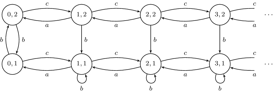
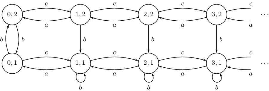
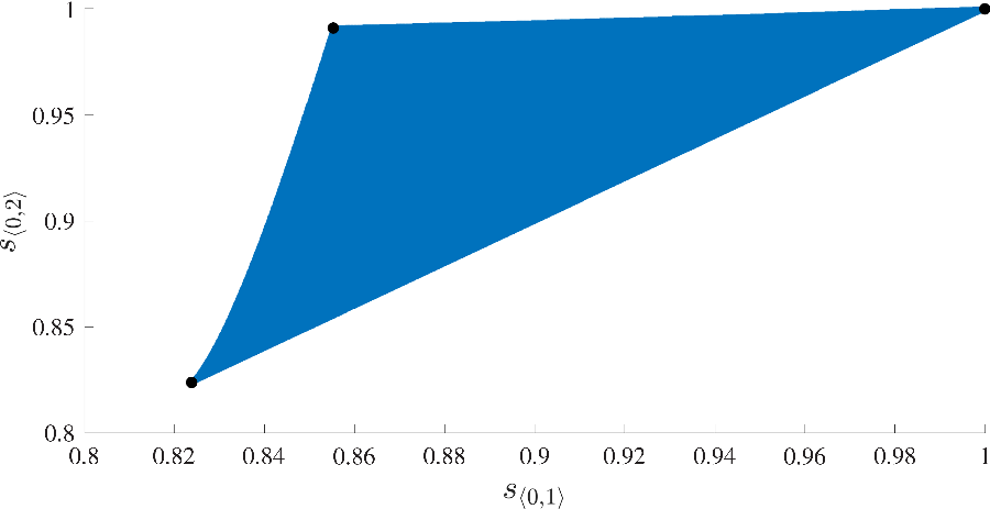
Example 5.2. We modify Example 5.1 such that the mean progeny representation graph becomes as shown in Figure 4. In Figure 5 we plot the set $S_0$ for $a=1/5$ , $b=1/20$ , and $c=1$ , and observe that there are only three distinct extinction probability vectors, $\textbf{\textit{q}}$ , $\textbf{\textit{q}}(A_2)$ , and ${\tilde{\textbf{\textit{q}}}}$ . Indeed, by Corollary 4.2, $\textbf{\textit{q}}(A_1) = \textbf{\textit{q}}$ . Despite the lack of symmetry, this branching process is still locally isomorphic to a single-phase LHBP. 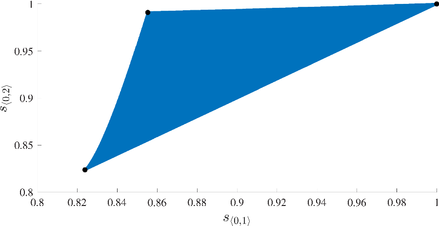Thus, by Proposition 4.1, the set $S_0$ still contains the linear segment that connects the global and partial extinction probabilities, $(q_{\langle 0,1 \rangle} , q_{\langle 0 ,2 \rangle})$ and $(\tilde q_{\langle 0,1 \rangle} , \tilde q_{\langle 0 ,2 \rangle})$ . On inspection of Figure 5 we see that this linear segment now sits on the boundary of $S_0$ .

Figure 4:

Mean progeny representation graph corresponding to Example 5.2.

Figure 5:

The projection set $S_{0}$ corresponding to Example 5.2.

Examples 5.1 and 5.2 motivate several questions, which to our knowledge remain open. In particular:

1. (i) We have only focused on sets $A \in \sigma(A_1, \dots, A_d)$ , leading to a maximum of $2^d-1$ potentially distinct extinction probability vectors ${\textbf{\textit{q}}(A)}$ (if we exclude $\textbf{\textit{q}}(\emptyset)=\textbf{1}$ ). We may then ask if more than $2^d$ (including ${\tilde{\textbf{\textit{q}}}}$ ) distinct extinction probability vectors can exist in an irreducible block LHBP when we consider any $A \subseteq \mathcal{X}_d$ .

2. (ii) Given the set S, we may question whether it is possible to identify which elements correspond to extinction probability vectors.

We now propose an answer to (ii), which we suggest applies to any irreducible multitype Galton–Watson branching process with countably many types: