1 Introduction
1.1 Brief overview
This paper is concerned with properties of the velocity gradient tensor (VGT) for incompressible, homogeneous, isotropic turbulence (HIT). This is a classical topic in turbulence fluid mechanics as HIT is the testing ground for a great deal of turbulence theory as the equations for the evolution for the VGT are derived by taking the spatial gradient of the Navier–Stokes equations. Hence, as studies of the VGT refine knowledge of flow structure topologies, distortion and their interaction with dissipation (Tsinober, Shtilman & Vaisburd Reference Tsinober, Shtilman and Vaisburd1997), the physical understanding of the cascades of energy and enstrophy are enhanced, leading to new conceptual models (Lundgren Reference Lundgren1982; Goto Reference Goto2008) and better prospects for practical modelling of turbulent flows. A recent review paper by Meneveau (Reference Meneveau2011) provides a great deal of information on the properties of the VGT and serves as both a basis and a point of departure for this study. The key difference concerns the form of decomposition of the tensor. Conventional studies employ the clearly physically interpretable Hermitian/skew-Hermitian decomposition into strain,
 $\unicode[STIX]{x1D64E}$
, and rotation,
 $\unicode[STIX]{x1D734}$
, components, with the latter often then expressed as a vorticity vector. However, the eigenvalues of the VGT are also important for delimiting different topological states of the tensor, and therefore there is some history to studying the invariants of the characteristic equation for the VGT (Kerr Reference Kerr1985; Ashurst et al.
Reference Ashurst, Kerstein, Kerr and Gibson1987; Cantwell Reference Cantwell1993; Jeong & Girimaji Reference Jeong and Girimaji2003; Elsinga & Marusic Reference Elsinga and Marusic2010; Paul, Papadakis & Vassilicos Reference Paul, Papadakis and Vassilicos2017), as well as modelling their evolution (Girimaji & Pope Reference Girimaji and Pope1990; Cantwell Reference Cantwell1992; Martin, Dopazo & Valiño Reference Martin, Dopazo and Valiño1998; Nomura & Post Reference Nomura and Post1998; Biferale et al.
Reference Biferale, Chevillard, Meneveau and Toschi2007; Li & Meneveau Reference Li and Meneveau2007). The approach proposed here attempts to unify both eigenvalue and strain/rotation frameworks and, as a consequence, helps elucidate important aspects of the flow physics.
The first thing noted is that just examining the eigenvalues is insufficient for developing an alternative decomposition of the VGT. While the Hermitian/skew-Hermitian decomposition gives an additive decomposition of the velocity gradient tensor,
 $\unicode[STIX]{x1D63C}$
:
 $$\begin{eqnarray}\unicode[STIX]{x1D63C}=\unicode[STIX]{x1D64E}+\unicode[STIX]{x1D734},\end{eqnarray}$$
to form the equivalent with an eigenvalue-based approach, a decomposition of the tensor into a normal tensor,
 $\unicode[STIX]{x1D63D}$
, (characterized by the eigenvalues) and a non-normal part,
 $\unicode[STIX]{x1D63E}$
, (characterizing the tensor asymmetries) is needed. Hence, an alternative to (1.1) may be written as
 $$\begin{eqnarray}\unicode[STIX]{x1D63C}=\unicode[STIX]{x1D63D}+\unicode[STIX]{x1D63E}.\end{eqnarray}$$
The tool from matrix algebra used to accomplish this is the Schur transform (Schur Reference Schur1909). Having commenced the analysis of
 $\unicode[STIX]{x1D63C}$
from this starting point, the Hermitian/skew-Hermitian decompositions of
 $\unicode[STIX]{x1D63D}$
and
 $\unicode[STIX]{x1D63E}$
can be used to elucidate the relative importance of strain and rotation for both the normal and non-normal parts of the tensor. This framework may then be employed to re-interrogate and shed further light on a number of properties of the VGT.
The plan of this manuscript is to review key mathematical and physical aspects of the velocity gradient tensor in the remainder of the introduction, establishing concepts to be used as the basis or point of departure for the Schur approach. In § 2 we then introduce the Schur decomposition and use it to derive the decomposition in (1.2). Taking the strain and rotation components of these tensors permits the core concepts from the introduction to be stated in a new way (§§ 2.2 and 2.3), and allows derivation of the evolution equations for strain and rotation in this framework (§ 2.4). The final two parts of § 2 use the derived terms to formulate metrics to characterize the physical aspects of the tensor that are employed in the results sections. The first results, in § 4, concern the importance of non-normality for the tensor in terms of norms, enstrophy, strain and the respective production terms. Section 5 then examines the strain rate tensor to show how turbulence forms disc-like structures. Finally, § 6 re-interrogates vorticity vector and strain eigenvector alignments to explain the preferential alignment between the vorticity vector and the eigenvector for the intermediate strain eigenvalue.
1.2 The velocity gradient tensor and the invariants of its characteristic equation
The velocity gradient tensor,
 $\unicode[STIX]{x1D63C}\in \text{Re}^{3\times 3}$
, is given by
 $\unicode[STIX]{x1D608}_{ij}=\unicode[STIX]{x2202}u_{i}/\unicode[STIX]{x2202}x_{j}$
, where
 $u$
is a velocity component and
 $x$
is a spatial direction. It is directly related to the Navier–Stokes equations,
 $$\begin{eqnarray}\frac{\unicode[STIX]{x2202}}{\unicode[STIX]{x2202}t}\boldsymbol{u}+\boldsymbol{u}\boldsymbol{\cdot }\unicode[STIX]{x1D735}\boldsymbol{u}=-\frac{1}{\unicode[STIX]{x1D70C}}\unicode[STIX]{x1D735}p+\unicode[STIX]{x1D708}\unicode[STIX]{x0394}\boldsymbol{u},\end{eqnarray}$$
where
 $t$
is time,
 $p$
is the pressure,
 $\unicode[STIX]{x1D70C}$
is the density and
 $\unicode[STIX]{x1D708}$
is the kinematic viscosity. This may be made explicit by taking the spatial gradient of the Navier–Stokes equations:
 $$\begin{eqnarray}\frac{\unicode[STIX]{x2202}}{\unicode[STIX]{x2202}t}\unicode[STIX]{x1D63C}+\boldsymbol{u}\boldsymbol{\cdot }\unicode[STIX]{x1D735}\unicode[STIX]{x1D63C}=-\unicode[STIX]{x1D63C}^{2}-\unicode[STIX]{x1D643}+\unicode[STIX]{x1D708}\unicode[STIX]{x0394}\unicode[STIX]{x1D63C},\end{eqnarray}$$
where
 $\unicode[STIX]{x1D643}$
is the Hessian of the kinematic pressure field, i.e.
 $\unicode[STIX]{x1D60F}_{ij}=\unicode[STIX]{x2202}^{2}p/\unicode[STIX]{x2202}x_{i}\unicode[STIX]{x2202}x_{j}$
. The characteristic equation for
 $\unicode[STIX]{x1D63C}$
is
 $$\begin{eqnarray}\unicode[STIX]{x1D706}_{i}^{3}+\unicode[STIX]{x1D64B}_{A}\unicode[STIX]{x1D706}_{i}^{2}+\unicode[STIX]{x1D64C}_{A}\unicode[STIX]{x1D706}_{i}+\unicode[STIX]{x1D64D}_{A}=0,\end{eqnarray}$$
where the
 $\unicode[STIX]{x1D706}_{i}$
are the eigenvalues of the tensor. Clearly, the three invariants of this equation may be expressed in terms of the eigenvalues and for an incompressible flow, because there is zero trace,
 $\text{tr}(\unicode[STIX]{x1D63C})=0$
, and
 $\unicode[STIX]{x1D64B}_{A}=\sum \unicode[STIX]{x1D706}_{i}$
, it follows that
 $\unicode[STIX]{x1D64B}_{A}=0$
. The second and third invariants,
 $\unicode[STIX]{x1D64C}_{A}$
and
 $\unicode[STIX]{x1D64D}_{A}$
are given by:
 $$\begin{eqnarray}\displaystyle & \displaystyle \unicode[STIX]{x1D64C}_{A}=-\frac{1}{2}\text{tr}(\unicode[STIX]{x1D63C}^{2})\equiv (1-\unicode[STIX]{x1D6FF}_{ij})\sum \unicode[STIX]{x1D706}_{i}\unicode[STIX]{x1D706}_{j} & \displaystyle\end{eqnarray}$$
 $$\begin{eqnarray}\displaystyle & \displaystyle \unicode[STIX]{x1D64D}_{A}=-\text{det}(\unicode[STIX]{x1D63C})\equiv \prod \unicode[STIX]{x1D706}_{i}, & \displaystyle\end{eqnarray}$$
where
 $\unicode[STIX]{x1D6FF}_{ij}$
is the Kronecker delta. These expressions for
 $\unicode[STIX]{x1D64C}_{A}$
and
 $\unicode[STIX]{x1D64D}_{A}$
are of significance topologically, because the sign of the discriminant function for incompressible flow
 $$\begin{eqnarray}\unicode[STIX]{x1D6E5}_{L}=\unicode[STIX]{x1D64C}_{A}^{3}+{\textstyle \frac{27}{4}}\unicode[STIX]{x1D64D}_{A}^{2},\end{eqnarray}$$
separates regions where the eigenvalues form a conjugate pair (
 $\unicode[STIX]{x1D6E5}_{L}>0$
) and where they are all real (
 $\unicode[STIX]{x1D6E5}_{L}<0$
). In the Lagrangian frame of a moving fluid element, the former results in closed streamlines, explaining the use of
 $\unicode[STIX]{x1D6E5}_{L}>0$
as a local, practical tool for coherent structure identification (Chong, Perry & Cantwell Reference Chong, Perry and Cantwell1990), although because
 $\unicode[STIX]{x1D64C}_{A}$
is raised to an odd power in (1.8), it follows that
 $\unicode[STIX]{x1D64C}_{A}>0$
is a more restrictive definition (Hunt, Wray & Moin Reference Hunt, Wray and Moin1988; Dubief & Delcayre Reference Dubief and Delcayre2000). Because of this physical meaning to the change in eigenvalue behaviour, it follows that particular regions of joint
 $\unicode[STIX]{x1D64C}_{A}{-}\unicode[STIX]{x1D64D}_{A}$
space have topological interpretation (Perry & Chong Reference Perry and Chong1987):
(i)
 $\unicode[STIX]{x1D6E5}_{L}>0,\unicode[STIX]{x1D64D}_{A}>0$
– compressing of the flow towards an unstable focus region;
(ii)
$\unicode[STIX]{x1D6E5}_{L}>0,\unicode[STIX]{x1D64D}_{A}<0$
– stretching of the flow away from a stable focus region;(iii)
$\unicode[STIX]{x1D6E5}_{L}<0,\unicode[STIX]{x1D64D}_{A}>0$
– two saddles with an unstable node;(iv)
$\unicode[STIX]{x1D6E5}_{L}<0,\unicode[STIX]{x1D64D}_{A}<0$
– two saddles with a stable node.


Alternatively,
 $\unicode[STIX]{x1D64C}_{A}$
and
 $\unicode[STIX]{x1D64D}_{A}$
can be defined in terms of strain and rotation tensors. A Hermitian/skew-Hermitian decomposition into strain and rotation is given by
 $$\begin{eqnarray}\displaystyle & \displaystyle \unicode[STIX]{x1D64E}_{A}={\textstyle \frac{1}{2}}(\unicode[STIX]{x1D63C}+\unicode[STIX]{x1D63C}^{\ast }) & \displaystyle\end{eqnarray}$$
 $$\begin{eqnarray}\displaystyle & \displaystyle \unicode[STIX]{x1D734}_{A}={\textstyle \frac{1}{2}}(\unicode[STIX]{x1D63C}-\unicode[STIX]{x1D63C}^{\ast }) & \displaystyle\end{eqnarray}$$
where the
 $\ast$
superscript is the conjugate transpose. This leads to
 $$\begin{eqnarray}\displaystyle \unicode[STIX]{x1D64C}_{A} & = & \displaystyle {\textstyle \frac{1}{2}}(\Vert \unicode[STIX]{x1D734}_{A}\Vert ^{2}-\Vert \unicode[STIX]{x1D64E}_{A}\Vert ^{2})\nonumber\\ \displaystyle & & \displaystyle \equiv \unicode[STIX]{x1D64C}_{A}^{(\unicode[STIX]{x1D6FA})}-\unicode[STIX]{x1D64C}_{A}^{(S)}\end{eqnarray}$$
 $$\begin{eqnarray}\displaystyle \unicode[STIX]{x1D64D}_{A} & = & \displaystyle -\text{det}(\unicode[STIX]{x1D64E}_{A})-\text{tr}(\unicode[STIX]{x1D734}_{A}^{2}\unicode[STIX]{x1D64E}_{A})\nonumber\\ \displaystyle & & \displaystyle \equiv \unicode[STIX]{x1D64D}_{A}^{(S)}-\text{tr}(\unicode[STIX]{x1D734}_{A}^{2}\unicode[STIX]{x1D64E}_{A}),\end{eqnarray}$$
where, e.g.
 $\Vert \unicode[STIX]{x1D64E}_{A}\Vert =\sqrt{\text{tr}(\unicode[STIX]{x1D64E}_{A}\unicode[STIX]{x1D64E}_{A}^{\ast })}$
is the Frobenius norm and one may also choose to work with the vorticity vector,
 $\unicode[STIX]{x1D74E}$
, where each element is
 $$\begin{eqnarray}\unicode[STIX]{x1D714}_{i}=-\unicode[STIX]{x1D716}_{ijk}\unicode[STIX]{x1D6FA}_{jk},\end{eqnarray}$$
and
 $\unicode[STIX]{x1D716}_{ijk}$
is the Levi-Cevita symbol. Equations (1.11) and (1.12) give physical interpretations of the invariants as the excess of enstrophy with respect to total strain and the excess of strain production with respect to enstrophy production, respectively. It should be noted that while
 $\unicode[STIX]{x1D64C}_{A}$
is therefore the difference between two positive quantities,
 $\unicode[STIX]{x1D64D}_{A}$
reflects a balance between two terms, for which both mean values are positive (Taylor Reference Taylor1938; Betchov Reference Betchov1956), but the instantaneous values may take either sign. This provided the motivation for Lüthi and co-workers to examine the velocity gradient tensor from the perspective of a
 $\unicode[STIX]{x1D64C}_{A};-\text{det}(\unicode[STIX]{x1D64E}_{A});\text{tr}(\unicode[STIX]{x1D734}_{A}^{2}\unicode[STIX]{x1D64E}_{A})$
decomposition (Lüthi, Holzner & Tsinober Reference Lüthi, Holzner and Tsinober2009).
The well-known
 $\unicode[STIX]{x1D64C}{-}\unicode[STIX]{x1D64D}$
diagram (
 $\unicode[STIX]{x1D64C}_{A}{-}\unicode[STIX]{x1D64D}_{A}$
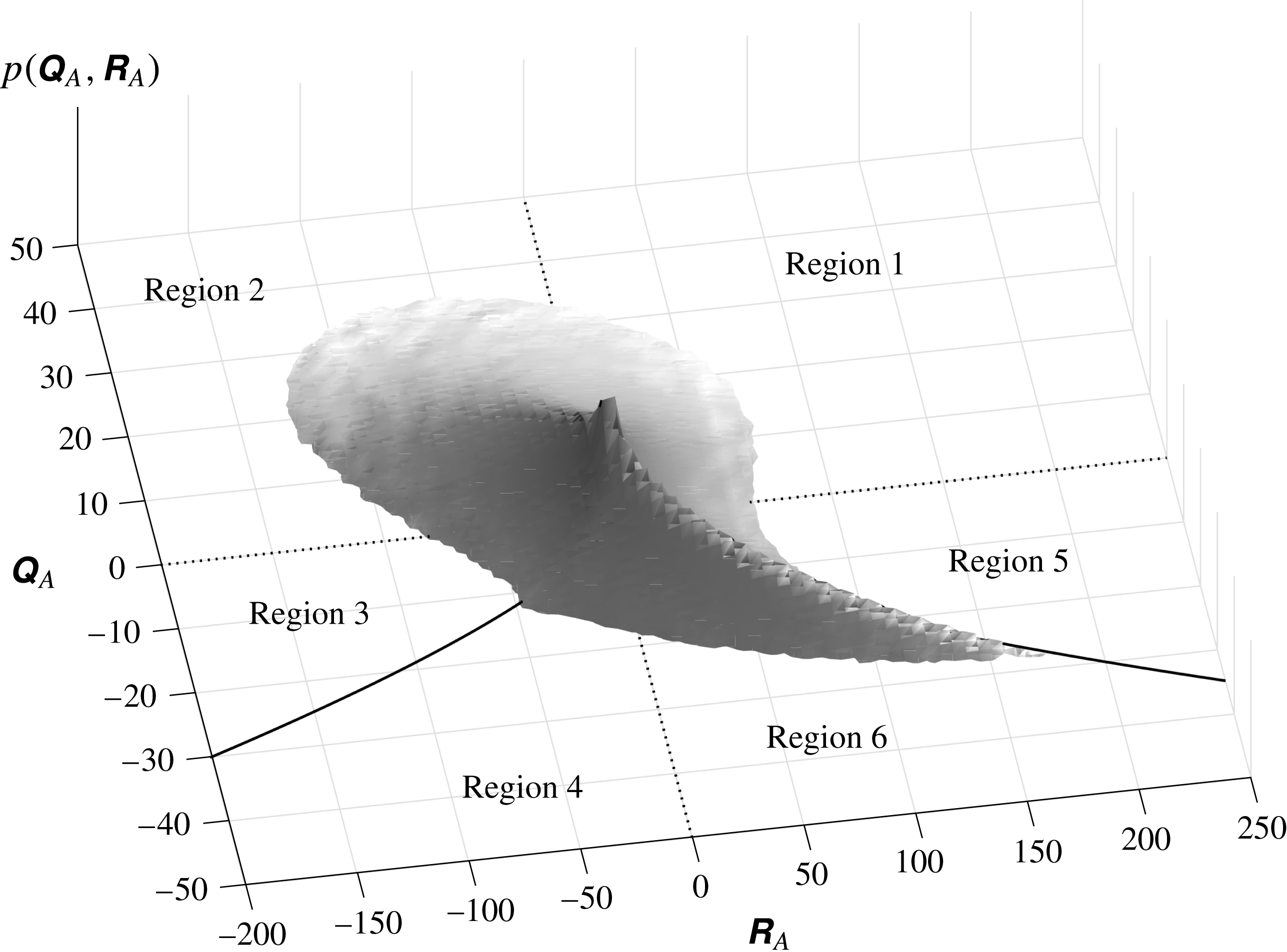
in this paper’s notation) is shown for homogeneous, isotropic turbulence (HIT) at a Taylor Reynolds number of 433 in figure 1, with the discriminant function,
 $\unicode[STIX]{x1D6E5}_{L}$
as a solid line and the six regions that are delimited throughout this study are also labelled. The features of this diagram are well known and of particular prominence is the Vieillefosse tail (Vieillefosse Reference Vieillefosse1984) that forms a ‘ridge’ to the joint distribution function on the positive
 $\unicode[STIX]{x1D64D}_{A}$
side. The degree of mass along the tail, close to the origin and in the opposite (
 $\unicode[STIX]{x1D64C}>0,\unicode[STIX]{x1D64D}<0$
) quadrant can be shown to be statistically significant features of HIT both with respect to Gaussian, random tensors (Tsinober Reference Tsinober, Hunt and Vassilicos2001) and random tensors constrained to local properties (Keylock Reference Keylock2017).
A schematic of the joint distribution function that forms the
 $\unicode[STIX]{x1D64C}_{A}{-}\unicode[STIX]{x1D64D}_{A}$
diagram, plotted as a surface, with the discriminant function,
 $\unicode[STIX]{x1D6E5}_{L}=0$
, shown as a solid line and the six regions used throughout this study highlighted. The Vieillefosse tail is the elongated feature between regions 5 and 6 close to where
 $\unicode[STIX]{x1D6E5}_{L}=0$
(Vieillefosse Reference Vieillefosse1984). This figure was constructed using the results stored in the Johns Hopkins database (Li et al.
Reference Li, Perlman, Wan, Yang, Burns, Meneveau, Chen, Szalay and Eyink2008).

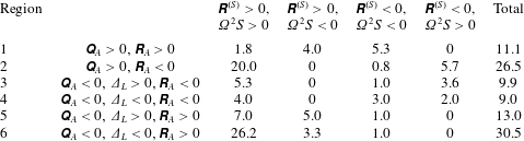
Occupancy (expressed as a percentage of realizations) of different states for HIT for the velocity gradient tensor,
 $\unicode[STIX]{x1D63C}$
. For compactness, the
 $A$
subscript is not used in the table headings. Hence,
 $\unicode[STIX]{x1D64D}^{(S)}\equiv -\text{det}(\unicode[STIX]{x1D64E}_{A})$
and
 $\unicode[STIX]{x1D6FA}^{2}S\equiv \text{tr}(\unicode[STIX]{x1D734}_{A}^{2}\unicode[STIX]{x1D64E}_{A})$
.

Table 1 summarizes how the velocity gradient tensors for HIT extracted from the Johns Hopkins database used to populate figure 1 are distributed over the six regions of the
 $\unicode[STIX]{x1D64C}_{A}{-}\unicode[STIX]{x1D64D}_{A}$
diagram and the four feasible states for enstrophy production and strain production. What is very clear is that the two most frequently occupied regions (regions 2 and 6), with opposite signs for
 $\unicode[STIX]{x1D64C}_{A}$
and
 $\unicode[STIX]{x1D64D}_{A}$
, are both dominated by positive strain production and enstrophy production. However, the relative magnitudes of these terms differ significantly in these two cases to establish the change in sign for
 $\unicode[STIX]{x1D64D}_{A}$
. The only region where tensors with negative values for both enstrophy production and strain production are more likely than tensors with both terms positive is region 1. The opposite region to this (region 4) has a nearly equal probability of the two strain/enstrophy production states, while in the regions adjacent to, but above, the discriminant function (regions 3 and 5) it is seen that the physically feasible combination with different signs for the two production terms is nearly as likely as the case where both are positive. Hence, these latter two regions exhibit intermediate characteristics compared to regions 2 and 4, and 1 and 6, respectively. These properties of the VGT are summarized here because much subsequent analysis highlights that the normal and non-normal properties of the tensor vary greatly between these regions.
An important study with regards to modelling the dynamics of the VGT is due to Cantwell (Reference Cantwell1992), who derived the restricted Euler equations assuming that viscosity could be ignored and that the pressure Hessian acted in an isotropic fashion:
 $$\begin{eqnarray}\displaystyle & \displaystyle \frac{\text{d}\unicode[STIX]{x1D64C}_{A}}{\text{d}t}=-3\unicode[STIX]{x1D64D}_{A} & \displaystyle\end{eqnarray}$$
 $$\begin{eqnarray}\displaystyle & \displaystyle \frac{\text{d}\unicode[STIX]{x1D64D}_{A}}{\text{d}t}=\frac{2}{3}\unicode[STIX]{x1D64C}_{A}^{2}. & \displaystyle\end{eqnarray}$$
There are two possible solutions. Given the time scale,
 $t_{0}=1/\sqrt{|\unicode[STIX]{x1D64C}_{A}^{0}|}$
, for
 $\unicode[STIX]{x1D64C}_{A}^{0}=0,\unicode[STIX]{x1D64D}_{A}<0$
the solutions evolve to the fixed point,
 $\unicode[STIX]{x1D64C}_{A}=\unicode[STIX]{x1D64D}_{A}=0$
. For any other initial conditions the solution evolves towards the Vieillefosse tail, defined as the bottom right quadrant of figure 1 along the line
 $\unicode[STIX]{x1D6E5}_{L}=0$
. That the majority of points lie close to the origin, or along the Vieillefosse tail in figure 1 highlights the relevance of the restricted Euler approximation to the Navier–Stokes problem. However, it is clearly necessary to go beyond this approach to derive a workable model for the velocity gradient tensor dynamics that includes terms that prevent the mass of the distribution function over-accumulating at the extreme of the Vieillefosse tail (Wilczek & Meneveau Reference Wilczek and Meneveau2014; Johnson & Meneveau Reference Johnson and Meneveau2016). This implies that, in addition to
 $\unicode[STIX]{x1D64C}_{A}$
and
 $\unicode[STIX]{x1D64D}_{A}$
, i.e. normal terms defined in terms of the eigenvalues, it is important to study how non-normality contributes to this dynamics, which is the emphasis of this paper. Thus, we define non-normality and develop our decomposition in the next section.
2 An additive decomposition of the velocity gradient tensor resolving normal and non-normal effects explicitly
2.1 Tensor non-normality and the Schur transform
This study proposes an additive decomposition of the velocity gradient tensor,
 $\unicode[STIX]{x1D63C}$
, into normal,
 $\unicode[STIX]{x1D63D}$
, and non-normal,
 $\unicode[STIX]{x1D63E}$
, components before any subsequent decomposition into rotation or strain tensors. This permits the unpacking of a number of phenomena commonly lumped together, clarifying the behaviour of the tensor.
If
 $\unicode[STIX]{x1D63C}$
is normal, then
 $$\begin{eqnarray}\unicode[STIX]{x1D63C}\unicode[STIX]{x1D63C}^{\ast }=\unicode[STIX]{x1D63C}^{\ast }\unicode[STIX]{x1D63C}.\end{eqnarray}$$
An eigenvalue decomposition is given by
 $$\begin{eqnarray}\unicode[STIX]{x1D647}\unicode[STIX]{x1D726}\unicode[STIX]{x1D647}^{-1}=\unicode[STIX]{x1D63C},\end{eqnarray}$$
where
 $\unicode[STIX]{x1D647}$
contains the eigenvectors and
 $\unicode[STIX]{x1D726}$
is a diagonal matrix of eigenvalues (
 $\unicode[STIX]{x1D6EC}_{1,1}=\unicode[STIX]{x1D706}_{1}$
). The Schur transform (Schur Reference Schur1909) is given by:
 $$\begin{eqnarray}\unicode[STIX]{x1D650}\unicode[STIX]{x1D64F}\unicode[STIX]{x1D650}^{\ast }=\unicode[STIX]{x1D63C},\end{eqnarray}$$
where
 $\unicode[STIX]{x1D650}$
is unitary and
 $\unicode[STIX]{x1D64F}=\unicode[STIX]{x1D726}+\unicode[STIX]{x1D649}$
, with
 $\unicode[STIX]{x1D649}$
a strictly upper triangular tensor for the complex Schur transform. That is, because the
 $\unicode[STIX]{x1D706}_{i}$
may contain a conjugate pair (where
 $\unicode[STIX]{x1D6E5}_{L}>0$
), to ensure
 $\unicode[STIX]{x1D649}$
is upper triangular rather than quasi-upper triangular, a complex Schur decomposition is used throughout this study (Golub & van Loan Reference Golub and van Loan2013). For a brief overview of formal properties of the Schur decomposition, see appendix A.
Clearly, because
 $\unicode[STIX]{x1D650}$
is unitary,
 $\unicode[STIX]{x1D650}\unicode[STIX]{x1D650}^{\ast }=\unicode[STIX]{x1D644}$
, where
 $\unicode[STIX]{x1D644}$
is the identity matrix, and this also implies
 $\unicode[STIX]{x1D650}\unicode[STIX]{x1D650}^{-1}=\unicode[STIX]{x1D644}$
. The eigenvalue decomposition sacrifices this unitarity of basis for diagonality of
 $\unicode[STIX]{x1D726}$
. Hence, informally, deviations of
 $\unicode[STIX]{x1D647}$
from a unitary form in an eigenvalue decomposition are reflected in
 $\unicode[STIX]{x1D649}$
in the Schur decomposition. Therefore, the advantage of the Schur decomposition is that it moves non-normal effects out of the eigenvectors (orientations) and into a tensor
 $\unicode[STIX]{x1D649}$
that may be additively coupled to the eigenvalues. From (2.1) and this discussion it follows that
 $\Vert \unicode[STIX]{x1D63C}\unicode[STIX]{x1D63C}^{\ast }-\unicode[STIX]{x1D63C}^{\ast }\unicode[STIX]{x1D63C}\Vert$
and
 $\Vert \unicode[STIX]{x1D649}\Vert$
are both measures of non-normality (Henrici Reference Henrici1962; Eberlein Reference Eberlein1965; Lee Reference Lee1995).
2.2 Normal and non-normal velocity gradient tensors and the invariants of the velocity gradient tensor
The normal and non-normal tensors may now be stated:
 $$\begin{eqnarray}\displaystyle & \displaystyle \unicode[STIX]{x1D63D}=\unicode[STIX]{x1D650}\unicode[STIX]{x1D726}\unicode[STIX]{x1D650}^{\ast } & \displaystyle\end{eqnarray}$$
 $$\begin{eqnarray}\displaystyle & \displaystyle \unicode[STIX]{x1D63E}=\unicode[STIX]{x1D650}\unicode[STIX]{x1D649}\unicode[STIX]{x1D650}^{\ast }, & \displaystyle\end{eqnarray}$$
and this is the key conceptual innovation in this paper. Thus, there is an additive decomposition,
 $\unicode[STIX]{x1D63C}=\unicode[STIX]{x1D63D}+\unicode[STIX]{x1D63E}$
. The dynamics driven by the eigenvalues is in
 $\unicode[STIX]{x1D63D}$
, which from the restricted Euler formulation (Cantwell Reference Cantwell1992) is associated with the isotropic part of the pressure Hessian. Hence, the non-normal effects in
 $\unicode[STIX]{x1D63E}$
are associated with asymmetries in the VGT induced by viscosity and the deviatoric part of the pressure Hessian. This can be shown using the Poisson equation for the pressure to obtain
 $2\unicode[STIX]{x1D64C}_{A}=\text{tr}(\unicode[STIX]{x1D643})$
. The involvement of a term on the left-hand side that is obtained from the eigenvalues for
 $\unicode[STIX]{x1D63C}$
means we may define the normal, isotropic part of the pressure Hessian as
 $$\begin{eqnarray}\unicode[STIX]{x1D643}^{iso}={\textstyle \frac{2}{3}}\unicode[STIX]{x1D64C}_{A}\unicode[STIX]{x1D644}\equiv {\textstyle \frac{1}{3}}\text{tr}(\unicode[STIX]{x1D643})\unicode[STIX]{x1D644},\end{eqnarray}$$
and this term acts locally. Subtracting
 $\unicode[STIX]{x1D643}^{iso}$
from
 $\unicode[STIX]{x1D643}$
leaves the deviatoric part
 $\unicode[STIX]{x1D643}^{dev}$
. Ohkitani & Kishiba (Reference Ohkitani and Kishiba1995) showed using the theory of singular integrals that
 $\unicode[STIX]{x1D643}^{dev}$
is the non-local component of
 $\unicode[STIX]{x1D643}$
, expressed as a principal value integral of the pressure field in the neighbourhood of the tensor.
Taking the rotation and strain tensors for
 $\unicode[STIX]{x1D63D}$
and
 $\unicode[STIX]{x1D63E}$
, gives
 $$\begin{eqnarray}\displaystyle & \displaystyle \unicode[STIX]{x1D63D}=\unicode[STIX]{x1D64E}_{B}+\unicode[STIX]{x1D734}_{B} & \displaystyle\end{eqnarray}$$
 $$\begin{eqnarray}\displaystyle & \displaystyle \unicode[STIX]{x1D63E}=\unicode[STIX]{x1D64E}_{C}+\unicode[STIX]{x1D734}_{C}. & \displaystyle\end{eqnarray}$$
In terms of the Frobenius norms, non-normality is partitioned equally across
 $\unicode[STIX]{x1D64E}_{C}$
and
 $\unicode[STIX]{x1D734}_{C}$
, which means that the constitutive terms for
 $\unicode[STIX]{x1D64C}_{A}$
(1.11) may be written as
 $$\begin{eqnarray}\displaystyle & \displaystyle \Vert \unicode[STIX]{x1D64E}_{A}\Vert ^{2}=\Vert \unicode[STIX]{x1D64E}_{B}\Vert ^{2}+\Vert \unicode[STIX]{x1D64E}_{C}\Vert ^{2}\equiv \Vert \unicode[STIX]{x1D64E}_{B}\Vert ^{2}+\Vert \unicode[STIX]{x1D734}_{C}\Vert ^{2} & \displaystyle\end{eqnarray}$$
 $$\begin{eqnarray}\displaystyle & \displaystyle \Vert \unicode[STIX]{x1D734}_{A}\Vert ^{2}=\Vert \unicode[STIX]{x1D734}_{B}\Vert ^{2}+\Vert \unicode[STIX]{x1D734}_{C}\Vert ^{2}\equiv \Vert \unicode[STIX]{x1D734}_{B}\Vert ^{2}+\Vert \unicode[STIX]{x1D64E}_{C}\Vert ^{2}. & \displaystyle\end{eqnarray}$$
The importance of this is seen with respect to equation (1.11): the second invariant may now be written as
 $$\begin{eqnarray}\unicode[STIX]{x1D64C}_{A}\equiv \unicode[STIX]{x1D64C}_{B}={\textstyle \frac{1}{2}}(\Vert \unicode[STIX]{x1D734}_{B}\Vert ^{2}-\Vert \unicode[STIX]{x1D64E}_{B}\Vert ^{2}),\end{eqnarray}$$
where the component terms are smaller by a factor of
 $\Vert \unicode[STIX]{x1D64E}_{C}\Vert ^{2}=\Vert \unicode[STIX]{x1D734}_{C}\Vert ^{2}$
.
Recalling that
 $\unicode[STIX]{x1D64D}_{A}=-\text{det}(\unicode[STIX]{x1D63C})\equiv \prod \unicode[STIX]{x1D706}_{i}$
and the eigenvalues of
 $\unicode[STIX]{x1D63C}$
and
 $\unicode[STIX]{x1D63D}$
are identical, then it must also follow that
 $\unicode[STIX]{x1D64D}_{A}=\unicode[STIX]{x1D64D}_{B}$
. Thus, the third invariant becomes
 $$\begin{eqnarray}\displaystyle \unicode[STIX]{x1D64D}_{B} & = & \displaystyle -\text{det}(\unicode[STIX]{x1D64E}_{B})-\text{tr}(\unicode[STIX]{x1D734}_{B}^{2}\unicode[STIX]{x1D64E}_{B})\nonumber\\ \displaystyle & = & \displaystyle \unicode[STIX]{x1D64D}_{B}^{(S)}-\text{tr}(\unicode[STIX]{x1D734}_{B}^{2}\unicode[STIX]{x1D64E}_{B}),\end{eqnarray}$$
where the additional terms involving
 $\unicode[STIX]{x1D63E}$
still need to be determined. These will appear on both sides of the difference in (2.12) so that
 $\unicode[STIX]{x1D64D}_{A}\equiv \unicode[STIX]{x1D64D}_{B}$
, but
 $\unicode[STIX]{x1D64D}_{A}^{(S)}\neq \unicode[STIX]{x1D64D}_{B}^{(S)}$
except for where
 $\unicode[STIX]{x1D63C}$
is normal and
 $\unicode[STIX]{x1D63C}=\unicode[STIX]{x1D63D}$
.
2.3 Some physical aspects of this decomposition
From the above identities,
 $\unicode[STIX]{x1D64C}_{A}\equiv \unicode[STIX]{x1D64C}_{B}$
, and
 $\unicode[STIX]{x1D64D}_{A}\equiv \unicode[STIX]{x1D64D}_{B}$
it follows that the Cantwell (Reference Cantwell1992) restricted Euler model for the VGT dynamics in (1.14), (1.15) only describes the behaviour of the normal part of the VGT, as can be seen from the use of
 $\unicode[STIX]{x1D643}^{iso}$
in their derivation. Thus, studying the component terms of the second and third invariants when
 $\Vert \unicode[STIX]{x1D63E}\Vert \neq 0$
will introduce non-local effects into consideration. A further important aspect of the approach articulated here is that the discriminant,
 $\unicode[STIX]{x1D6E5}_{L}$
has an explicit role in the analysis of rotation, which is not the case when one studies
 $\Vert \unicode[STIX]{x1D64E}_{A}\Vert$
and
 $\Vert \unicode[STIX]{x1D734}_{A}\Vert$
. While the discriminant function defines a sharp threshold between real eigenvalue regions and those with a conjugate pair (and closed streamlines in the Lagrangian frame), non-zero values for
 $\unicode[STIX]{x1D64E}_{A}$
and
 $\unicode[STIX]{x1D734}_{A}$
may occur throughout the
 $\unicode[STIX]{x1D64C}_{A}{-}\unicode[STIX]{x1D64D}_{A}$
space (although, of course, their relative magnitudes change). With the Schur approach, because
 $\unicode[STIX]{x1D63D}$
is an eigenvalue-based tensor,
 $\unicode[STIX]{x1D6E5}_{L}=0$
demarcates a change in one of our rotation tensors. Mathematically, this arises because the eigenvalues for
 $\unicode[STIX]{x1D64E}_{B}$
and
 $\unicode[STIX]{x1D734}_{B}$
are the real and imaginary parts of the eigenvalues for
 $\unicode[STIX]{x1D63C}$
. Hence, where
 $\unicode[STIX]{x1D6E5}_{L}<0$
there is no imaginary part and
 $\Vert \unicode[STIX]{x1D734}_{B}\Vert =0$
, i.e. there is no rotation in the normal part of the tensor. Therefore,
 $\unicode[STIX]{x1D64C}_{B}=-(\Vert \unicode[STIX]{x1D64E}_{B}\Vert ^{2})/2$
and all enstrophy comes from
 $\unicode[STIX]{x1D63E}$
. As a consequence of
 $\Vert \unicode[STIX]{x1D734}_{B}\Vert =0$
,
 $\text{tr}(\unicode[STIX]{x1D734}_{B}^{2}\unicode[STIX]{x1D64E}_{B})=0$
and the eigenvalues for
 $\unicode[STIX]{x1D64D}_{B}$
and
 $\unicode[STIX]{x1D64D}_{B}^{(S)}$
are identical. Hence, the third invariant also has a simple expression beneath the discriminant function in this case:
 $\unicode[STIX]{x1D64D}_{A}\equiv \unicode[STIX]{x1D64D}_{B}=\unicode[STIX]{x1D64D}_{B}^{(S)}$
.
Above the discriminant function, while the values for the third invariant of
 $\unicode[STIX]{x1D63C}$
are no longer equated with those for
 $\unicode[STIX]{x1D64D}_{B}^{(S)}$
, there is a still a relation between the strain tensor for
 $\unicode[STIX]{x1D63D}$
and
 $\unicode[STIX]{x1D63D}$
itself:
 $\text{sgn}(\unicode[STIX]{x1D64D}_{B}^{(S)})=\text{sgn}(\unicode[STIX]{x1D64D}_{B})$
. From the eigenvalue structure, it follows that
 $$\begin{eqnarray}\text{tr}(\unicode[STIX]{x1D734}_{B}^{2}\unicode[STIX]{x1D64E}_{B})=\text{Im}(\unicode[STIX]{x1D706}_{c})^{2}\unicode[STIX]{x1D706}_{r},\end{eqnarray}$$
where the
 $r$
and
 $c$
subscripts indicate the real and conjugate pair eigenvalues for
 $\unicode[STIX]{x1D63C}$
(and
 $\unicode[STIX]{x1D63D}$
). Thus,
 $\text{sgn}(\text{tr}(\unicode[STIX]{x1D734}_{B}^{2}\unicode[STIX]{x1D64E}_{B}))=-\text{sgn}(\unicode[STIX]{x1D64D}_{B}^{(S)})$
. This means the nature of the normal contributions to strain production and enstrophy production are known from the identified regions of the
 $\unicode[STIX]{x1D64C}_{A}{-}\unicode[STIX]{x1D64D}_{A}$
diagram. Observed departures from such relations for
 $\text{tr}(\unicode[STIX]{x1D734}_{A}^{2}\unicode[STIX]{x1D64E}_{A})$
and
 $-\text{det}(\unicode[STIX]{x1D64E}_{A})$
, as identified in table 1, must be a consequence of the dominant influence of terms involving non-normal effects.
2.4 Evolution equations for the strain and rotation of
$\unicode[STIX]{x1D63D}$
and
$\unicode[STIX]{x1D63E}$


It is now helpful to write down the equations for the Lagrangian evolution of strain and rotation for
 $\unicode[STIX]{x1D63D}$
and
 $\unicode[STIX]{x1D63E}$
:
 $$\begin{eqnarray}\displaystyle \left.\begin{array}{@{}c@{}}\displaystyle \frac{\unicode[STIX]{x2202}\unicode[STIX]{x1D64E}_{B}}{\unicode[STIX]{x2202}t}+\unicode[STIX]{x1D64E}_{B}^{2}+\unicode[STIX]{x1D734}_{B}^{2}=-\frac{1}{\unicode[STIX]{x1D70C}}\unicode[STIX]{x1D643}^{iso}+\unicode[STIX]{x1D708}\unicode[STIX]{x1D6FB}^{2}\unicode[STIX]{x1D64E}_{B}\\ \displaystyle \frac{\unicode[STIX]{x2202}\unicode[STIX]{x1D64E}_{C}}{\unicode[STIX]{x2202}t}+\unicode[STIX]{x1D64E}_{C}^{2}+\unicode[STIX]{x1D734}_{C}^{2}+\unicode[STIX]{x1D64E}_{B}\unicode[STIX]{x1D64E}_{C}+\unicode[STIX]{x1D64E}_{C}\unicode[STIX]{x1D64E}_{B}+\unicode[STIX]{x1D734}_{B}\unicode[STIX]{x1D734}_{C}+\unicode[STIX]{x1D734}_{C}\unicode[STIX]{x1D734}_{B}=-\frac{1}{\unicode[STIX]{x1D70C}}\unicode[STIX]{x1D643}^{dev}+\unicode[STIX]{x1D708}\unicode[STIX]{x1D6FB}^{2}\unicode[STIX]{x1D64E}_{C}\\ \displaystyle \frac{\unicode[STIX]{x2202}\unicode[STIX]{x1D734}_{B}}{\unicode[STIX]{x2202}t}+\unicode[STIX]{x1D734}_{B}\unicode[STIX]{x1D64E}_{B}+\unicode[STIX]{x1D64E}_{B}\unicode[STIX]{x1D734}_{B}=\unicode[STIX]{x1D708}\unicode[STIX]{x1D6FB}^{2}\unicode[STIX]{x1D734}_{B}\\ \displaystyle \frac{\unicode[STIX]{x2202}\unicode[STIX]{x1D734}_{C}}{\unicode[STIX]{x2202}t}+\unicode[STIX]{x1D734}_{C}\unicode[STIX]{x1D64E}_{C}+\unicode[STIX]{x1D64E}_{C}\unicode[STIX]{x1D734}_{C}+\unicode[STIX]{x1D734}_{B}\unicode[STIX]{x1D64E}_{C}+\unicode[STIX]{x1D64E}_{C}\unicode[STIX]{x1D734}_{B}+\unicode[STIX]{x1D734}_{C}\unicode[STIX]{x1D64E}_{B}+\unicode[STIX]{x1D64E}_{B}\unicode[STIX]{x1D734}_{C}=\unicode[STIX]{x1D708}\unicode[STIX]{x1D6FB}^{2}\unicode[STIX]{x1D734}_{C}.\end{array}\right\} & & \displaystyle\end{eqnarray}$$
For each expression in (2.14) we can multiply the term in the time derivative by itself, take the trace of the expression and divide by
 $-2$
. The Cayley–Hamilton theorem,
 $\text{det}(\unicode[STIX]{x1D63C})=(\text{tr}(\unicode[STIX]{x1D63C}^{3}))/3$
can then be used to obtain an expression for the second invariants of each of these terms. Thus, for
 $\unicode[STIX]{x1D64E}_{B}$
we have:
 $$\begin{eqnarray}\frac{\unicode[STIX]{x2202}\unicode[STIX]{x1D64C}_{B}^{(S)}}{\unicode[STIX]{x2202}t}+\frac{1}{2}\unicode[STIX]{x1D64D}_{B}+\unicode[STIX]{x1D64D}_{B}^{(S)}=-\frac{1}{2}\unicode[STIX]{x1D708}\text{tr}(\unicode[STIX]{x1D64E}_{B}\unicode[STIX]{x1D6FB}^{2}\unicode[STIX]{x1D64E}_{B}),\end{eqnarray}$$
where the zero trace for
 $\unicode[STIX]{x1D64E}_{B}$
sets
 $-(1/\unicode[STIX]{x1D70C})\text{tr}(\unicode[STIX]{x1D643}^{iso}\unicode[STIX]{x1D64E}_{B})=0$
. The equation for
 $\unicode[STIX]{x1D64E}_{C}$
is
 $$\begin{eqnarray}\frac{\unicode[STIX]{x2202}\unicode[STIX]{x1D64C}_{C}^{(S)}}{\unicode[STIX]{x2202}t}+\unicode[STIX]{x1D64D}_{C}^{(S)}-\text{tr}(\unicode[STIX]{x1D64E}_{C}^{2}\unicode[STIX]{x1D64E}_{B})=-\frac{1}{2}\left[\frac{1}{\unicode[STIX]{x1D70C}}\text{tr}(\unicode[STIX]{x1D643}^{dev}\unicode[STIX]{x1D64E}_{C})+\unicode[STIX]{x1D708}\text{tr}(\unicode[STIX]{x1D64E}_{C}\unicode[STIX]{x1D6FB}^{2}\unicode[STIX]{x1D64E}_{C})\right],\end{eqnarray}$$
where
 $\unicode[STIX]{x1D64D}_{C}^{(S)}\equiv -\text{det}(\unicode[STIX]{x1D64E}_{C})=\text{tr}(\unicode[STIX]{x1D734}_{C}^{2}\unicode[STIX]{x1D64E}_{C})$
has been used to eliminate the latter term. Hence, this highlights that the evolution of non-normal production is a consequence of stretching by both
 $\unicode[STIX]{x1D64E}_{C}$
and
 $\unicode[STIX]{x1D64E}_{B}$
.
The rotation terms may be written as
 $$\begin{eqnarray}\frac{\unicode[STIX]{x2202}\unicode[STIX]{x1D64C}_{B}^{(\unicode[STIX]{x1D6FA})}}{\unicode[STIX]{x2202}t}+\unicode[STIX]{x1D64D}_{B}+\unicode[STIX]{x1D64D}_{B}^{(S)}=-\frac{1}{2}\unicode[STIX]{x1D708}\text{tr}(\unicode[STIX]{x1D734}_{B}\unicode[STIX]{x1D6FB}^{2}\unicode[STIX]{x1D734}_{B}),\end{eqnarray}$$
and
 $$\begin{eqnarray}\frac{\unicode[STIX]{x2202}\unicode[STIX]{x1D64C}_{C}^{(\unicode[STIX]{x1D6FA})}}{\unicode[STIX]{x2202}t}-\unicode[STIX]{x1D64D}_{C}^{(S)}-\text{tr}(\unicode[STIX]{x1D734}_{C}^{2}\unicode[STIX]{x1D64E}_{B})=-\frac{1}{2}\unicode[STIX]{x1D708}\text{tr}(\unicode[STIX]{x1D734}_{C}\unicode[STIX]{x1D6FB}^{2}\unicode[STIX]{x1D734}_{C}).\end{eqnarray}$$
Given that
 $\unicode[STIX]{x1D64C}_{C}^{(S)}=-\unicode[STIX]{x1D64C}_{C}^{(\unicode[STIX]{x1D6FA})}$
as can be shown using (1.6), (1.11) and (2.10), it follows that either (2.16) or (2.18) may be removed. Adding these two equations together gives
 $$\begin{eqnarray}\frac{1}{\unicode[STIX]{x1D70C}}\text{tr}(\unicode[STIX]{x1D643}^{dev}\unicode[STIX]{x1D64E}_{C})=\unicode[STIX]{x1D708}[\text{tr}(\unicode[STIX]{x1D734}_{C}\unicode[STIX]{x1D6FB}^{2}\unicode[STIX]{x1D734}_{C})-\text{tr}(\unicode[STIX]{x1D64E}_{C}\unicode[STIX]{x1D6FB}^{2}\unicode[STIX]{x1D64E}_{C})].\end{eqnarray}$$
In other words, non-normal straining of the non-local effects in the pressure Hessian equates to the dissipation due to the action of
 $\unicode[STIX]{x1D63E}$
.
The strain production and enstrophy production terms in this study.

The four terms that emerge in equations (2.15)–(2.18) are summarized in table 2. It is now clear that the component terms in the strain production–enstrophy production balance for
 $\unicode[STIX]{x1D64D}_{B}$
in (2.12) differ from those for
 $\unicode[STIX]{x1D64D}_{A}$
in (1.12) by
 $\unicode[STIX]{x1D64D}_{C}^{(S)}+\text{tr}(\unicode[STIX]{x1D734}_{C}^{2}\unicode[STIX]{x1D64E}_{B})$
. Thus, the strain production and enstrophy production terms in (1.12) are
 $$\begin{eqnarray}\displaystyle & \displaystyle \unicode[STIX]{x1D64D}_{A}^{(S)}\equiv -\text{det}(\unicode[STIX]{x1D64E}_{A})=\unicode[STIX]{x1D64D}_{B}^{(S)}+\unicode[STIX]{x1D64D}_{C}^{(S)}+\text{tr}(\unicode[STIX]{x1D734}_{C}^{2}\unicode[STIX]{x1D64E}_{B}) & \displaystyle\end{eqnarray}$$
 $$\begin{eqnarray}\displaystyle & \displaystyle \text{tr}(\unicode[STIX]{x1D734}_{A}^{2}\unicode[STIX]{x1D64E}_{A})=\text{tr}(\unicode[STIX]{x1D734}_{B}^{2}\unicode[STIX]{x1D64E}_{B})+\unicode[STIX]{x1D64D}_{C}^{(S)}+\text{tr}(\unicode[STIX]{x1D734}_{C}^{2}\unicode[STIX]{x1D64E}_{B}). & \displaystyle\end{eqnarray}$$
Essentially, the remainder of this paper studies the nature of these terms and their interactions as a function of the region of the
 $\unicode[STIX]{x1D64C}_{A}{-}\unicode[STIX]{x1D64D}_{A}$
diagram. However, because this study also looks at some topological and alignment properties of the tensor in the results sections, the Schur framework is first used to rewrite the usual measures for studying these properties of the VGT as detailed below.
2.5 The second strain eigenvalue and its Lund and Rogers normalization
One property of HIT that was observed in the early simulations was a strong preference for a positive second eigenvalue of the strain rate tensor (Kerr Reference Kerr1985; Ashurst et al.
Reference Ashurst, Kerstein, Kerr and Gibson1987). This may be inferred from the shape of the
 $\unicode[STIX]{x1D64C}_{A}{-}\unicode[STIX]{x1D64D}_{A}$
diagram in figure 1 and, in particular, the values in table 1 that indicate a preference for positive strain production and, thus, two positive strain eigenvalues. Topologically, this means that flow packets are more prone to evolve to disc-like features than rod-like features.
The Lund and Rogers normalization of the second eigenvalue of the strain rate tensor is used to study this property of turbulence, and is given by (Lund & Rogers Reference Lund and Rogers1994):
 $$\begin{eqnarray}e_{A}^{(LR)}=\frac{3\sqrt{6}\unicode[STIX]{x1D64D}_{A}^{(S)}}{(-2\unicode[STIX]{x1D64C}_{A}^{(S)})^{3/2}},\end{eqnarray}$$
which is bound to
 $-1\leqslant e_{A}^{(LR)}\leqslant 1$
. Similar measures for the second strain eigenvalue for
 $\unicode[STIX]{x1D63D}$
and
 $\unicode[STIX]{x1D63E}$
then follow, e.g.
 $e_{B|A}^{(LR)}=3\sqrt{6}\unicode[STIX]{x1D64D}_{B}^{(S)}/(-2\unicode[STIX]{x1D64C}_{A}^{(S)})^{3/2}$
. However, from (2.20), the formulation for
 $\unicode[STIX]{x1D64D}_{A}^{(S)}$
also contains an interaction term:
 $\unicode[STIX]{x1D64D}_{A}^{(S)}=\unicode[STIX]{x1D64D}_{B}^{(S)}+\unicode[STIX]{x1D64D}_{C}^{(S)}+\text{tr}(\unicode[STIX]{x1D734}_{C}^{2}\unicode[STIX]{x1D64E}_{B})$
. This results in the interaction metric
 $$\begin{eqnarray}e_{C,B|A}^{(LR)}=\frac{3\sqrt{6}\text{tr}(\unicode[STIX]{x1D734}_{C}^{2}\unicode[STIX]{x1D64E}_{B})}{(-2\unicode[STIX]{x1D64C}_{A}^{(S)})^{3/2}},\end{eqnarray}$$
leading to
 $$\begin{eqnarray}e_{A}^{(LR)}=e_{B|A}^{(LR)}+e_{C|A}^{(LR)}+e_{C,B|A}^{(LR)}.\end{eqnarray}$$
Section 2.3 describes how the strain and enstrophy for
 $\unicode[STIX]{x1D63D}$
are constrained by the eigenvalues and, therefore their signs are given by the regions of the
 $\unicode[STIX]{x1D64C}_{A}{-}\unicode[STIX]{x1D64D}_{A}$
diagram. Thus, it is known a priori that
 $0<e_{B|A}^{(LR)}\leqslant 1$
on the
 $\unicode[STIX]{x1D64D}_{A}>0$
side of the diagram and
 $-1\leqslant e_{B|A}^{(LR)}<0$
on the negative side. This additive decomposition of
 $e_{A}^{(LR)}$
is used in § 5 to determine how each term contributes to the rod or disc topology.
2.6 Alignment properties of the vorticity vector and the strain eigenvectors
An important and surprising early result in the study of the velocity gradient tensor was the preferred alignment between the vorticity vector,
 $\unicode[STIX]{x1D74E}_{A}$
and the eigenvector for the intermediate eigenvalue of the strain rate tensor (Kerr Reference Kerr1985; Ashurst et al.
Reference Ashurst, Kerstein, Kerr and Gibson1987; Jimenez Reference Jimenez1992). The approach taken in this study gives vorticity vectors for
 $\unicode[STIX]{x1D63C}$
,
 $\unicode[STIX]{x1D63D}$
and
 $\unicode[STIX]{x1D63E}$
, as well as three strain eigenvectors for each of the three tensors. This means that the Schur decomposition approach has the potential to clarify how these alignments originate. Thus, with
 $e_{i}^{A}$
indicating an eigenvalue of the strain rate tensor for
 $\unicode[STIX]{x1D63C}$
, ordered from most positive to most negative, and
 $\boldsymbol{e}_{i}^{A}$
its corresponding eigenvector, the notation adopted here for a vorticity–strain alignment is given by
 $$\begin{eqnarray}\unicode[STIX]{x1D703}_{i}^{A,C}=\cos (\unicode[STIX]{x1D74E}^{A},\boldsymbol{e}_{i}^{C}),\end{eqnarray}$$
where this example is the angle between the vorticity vector for
 $\unicode[STIX]{x1D63C}$
and the
 $i$
th eigenvector for
 $\unicode[STIX]{x1D63E}$
. Furthermore, there are the mutual strain alignments, e.g.
 $$\begin{eqnarray}\unicode[STIX]{x1D719}_{i,j}^{A,B}=\cos (\boldsymbol{e}_{i}^{A},\boldsymbol{e}_{j}^{B}),\end{eqnarray}$$
and the mutual vorticity vector alignments, such as
 $$\begin{eqnarray}\unicode[STIX]{x1D709}^{A,B}=\cos (\unicode[STIX]{x1D74E}^{A},\unicode[STIX]{x1D74E}^{B}).\end{eqnarray}$$
3 The numerical simulation
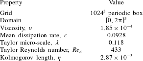
This study makes use of velocity gradient tensors extracted from the Johns Hopkins Turbulence Database numerical simulation of forced isotropic turbulence at a Taylor Reynolds number of 433 (Li et al.
Reference Li, Perlman, Wan, Yang, Burns, Meneveau, Chen, Szalay and Eyink2008) as described by Wan et al. (Reference Wan, Chen, Eyink, Meneveau, Perlman, Burns, Li, Szalay and Hamilton2016). The direct numerical simulation is undertaken on a
 $1024^{3}$
grid using a pseudo-spectral method. The energy is injected to maintain the total energy in the Fourier modes, and also retaining a wavenumber magnitude less than or equal to 2 in each mode. The basic properties of the simulation are summarized in table 3 and a number of other studies have made use of this resource for studying turbulence physics (Wan et al.
Reference Wan, Xiao, Meneveau, Eyink and Chen2010; Lawson & Dawson Reference Lawson and Dawson2015) or for the testing of data post-processing algorithms (Higham, Brevis & Keylock Reference Higham, Brevis and Keylock2016).
Properties of the HIT simulation in the Johns Hopkins database (Li et al. Reference Li, Perlman, Wan, Yang, Burns, Meneveau, Chen, Szalay and Eyink2008).

4 Results: the role of non-normality
4.1 The importance of non-normal effects
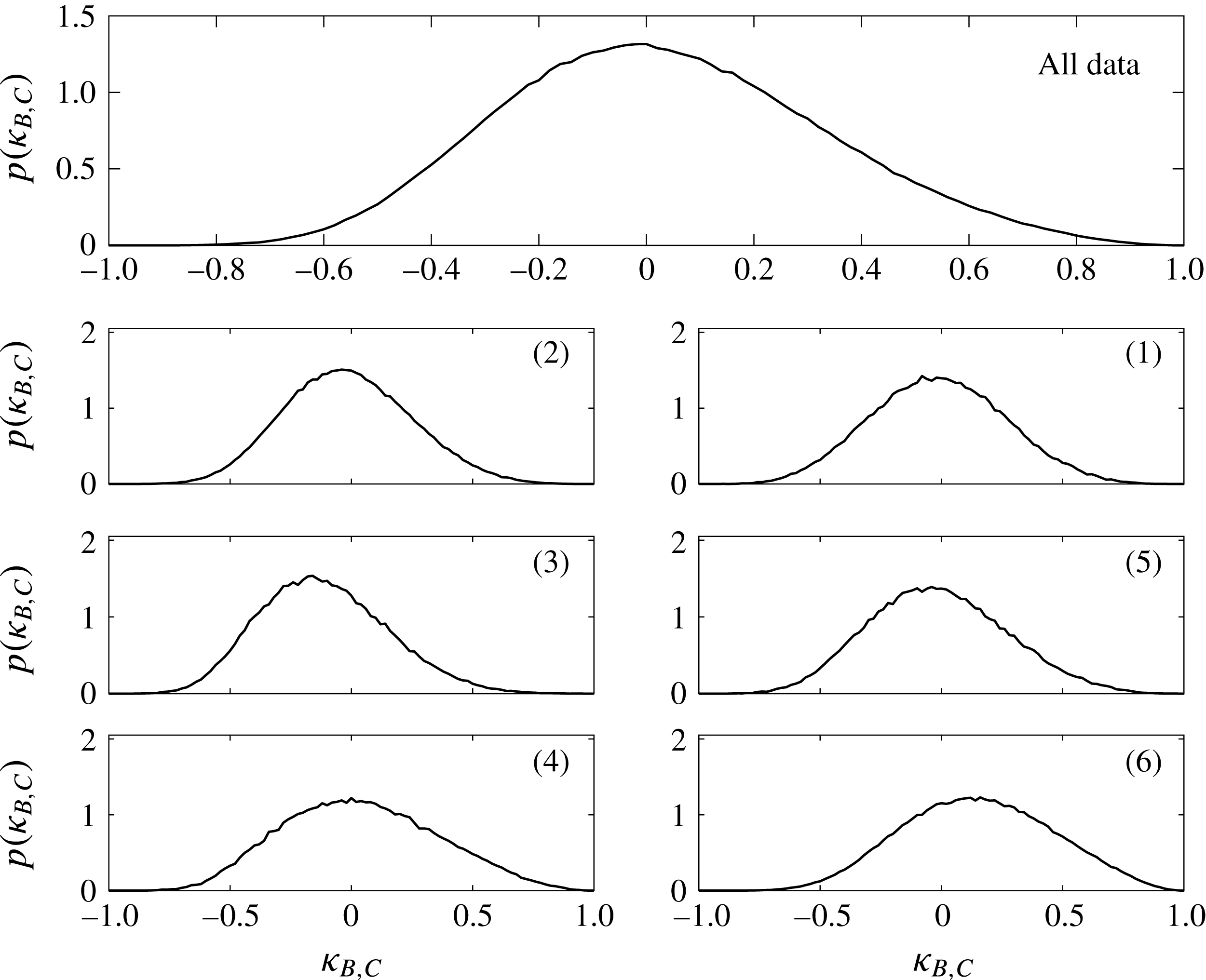
The probability curves for
 $\unicode[STIX]{x1D705}_{B,C}$
, the normalized difference in the Frobenius norms for
 $\unicode[STIX]{x1D63D}$
and
 $\unicode[STIX]{x1D63E}$
, shown for all the data and as a function of the six regions of the
 $\unicode[STIX]{x1D64C}_{A}{-}\unicode[STIX]{x1D64D}_{A}$
diagram in the various panels.

Given
 $\unicode[STIX]{x1D63C}=\unicode[STIX]{x1D63D}+\unicode[STIX]{x1D63E}$
, the first thing to establish is the relative importance of the normal and non-normal tensors; clearly if
 $\unicode[STIX]{x1D63E}$
is small then it is legitimate to approximate the behaviour of
 $\unicode[STIX]{x1D63C}$
with eigenvalue-based formulations. A standardized difference can be used to evaluate this
 $$\begin{eqnarray}\displaystyle \unicode[STIX]{x1D705}_{B,C}=\frac{\Vert \unicode[STIX]{x1D63D}\Vert -\Vert \unicode[STIX]{x1D63E}\Vert }{\Vert \unicode[STIX]{x1D63D}\Vert +\Vert \unicode[STIX]{x1D63E}\Vert }. & & \displaystyle\end{eqnarray}$$
This term is shown in figure 2 and it is clear from the upper panel that the overall mode for the distribution is slightly negative, with a median close to
 $\unicode[STIX]{x1D705}_{B,C}=0$
. Hence, the non-normality is as important to the tensor as the part explained by the eigenvalues. Thus, in HIT, asymmetrical forcings on the tensor as a consequence of non-local effects or viscous effects are an important part of the flow dynamics. When the results in figure 2 are partitioned by the six regions of the
 $\unicode[STIX]{x1D64C}_{A}{-}\unicode[STIX]{x1D64D}_{A}$
diagram, it is clear that for each pair of diagrams in a given
 $\unicode[STIX]{x1D64C}_{A}$
state, it is the left-hand case, with
 $\unicode[STIX]{x1D64D}_{A}<0$
, where the contribution from
 $\Vert \unicode[STIX]{x1D63E}\Vert$
is greater. Region 3 is where
 $\unicode[STIX]{x1D705}_{B,C}$
is most strongly negative and region 6 is where
 $\unicode[STIX]{x1D705}_{B,C}$
is most positive. Thus, an eigenvalue-based description of the flow is particularly effective near the Vieillefosse tail, which is consistent with this being an attractor for the dynamics of the restricted Euler (eigenvalue-based) set of equations for the dynamics of the VGT (Cantwell Reference Cantwell1992).
4.2 The second invariant and non-normality
The distributions for
 $\unicode[STIX]{x1D705}_{Q}^{(\unicode[STIX]{x1D6FA})}$
(solid lines) and
 $\unicode[STIX]{x1D705}_{Q}^{(S)}$
(dot-dashed lines), the normalized differences in the Frobenius norms for
 $\unicode[STIX]{x1D734}_{B}$
and
 $\unicode[STIX]{x1D64E}_{B}$
, respectively, compared to the non-normal term,
 $\unicode[STIX]{x1D64E}_{C}$
. Results are shown for all the data and as a function of the six regions of the
 $\unicode[STIX]{x1D64C}_{A}{-}\unicode[STIX]{x1D64D}_{A}$
diagram. The dashed line in the top panel gives the results for
 $\unicode[STIX]{x1D705}_{Q}^{(\unicode[STIX]{x1D6FA})}$
with the data at
 $\unicode[STIX]{x1D705}_{Q}^{(\unicode[STIX]{x1D6FA})}=-1$
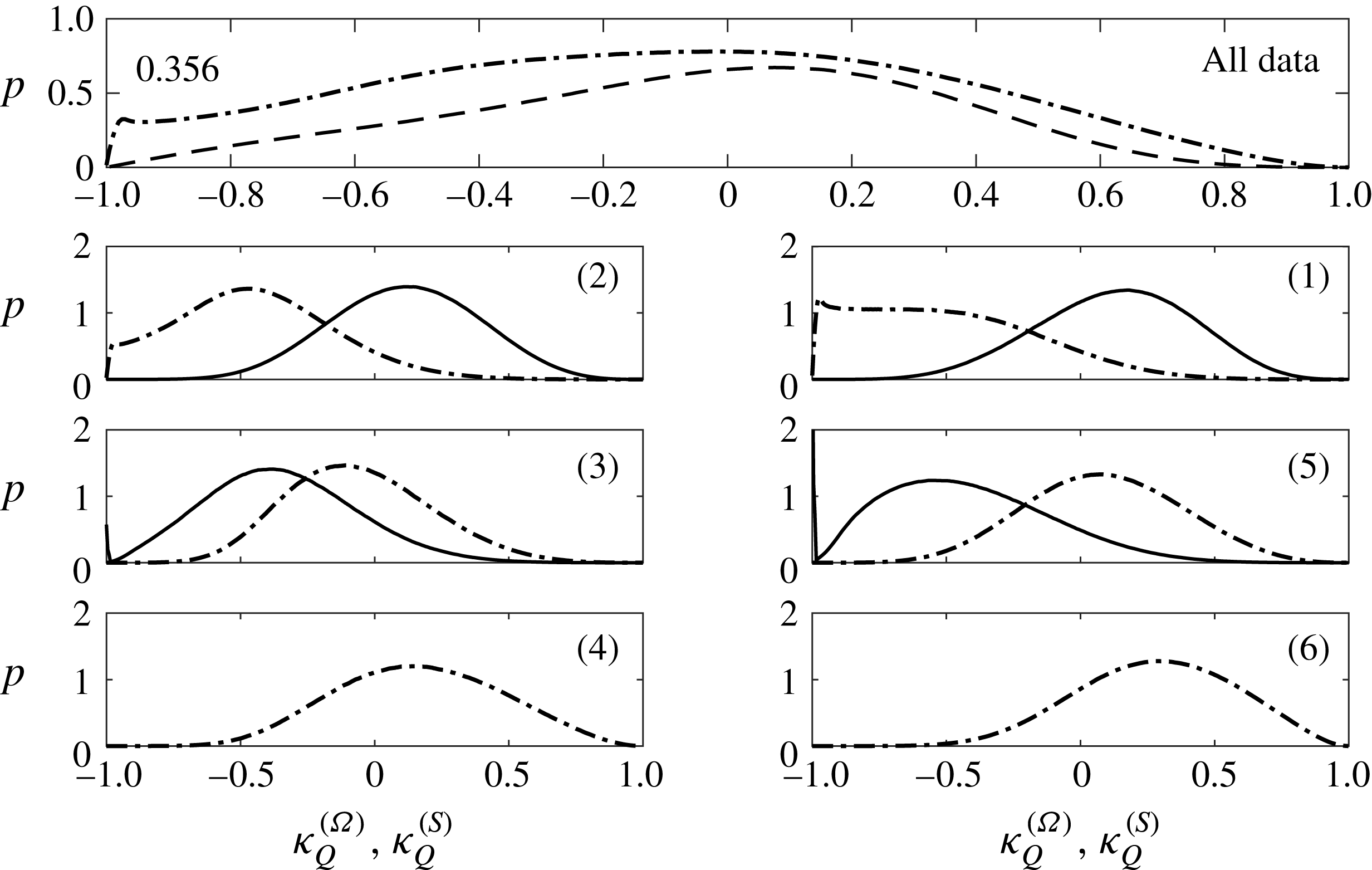
from regions 4 and 6 excluded. Altogether, 35.6 % of values lie at this
 $\unicode[STIX]{x1D705}_{Q}^{(\unicode[STIX]{x1D6FA})}=-1$
limit as stated in this panel.

From (2.11), the components of the second invariant with respect to non-normality are
 $$\begin{eqnarray}\displaystyle & \displaystyle \unicode[STIX]{x1D705}_{Q}^{(\unicode[STIX]{x1D6FA})}=\frac{\Vert \unicode[STIX]{x1D734}_{B}\Vert -\Vert \unicode[STIX]{x1D64E}_{C}\Vert }{\Vert \unicode[STIX]{x1D734}_{B}\Vert +\Vert \unicode[STIX]{x1D64E}_{C}\Vert } & \displaystyle\end{eqnarray}$$
 $$\begin{eqnarray}\displaystyle & \displaystyle \unicode[STIX]{x1D705}_{Q}^{(S)}=\frac{\Vert \unicode[STIX]{x1D64E}_{B}\Vert -\Vert \unicode[STIX]{x1D64E}_{C}\Vert }{\Vert \unicode[STIX]{x1D64E}_{B}\Vert +\Vert \unicode[STIX]{x1D64E}_{C}\Vert }. & \displaystyle\end{eqnarray}$$
Beneath the discriminant function,
 $\unicode[STIX]{x1D705}_{Q}^{(\unicode[STIX]{x1D6FA})}=-1$
by definition and such results are not shown in the panels for regions (4) and (6) in figure 3. While the expected increase in the mean values for
 $\unicode[STIX]{x1D705}_{Q}^{(\unicode[STIX]{x1D6FA})}$
and decrease for
 $\unicode[STIX]{x1D705}_{Q}^{(S)}$
with increasing
 $\unicode[STIX]{x1D64C}_{A}$
is very distinct, the differences as a function of the sign of
 $\unicode[STIX]{x1D64D}_{A}$
are also clearer than in figure 2. For example, while a difference between regions 4 and 6 in their values for
 $\unicode[STIX]{x1D705}_{Q}^{(S)}$
is anticipated from the discussion of figure 2, their respective modes of 0.16 and 0.28 indicate this very clearly. In regions 3 and 5, which is where
 $\unicode[STIX]{x1D6E5}_{L}>0$
and
 $\unicode[STIX]{x1D64C}_{A}<0$
, there is a positive mode for region 5 at
 $\unicode[STIX]{x1D705}_{Q}^{(S)}=0.07$
and a mode of
 $\unicode[STIX]{x1D705}_{Q}^{(S)}=-0.12$
for region 3. Where
 $\unicode[STIX]{x1D64C}_{A}>0$
, the mode in region 1 for
 $\unicode[STIX]{x1D705}_{Q}^{(\unicode[STIX]{x1D6FA})}=0.18$
is more positive than for region 2 (
 $\unicode[STIX]{x1D705}_{Q}^{(\unicode[STIX]{x1D6FA})}=0.12$
), and there is also a stronger tendency for
 $\unicode[STIX]{x1D705}_{Q}^{(S)}\rightarrow -1$
. The importance of non-normal effects in the vortical regions (1 and 2) suggests that a number of properties of vortical structures, such as their topology and alignments, are poorly described by the eigenvalues. Hence, this motivates the additional sections below concerning these aspects of turbulence.
4.3 The third invariant and the four production terms
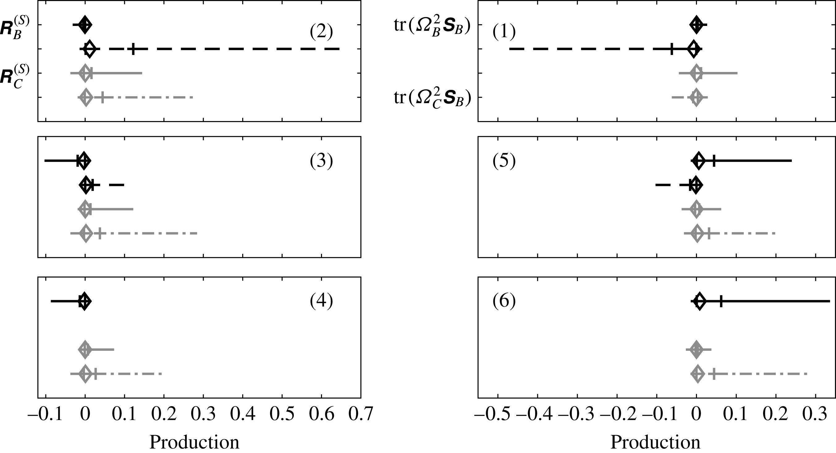
The components of the third invariant are listed and interpreted in table 2 and the probability distributions for the four production terms are synthesized in figure 4, conditioned on the region of the
 $\unicode[STIX]{x1D64C}_{A}{-}\unicode[STIX]{x1D64D}_{A}$
diagram, with values non-dimensionalized by the cube of the Kolmogorov time. As explained in § 2.3,
 $\text{sgn}(\unicode[STIX]{x1D64D}_{B}^{(S)})=\text{sgn}(\unicode[STIX]{x1D64D}_{A})$
and
 $\text{sgn}(\text{tr}(\unicode[STIX]{x1D734}_{B}^{2}\unicode[STIX]{x1D64E}_{B}))=-\text{sgn}(\unicode[STIX]{x1D64D}_{A})$
, while
 $\text{tr}(\unicode[STIX]{x1D734}_{B}^{2}\unicode[STIX]{x1D64E}_{B})=0$
beneath the discriminant function (regions 4 and 6). Thus, the basic properties of these terms (the black lines in figure 4 are known directly from the Schur formalism.
The range of values from the first percentile to the 99th percentile is shown for each of the four production terms conditioned on the region of the
 $\unicode[STIX]{x1D64C}_{A}{-}\unicode[STIX]{x1D64D}_{A}$
diagram (indicated in brackets in each panel). The median value is indicated by a diamond and, where visible, the 10 % and 90 % values are shown by a vertical tick. Values are non-dimensionalized by the Kolmogorov time cubed. The black lines are the normal terms and the grey are the non-normal and interaction terms; which specific term is examined is indicated in the top two panels.

It is clear from figure 4 that both
 $\unicode[STIX]{x1D64C}_{A}>0$
and
 $\unicode[STIX]{x1D6E5}_{L}>0$
are relevant to classifying the flow behaviour, justifying the separation of the
 $\unicode[STIX]{x1D64C}_{A}{-}\unicode[STIX]{x1D64D}_{A}$
diagram into six regions. First,
 $\text{tr}(\unicode[STIX]{x1D734}_{B}^{2}\unicode[STIX]{x1D64E}_{B})$
does not occur for
 $\unicode[STIX]{x1D6E5}_{L}<0$
as just described and, second, all other terms exhibit a clearer difference between positive and negative
 $\unicode[STIX]{x1D64C}_{A}$
states than positive and negative
 $\unicode[STIX]{x1D6E5}_{L}$
states. For example, in regions 5 and 6, the positive tail of the distributions for both
 $\unicode[STIX]{x1D64D}_{B}^{(S)}$
and
 $\text{tr}(\unicode[STIX]{x1D734}_{C}^{2}\unicode[STIX]{x1D64E}_{B})$
is clear. However, in region 1, the latter changes sign and the former collapses dramatically. In addition,
 $\unicode[STIX]{x1D64D}_{C}^{(S)}$
becomes more positively skewed and
 $\text{tr}(\unicode[STIX]{x1D734}_{B}^{2}\unicode[STIX]{x1D64E}_{B})$
more negatively skewed. That there is little difference between regions 5 and 6 for three of the terms, means that the emergence of negative contributions from
 $\text{tr}(\unicode[STIX]{x1D734}_{B}^{2}\unicode[STIX]{x1D64E}_{B})$
in region 5 is the sole major difference to the dynamics.
In regions 3 and 4, the non-normal and interaction production terms are broadly similar to regions 5 and 6 but the normal terms are opposite in sign and the tail to the normal strain production term is much shorter. Regions 1 and 2 are qualitatively different both to each other and to the other regions. Clearly, normal enstrophy production dominates in these two regions and is necessarily opposite in sign between them. In addition, non-normal production,
 $\unicode[STIX]{x1D64D}_{C}^{(S)}$
is more positively skewed in these two regions than elsewhere. However, while the interaction term is positively skewed in other regions, in region 1 it exhibits a weak negative skew. As a consequence of the sign for
 $\text{tr}(\unicode[STIX]{x1D734}_{B}^{2}\unicode[STIX]{x1D64E}_{B})$
, positive production in region 1 comes from the non-normal term. Hence, positive values for
 $\unicode[STIX]{x1D64D}_{A}$
, in region 1 are driven by positive non-normal production and negative normal enstrophy production rather than positive normal production, as is the case in regions 5 and 6.
A typical Lagrangian trajectory is from region 2 to region 1, where there is a change from two negative eigenvalues for
 $\unicode[STIX]{x1D64D}_{B}^{(S)}$
(rods) to one (discs). However, the small magnitude for
 $\unicode[STIX]{x1D64D}_{B}^{(S)}$
means that the non-normal and interaction terms will be important for establishing the values for
 $\unicode[STIX]{x1D64D}_{A}^{(S)}$
. This is explored in § 5.
4.4 Joint behaviour of the four production terms
Joint probability distributions for
 $\unicode[STIX]{x1D64D}_{B}^{(S)}$
and the combined non-normal and interaction terms conditioned on the region of the
 $\unicode[STIX]{x1D64C}_{A}{-}\unicode[STIX]{x1D64D}_{A}$
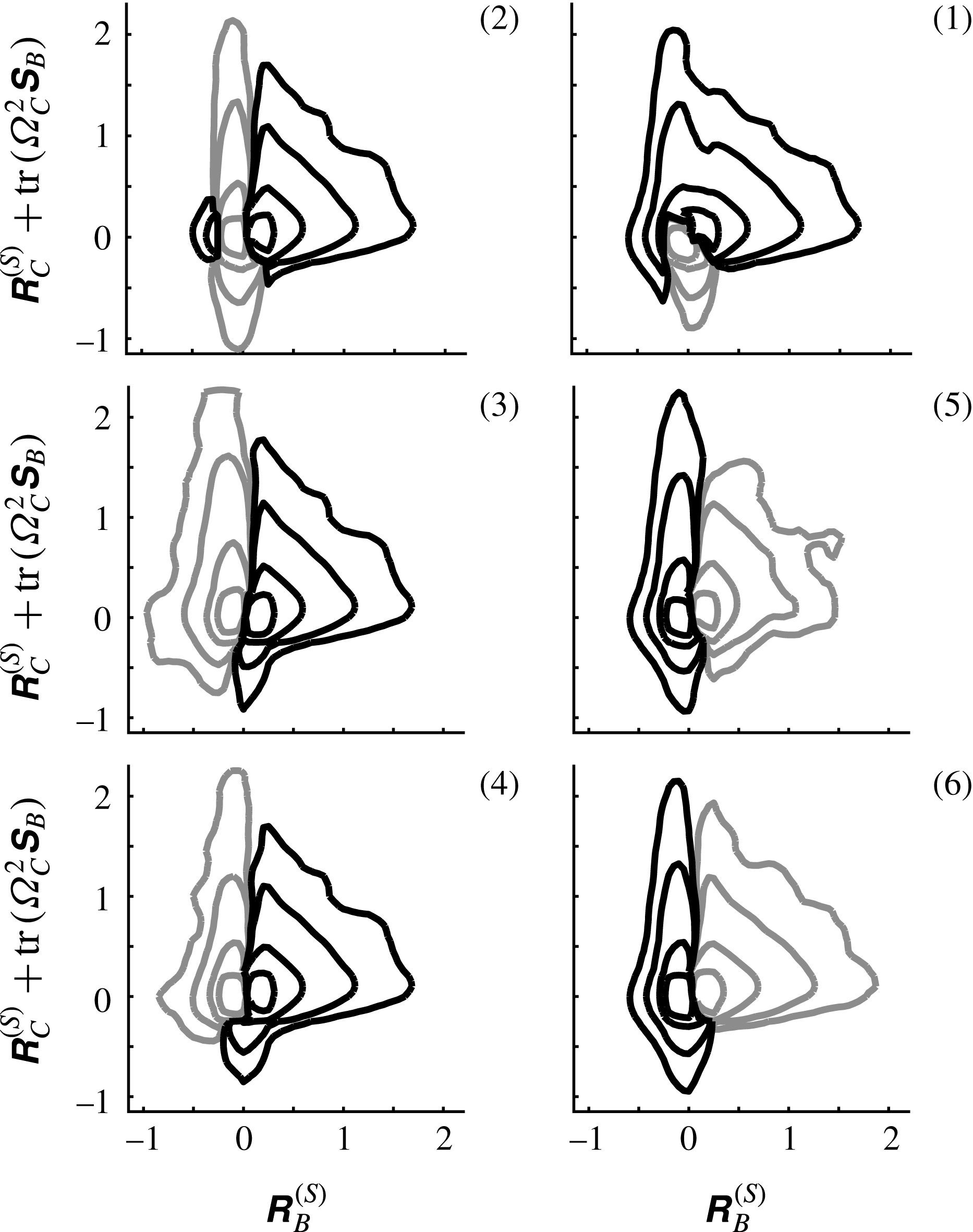
diagram, and written as the difference between the distribution in this region and the overall distributions function. Positive values indicate an excess for this region and have the lighter probability contours. Contours are approximately logarithmically distributed:
 $\pm 2\times 10^{-3}$
,
 $\pm 1\times 10^{-2}$
,
 $\pm 1\times 10^{-1}$
,
 $\pm 1\times 10^{0}$
.

Joint probability distributions for
 $\text{tr}(\unicode[STIX]{x1D734}_{B}^{2}\unicode[STIX]{x1D64E}_{B})$
and the combined non-normal and interaction terms conditioned on the region of the
 $\unicode[STIX]{x1D64C}_{A}{-}\unicode[STIX]{x1D64D}_{A}$
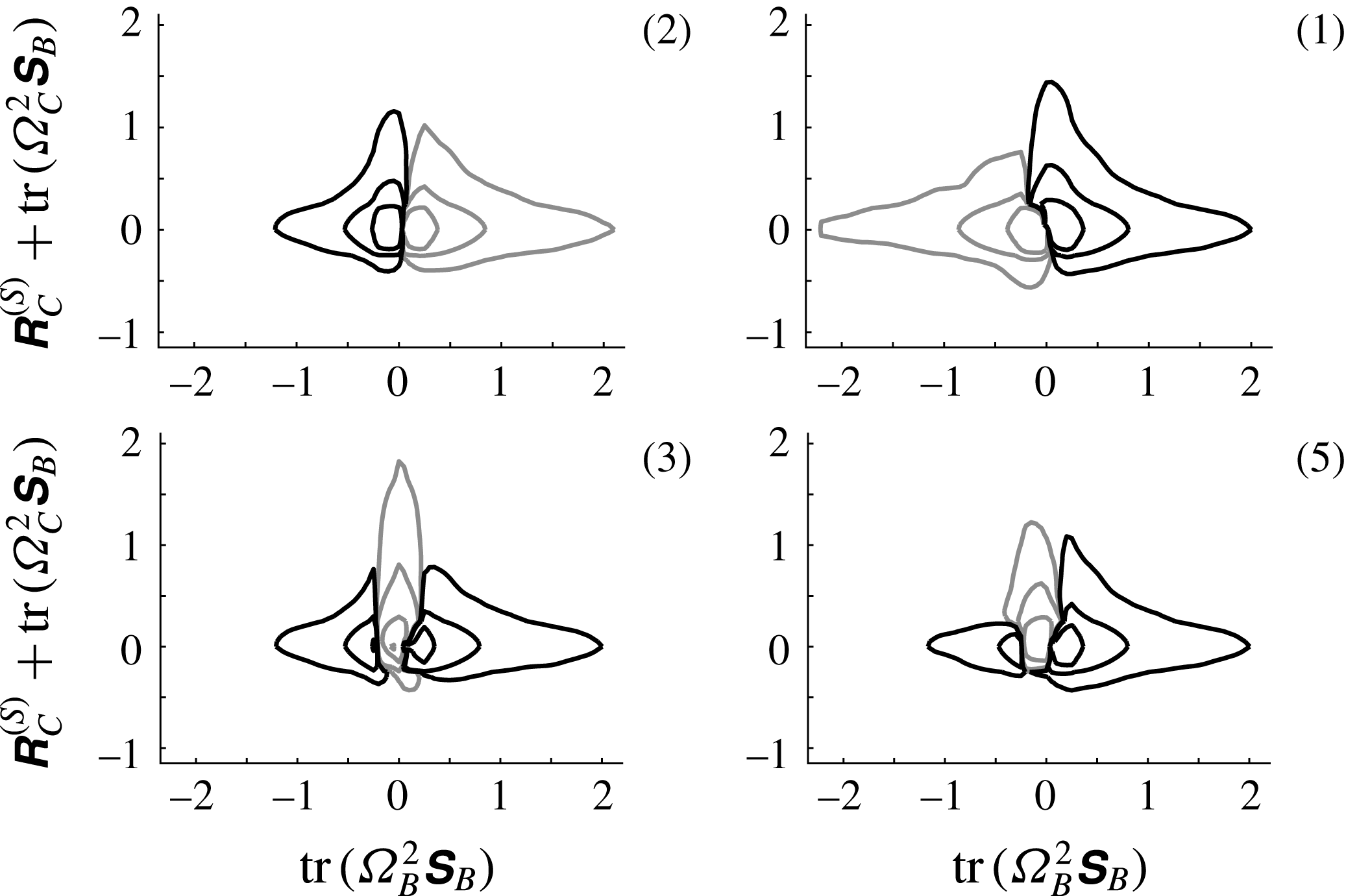
diagram, and written as the difference between the distribution in this region and the overall distributions function. Positive values indicate an excess for this region and have the lighter probability contours. Contours are logarithmically distributed:
 $\pm 1\times 10^{-2}$
,
 $\pm 1\times 10^{-1}$
,
 $\pm 1\times 10^{0}$
.

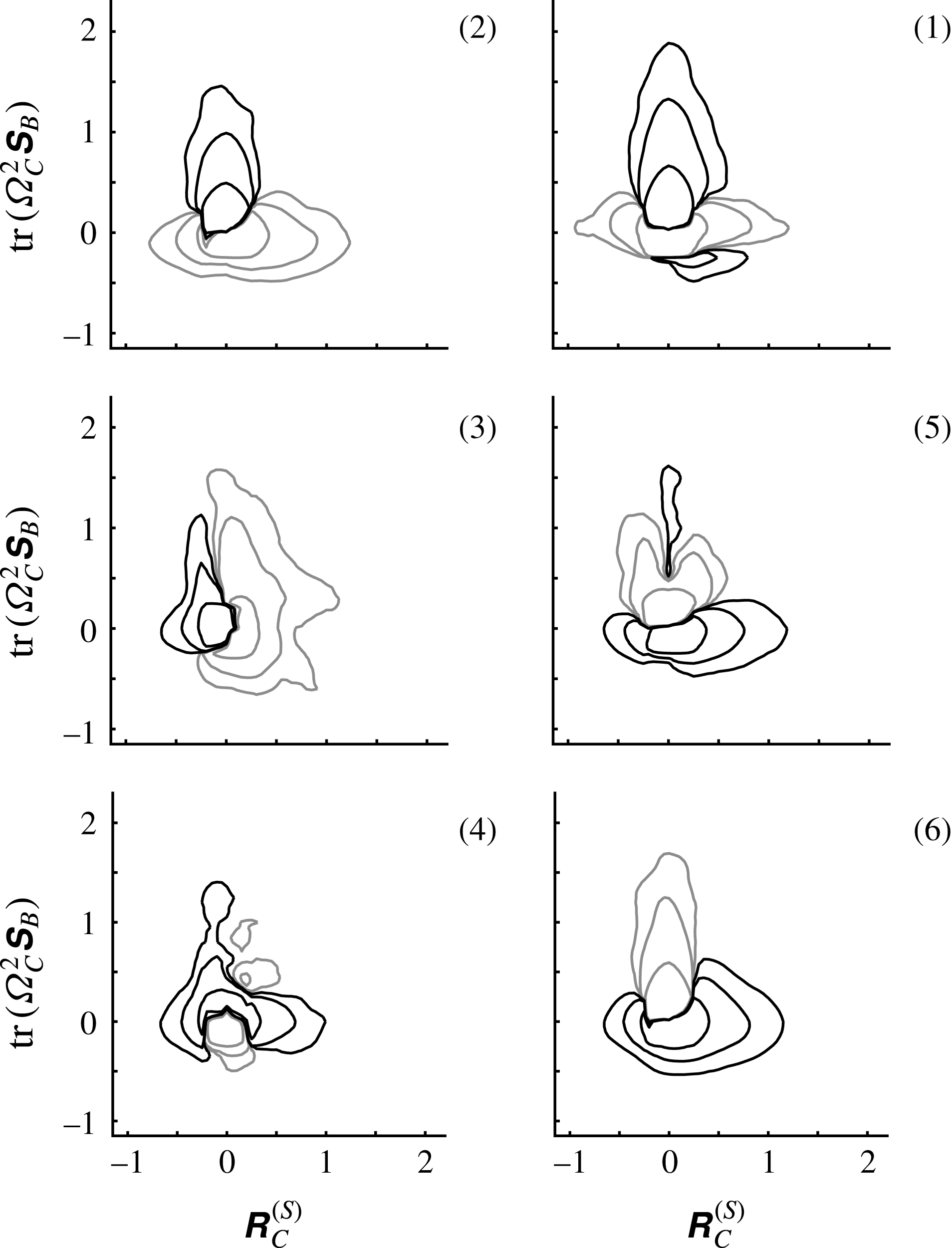
Further information on the structure of the production terms can be gleaned from their joint behaviour. Hence, in this section normal strain production is compared to the combined influence of the non-normal and interaction terms (figure 5), normal enstrophy production is compared to the combined influence of the non-normal and interaction terms (figure 6) and then the joint behaviour of the latter two terms is studied (figure 7). Again, each term is non-dimensionalized by the cube of the Kolmogorov time. Each panel in these three figures displays the results for each region of the
 $\unicode[STIX]{x1D64C}_{A}{-}\unicode[STIX]{x1D64D}_{A}$
diagram as a difference from the overall joint probability distribution function (PDF) for all regions combined, with lighter (darker) contours highlighting an excess (deficit) to the distribution function for this region.
There is a basic pattern to these joint distributions anticipated from the signs for
 $\unicode[STIX]{x1D64D}_{B}^{(S)}$
and
 $\text{tr}(\unicode[STIX]{x1D734}_{B}^{2}\unicode[STIX]{x1D64E}_{B})$
on each half of the
 $\unicode[STIX]{x1D64C}_{A}{-}\unicode[STIX]{x1D64D}_{A}$
diagram, with positive strain production and negative enstrophy production occurring on the right-hand side and the opposite case seen on the left. However, the sign of
 $\unicode[STIX]{x1D64C}_{A}$
is important for the strength to which this tendency is expressed. The anticipated pattern is seen for strain dominant regions where
 $\unicode[STIX]{x1D64C}_{A}<0$
in figure 5 and for enstrophy dominated regions where
 $\unicode[STIX]{x1D64C}_{A}>0$
in figure 6. For strain dominated regions in figure 6, the combined effect of the non-normal and interaction production terms is essentially positive. For enstrophy dominated regions in figure 5, region 2 exhibits an excess for either sign of the combined term, while for region 1 the excess is clearly for negative values of the combined term. It is clear from the results in figure 5 for regions 5 and 6 why strain production is highest around the Vieillefosse tail: a strong local excess for positive normal strain production is reinforced by positive contributions from the non-normal and interaction production terms.
Disaggregating the behaviour of this term, figure 7 shows that it is the non-normal term that dominates in both regions 1 and 2, and that this can take either sign. Region 6 is very much limited to positive excess contributions from the interaction term, and it is true that it is this term that results in the positive bias for contributions from region 5, although larger magnitude values arise for the non-normal term, reflecting the status of region 5 as intermediary between regions 1 and 6. Region 3 is the case where a largely positive response is a consequence of a jointly positive contribution from both terms – this is the region where reducing the effect to one or other of the marginal distributions shown in figure 7 is inadequate. Positive contributions from region 4 are a preferential consequence of positive values for
 $\unicode[STIX]{x1D64D}_{C}^{(S)}$
, irrespective of the sign for
 $\text{tr}(\unicode[STIX]{x1D734}_{C}^{2}\unicode[STIX]{x1D64E}_{B})$
. Thus, future models for the VGT dynamics in the spirit of recent approaches (Wilczek & Meneveau Reference Wilczek and Meneveau2014; Johnson & Meneveau Reference Johnson and Meneveau2016) but including information from this study, may wish to consider stochastic, small-scale forcings from the non-normal contributions in accord with the marginal and joint distributions presented here.
Joint probability distributions for
 $\unicode[STIX]{x1D64D}_{C}^{(S)}$
and
 $\text{tr}(\unicode[STIX]{x1D734}_{C}^{2}\unicode[STIX]{x1D64E}_{B})$
conditioned on the region of the
 $\unicode[STIX]{x1D64C}_{A}{-}\unicode[STIX]{x1D64D}_{A}$
diagram, and written as the difference between the distribution in this region and the overall distributions function. Positive values indicate an excess for this region and have the lighter probability contours. Contours are approximately logarithmically distributed:
 $\pm 2.5\times 10^{-3}$
,
 $\pm 1\times 10^{-2}$
,
 $\pm 1\times 10^{-1}$
.

5 Results: The second eigenvalue of the strain rate tensor for
$\unicode[STIX]{x1D63C}$

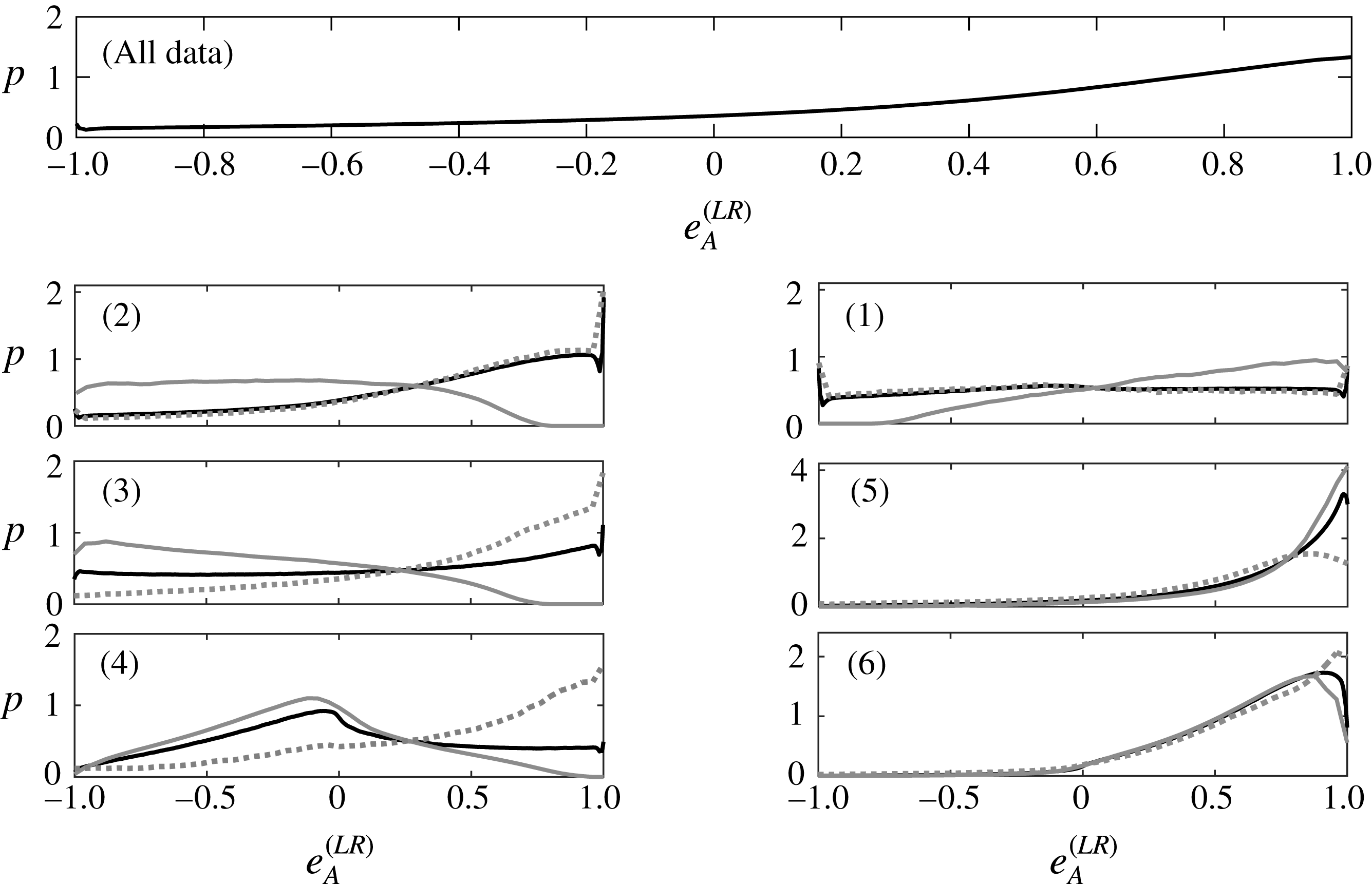
Probability distributions for
 $e_{A}^{(LR)}$
for all the data (a) and then by each region of the
 $\unicode[STIX]{x1D64C}_{A}{-}\unicode[STIX]{x1D64D}_{A}$
diagram (black lines). Results are also shown conditioned on the sign of
 $\unicode[STIX]{x1D705}_{Q}^{(S)}$
, with
 $\unicode[STIX]{x1D705}_{Q}^{(S)}>0$
as a grey solid line and
 $\unicode[STIX]{x1D705}_{Q}^{(S)}<0$
as a grey dotted line.

The well-known tendency for HIT to form disc-like structures is shown in figure 8(a) using the Lund and Rogers normalization,
 $e_{A}^{(LR)}$
given in (2.22). Sub-dividing the results by region of the
 $\unicode[STIX]{x1D64C}_{A}{-}\unicode[STIX]{x1D64D}_{A}$
diagram shows that this tendency is driven by regions 2, 5 and 6. However, given that positive strain production,
 $-\text{det}(\unicode[STIX]{x1D64E}_{A})>0$
means there are two positive strain eigenvalues, inducing disc-like structures in an incompressible flow, in regions 1, 5 and 6, the unusual extent of non-normal production in region 1, already highlighted, must explain this weak contribution to this tendency from region 1. When looking at
 $e_{A}^{(LR)}$
conditioned on the sign of
 $\unicode[STIX]{x1D705}_{Q}^{(S)}$
(the grey lines in figure 8), where
 $\unicode[STIX]{x1D705}_{Q}^{(S)}>0$
(solid grey lines) the anticipated behaviour of a tendency for
 $e_{A}^{(LR)}\rightarrow +1$
in region 1 and
 $e_{A}^{(LR)}\rightarrow -1$
in region 2 is seen. However, the grey dashed lines, representing
 $\unicode[STIX]{x1D705}_{Q}^{(S)}<0$
states arise much more frequently (
 ${\sim}90\,\%$
of cases), meaning they drive the overall pattern in figure 8. It is these data that exhibit the strong
 $e_{A}^{(LR)}\rightarrow +1$
tendency in region 2, and a flat distribution function in region 1.
Consequently, the reason for the observed behaviour is that the non-normal contribution to the strain tensor is significant and produces a very different behaviour to that driven by the eigenvalues. Given that it is in regions 1 and 2 where enstrophy exceeds strain and, according to the
 $Q$
-criterion (Hunt et al.
Reference Hunt, Wray and Moin1988; Dubief & Delcayre Reference Dubief and Delcayre2000), is where there is a coherence to vortical motion, non-normality is crucial for the evolution of coherent, vortical disc-like structures. As contributions from the non-normality tensor,
 $\unicode[STIX]{x1D63E}$
, do not feature in the restricted Euler formulation of the VGT dynamics, anisotropic contributions from the pressure Hessian and viscous effects must be extremely important for this aspect of the topology. From table 1, region 2 is frequented more than twice as often as region 1 (26.5 %–11.1 %), which also helps explain the strong tendency for
 $e_{A}^{(LR)}\rightarrow 1$
seen in the top-most panel.
Figure 3 shows that
 $\unicode[STIX]{x1D705}_{Q}^{(S)}>0$
occurs for 39.4 %, 68.6 %, 60.6 % and 82.2 % of occurrences in regions 3 to 6, respectively (i.e. the normal contributions to strain are larger in regions 4 and 6). In figure 8 it is region 5 where
 $\unicode[STIX]{x1D705}_{Q}^{(S)}>0$
has the strongest tendency to produce values at
 $e_{A}^{(LR)}=1$
, while everywhere but region 1, one finds that
 $\unicode[STIX]{x1D705}_{Q}^{(S)}<0$
preferentially leads to positive values for
 $e_{A}^{(LR)}$
. The complex case is region 4, where the normal contribution to the strain is strongly dominant, but has a mode at
 $e_{A}^{(LR)}=-0.08$
, indicating that here the preferred state is close to isotropy (the ‘blob’ in the terminology of Kuo & Corrsin (Reference Kuo and Corrsin1972)); any tendency to form disc-like structures is a consequence of the non-normal dominant cases in this region.
5.1 The disaggregation of the Lund and Rogers normalization of the strain rate tensor
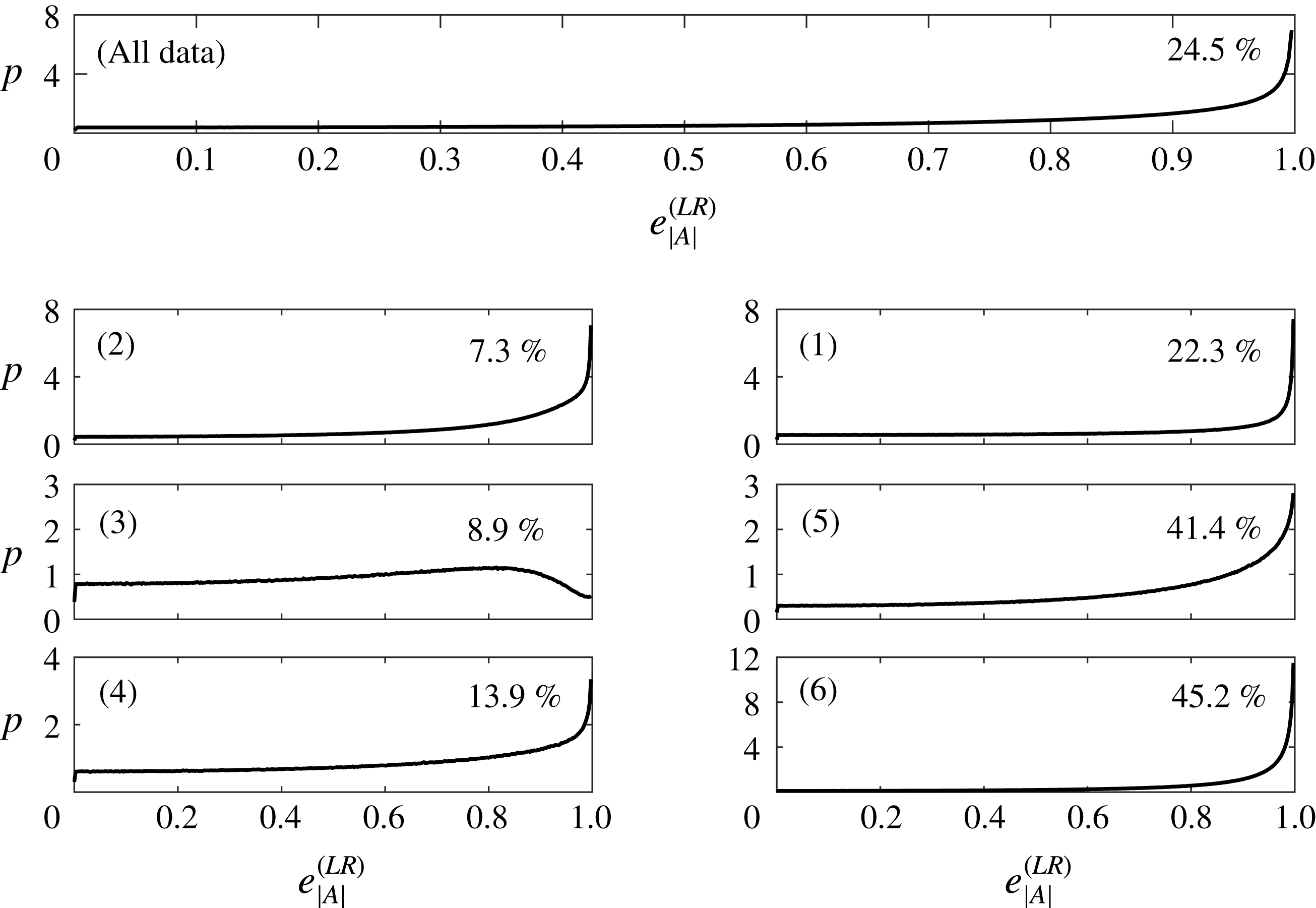
Distribution functions for
 $e_{|A|}^{(LR)}$
are shown for all the data and by region of the
 $\unicode[STIX]{x1D64C}_{A}{-}\unicode[STIX]{x1D64D}_{A}$
diagram. Values are shown with a continuous line for
 $0\leqslant e_{|A|}^{(LR)}<1$
. The stated value in each panel is the percentage of values for which
 $e_{|A|}^{(LR)}=1$
, i.e. this is where none of the three terms contributing to the value for
 $e_{A}^{(LR)}$
have a sign different to that for
 $e_{A}^{(LR)}$
.

It was established in § 2.5 that
 $e_{A}^{(LR)}=e_{B|A}^{(LR)}+e_{C|A}^{(LR)}+e_{C,B|A}^{(LR)}$
and it is the component terms on the right-hand side that we investigate in this sub-section. However,
 $$\begin{eqnarray}e_{|A|}^{(LR)}=\left|\frac{e_{A}^{(LR)}}{|e_{B|A}^{(LR)}|+|e_{C|A}^{(LR)}|+|e_{C,B|A}^{(LR)}|}\right|,\end{eqnarray}$$
may be used to gain an insight into how common it is for some of these component terms to have the opposite sign to
 $e_{|A|}^{(LR)}$
and the relative magnitude of such effects as a function of
 $\unicode[STIX]{x1D64C}_{A}$
and
 $\unicode[STIX]{x1D64D}_{A}$
. Given the tendency in HIT for
 $e_{A}^{(LR)}\rightarrow 1$
and that, as explained in § 2.5,
 $\text{sgn}(e_{B|A}^{(LR)})=\text{sgn}(\unicode[STIX]{x1D64D}_{A})$
, it is expected that
 $e_{|A|}^{(LR)}\neq 1$
more often in regions 2, 3, and 4, where
 $\unicode[STIX]{x1D64D}_{A}<0$
. Figure 9 shows this is the case, particularly where
 $\unicode[STIX]{x1D6E5}_{L}>0$
in regions 2 and 3 (and to a certain extent also in region 1 where
 $\unicode[STIX]{x1D64D}_{A}>0$
but
 $\unicode[STIX]{x1D64C}_{A}>0$
). Indeed, with the exception of region 1, the overall result in the upper panel that approximately 25 % of tensors in HIT have
 $e_{|A|}^{(LR)}=1$
is not representative of the behaviour of the individual regions.
It follows from these results that the joint distribution function for the normal term,
 $e_{B|A}^{(LR)}$
, and the combined non-normal and interaction terms,
 $e_{C|A}^{(LR)}+e_{C,B|A}^{(LR)}$
, should exhibit the strongest probability gradient near the frontier
 $e_{B|A}^{(LR)}+e_{C|A}^{(LR)}+e_{C,B|A}^{(LR)}=1$
and where both
 $e_{B|A}^{(LR)}$
and
 $(e_{C|A}^{(LR)}+e_{C,B|A}^{(LR)})$
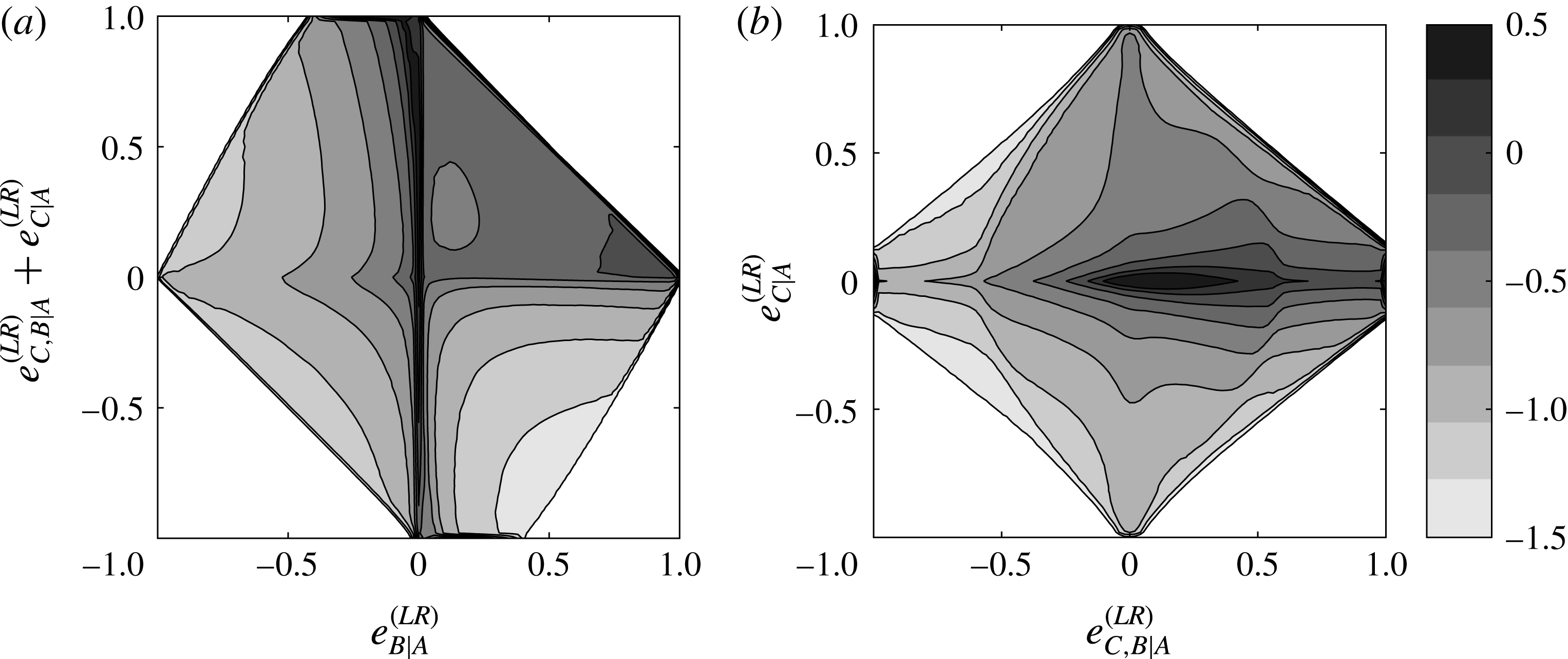
are positive. Positive values for
 $e_{B|A}^{(LR)}$
mean the tensor is in region 1, 5 or 6. Such a frontier is clear in figure 10(a).
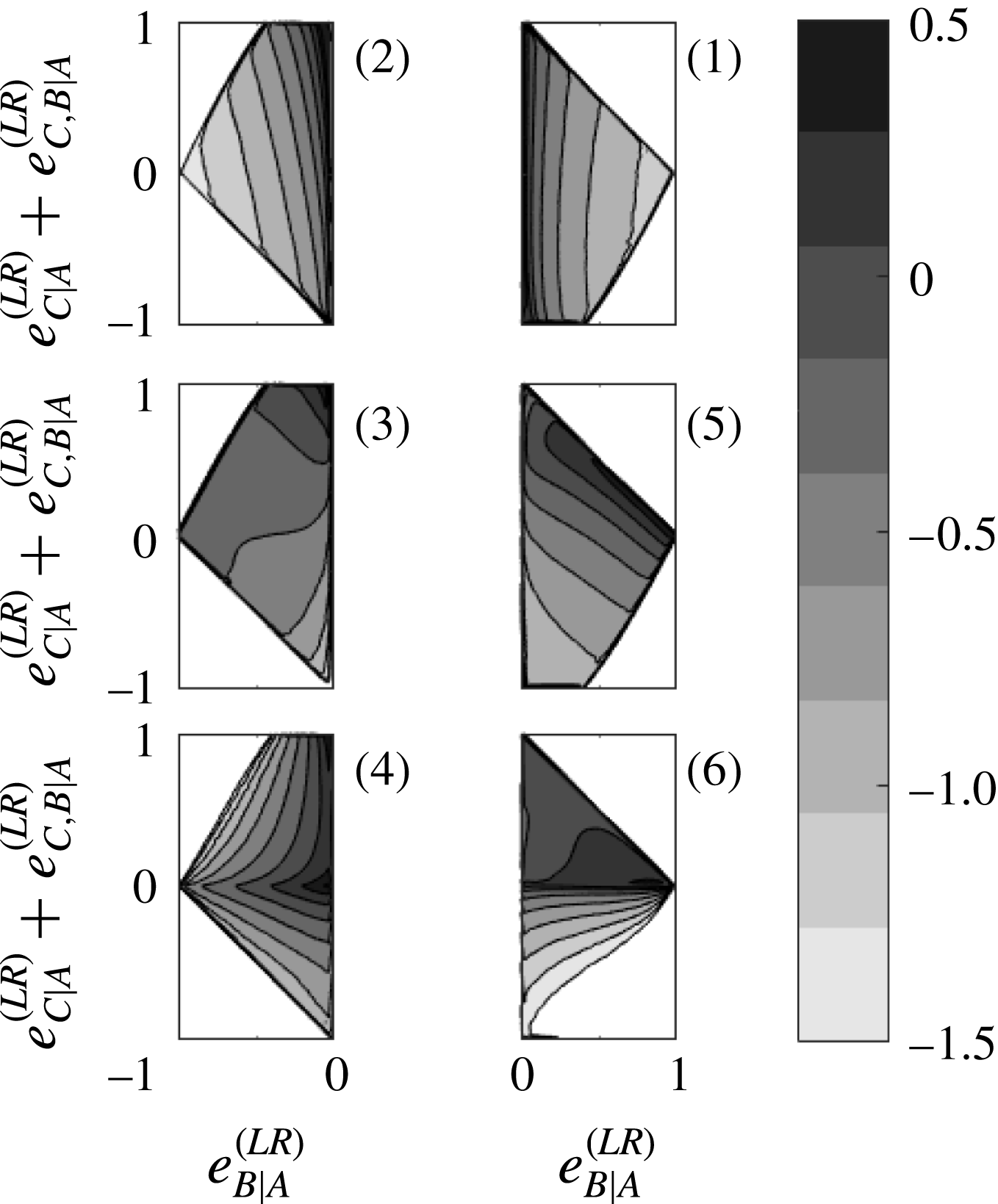
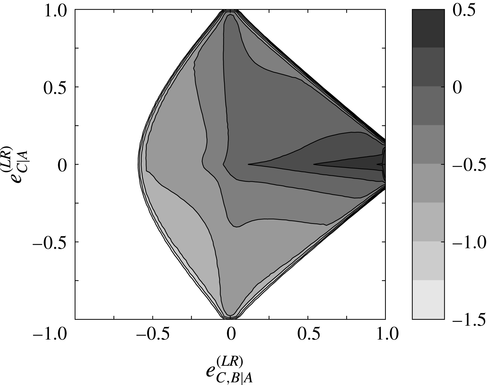
Joint distribution functions for
 $e_{B|A}^{(LR)}$
and
 $e_{C|A}^{(LR)}+e_{C,B|A}^{(LR)}$
(a) as well as
 $e_{C|A}^{(LR)}$
and
 $e_{C,B|A}^{(LR)}$
(b). Contours are on a
 $\text{log}_{10}$
scale.

In this same panel, where
 $e_{B|A}^{(LR)}<0$
, the combined behaviour of the non-normal and interaction terms behaves with some degree of symmetry about
 $e_{C|A}^{(LR)}+e_{C,B|A}^{(LR)}=0$
, although with a bias towards positive values as might be expected from the global result of a tendency for
 $e_{A}^{(LR)}\rightarrow 1$
. Therefore, positive values for
 $e_{A}^{(LR)}$
may readily arise even when
 $e_{B|A}^{(LR)}<0$
as a consequence of the action of the non-normal and interaction terms as shown in a less direct fashion from the conditioning on
 $\unicode[STIX]{x1D705}_{Q}^{(S)}$
in figure 8.
For positive
 $e_{B|A}^{(LR)}$
negative values for the
 $e_{C|A}^{(LR)}+e_{C,B|A}^{(LR)}$
term are highly improbable, except at the limit,
 $e_{C|A}^{(LR)}+e_{C,B|A}^{(LR)}=-1$
, for weakly positive values for
 $e_{B|A}^{(LR)}$
. From an inspection of figure 10(b), the
 $e_{C|A}^{(LR)}+e_{C,B|A}^{(LR)}=-1$
state arises preferentially where
 $e_{C|A}^{(LR)}=0$
,
 $e_{C,B|A}^{(LR)}=-1$
, showing the importance of the interaction term for generating rod-like structures. That there is a good degree of symmetry to figure 10(b) about
 $e_{C|A}^{(LR)}=0$
indicates that the sign of
 $e_{C|A}^{(LR)}$
is not predicted by
 $e_{C,B|A}^{(LR)}$
. That the centre-of-mass of the distribution resides to the right side of figure 10(b) shows that the interaction term is driving the positive bias in values for
 $e_{A}^{(LR)}$
overall.
Joint distribution functions for
 $e_{B|A}^{(LR)}$
and
 $e_{C|A}^{(LR)}+e_{C,B|A}^{(LR)}$
using the same logarithmic scaling for the contours as adopted in figure 10, with results sub-divided by the six regions of the
 $\unicode[STIX]{x1D64C}_{A}{-}\unicode[STIX]{x1D64D}_{A}$
diagram defined in table 1.

5.2 Results conditioned on
$\unicode[STIX]{x1D64C}_{A}{-}\unicode[STIX]{x1D64D}_{A}$
states

Having presented the general pattern for how the normal, non-normal and interaction terms are coupled in figure 10(a), results conditioned on the different regions of
 $\unicode[STIX]{x1D64C}_{A}{-}\unicode[STIX]{x1D64D}_{A}$
space are shown in figure 11. Thus, the strong probability frontier in figure 10(a) and the secondary mode near
 $e_{B|A}^{(LR)}=1$
arise due to the behaviour in regions 5 and 6, respectively. In contrast
 $e_{B|A}^{(LR)}=-1$
is more common in region 3 than region 4, and greater relative importance of the non-normal and interaction terms occurs in region 4 compared to region 6, as
 $e_{B|A}^{(LR)}\rightarrow 0$
in region 4. The
 $\unicode[STIX]{x1D64C}_{A}{-}\unicode[STIX]{x1D64D}_{A}$
diagram exhibits a concentration of values in regions 2 and 6 as shown in table 1. Figure 11 shows that the tendency to disc-like structures in region 6 is driven firstly by
 $e_{B|A}^{(LR)}$
and then by the combined interaction of all terms that defines the strong frontier. In contrast, while region 2 contributes effectively to this tendency to form disc-like structures, figure 11 shows that this result is driven by
 $e_{C,B|A}^{(LR)}$
or
 $e_{C|A}^{(LR)}$
. It is clear from figure 12 that, by and large, the interaction term is dominating this tendency to form disc-like structures.
The joint distribution function for
 $e_{C|A}^{(LR)}$
and
 $e_{C,B|A}^{(LR)}$
for region 2 of the
 $\unicode[STIX]{x1D64C}_{A}{-}\unicode[STIX]{x1D64D}_{A}$
diagram using the same logarithmic scaling for the contours as adopted in figure 10.

In summary, the well-known tendency for
 $e_{A}^{(LR)}\rightarrow 1$
cannot be explained merely by the tendency for turbulence to reside preferentially in positive
 $\unicode[STIX]{x1D64D}_{A}$
states as this bias is only 54.6 : 45.4 (table 1). However, with region 2 replacing region 1 as a contributor to such a topology as a consequence of the action of non-normality, such a ratio becomes 70 : 30. Each region of the
 $\unicode[STIX]{x1D64C}_{A}{-}\unicode[STIX]{x1D64D}_{A}$
diagram has a novel signature, with the normal straining,
 $e_{B|A}^{(LR)}$
, of greatest importance in region 5 and 6, and of limited importance in the vortical regions. Region 1 acts counter to the general tendency for the formation of disc-like structures despite the fact that
 $\unicode[STIX]{x1D64D}_{A}>0$
, because of the importance of the non-normal and interaction terms. In general, in this region contributions from the non-normal term are positive, while the interaction term is negative. Hence, the smaller-scale anisotropies induced by viscous and non-local effects have a profound impact on the topology of flow structures in the regions where enstrophy dominates total strain.
6 Results: vorticity vector and strain eigenvector alignments
6.1 The existing relations for
$\unicode[STIX]{x1D63C}$

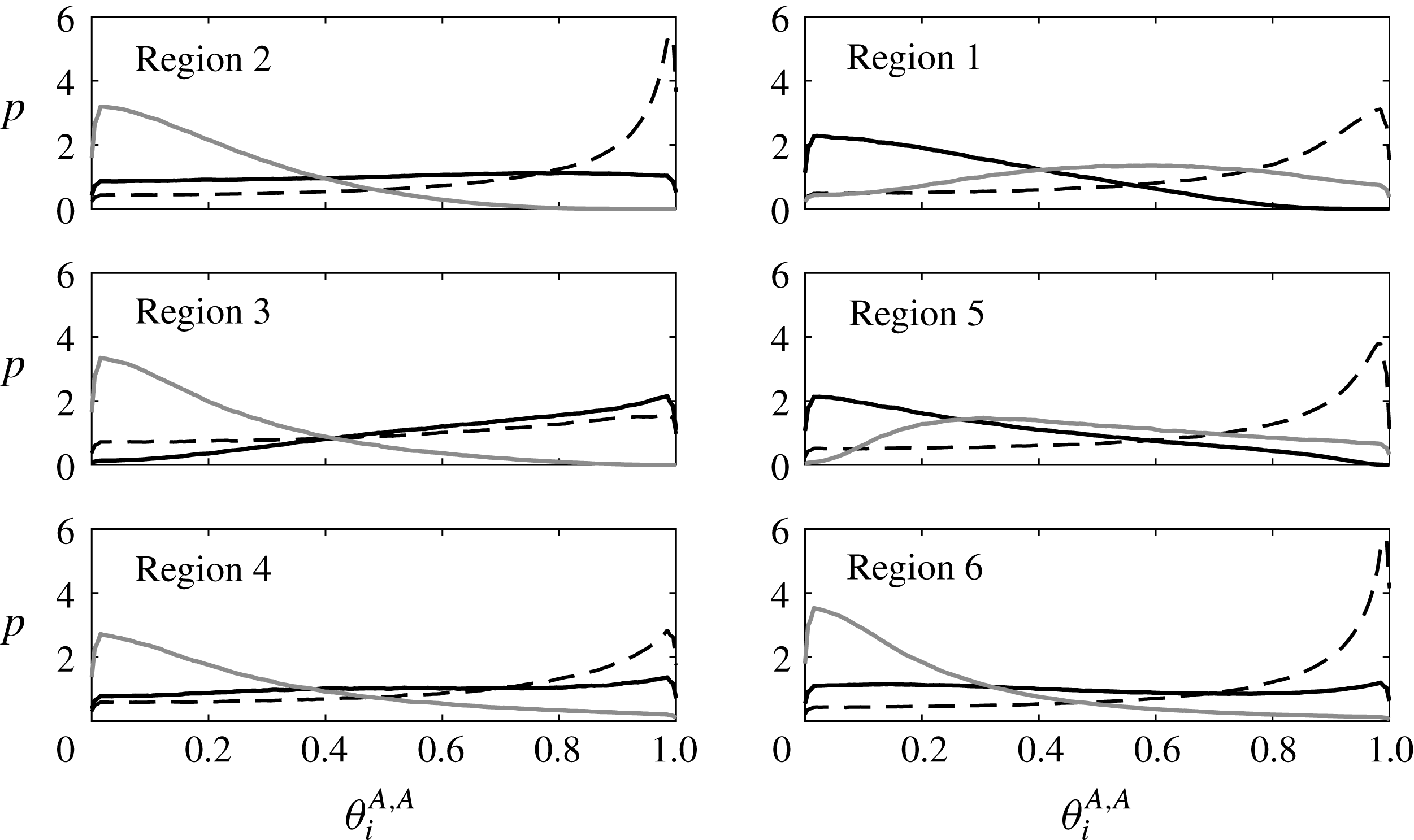
Distribution functions for the alignments,
 $\unicode[STIX]{x1D703}_{i}^{A,A}$
between the vorticity vector and the strain eigenvectors for
 $\unicode[STIX]{x1D63C}$
. The black solid line is for
 $i=1$
, the dashed line is for
 $i=2$
and the grey line is for
 $i=3$
.

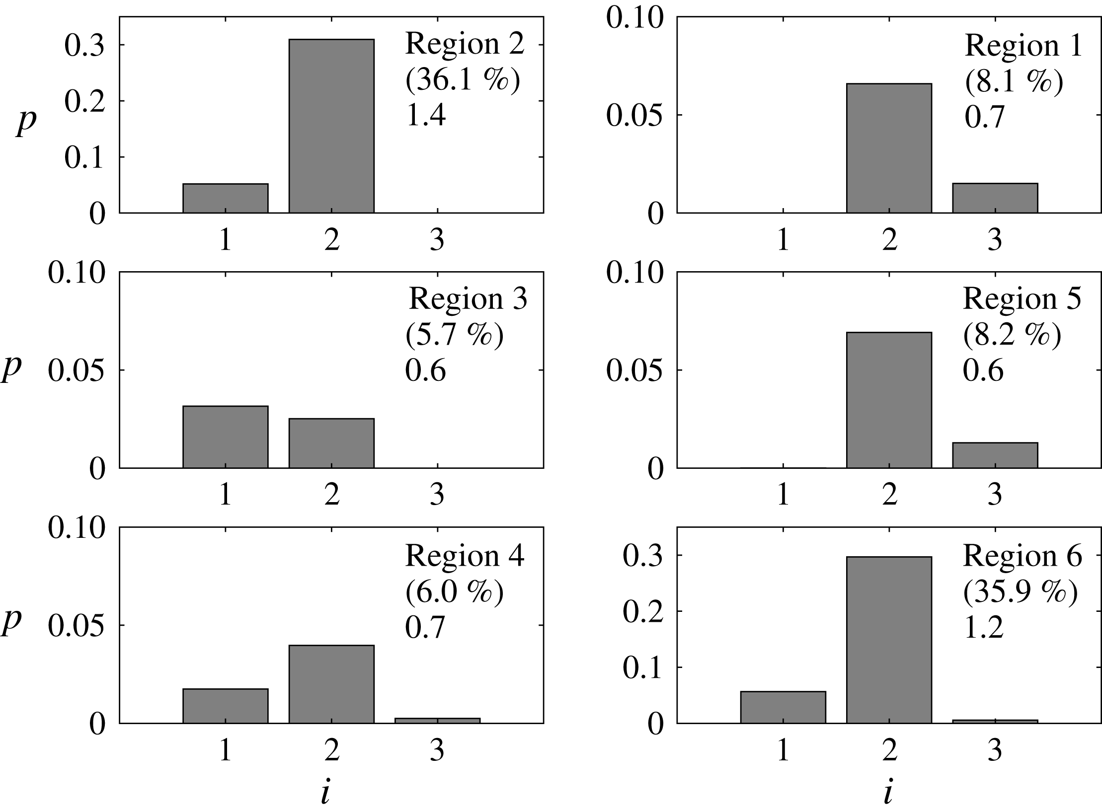
Given
 $\unicode[STIX]{x1D703}_{i}^{A,A}>0.985$
, the bars show the probability of the alignments for particular
 $i$
. The percentage value in brackets in each panel is the sum of the values in each panel. The number beneath this is the ratio between this percentage and that given for this region of the
 $\unicode[STIX]{x1D64C}_{A}{-}\unicode[STIX]{x1D64D}_{A}$
diagram in table 1.

The vorticity vector,
 $\unicode[STIX]{x1D74E}^{A}$
, is typically most strongly aligned with
 $\boldsymbol{e}_{2}^{A}$
than
 $\boldsymbol{e}_{1}^{A}$
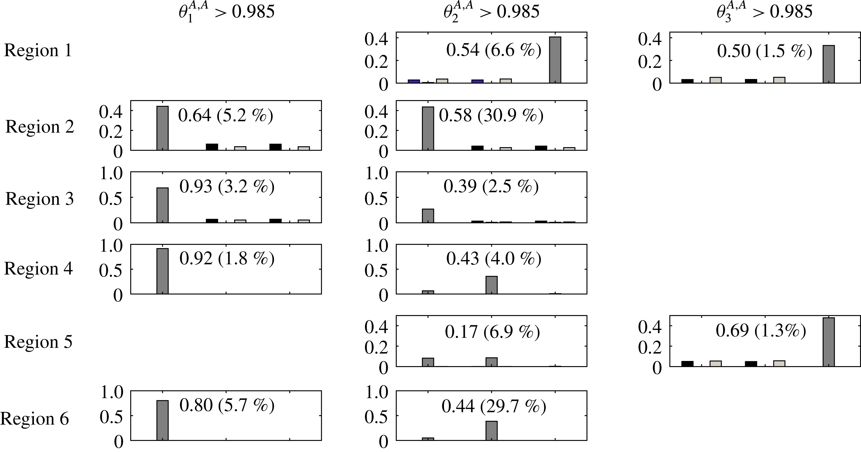
(Kerr Reference Kerr1985; Tsinober Reference Tsinober, Hunt and Vassilicos2001). The probability distributions for these alignments are shown in figure 13. Extracting the cases where a strong alignment exists, i.e.
 $\unicode[STIX]{x1D703}_{i}^{A,A}>0.985$
(
 $\pm 10^{\circ }$
), the results can be synthesized into the bar graphs shown in figure 14. This highlights the high proportion of
 $\unicode[STIX]{x1D703}_{i}^{A,A}>0.985$
occurrences in regions 2 and 6 (
 ${\sim}36\,\%$
of the total in both cases). These are also the two regions that HIT occupies preferentially relative to random, synthetic tensors with appropriate bounds on their non-normality (Keylock Reference Keylock2017). These relative proportions for strong alignment cases are 1.4 times and 1.2 times higher than the general occupancy proportions for these regions. Overall, 81 % of cases where
 $\unicode[STIX]{x1D703}_{i}^{A,A}>0.985$
occur for
 $\unicode[STIX]{x1D703}_{2}^{A,A}$
, with 16 % for
 $\unicode[STIX]{x1D703}_{1}^{A,A}$
. The propensity for alignment with
 $\unicode[STIX]{x1D703}_{1}^{A,A}$
and
 $\unicode[STIX]{x1D703}_{3}^{A,A}$
is dictated by the sign of
 $\unicode[STIX]{x1D64D}_{A}$
where
 $\unicode[STIX]{x1D6E5}_{L}>0$
and is dominated by
 $\unicode[STIX]{x1D703}_{1}^{A,A}$
below the discriminant function. Region 3 is the only part of the
 $\unicode[STIX]{x1D64C}_{A}{-}\unicode[STIX]{x1D64D}_{A}$
diagram where
 $\unicode[STIX]{x1D703}_{2}^{A,A}$
alignments are of secondary likelihood.
The probability of attaining different values for
 $\unicode[STIX]{x1D709}$
as a function of the four regions of the
 $\unicode[STIX]{x1D64C}_{A}{-}\unicode[STIX]{x1D64D}_{A}$
diagram where
 $\unicode[STIX]{x1D74E}^{B}$
is non-zero.

With the decomposition adopted in this study there are three vorticity vectors and nine strain eigenvectors, permitting analysis of mutual vorticity alignments (given by
 $\unicode[STIX]{x1D709}$
) or strain alignments (
 $\unicode[STIX]{x1D719}$
), as well as the vorticity–strain alignments (
 $\unicode[STIX]{x1D703}$
). In the sub-sections below, the primary findings in these respects are discussed.
6.2 Vorticity–vorticity alignments
In order to understand the
 $\unicode[STIX]{x1D703}_{i}^{A,A}$
alignments discussed above, the mutual vorticity vector alignments are discussed first. Note the important result that because there is no vorticity for
 $\unicode[STIX]{x1D63D}$
beneath the discriminant function then there has to be perfect alignment between the
 $\unicode[STIX]{x1D63C}$
and
 $\unicode[STIX]{x1D63E}$
vorticity vectors and
 $\unicode[STIX]{x1D709}^{A,C}=1$
. Thus, focus is on the four regions where
 $\unicode[STIX]{x1D6E5}_{L}>0$
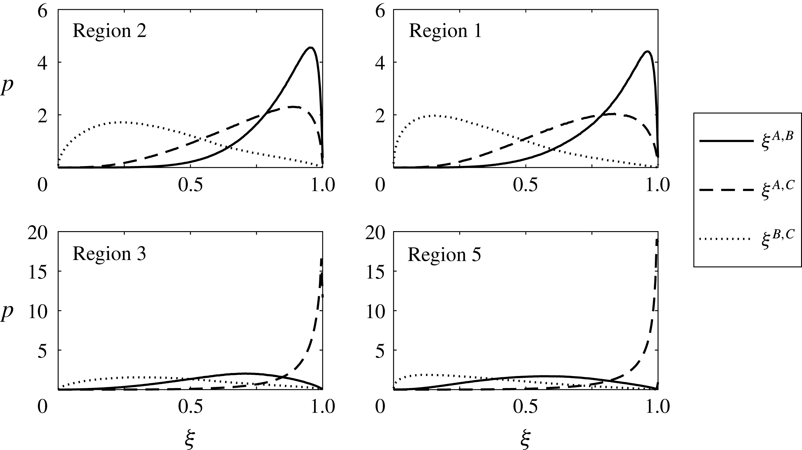
in figure 15 and immediately above the discriminant function in regions 3 and 5, there is still a strong tendency for
 $\unicode[STIX]{x1D709}^{A,C}\rightarrow 1$
. However, when
 $\unicode[STIX]{x1D64C}_{A}>0$
this is a weaker effect, with a stronger alignment for
 $\unicode[STIX]{x1D709}^{A,B}$
emerging. The accompanying curves for
 $\unicode[STIX]{x1D709}^{B,C}$
show that there is very limited strong alignment between
 $\unicode[STIX]{x1D74E}^{B}$
and
 $\unicode[STIX]{x1D74E}^{C}$
, meaning there are two distinct sets of vorticity vectors in the positive
 $\unicode[STIX]{x1D64C}_{A}$
regions depending on these alignments. This provides the mechanism for the observation by Tsinober et al. (Reference Tsinober, Shtilman and Vaisburd1997) that points where the vorticity vector is aligned with the strain eigenvector for the maximal eigenvalue are a distinct set compared to those aligning with the intermediate eigenvector: the orientation of
 $\unicode[STIX]{x1D74E}^{A}$
is driven by either
 $\unicode[STIX]{x1D74E}^{B}$
or
 $\unicode[STIX]{x1D74E}^{C}$
in different locations.
6.3 Strain–strain eigenvector alignments
Given
 $\unicode[STIX]{x1D703}_{i}^{A,A}>0.985$
, results are shown for where any
 $\unicode[STIX]{x1D719}_{i,j}^{B,C}>0.985$
as a function of the strain eigenvector that dictates the
 $\unicode[STIX]{x1D703}_{i}^{A,A}>0.985$
state. Values for
 $i$
are given by each group of bars, while
 $j\in \{1,2,3\}$
are shown in black, grey and light grey, respectively. The number in each panel is the sum of the probabilities in each panel (which does not equate to 1 because not all
 $\unicode[STIX]{x1D719}_{i,j}^{B,C}$
values exceed 0.985). The percentage in each panel indicates the fraction of the total number of cases represented by the results in a specific panel. This sums to 99.3 %, with the remaining 0.7 % of cases occurring in the six panels that are not shown.

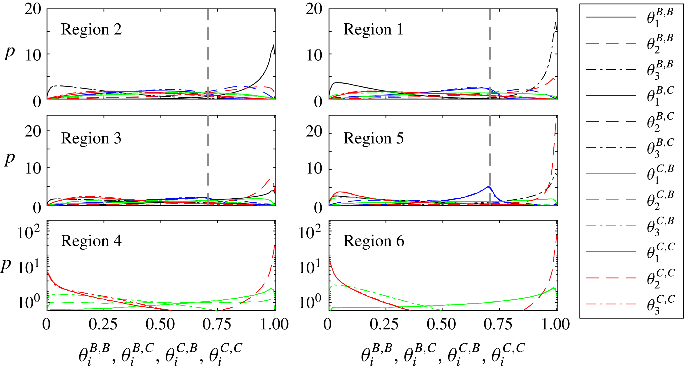
In figure 16, the strong strain–strain alignments,
 $\unicode[STIX]{x1D719}_{i,j}^{B,C}>0.985$
are shown, for the cases where strong alignments between the vorticity vector and strain eigenvectors for
 $\unicode[STIX]{x1D63C}$
have already been determined (i.e. the cases highlighted in figure 14). Each panel potentially contains nine bars representing the three values for
 $j$
(black, grey, white) as a function of the three values for
 $i$
given by the number on the
 $x$
-axis. From this diagram there is a sense of how mutual strain alignments are conditioning the observed behaviour for
 $\unicode[STIX]{x1D63C}$
.
The first thing to note is that not all of the eighteen possible panels are shown in this figure, as those excluded only represented 0.7 % of the total cases where
 $\unicode[STIX]{x1D719}_{i,j}^{B,C}>0.985$
(hence, the percentages in all twelve panels shown sum to 99.3 %). Secondly, when
 $\unicode[STIX]{x1D703}_{1}^{A,A}>0.985$
(the left-hand column of panels), strong strain–strain alignments are much more likely. Thus, when the vorticity vector for
 $\unicode[STIX]{x1D63C}$
is aligned with the eigenvector for the leading eigenvalue, there is a 64 %–93 % chance that there is a strong alignment for the strain eigenvectors for
 $\unicode[STIX]{x1D63D}$
and
 $\unicode[STIX]{x1D63E}$
. Almost exclusively, the strong alignment is for
 $\unicode[STIX]{x1D719}_{1,2}^{B,C}>0.985$
and these occurrences arise on the left-hand side of the
 $\unicode[STIX]{x1D64C}_{A}{-}\unicode[STIX]{x1D64D}_{A}$
diagram (regions 2, 3, 4) and beneath the discriminant function (regions 4 and 6). While
 $\unicode[STIX]{x1D703}_{3}^{A,A}>0.985$
only make up 2.8 % of cases (right-hand column), strong strain–strain alignments are also likely (50 %–69 % chance), are dominated by
 $\unicode[STIX]{x1D719}_{3,2}^{B,C}>0.985$
and occur on the right-hand side of the
 $\unicode[STIX]{x1D64C}_{A}{-}\unicode[STIX]{x1D64D}_{A}$
diagram above the discriminant function (regions 1 and 5). Hence, in both the left and right columns it is the intermediate eigenvector for
 $\unicode[STIX]{x1D63E}$
that dominates the strain–strain alignment.
Mutual strain–strain alignments are of reduced relative importance where
 $\unicode[STIX]{x1D703}_{2}^{A,A}>0.985$
(17 %–58 % likelihood). In regions 1, 2, and 3 the relation to the left and right sides of the
 $\unicode[STIX]{x1D64C}_{A}{-}\unicode[STIX]{x1D64D}_{A}$
diagram is preserved, with
 $\unicode[STIX]{x1D719}_{3,2}^{B,C}>0.985$
dominant in region 1 and
 $\unicode[STIX]{x1D719}_{1,2}^{B,C}>0.985$
in regions 2 and 3. However, in regions 4, 5 and 6, the most important strain–strain alignment where
 $\unicode[STIX]{x1D703}_{2}^{A,A}>0.985$
is between the two intermediate eigenvectors, i.e.
 $\unicode[STIX]{x1D719}_{2,2}^{B,C}>0.985$
.
In summary, strain–strain coupling between
 $\unicode[STIX]{x1D63D}$
and
 $\unicode[STIX]{x1D63E}$
is of greater importance for explaining vorticity–strain alignments for
 $\unicode[STIX]{x1D63C}$
when the alignment is not of the dominant, intermediate eigenvector type. However, irrespective of the nature of
 $\unicode[STIX]{x1D703}_{i}^{A,A}$
, alignments are with the intermediate eigenvector of
 $\unicode[STIX]{x1D63E}$
.
The distribution functions for the alignments,
 $\unicode[STIX]{x1D703}_{i}^{B,B}$
(black),
 $\unicode[STIX]{x1D703}_{i}^{B,C}$
(blue),
 $\unicode[STIX]{x1D703}_{i}^{C,B}$
(green) and
 $\unicode[STIX]{x1D703}_{i}^{C,C}$
(red) between the vorticity vector and the strain eigenvectors. The solid lines are for
 $i=1$
, the dashed lines are for
 $i=2$
and the dot-dashed lines are for
 $i=3$
. The vertical, dashed grey lines indicate an angle of
 $\pm 45^{\circ }$
.

6.4 Vorticity and strain alignments for
$\unicode[STIX]{x1D63D}$
and
$\unicode[STIX]{x1D63E}$


In addition to the mutual strain–strain and vorticity–vorticity alignments, it is also of interest to determine how the vorticity–strain alignments for
 $\unicode[STIX]{x1D63D}$
and
 $\unicode[STIX]{x1D63E}$
underpin the alignments for
 $\unicode[STIX]{x1D63C}$
. Figure 17 shows the probability curves for
 $\unicode[STIX]{x1D703}_{i}^{B,B}$
,
 $\unicode[STIX]{x1D703}_{i}^{B,C}$
,
 $\unicode[STIX]{x1D703}_{i}^{C,B}$
and
 $\unicode[STIX]{x1D703}_{i}^{C,C}$
. It is noticeable that strong alignments for particular terms are more probable where
 $\unicode[STIX]{x1D64D}_{A}>0$
in regions 1, 5 and 6. The absence of a rotation tensor for
 $\unicode[STIX]{x1D63D}$
beneath the discriminant function means that there are fewer alignments to evaluate in regions 4 and 6, and the results in this region are plotted using a logarithmic ordinate because strong
 $\unicode[STIX]{x1D703}_{2}^{C,C}$
alignments (red, dashed line) completely dominate the statistics. The importance of this alignment persists into regions 3 and 5, particularly in the latter case near the Vieillefosse tail. However, strong alignments for
 $\unicode[STIX]{x1D703}_{1}^{B,B}$
(solid, black line) and
 $\unicode[STIX]{x1D703}_{3}^{B,B}$
(dot-dashed, black line) emerge for regions 3 and 5, respectively, as
 $\unicode[STIX]{x1D74E}^{B}$
becomes non-zero, with these terms dominating the alignments in regions 1 and 2, where
 $\unicode[STIX]{x1D64C}_{A}>0$
. Given the strict structure to the eigenvalues for
 $\unicode[STIX]{x1D64E}_{B}$
, it is necessary that these alignments are coupled to the extensive (regions 2 and 3) and compressive (regions 1 and 5) eigenvalues for the rod-like and disc-like structures, respectively. The cross-terms (green and blue lines) are of more minor importance to the alignment structure. However, where they are defined,
 $\unicode[STIX]{x1D703}_{1}^{B,C}$
and
 $\unicode[STIX]{x1D703}_{3}^{B,C}$
have maxima at
 $\pm 45^{\circ }$
(highlighted by the vertical, grey, dashed line), and this effect is most pronounced in region 5. The terms that are most prone to exhibit orthogonality rather than alignment are
 $\unicode[STIX]{x1D703}_{3}^{C,B}$
(green, dot-dashed line) and
 $\unicode[STIX]{x1D703}_{1}^{C,C}$
(red, solid line). This effect is particularly true for the latter term and in regions 4 and 6. Overall, the region where one form of alignment does not really dominate is region 3, where both
 $\unicode[STIX]{x1D703}_{1}^{B,B}$
and
 $\unicode[STIX]{x1D703}_{2}^{C,C}$
are of similar likelihood. Thus, in this region, in particular, there are two mechanisms driving the alignments, which explains why large values for
 $\unicode[STIX]{x1D703}_{1}^{A,A}$
and
 $\unicode[STIX]{x1D703}_{2}^{A,A}$
are of similar probability in figure 13.
6.5 An explanation of observed alignments for
$\unicode[STIX]{x1D63C}$

Based on the above, previous observations on alignment structure may be reconsidered, focusing in particular on the intermediate
 $\unicode[STIX]{x1D703}_{2}^{A,A}$
alignment. Recalling from figure 15 that
 $\unicode[STIX]{x1D709}^{A,C}=1$
by definition in regions 4 and 6, then the dominance of the
 $\unicode[STIX]{x1D703}_{2}^{C,C}$
term in figure 17 demonstrates that the non-normal tensor drives vorticity–strain alignment beneath the discriminant function. A similar explanation still applies in region 5, where
 $\unicode[STIX]{x1D709}^{A,C}$
and
 $\unicode[STIX]{x1D703}_{2}^{C,C}$
are still dominant. However, the emergence of
 $\unicode[STIX]{x1D703}_{3}^{A,A}$
alignments is driven by
 $\unicode[STIX]{x1D703}_{3}^{B,B}$
in figure 17. Region 3 is similar to region 5 in that
 $\unicode[STIX]{x1D709}^{A,C}\rightarrow 1$
and there is a strong
 $\unicode[STIX]{x1D703}_{2}^{C,C}$
alignment in figure 17, explaining the intermediate eigenvector alignment for
 $\unicode[STIX]{x1D63C}$
. However, this is the region of the
 $\unicode[STIX]{x1D64C}_{A}{-}\unicode[STIX]{x1D64D}_{A}$
diagram where
 $\unicode[STIX]{x1D703}_{2}^{A,A}$
alignments are less probable than
 $\unicode[STIX]{x1D703}_{1}^{A,A}$
, and is also the region where strong
 $\unicode[STIX]{x1D719}_{i,j}^{B,C}$
alignments are the most probable given strong
 $\unicode[STIX]{x1D703}_{1}^{A,A}$
alignments, with the dominant term
 $\unicode[STIX]{x1D719}_{1,2}^{B,C}$
(figure 16). Hence, the strong mutual alignment of the strain eigenvectors means that
 $\unicode[STIX]{x1D703}_{1}^{A,A}$
can emerge where the normal straining is greater in magnitude, which is not infrequent (figure 3).
In regions 1 and 2, the normal mutual vorticity–strain alignments are dominant and occur with the third and first eigenvectors, respectively (figure 17). It is also the case that
 $\unicode[STIX]{x1D709}^{A,B}$
is more strongly aligned than
 $\unicode[STIX]{x1D709}^{A,C}$
, meaning that the emergence of
 $\unicode[STIX]{x1D703}_{2}^{A,A}$
as the dominant alignment is particularly surprising. In the context of the observation by Tsinober that this emerges because alignments with the primary eigenvector occurs on a different set of points, then figure 14 shows that alignments with the third eigenvector are not much less frequent when the different relative frequency of strong alignment occurrences between regions 1 (8.1 %) and 2 (36.1 %) is ignored. In either case, the kinematic properties readily explain the sub-dominant alignments with the first and third strain eigenvectors. That the intermediate eigenvector alignment dominates is then a consequence of the magnitude of the non-normal contributions to the dynamics. In particular, the strongly negative values for
 $\unicode[STIX]{x1D705}_{Q}^{(S)}$
in figure 3 show that straining is dominated by the non-normal terms. Furthermore, the top two panels in the central column of figure 16 show that when
 $\unicode[STIX]{x1D703}_{2}^{A,A}$
is the dominant alignment,
 $\unicode[STIX]{x1D719}_{3,2}^{B,C}>0.985$
or
 $\unicode[STIX]{x1D719}_{1,2}^{B,C}>0.985$
more frequently than elsewhere in the
 $\unicode[STIX]{x1D64C}_{A}{-}\unicode[STIX]{x1D64D}_{A}$
diagram. With the non-normal strain then greater in magnitude, the result is
 $\unicode[STIX]{x1D703}_{2}^{A,A}$
dominates
 $\unicode[STIX]{x1D703}_{1}^{A,A}$
, and
 $\unicode[STIX]{x1D703}_{3}^{A,A}$
. Hence, the intermediate alignment detected in the early direct numerical simulations of HIT (Kerr Reference Kerr1985; Ashurst et al.
Reference Ashurst, Kerstein, Kerr and Gibson1987) emerges as a direct consequence of the magnitude of non-normal effects in the vortical regions – the kinematics highlight stronger relations with
 $\unicode[STIX]{x1D63D}$
than
 $\unicode[STIX]{x1D63E}$
in regions 1 and 2, although elsewhere in the
 $\unicode[STIX]{x1D64C}_{A}{-}\unicode[STIX]{x1D64D}_{A}$
diagram, non-normal effects may dominate the kinematic relations.
7 Conclusion
A radical interpretation of the additive decomposition of the velocity gradient tensor,
 $\unicode[STIX]{x1D63C}$
into normal and non-normal tensors,
 $\unicode[STIX]{x1D63D}$
and
 $\unicode[STIX]{x1D63E}$
, is to state that while strain occurs everywhere, no net coherent enstrophy arises beneath the discriminant function of the
 $\unicode[STIX]{x1D64C}_{A}{-}\unicode[STIX]{x1D64D}_{A}$
diagram. Because the eigenvalues for
 $\unicode[STIX]{x1D64E}_{B}$
and
 $\unicode[STIX]{x1D734}_{B}$
are the real and imaginary parts of the eigenvalues for
 $\unicode[STIX]{x1D63C}$
, respectively, the latter does not exist in regions 4 and 6, and any observed vorticity comes from the non-normal contribution. However, because
 $\Vert \unicode[STIX]{x1D734}_{C}\Vert ^{2}=\Vert \unicode[STIX]{x1D64E}_{C}\Vert ^{2}$
, this is counter-balanced by a term contributing to the straining.
It was something of a surprise to fluid mechanics when the first direct numerical simulations of HIT showed a preferential alignment between the vorticity vector and the eigenvector for the second eigenvalue of the strain tensor rather than the first eigenvalue (Kerr Reference Kerr1985; Ashurst et al.
Reference Ashurst, Kerstein, Kerr and Gibson1987). This study has shown the critical role of non-normality in explaining this phenomenon. In regions 4 and 6 there is a perfect alignment between the vorticity vectors for
 $\unicode[STIX]{x1D63C}$
and
 $\unicode[STIX]{x1D63E}$
, i.e.
 $\unicode[STIX]{x1D709}^{A,C}=1$
, and this term still dominates in regions 3 and 5. Coupled to the tendency for the vorticity vector for
 $\unicode[STIX]{x1D63E}$
to align with the eigenvector for the intermediate strain eigenvalue for
 $\unicode[STIX]{x1D63E}$
, i.e.
 $\unicode[STIX]{x1D703}_{2}^{C,C}$
, this explains why
 $\unicode[STIX]{x1D703}_{2}^{A,A}$
is prevalent in these regions. In regions 1 and 2, where enstrophy dominates strain, the normal terms dominate the kinematic relations, which imply alignments with the first and third eigenvectors. However, the weak normal straining compared to the magnitude of the non-normal straining term ensures that dynamically, the
 $\unicode[STIX]{x1D703}_{2}^{A,A}$
term still emerges as dominant, given the strong strain–strain alignments between
 $\unicode[STIX]{x1D719}_{3,2}^{B,C}$
(region 1) and
 $\unicode[STIX]{x1D719}_{1,2}^{B,C}$
(region 2), as seen in figure 16.
In addition to the preference for
 $\unicode[STIX]{x1D703}_{2}^{A,A}$
to be the dominant alignment in HIT, we have also investigated the well-known property for the strain eigenvalues for turbulence to tend towards disc-like rather than rod-like structures. Simply considering the strain eigenvalues, then it should be regions 1, 5 and 6 on the right-hand side of the
 $\unicode[STIX]{x1D64C}_{A}{-}\unicode[STIX]{x1D64D}_{A}$
diagram that drive the tendency for the formation of disc-like structures, and homogeneous, isotropic turbulence is in these three regions on about 55 % of occasions. However, the teardrop shape of the
 $\unicode[STIX]{x1D64C}_{A}{-}\unicode[STIX]{x1D64D}_{A}$
diagram means that region 2 is occupied much more frequently than region 1 in the ratio 26.5 : 11.1. Non-normal straining effects are more important in the vortical regions, and there are two terms that arise: the non-normal production term occurs preferentially in region 1 and is approximately uniformly distributed, with no preference to drive the formation of rod- or disc-like structures. On the other hand, in region 2, the interaction term is dominant and this is strongly biased towards the creation of disc-like structures. As a consequence, even though the normal straining in region 2 is driving a tendency to form rod-like structures, this weak term is overridden by the magnitude of the interaction term. Thus, it is regions 2, 5 and 6 that drive the tendency to form disc-like structures, and these are expressed on 70 % of occurrences, leading to the dominance of disc-like over rod-like straining structure.
Our results highlight the difficulty of applying eigenvalue-focused thinking to the dynamics of complex systems such a turbulence. This is now well known in hydrodynamic stability where transient effects due to non-normality, characterized by the pseudospectra, explain the time scales for instabilities to emerge (Reddy, Schmid & Henningson Reference Reddy, Schmid and Henningson1993; Trefethen et al.
Reference Trefethen, Trefethen, Reddy and Driscoll1993; Trefethen & Embree Reference Trefethen and Embree2005). The results of this study, summarized above, show how important non-normal effects are for the dynamics, and this is particularly the case for the alignment of the vorticity vector with the intermediate strain eigenvector, as explained above. The advantage of the Schur transform in this respect is that the non-normality,
 $\unicode[STIX]{x1D649}$
is projected into the Schur matrix,
 $\unicode[STIX]{x1D64F}$
, where it can be treated in a similar way to the eigenvalues,
 $\unicode[STIX]{x1D6EC}$
. Hence, this permitted the definition of
 $\unicode[STIX]{x1D63D}=\unicode[STIX]{x1D650}\unicode[STIX]{x1D726}\unicode[STIX]{x1D650}^{\ast }$
and
 $\unicode[STIX]{x1D63E}=\unicode[STIX]{x1D650}\unicode[STIX]{x1D649}\unicode[STIX]{x1D650}^{\ast }$
in this paper. In contrast, the eigenvalue decomposition projects the non-normality into the departure of the eigenvectors from a unitary form, making it harder to directly compare normal (local) and non-normal (non-local) effects.
It is only really along the Vieillefosse tail that normal effects, in particular, normal straining, dominate the dynamics. This helps explain the success of the restricted Euler model (Cantwell Reference Cantwell1992) in approximating the dynamics of the VGT, but the more complex behaviour in regions 1, 2 and 3, in particular, demonstrates the difficulty of understanding the non-local effects that predominate without considering both the eigenvalues and the non-normal contributions. Regarding the latter, of particular importance is the non-normal contribution to the balance between enstrophy and strain,
 $\Vert \unicode[STIX]{x1D64E}_{C}\Vert$
, and the non-normal production and interaction production terms defined in table 2, all of which may be obtained from the equation for the evolution of strain and rotation in equation (2.14). The decomposition introduced here also permits metrics for turbulence behaviour to be reconsidered. The Lund and Rogers normalization of the strain eigenvalues may be expanded into constituent terms as shown in equation (2.24), while the existence of vorticity vectors and strain eigenvectors for
 $\unicode[STIX]{x1D63C}$
,
 $\unicode[STIX]{x1D63D}$
, and
 $\unicode[STIX]{x1D63E}$
permits alignment properties to be examined in a new way as defined in equations (2.25) to (2.27). These terms and metrics can serve as a basis for evaluating existing models for the dynamics of the VGT (Wilczek & Meneveau Reference Wilczek and Meneveau2014; Johnson & Meneveau Reference Johnson and Meneveau2016), and for formulating new models of this type.
Acknowledgements
This research was supported by a Royal Academy of Engineering/Leverhulme Trust Senior Research Fellowship LTSRF1516-12-89 awarded to the author. He is grateful to C. Meneveau at Johns Hopkins University, as well as J. C. Vassilicos and colleagues at the Department of Aeronautics, Imperial College London, for their hospitality while completing this research.
Appendix A. Proof of the existence of a Schur transform
A Schur transform (Schur Reference Schur1909) always exists for a
 $n\times n$
matrix,
 $\unicode[STIX]{x1D63C}$
 $$\begin{eqnarray}\displaystyle \unicode[STIX]{x1D63C}=\unicode[STIX]{x1D650}\unicode[STIX]{x1D64F}\unicode[STIX]{x1D650}^{\ast }, & & \displaystyle\end{eqnarray}$$
and this decomposition can be arrived at by induction on
 $n$
because the Schur transform implies a set of nested subspaces that are
 $\unicode[STIX]{x1D63C}$
invariant. Given that the columns of
 $\unicode[STIX]{x1D650}$
form an orthonormal basis, for
 $n=1$
,
 $\unicode[STIX]{x1D650}=1$
. For
 $n>1$
, if
 $\unicode[STIX]{x1D706}_{1}$
is an eigenvalue of
 $\unicode[STIX]{x1D63C}$
and then one may denote the set of all eigenvectors for
 $\unicode[STIX]{x1D706}$
as
 $\unicode[STIX]{x1D652}$
with orthogonal complement,
 $\unicode[STIX]{x1D652}^{\bot }$
. One may then choose arbitrary orthonormal bases
 $\unicode[STIX]{x1D654}_{1}$
and
 $\unicode[STIX]{x1D654}_{2}$
that span
 $\unicode[STIX]{x1D652}$
and
 $\unicode[STIX]{x1D652}^{\bot }$
, such that the following submatrices are obtained
 $$\begin{eqnarray}\left[\begin{array}{@{}cc@{}}\unicode[STIX]{x1D654}_{1} & \unicode[STIX]{x1D654}_{2}\end{array}\right]^{\ast }\unicode[STIX]{x1D63C}\left[\begin{array}{@{}cc@{}}\unicode[STIX]{x1D654}_{1} & \unicode[STIX]{x1D654}_{2}\end{array}\right]=\left[\begin{array}{@{}cc@{}}\unicode[STIX]{x1D706}_{1} & \unicode[STIX]{x1D63C}_{12}\\ 0 & \unicode[STIX]{x1D63C}_{22}\end{array}\right].\end{eqnarray}$$
The right-hand side yields the desired upper-triangular form for
 $\unicode[STIX]{x1D64F}$
apart from the submatrix
 $\unicode[STIX]{x1D63C}_{22}$
. Hence, using the hierarchical subspace concept and redefining the above subspaces with respect to
 $\unicode[STIX]{x1D63C}_{22}$
initially, and continuing with such operations
 $n-1$
times results in an upper triangular matrix that may be decomposed into a diagonal matrix of eigenvalues and the non-normality matrix,
 $\unicode[STIX]{x1D64F}=\unicode[STIX]{x1D647}+\unicode[STIX]{x1D649}$
, as desired.
The Schur transform (Schur Reference Schur1909) may be implemented in a complex or a real form, where the latter is only quasi-upper triangular if the eigenvalues are complex, with the conjugate pair forming a
 $2\times 2$
Jordan block. Hence, the complex form is adopted throughout this paper to avoid this eventuality.