1 Introduction
A common feature of isolated vortices is the time-dependent deformation or motion of their axes, a phenomenon referred to as ‘vortex wandering’ or ‘vortex meandering’ and commonly described as being long-wavelength and random. Vortex wandering has been observed in the laboratory (see Devenport et al. Reference Devenport, Rife, Liapis and Follin1996, for example) and behind flying aircraft and it is known that its amplitude is significantly increased in the presence of turbulent surroundings (Baker et al. Reference Baker, Barker, Bofah and Saffman1974; Beninati & Marshall Reference Beninati and Marshall2005; Bailey & Tavoularis Reference Bailey and Tavoularis2008; Beresh, Henfling & Spillers Reference Beresh, Henfling and Spillers2010; van Jaarsveld et al. Reference van Jaarsveld, Holten, Elsenaar, Trieling and van Heijst2011). Although it seems obvious that the properties of vortex wandering should depend on the properties of turbulent surroundings, the relationship between these two sets of properties has not yet been established. One of the challenges in ascertaining such a relationship is the presence of several potential modes of interactions. In addition to free-stream turbulence, external factors that are presumed to affect vortex wandering include wind tunnel boundary layer turbulence (Beresh et al. Reference Beresh, Henfling and Spillers2010; Igarashi et al. Reference Igarashi, Durbin, Hu, Waltermire and Wehrmeyer2011; Boudet et al. Reference Boudet, Cahuzac, Kausche and Jacob2015), vibrations of the vortex generator (Jacquin et al. Reference Jacquin, Fabre, Geffroy and Coustols2001) and other external disturbances. Examples of such interactions include distortions of the primary vortex by Biot–Savart induction produced by Kelvin–Helmholtz vortices that form in the shear layer of the vortex generating wing (Gursul & Xie Reference Gursul and Xie2000) and interactions between a primary vortex and additional vortices produced by the vortex generator, such as would occur in the multi-vortex wakes of complex lifting surfaces (Jacquin et al. Reference Jacquin, Fabre, Geffroy and Coustols2001). A recent direct numerical simulation of a Batchelor vortex demonstrated that boundary conditions impact the wandering of a vortex (Jammy, Hills & Birch Reference Jammy, Hills and Birch2014).
A different approach aimed at explaining the causes of vortex wandering has been to connect it with intrinsic properties of the vortex. In a recent investigation, vortex wandering has been associated with an azimuthal instability having a wavenumber mode of unity (Edstrand et al. Reference Edstrand, Davis, Schmid, Taira and Cattafesta2016). The same mode was found earlier to promote transient growth of perturbations (Antkowiak & Brancher Reference Antkowiak and Brancher2004) or bends in the form of long-wavelength Kelvin waves (Fabre & Jacquin Reference Fabre and Jacquin2004; Fabre, Sipp & Jacquin Reference Fabre, Sipp and Jacquin2006). The long-wavelength Kelvin waves, labelled D displacement waves by Fabre et al. (Reference Fabre, Sipp and Jacquin2006), displace sections of the vortex axis away from the undisturbed axis location, which generates self-induced motion through Biot–Savart induction (Rokhsaz, Foster & Miller Reference Rokhsaz, Foster and Miller2000). A number of studies of this transient growth mechanism have focused on the amplification of an optimal perturbation (Antkowiak & Brancher Reference Antkowiak and Brancher2004; Pradeep & Hussain Reference Pradeep and Hussain2006; Heaton & Peake Reference Heaton and Peake2007), but similar behaviour has also been observed under the action of stochastic forcing (Fontane, Brancher & Fabre Reference Fontane, Brancher and Fabre2008) or in the presence of turbulent surroundings (Hussain, Pradeep & Stout Reference Hussain, Pradeep and Stout2011). Stout & Hussain (Reference Stout and Hussain2016) have described an interaction mechanism by which azimuthally aligned vortices are produced in the proximity of the vortex via the re-alignment and stretching of the vorticity within the turbulence (Melander & Hussain Reference Melander and Hussain1993; Marshall & Beninati Reference Marshall and Beninati2005; Takahashi, Ishii & Miyazaki Reference Takahashi, Ishii and Miyazaki2005) and bending waves are introduced in the vortex by the azimuthally aligned structures.
When a vortex is immersed in strong turbulence, which has either been generated by independent means in the free stream or originates in the wake of the vortex generator, wandering has also been attributed to direct interactions between the vortex and the turbulent eddies through ‘bodily convection’ (Crow & Bate Reference Crow and Bate1976).
Investigations of vortex wandering characteristics have been traditionally hampered by the motion of the vortex itself, particularly when attempting to use probes to measure the local properties of the vortex (Baker et al. Reference Baker, Barker, Bofah and Saffman1974; Devenport et al. Reference Devenport, Rife, Liapis and Follin1996; Bailey, Tavoularis & Lee Reference Bailey, Tavoularis and Lee2006; Bailey & Tavoularis Reference Bailey and Tavoularis2008). Advances in particle image velocimetry (Heyes, Jones & Smith Reference Heyes, Jones and Smith2004; van Jaarsveld et al. Reference van Jaarsveld, Holten, Elsenaar, Trieling and van Heijst2011) and numerical simulation (Marshall & Beninati Reference Marshall and Beninati2005; Jammy et al. Reference Jammy, Hills and Birch2014) have made it possible to gain a holistic view of the vortex behaviour. Experimental evidence has demonstrated that the transverse position of the axis of a wandering vortex follows approximately a Gaussian probability distribution (Devenport et al. Reference Devenport, Rife, Liapis and Follin1996; Heyes et al. Reference Heyes, Jones and Smith2004; Bailey et al. Reference Bailey, Tavoularis and Lee2006; Bailey & Tavoularis Reference Bailey and Tavoularis2008; van Jaarsveld et al. Reference van Jaarsveld, Holten, Elsenaar, Trieling and van Heijst2011) and that the amplitude of motion increases with increasing streamwise distance (Mula et al. Reference Mula, Stephenson, Tinney and Sirohi2013) and decreasing vortex circulation. In contrast, Giuni & Green (Reference Giuni and Green2013) found that the wandering amplitude of a wing-tip vortex depended on the shape of the vortex generator: for a square-tipped wing, the wandering decreased with distance from the wing, whereas for a wing with a rounded tip, the wandering amplitude increased with distance. When, however, a vortex was immersed in turbulent surroundings, it has been universally observed that its wandering amplitude increased with increasing turbulent kinetic energy (Heyes et al. Reference Heyes, Jones and Smith2004; Bailey & Tavoularis Reference Bailey and Tavoularis2008; van Jaarsveld et al. Reference van Jaarsveld, Holten, Elsenaar, Trieling and van Heijst2011). In some cases, the normalisation of the wandering amplitude with the use of idealised internal vortex scales resulted in collapsing of results obtained under different conditions (Birch Reference Birch2012). In particular, van Jaarsveld et al. (Reference van Jaarsveld, Holten, Elsenaar, Trieling and van Heijst2011) suggested that vortex wandering is analogous to the dispersion of a passive scalar injected from a point source in homogeneous turbulence (Taylor Reference Taylor1921; Pope Reference Pope2000) and substituted the Lagrangian time scale of the turbulence by the turnover time of the vortex to describe the wandering amplitude in terms of the standard deviation of the turbulent fluctuations, the residence time of the vortex in the turbulence and the vortex core circulation.
Most experimental studies of vortex wandering characteristics have examined the amplitude of the motion but gave little attention to its wavelength or frequency distributions. Some experimental evidence (del Pino et al. Reference del Pino, López-Alonso, Parras and Fernandez-Feria2011), as well as stability analyses, indicate that the vortex wavelength is at least an order of magnitude larger than the core radius, but other authors suggested that the wandering motion has no dominant wavelength or frequency (Rokhsaz et al. Reference Rokhsaz, Foster and Miller2000; Beninati & Marshall Reference Beninati and Marshall2005).
To analyse the vortex wavelength distribution, one would need to have maps of the instantaneous vortex axis, whereas to get the wandering frequency content, one would need accurate time-resolved measurements of the velocity field of the wandering vortex, both of which are difficult to achieve experimentally. As a result, little information is available regarding the streamwise waveform of the vortex motion and its dependence on free-stream turbulence. This observation has provided motivation for the present work.
The objective of this study was to investigate the time-dependent motion of an isolated vortex immersed in strong free-stream turbulence, in which the size of the energy containing eddies was comparable to, or larger than, the size of the vortex core. We analysed the amplitude, wavelength and frequency of vortex motions and considered all possible mechanisms of direct interactions between the primary vortex and the turbulence. This work is a continuation of previous studies which reported time-averaged (Bailey et al. Reference Bailey, Tavoularis and Lee2006) and conditionally averaged (Bailey & Tavoularis Reference Bailey and Tavoularis2008) velocity measurements, as well as analysing these results to elucidate the effect of free-stream turbulence on properties of an isolated vortex. Like the previous studies, the present work considers a vortex immersed in statistically simple, nearly isotropic, grid-generated turbulence with different turbulence intensities and length scales. Besides further analysis of hot-wire signals in a wind tunnel flow, we have also analysed related measurements in a water tunnel, collected using laser-induced fluorescence and stereoscopic particle image velocimetry.
2 Experimental arrangements
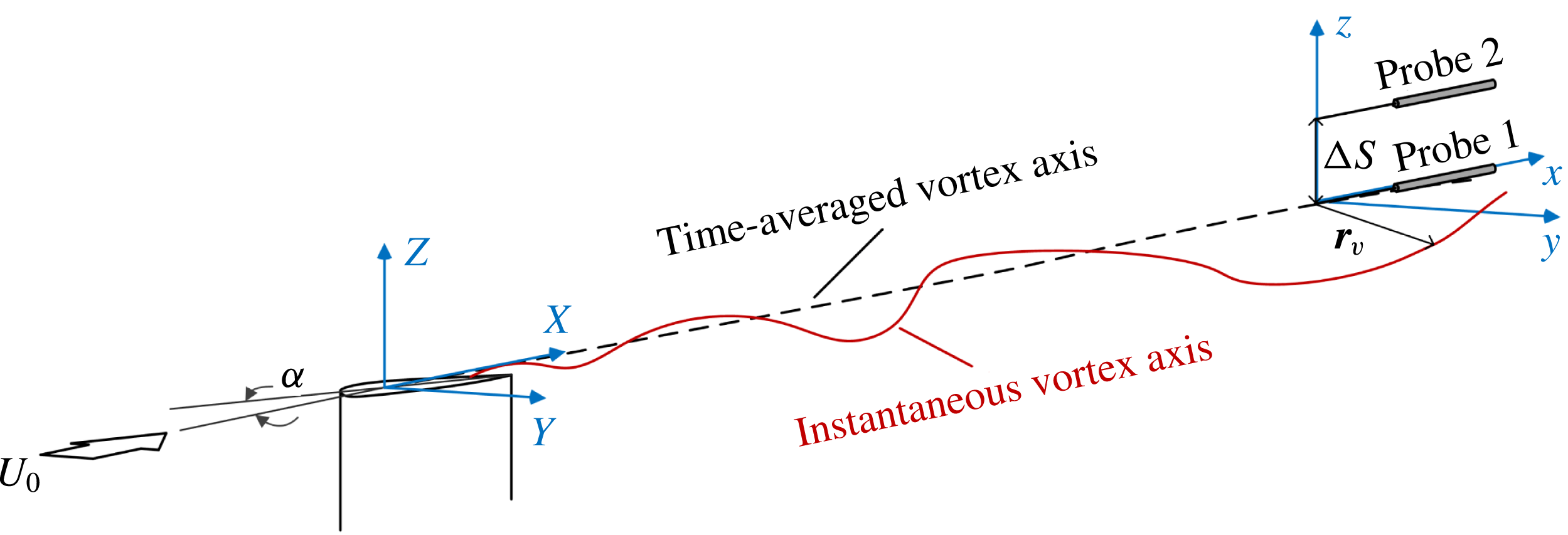
In all experiments, the vortex was generated at the tip of a wing and advected downstream, whereas free-stream turbulence was generated by a plate with square perforations (‘grid’) with a solidity of 0.44 upstream of the wing. The experimental configuration is sketched in figure 1, which also shows the definition of the two Cartesian coordinate systems used. The origin of the wing-fixed coordinate system
 $(X,Y,Z)$
is located at quarter chord on the wing-tip plane. The origin of the vortex-fixed coordinate system
 $(x,y,z)$
at a streamwise position
 $X$
is located at the corresponding time-averaged location of the vortex axis.
Schematic diagram of the experimental set-up, also showing the two coordinate systems used.

2.1 Wind tunnel tests
The present study utilises data from wind tunnel experiments previously reported by Bailey et al. (Reference Bailey, Tavoularis and Lee2006) and Bailey & Tavoularis (Reference Bailey and Tavoularis2008); additional details about the facility have been reported by Bailey (Reference Bailey2007). In these experiments the wing-tip vortex was generated in an open-circuit wind tunnel with a
 $0.60\times 0.90\times 3.66~\text{m}$
test section from a square-tipped NACA0012 wing at an angle of attack of
 $5^{\circ }$
. The wing had a chord length
 $c=178~\text{mm}$
, an aspect ratio of 2.9 and was equipped with a
 $0.58~\text{mm}$
diameter trip wire on the suction surface in order to induce bypass transition into the boundary layer and mitigate the possibility of leading-edge flow separation. Based on oil-film flow visualisation results, we concluded that the flow remained attached to the entire wing, despite its relatively short aspect ratio.
Nearly homogeneous and isotropic turbulence was generated by inserting a grid
 $4.29c$
upstream of the wing quarter-chord axis. Two grids were used with mesh sizes
 $M=50.8~\text{mm}$
(‘large grid’) and 25.4 mm (‘small grid’). With the wing removed, at the location of the wing axis the turbulence intensity and integral length scale were approximately 5 % and 25 mm for the large grid and 2.5 % and 15 mm for the small grid. In both cases, the turbulence decayed downstream in agreement with the literature (Bailey & Tavoularis Reference Bailey and Tavoularis2008).
For all tests, the free-stream velocity
 $U_{0}$
was approximately
 $20~\text{m}~\text{s}^{-1}$
so that the wing Reynolds number was
 $Re_{c}=U_{0}c/\unicode[STIX]{x1D708}\approx 2.4\times 10^{5}$
, where
 $\unicode[STIX]{x1D708}$
is the kinematic viscosity. The circulation
 $\unicode[STIX]{x1D6E4}$
was estimated by integrating radial profiles of the circumferential velocity at a radial distance of
 $0.4c$
from the time-averaged vortex axis (Bailey et al.
Reference Bailey, Tavoularis and Lee2006); the corresponding Reynolds number was
 $Re_{\unicode[STIX]{x1D6E4}}=\unicode[STIX]{x1D6E4}/\unicode[STIX]{x1D708}\approx 5\times 10^{4}$
.
Instantaneous two-point velocity measurements were acquired using two custom-built, four-sensor modified Kovasznay-type hot-wire probes, each with a measurement volume of approximately
 $0.5\times 0.5\times 0.5~\text{mm}^{3}$
. Signals from all eight sensors were sampled simultaneously at a rate of
 $f_{s}=30~\text{kHz}$
over 180 s and converted to velocity vectors using the approach of Wittmer, Devenport & Zsoldos (Reference Wittmer, Devenport and Zsoldos1998). Probe 1 was fixed at the time-averaged location of the vortex axis and probe 2 was separated from probe 1 in the
 $z$
-direction by a distance
 $\unicode[STIX]{x0394}S$
(figure 1). The instantaneous velocity vectors measured by the two probes are denoted as
 $\boldsymbol{U}_{1}$
and
 $\boldsymbol{U}_{2}$
, respectively.
Measurements were collected for each of the two grid cases as well as for a ‘no-grid’ case with the probes located at the streamwise positions
 $X/c=3.75$
, 5.75, 7.75 and 9.75. At each streamwise position, measurements were collected for 16 probe separations, adjusted with the use of a manually operated traversing system in increments of 0.5 mm in the range
 $7.1\leqslant \unicode[STIX]{x0394}S\leqslant 27.6~\text{mm}$
.
Bailey & Tavoularis (Reference Bailey and Tavoularis2008) have documented in detail single-point time-averaged properties of the vortex in a wandering frame of reference. Defining the radius
 $r^{\ast }$
of the vortex core as the location of the maximum circumferential velocity
 $U^{\ast }$
, they found that
 $U^{\ast }$
was in the range
 $0.2U_{0}\leqslant U^{\ast }\leqslant 0.4U_{0}$
, depending on the streamwise position and the free-stream turbulence characteristics, while in all cases
 $r^{\ast }\approx 8~\text{mm}$
. Note that within the coordinate system used, circumferential velocity is in the negative direction. For simplicity, within this paper we will omit the negative sign and refer to circumferential velocity and circulation by their magnitude.
2.2 Water tunnel tests
As complementary to the wind tunnel tests, additional experiments were conducted in a recirculating water tunnel with a free surface and a test section that was 0.55 m wide, 4 m long and filled with water to a depth of 0.70 m. The wing-tip vortex was also generated by a square-tipped NACA0012 rectangular wing with a chord length
 $c=178~\text{mm}$
at an angle of attack of
 $5^{\circ }$
; the aspect ratio of this wing was, however, 1.67. The wing was equipped with a 1 mm diameter trip wire on its suction surface and was mounted vertically with its root at the surface of the water such that its quarter-chord axis was in the centreplane of the tunnel test section and its tip was at a distance of
 $2.23c$
from the water tunnel floor. Free-surface ripple on the wing was avoided by mounting the root of the wing on a thin, bevelled, circular end plate with a diameter of
 $1.6c$
. The distances between the vortex and the bottom wall, the free surface and each of the side walls were, respectively and very approximately, 20, 15 and 13 core diameters, which were deemed to be sufficiently large for the vortex not to be strongly disturbed by boundary effects. The wing contained an internal reservoir, which was fed with water carrying dye and/or seeding particles through a tube connected to its root and was capable of injecting fluid into the flow through 0.4 mm diameter holes distributed near to and on the wing tip. Observation of dye injected from the wing surface and the tip demonstrated that, for the angle of attack of
 $5^{\circ }$
used in these tests, the flow did not separate from the wing surface.
Nearly homogeneous and isotropic turbulence was generated with the use of either of two perforated plates, also termed ‘large’ and ‘small’ grids with square perforations and positioned
 $3.8c$
upstream of the wing quarter-chord axis. The turbulence at the wing location with the wing removed had an intensity and a length scale that were approximately 6.8 % and 13 mm for the large grid (
 $M=50.8~\text{mm}$
) and 2.5 % and 11 mm for the small grid (
 $M=25.4~\text{mm}$
).
The unobstructed flow in the test section contained small periodic fluctuations, caused by shallow water waves, which are essentially unavoidable for flows in recirculating water tunnels with a free surface (Tavoularis Reference Tavoularis2005). These waves generated essentially bulk, rigid-body oscillations of the fluid in the water tunnel at a typical frequency of 0.1 Hz (Dunn Reference Dunn2004), which were superimposed on the grid turbulence. These oscillations maintained a fairly uniform amplitude along the test section, whereas grid turbulence decayed downstream and so, in an Eulerian frame of reference, the relative strength of the former increased with distance from the grid. In a Lagrangian frame of reference, however, surface waves did not affect the vortex wandering, as they travelled at the same speed. It was found that the turbulence kinetic energy per unit mass
 $k$
initially decayed with streamwise distance from the grid in a form described well by the conventional decay law (Comte-Bellot & Corrsin Reference Comte-Bellot and Corrsin1966), but, further downstream,
 $k$
seemed to tend towards constant asymptotes. In order to obtain a more meaningful measure of the local intensity of the free-stream motions that interacted with the vortex, we subtracted, in mean square, the unobstructed flow fluctuations from those measured with the grid in place. Considering that the shallow-wave-induced motions only affected the convection of the vortex as a whole and did not introduce local disturbances to it, we believe that the corrected turbulence intensity is more appropriate for comparisons with values in the wind tunnel. As expected, this correction was more appreciable for the small-grid than the large-grid results.
Turbulence and vortex properties were acquired primarily using a stereo particle image velocimetry (SPIV) system, which included a pulsed, dual Nd:YAG laser (New Wave Research, Model Solo 120XT) and two digital cameras (Imager pro X 4M) along with LaVision Inc., FlowMaster software for data processing. The laser was set to produce two pulses
 $3500~\unicode[STIX]{x03BC}\text{s}$
apart at a rate of
 $4~\text{Hz}$
. The cameras had a resolution of
 $2048\times 2048~\text{pixel}$
and were equipped with 50 mm lenses (Nikon Nikkor
 $f/1.8D$
) set at
 $f/2.8$
. In order to isolate laser light being reflected off the particles from ambient light and other reflections, 532.5 nm bandpass filters were used. The planes of measurement were parallel to the
 $YZ$
plane and vortex quantification measurements were taken at three planes downstream of the wing, namely, at
 $X/c=3.6$
, 6.6 and 12.8. The useful thickness of the laser sheet was approximately 2 mm. Hollow glass spheres (Potters Industries, Sphericel110P8), having a specific gravity of
 $1100~\text{kg}~\text{cm}^{-3}$
and a mean diameter of
 $11.7~\unicode[STIX]{x03BC}\text{m}$
, were used to seed the flow. The size of a particle was less than the size of a pixel in each image that was analysed and the average particle displacement between two images was eight pixels. The total uncertainty of each of the three measured velocity components was estimated to be in the range 3–4 %.
To examine the vortex wandering, laser-induced fluorescence (LIF) measurements were conducted using an aqueous solution of Rhodamine 6G fluorescent dye injected through the wing tip. Due to the rotation of the vortex, the dye remained in and near the vortex core along the test section. Illumination for all dye images was provided by a 1 W continuous beam diode laser (Wicked Lasers, model KPN5323S), with a peak wavelength of 532 nm. Two sets of images were recorded. As a means for reconstructing the instantaneous vortex axis shape, images were first acquired simultaneously at a rate of 4 Hz in two orthogonal planes containing the water tunnel axis, namely the
 $XY$
and
 $XZ$
planes; these images were taken using the same two cameras and lenses as those used for SPIV measurements and were centred at two positions,
 $X/c=6.6$
and 12.8. During these tests, the laser beam was passed through a lens to create a cone of light, which illuminated the entire vortex over the streamwise length that was in the field of view of the cameras. A second set of images was taken in the transverse, namely
 $YZ$
, plane. For these, the beam was passed through a lens that generated a sheet of light with a thickness of approximately 2 mm. Images in the transverse plane were taken with a high-speed camera (PCO pco.edge), equipped with a 50 mm
 $f/1.8\text{D}$
lens and a long pass 540 nm filter, which was mounted beside the water tunnel in the same arrangement as was used for the SPIV measurements. This camera was set at a resolution of
 $2560~\text{pixel}\times 2160~\text{pixel}$
and a frame rate of 100 Hz. Images in the
 $YZ$
plane were recorded only at
 $X/c=9.7$
.
Of concern in our study was whether the wandering vortex axis inclination with respect to the streamwise direction introduced significant errors in our SPIV measurements. Based on LIF image analysis, and after the addition of a maximum error of
 $2^{\circ }$
for undetectable misalignment of the camera with the intended viewing plane, we estimated the mean axis inclination angle to be
 $6^{\circ }{-}7^{\circ }$
for the no-grid case,
 $7^{\circ }{-}10^{\circ }$
for the small-grid case and
 $14^{\circ }$
for the large-grid case at
 $X/c=6.6$
. The corresponding uncertainties in the determination of the circumferential and axial velocity components were 0.5–0.7 %, 0.7–1.5 % and 3.0 %.
For all cases, the free-stream velocity
 $U_{0}$
was approximately
 $0.136~\text{m}~\text{s}^{-1}$
resulting in a chord Reynolds number
 $Re_{c}\approx 2.4\times 10^{4}$
, which is an order of magnitude smaller than that in the wind tunnel tests. Data from the SPIV experiments indicated that the vortex core had a radius
 $r^{\ast }$
that increased with downstream distance from 8 to 13 mm and a maximum circumferential velocity that was in the range
 $0.1U_{0}\leqslant U^{\ast }\leqslant 0.2U_{0}$
, depending on the streamwise position of the vortex and the free-stream turbulence characteristics. The Reynolds number based on vortex circulation is estimated to have been
 $Re_{\unicode[STIX]{x1D6E4}}\approx 3\times 10^{3}$
. Further details of the experimental results, including measured vortex properties and an extensive uncertainty analysis, have been reported by Pentelow (Reference Pentelow2014).
3 Procedures for the determination of the instantaneous vortex position
3.1 Determination of the instantaneous vortex axis location from two-point measurements
Time series of the vortex axis position under different conditions were reconstructed with the use of the following analysis, which couples the time series of velocities measured in the wind tunnel by the two probes with time-averaged properties of the vortex. To keep the computational time of the analysis relatively short, only the first 60 s of signals with probe separation in the range
 $7.1\leqslant \unicode[STIX]{x0394}S\leqslant 18.1~\text{mm}$
were considered. Comparison with analysis conducted on shorter segments of the time series indicated that statistical convergence of the results presented here was achieved prior to 60 s.
Let
 $\{\boldsymbol{e}_{y},\boldsymbol{e}_{z}\}$
be a two-dimensional Cartesian basis with its origin on the time-averaged vortex axis at location
 $X$
, such that a point in the measurement plane is specified by
 $\boldsymbol{r}=y\boldsymbol{e}_{y}+z\boldsymbol{e}_{z}$
. The positions of the two probes in this plane would therefore be
 $\boldsymbol{r}_{1}=0\boldsymbol{e}_{y}+0\boldsymbol{e}_{z}$
and
 $\boldsymbol{r}_{2}=0\boldsymbol{e}_{y}+\unicode[STIX]{x0394}S\boldsymbol{e}_{z}$
. We will denote the velocity vectors measured by probe 1 and probe 2 at time
 $t$
by
 $\boldsymbol{U}_{1}(t,\boldsymbol{r}_{1})=U_{y_{1}}\boldsymbol{e}_{y}+U_{z_{1}}\boldsymbol{e}_{z}$
and
 $\boldsymbol{U}_{2}(t,\boldsymbol{r}_{2})=U_{y_{2}}\boldsymbol{e}_{y}+U_{z_{2}}\boldsymbol{e}_{z}$
, respectively. To proceed, we will assume that an instantaneous velocity field
 $\boldsymbol{U}_{I}(\boldsymbol{r})$
was produced at a specific
 $X$
location and for specific free-stream turbulence conditions by an axisymmetric vortex centred at a location
 $\boldsymbol{r}_{g}=y_{g}\boldsymbol{e}_{y}+z_{g}\boldsymbol{e}_{z}$
and having a velocity profile approximated by the corresponding time-averaged velocity field, as estimated by Bailey & Tavoularis (Reference Bailey and Tavoularis2008).
A cost function was then defined as
 $$\begin{eqnarray}\unicode[STIX]{x1D700}(t,\boldsymbol{r}_{g})=\Vert \boldsymbol{U}_{1}(t,\boldsymbol{r}_{1})-\boldsymbol{U}_{I}(\boldsymbol{r}_{1})\Vert +\Vert \boldsymbol{U}_{2}(t,\boldsymbol{r}_{2})-\boldsymbol{U}_{I}(\boldsymbol{r}_{2})\Vert ,\end{eqnarray}$$
where
 $\Vert \cdot \Vert$
indicates the
 $L_{2}$
norm. This cost function was evaluated within the range
 $|y_{g}|\leqslant 30~\text{mm}$
and
 $|z_{g}|\leqslant 30~\text{mm}$
at discrete locations with spacings
 $\unicode[STIX]{x0394}y_{g}=0.006~\text{mm}$
and
 $\unicode[STIX]{x0394}z_{g}=0.006~\text{mm}$
. The most probable location
 $\boldsymbol{r}_{v}$
of the vortex axis at time
 $t$
was then determined as the location
 $\boldsymbol{r}_{g}$
at which the value of
 $\unicode[STIX]{x1D700}(t,\boldsymbol{r}_{g})$
was minimum. The entire process was then repeated for time increments equal to
 $1/f_{s}$
, resulting in a time series of the vortex axis position
 $\boldsymbol{r}_{v}(t)=y_{v}(t)\boldsymbol{e}_{y}+z_{v}(t)\boldsymbol{e}_{z}$
.
After a first data processing pass, occasional events could be observed in the vortex trajectory which appeared as large excursions in vortex position, following which the vortex almost immediately returned to a position close to the previous one. These instances were identified as probable mis-identification events. To quantify and remove these events, an automated outlier detection scheme was employed, which located instances at which the magnitude of the vortex acceleration deviated from the mean (which was approximately zero) by more than three standard deviations. The position values at these instances were discarded and replaced by values estimated by interpolation; such outliers accounted for less than 0.1 % of the entire time series. The analysis was repeated for
 $\unicode[STIX]{x0394}S$
from 7.1 to 18.1 mm with 0.5 mm increments, resulting in an ensemble of 22 time series of vortex axis position for each
 $X$
measurement location and set of free-stream turbulence conditions.
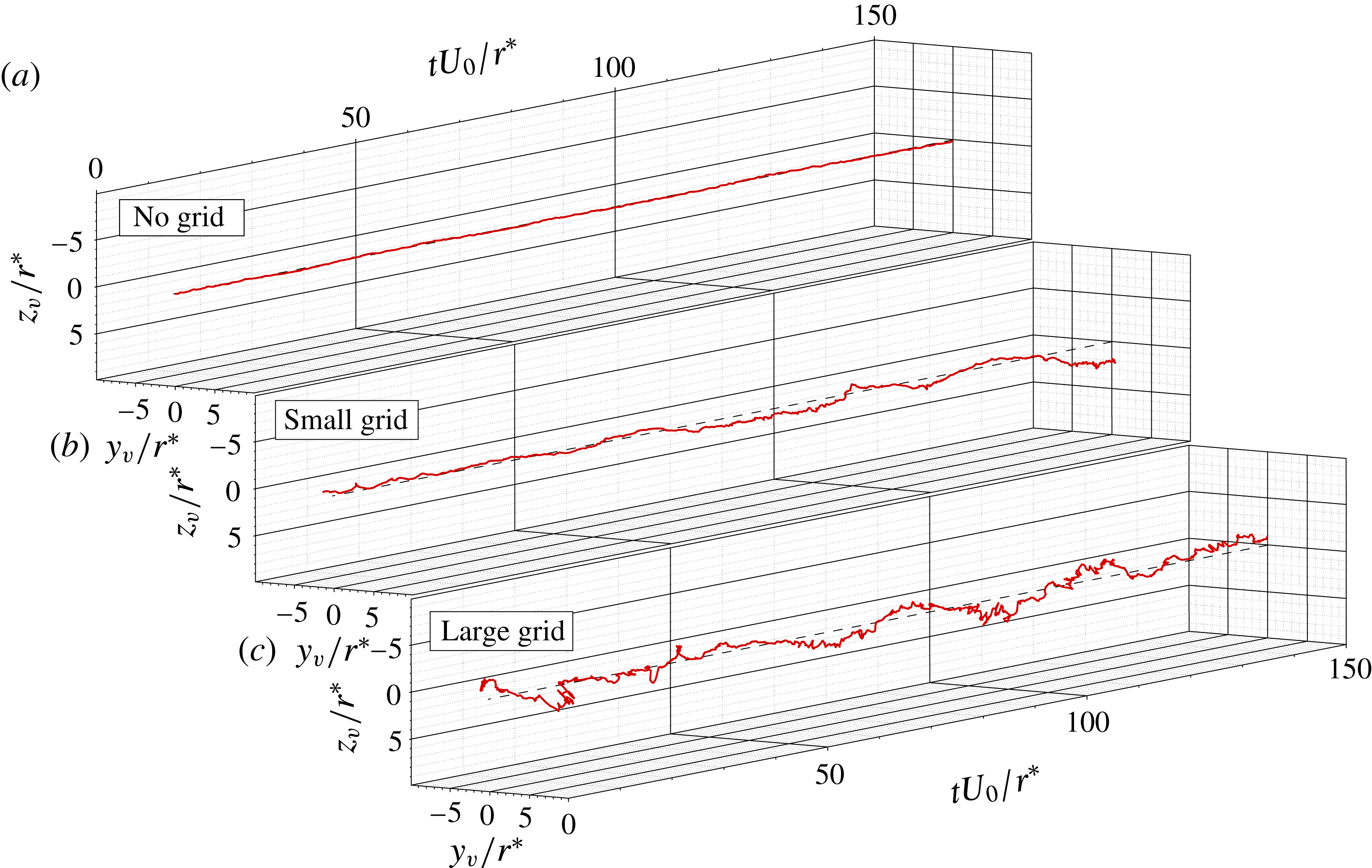
Sample segments of extracted time series of vortex axis position for (a) no-grid, (b) small-grid and (c) large-grid cases at
 $X/c=9.75$
. Dashed lines mark the corresponding time-averaged vortex positions.

Figure 2 shows representative segments of the time series of vortex axis position
 $\boldsymbol{r}_{v}(t)$
estimated at
 $X/c=9.75$
for the no-grid, small-grid and large-grid cases. In all three cases, the vortex axis was found to follow an apparently stochastic motion about the time-averaged vortex axis, and the magnitude of the deviations increased with increasing free-stream turbulence intensity. The large-grid case, in particular, also shows strong localised distortions in vortex trajectory, characterised by sharp bending of the vortex axis.
For a rough evaluation of the sensitivity of the present vortex trajectory reconstruction to the assumed form of
 $\boldsymbol{U}_{I}(\boldsymbol{r})$
, we tested this procedure using the synthetic velocity field of a Lamb–Oseen vortex. This vortex had prescribed radius
 $\tilde{r}$
and maximum circumferential velocity
 $\tilde{U}$
and its axis wandered on a cross-plane in a way that its coordinates were given by
 ${\tilde{y}}=A_{y}\sin (2\unicode[STIX]{x03C0}f_{y}t)$
and
 $\tilde{z}=A_{z}\sin (2\unicode[STIX]{x03C0}f_{z}t)$
, where
 $A_{y}$
and
 $A_{z}$
were prescribed wandering amplitudes and
 $f_{z}$
and
 $f_{y}$
were prescribed wandering frequencies, which are equivalent to the wavelengths
 $U_{0}\,f_{y}$
and
 $U_{0}\,f_{z}$
. The velocity time traces at
 $\boldsymbol{r}_{1}$
and
 $\boldsymbol{r}_{2}$
in this synthetic velocity field were extracted and analysed following the previously described procedure, in which the velocity profile
 $\boldsymbol{U}_{I}(\boldsymbol{r})$
was assumed to be equal to the time-averaged velocity profile estimated by Bailey & Tavoularis (Reference Bailey and Tavoularis2008) for the small-grid case at
 $X=5.75c$
. The analysis was repeated for several combinations of values of
 $\tilde{r}$
,
 $\tilde{U}$
,
 $A_{y}$
,
 $A_{z}$
,
 $f_{z}$
and
 $f_{y}$
within appropriate ranges. The analysis confirmed that, when the parameters (namely, the core radius and the maximum circumferential velocity) of the Lamb–Oseen vortex coincided with those of
 $\boldsymbol{U}_{I}(\boldsymbol{r})$
, the reconstructed axis traces reproduced closely the time series of
 ${\tilde{y}}$
and
 $\tilde{z}$
. As, however, the differences between the parameters of the Lamb–Oseen vortex and those of
 $\boldsymbol{U}_{I}(\boldsymbol{r})$
were increased, there were proportional increases in the differences between the reconstructed and prescribed values of the wandering amplitudes
 $A_{y}$
and
 $A_{z}$
. Even so, the reconstructed values of
 $f_{y}$
and
 $f_{z}$
were found to be quite insensitive to differences between the corresponding parameters of the two vortices, which demonstrates that small inaccuracies in the prescribed velocity profiles would have little effect on the reconstructed wandering wavelengths.
A formal uncertainty propagation analysis for the determination of the wandering amplitude by the previous method was not feasible, because the instantaneous velocity field of the vortex was time-dependent and we had no way of quantifying the differences between instantaneous and mean profiles. Although we were unable to estimate the bias limit of the wandering amplitude, we estimated that its precision uncertainty was less than 1.5 mm (
 $0.2r^{\ast }$
); this was achieved by comparing values computed by applying the analysis to measurements of probes with different separations. Moreover, estimates of wandering velocities and spectra of wandering motions computed from measurements of probes with different separations differed by less than 10 % of each other. In view of these results, we are confident that our methodology was sufficiently accurate to support our conclusions.
3.2 Reconstruction of the instantaneous vortex axis from LIF images
Sections of the vortex axis were reconstructed in three dimensions from images of fluorescent dye taken simultaneously in the
 $XY$
and
 $XZ$
planes. After testing several automated methods for identifying the vortex axis in each image, it was concluded that the most reliable method was visual inspection, which allowed us to distinguish clearly dye in the core of the vortex from dye present in peripheral structures. The rotation of the vortex facilitated this identification. The uncertainty in vortex axis location by this method was estimated to be
 $0.5r^{\ast }$
. Representative images with traced axes for the no-grid, small-grid and large-grid cases are shown in figure 3. The instantaneous spanwise
 $y_{v}$
and transverse
 $z_{v}$
components of the vortex axis position were then specified as functions of streamwise location. This technique was successful for all images except those taken near
 $X/c=12.8$
in the large-grid case. In that case, the vortex axis was not distinct enough to be confidently identified by this technique and so results from these images have not been included in subsequent analyses.
Two-hundred pairs of images in the
 $XY$
and
 $XZ$
planes were recorded for each free-stream condition. Each image was de-warped and scaled to actual dimensions with the use of a calibration plate with known dimensions using the manufacturer’s software (FlowMaster software, LaVision Inc.). The usable part of each scaled image, which excluded regions near the edges of the frame where lighting was insufficient for core identification, had a streamwise length of
 $0.75c$
and was centred at approximately
 $X/c=6.6$
or 12.8. The vortex axis was traced manually in each of the 200 frames in each of the
 $XY$
and
 $XZ$
planes and the assigned coordinates were fitted by a ninth-order polynomial of streamwise location
 $X$
; this fitted polynomial order was chosen among other values tried, as it seemed to capture the vortex axis shape without reproducing small-scale distortions that could be the result of the limited resolution of the coordinate recognition process. Finally, a continuous linear representation of the vortex axis in three dimensions was constructed by evaluating these polynomials over the streamwise extent of each pair of images.
Representative LIF images in the
 $XZ$
plane for the (a) no-grid, (b) small-grid and (c) large-grid cases at
 $X/c=6.6$
. Black lines mark the vortex axis and surrounding highlighted regions mark uncertainty bounds in vortex axis location; arrows indicate locations of secondary azimuthal structures; this annotation was added manually to each image during post-processing. Although the location of the axis may not be clearly visible in some still images, vortex rotation between subsequent images in a video sequence made it quite apparent.

The coordinates of the vortex axis on each dye image were determined by evaluating the corresponding fitted polynomials in the
 $XY$
and
 $XZ$
planes at
 $X/c=6.6$
and 12.8, which coincide with SPIV measurement planes, thus allowing comparisons. At these locations, the illumination of the dye was strong and the vortex core could be identified with high confidence. The standard deviations of the resulting series of vortex axis coordinates
 $\unicode[STIX]{x1D70E}_{y}$
and
 $\unicode[STIX]{x1D70E}_{z}$
for each set of images have been reported by Pentelow (Reference Pentelow2014).
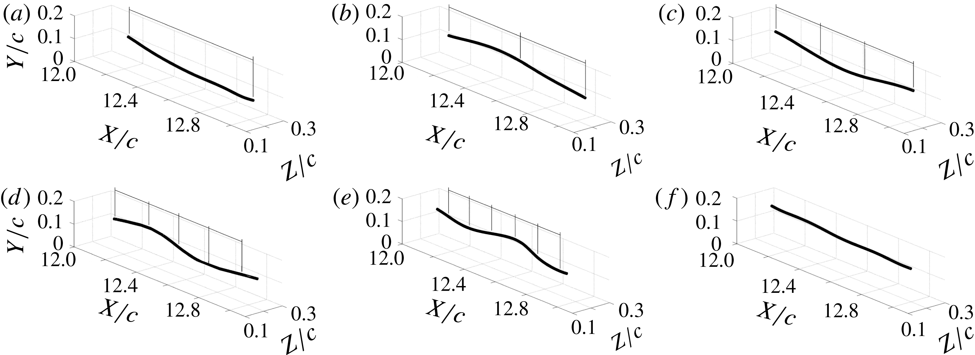
To discern any possible patterns in vortex axis shape in the water tunnel study, three-dimensional animated sequences of the reconstructed vortex axis were observed repeatedly from different points of view. It was noticed that the instantaneous vortex axis waveform was often nearly planar, and lay on a plane that included the streamwise axis but varied in orientation from one frame to the next. In this plane, the vortex axis often appeared to have a quasi-sinusoidal shape with a wavelength
 $\unicode[STIX]{x1D706}$
, whose value was estimated from the view in which such a quasi-sinusoidal waveform, if it existed at all, appeared to be most prominent. Representative examples are shown in figure 4; it is noted, however, that in many frames it was not possible to detect the presence of such waves.
The instantaneous axis position at
 $X/c=9.7$
was also determined from the LIF images on the
 $YZ$
plane. Following comparison of several methods for determining this axis, it was concluded that the centre of rotation of the dye patterns was a more accurate representation of the location of the vortex axis than the centroid of these patterns. The location of the centre of rotation was identified visually for each image by examining three sequential images in rapid succession and recording where the location of the apparent centre of rotation was for the final frame. This method was used for images from the no- and small-grid cases, although it was rarely possible to identify a centre about which the dye patterns were rotating in the dye images from the large-grid cases. Thus, vortex axis locations were not obtained from those images. Statistical analysis provided the average location of the vortex axis and the standard deviations of wandering distances along the
 $Y$
and
 $Z$
directions.
Examples of reconstructed vortex axes, in which the visible length appears to be (a) a quarter of a wavelength, (b) half a wavelength, (c) three-quarters of a wavelength, (d) a full wavelength, (e) one and a quarter wavelength or (f) not distinguishable as part of a wave.

4 Results
4.1 Wandering amplitudes
Our wind and water tunnel experiments have provided several independent estimates of the standard deviations
 $\unicode[STIX]{x1D70E}_{y}$
and
 $\unicode[STIX]{x1D70E}_{z}$
(‘wandering amplitudes’) of the vortex axis coordinates in the
 $y$
and
 $z$
directions. Such wandering amplitudes for the wind tunnel tests were determined from the time series of the components of the vortex axis position vector
 $\boldsymbol{r}_{v}(t)$
(§ 3.1) and averaged over ensembles of measurements obtained with different probe separations
 $\unicode[STIX]{x0394}S$
at the same
 $X$
. These estimates were compared to independent estimates of the same properties obtained with the use of a single-probe signal analysis by Bailey & Tavoularis (Reference Bailey and Tavoularis2008), under the assumption that the vortex axis crossed the probe location when the measured velocity components in the
 $yz$
plane vanished simultaneously. That study obtained the joint probability density function of vortex position by traversing the measurement probe throughout the
 $yz$
plane and counting the instances at which the in-plane velocity was zero; its results were within 15 % of estimates obtained using the approach of Devenport et al. (Reference Devenport, Rife, Liapis and Follin1996). Vortex wandering amplitudes for the water tunnel results were estimated by three different methods: (i) from the SPIV measurements on transverse planes; (ii) from the polynomials fitted to the reconstructed vortex axis that was identified in the simultaneous pairs of LIF images on streamwise planes; and (iii) from the LIF images on transverse planes. The wandering amplitudes estimated with the use of these techniques were within 25 % of each other.
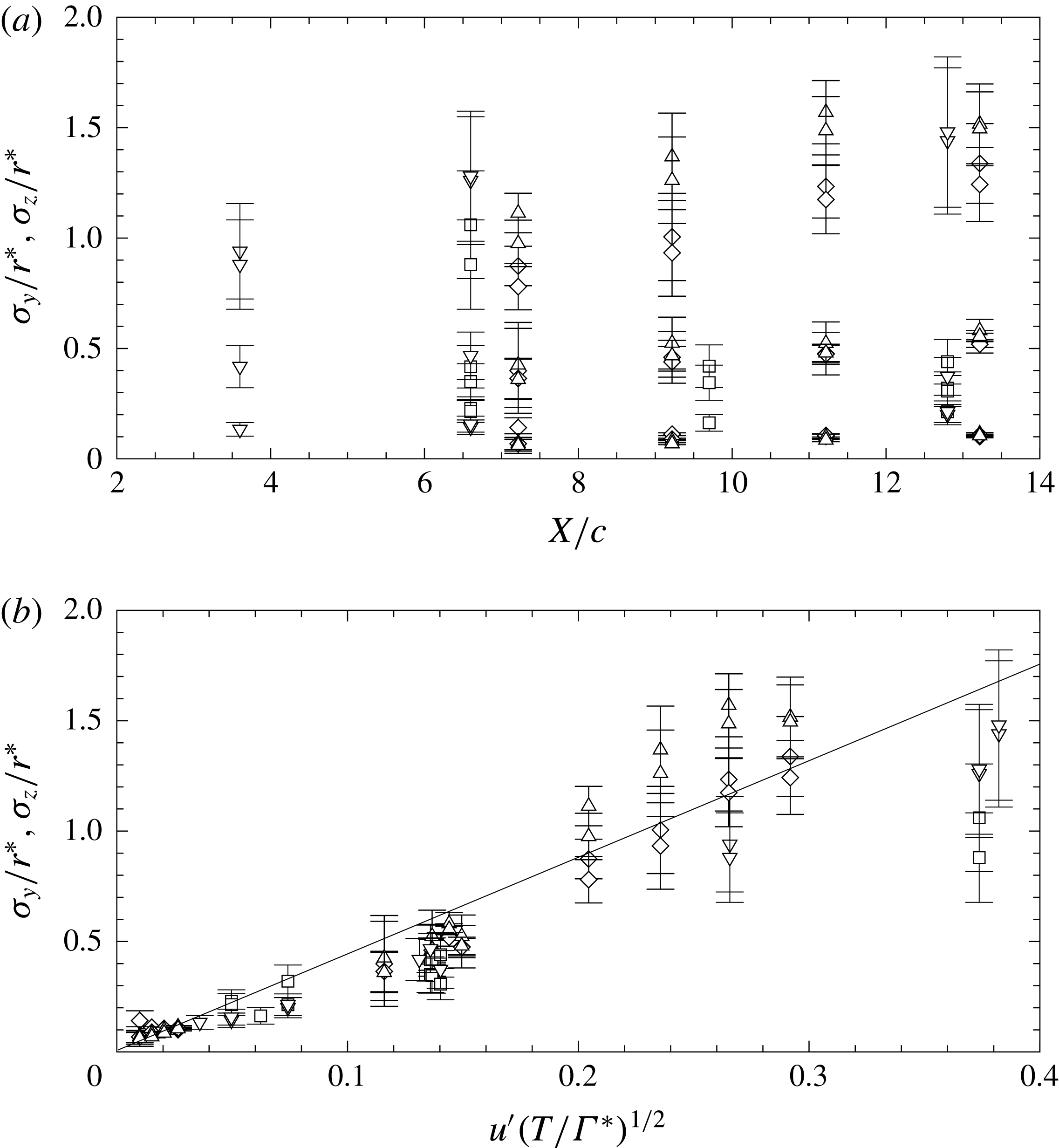
The wandering amplitudes determined from the different facilities and approaches are presented in figure 5(a) and it can be observed that the different free-stream conditions produced a fairly wide range of
 $\unicode[STIX]{x1D70E}_{y}$
and
 $\unicode[STIX]{x1D70E}_{z}$
at the same streamwise location. To compare and scale these results, it seems worthwhile to explore the approach of van Jaarsveld et al. (Reference van Jaarsveld, Holten, Elsenaar, Trieling and van Heijst2011), which was mentioned in § 1 and is presented in figure 5(b). This scaling method assumes that vortex wandering is analogous to the dispersion of a passive scalar injected from a point source in homogeneous turbulence. Taylor’s theory of passive scalar diffusion uses the Lagrangian time scale of the turbulence as an important parameter; van Jaarsveld et al. substituted this scale by the turnover time of the vortex, approximated as
 $T_{to}=2\unicode[STIX]{x03C0}r^{\ast }/U^{\ast }$
, as a way to account for the interaction of the vortex and the free-stream turbulence, albeit plainly admitting that ‘there is no sound physical explanation’ for this substitution. Van Jaarsveld et al. thus derived the following expressions for the local normalised wandering amplitudes:
 $$\begin{eqnarray}\unicode[STIX]{x1D70E}_{y}/r^{\ast },\unicode[STIX]{x1D70E}_{z}/r^{\ast }\propto u^{\prime }(T/\unicode[STIX]{x1D6E4}^{\ast })^{1/2},\end{eqnarray}$$
where
 $u^{\prime }$
is the standard deviation of turbulence fluctuations,
 $\unicode[STIX]{x1D6E4}^{\ast }=2\unicode[STIX]{x03C0}r^{\ast }|U^{\ast }|$
is the core circulation and
 $T$
is the residence time of the vortex in the turbulence; for the present configurations, we may estimate these properties as
 $u^{\prime }\approx (2/3k)^{1/2}$
(
 $k$
is the local turbulent kinetic energy per unit mass) and
 $T\approx (X-3c/4)/U_{0}$
.
(a) Streamwise evolution of normalised wandering amplitudes for different free-stream turbulence conditions and (b) the same results plotted using scaling proposed by van Jaarsveld et al. (Reference van Jaarsveld, Holten, Elsenaar, Trieling and van Heijst2011). The solid line is (4.1) using
 $0.07+4.21u^{\prime }(T/\unicode[STIX]{x1D6E4}^{\ast })^{1/2}$
as determined by van Jaarsveld et al. (Reference van Jaarsveld, Holten, Elsenaar, Trieling and van Heijst2011) from a fit of their results; ▵ denotes estimates from the analysis of § 3.1; ♢ denotes estimates by Bailey & Tavoularis (Reference Bailey and Tavoularis2008); ▫ denotes estimates from water tunnel LIF; ▿ are from water tunnel PIV. Uncertainty bars for the § 3.1 analysis were determined from variation between results for different
 $\unicode[STIX]{x0394}S$
. Uncertainty bars for the water tunnel results are based on per cent difference between the PIV and LIF estimates at overlapping conditions.

Some caution is necessary when applying the van Jaarsveld et al. scaling postulate to the present results, because, like Taylor’s diffusion theory, it applies to strictly homogeneous turbulence and not necessarily to grid turbulence, which decays with streamwise distance. Equation (4.1) leads to the paradoxical predictions that wandering would vanish when turbulence vanishes, even if it occurred at some upstream location, and that if turbulence were introduced at some intermediate location in the vortex path, finite-amplitude wandering would be enforced in a stepwise manner. These paradoxes could be resolved, at least in part, if local wandering were not scaled by local turbulence conditions but by scales that take into account the history of wandering motion. One may also postulate that, when turbulence and free-stream unsteadiness drop below a certain level, vortex wandering would persist as the result of intrinsic instabilities; equation (4.1) cannot be expected to hold under such conditions.
In any case, such problems do not apply to the present conditions, as we found good agreement between the values of
 $\unicode[STIX]{x1D70E}_{y}$
and
 $\unicode[STIX]{x1D70E}_{z}$
calculated from the components of
 $\boldsymbol{r}_{v}(t)$
, the same properties obtained with the use of a single-probe signal analysis by Bailey & Tavoularis (Reference Bailey and Tavoularis2008), the values determined from the water tunnel study, which were at a Reynolds number that was an order of magnitude lower than that in the wind tunnel tests, and the values determined from the measurements of van Jaarsveld et al. (which are summarised by the solid line in figure 5
b). Although the apparent scatter of the wandering amplitudes is slightly larger for the large-grid case, it is within the estimated uncertainty and in remarkably good agreement with the no-grid and small-grid cases. Such agreement provides support for van Jaarsveld et al.’s observation that the vortex turnover time is an important scaling parameter for the wandering amplitude.
Most importantly, the fair agreement between wandering amplitudes measured in two very different facilities, at two distant Reynolds numbers and six different free-stream conditions, and with the use of three different experimental techniques (hot-wire anemometry, LIF flow visualisation and SPIV) and five different data processing algorithms provides confidence in the analysis presented in § 3.1 and suggests that the wandering amplitude depends entirely on the kinetic energy of the turbulence and is insensitive to its integral length and time scales. The insensitivity to the relative size of dominant turbulence eddies (presumed to be proportional to the grid mesh size) can be clearly demonstrated by comparing the present wind tunnel results with the small and large grids and those by van Jaarsveld et al. Normalised by the grid mesh size, the corresponding vortex core sizes for these three cases were
 $r^{\ast }/M\approx 0.28$
, 0.14 and 0.05, nearly spanning an order of magnitude of values, but these differences do not appear to have any measurable effect on the normalised wandering amplitude.
4.2 Wandering frequency and wavelength
Most previous experimental investigations of vortex wandering induced by free-stream turbulence focused on the amplitude of wandering (Devenport, Zsolodos & Vogel Reference Devenport, Zsolodos and Vogel1997; Heyes et al. Reference Heyes, Jones and Smith2004; Bailey & Tavoularis Reference Bailey and Tavoularis2008; Beresh et al. Reference Beresh, Henfling and Spillers2010; van Jaarsveld et al. Reference van Jaarsveld, Holten, Elsenaar, Trieling and van Heijst2011), under the presumption that such wandering would be stochastic. There seems to be a general agreement that the meandering of the vortex has a relatively long wavelength, but little documentation of the actual wavelength or frequency of wandering. Our present reconstruction of the time series of vortex position in § 3.1, combined with analysis of the LIF imagery, provide us an opportunity to estimate both the wavelength and the frequency of wandering.
To examine the frequency
 $f$
of wandering, we computed the frequency spectra
 $\unicode[STIX]{x1D719}_{yy}(f)$
and
 $\unicode[STIX]{x1D719}_{zz}(f)$
of the
 $y$
and
 $z$
components of the
 $\boldsymbol{r}_{v}(t)$
time series; by definition of these spectra,
 $\unicode[STIX]{x1D70E}_{y}^{2}=\int _{0}^{\infty }\unicode[STIX]{x1D719}_{yy}\,\text{d}f$
and
 $\unicode[STIX]{x1D70E}_{z}^{2}=\int _{0}^{\infty }\unicode[STIX]{x1D719}_{zz}\,\text{d}f$
. The two types of spectra were virtually identical, so we will only discuss the
 $\unicode[STIX]{x1D719}_{yy}(f)$
estimates.
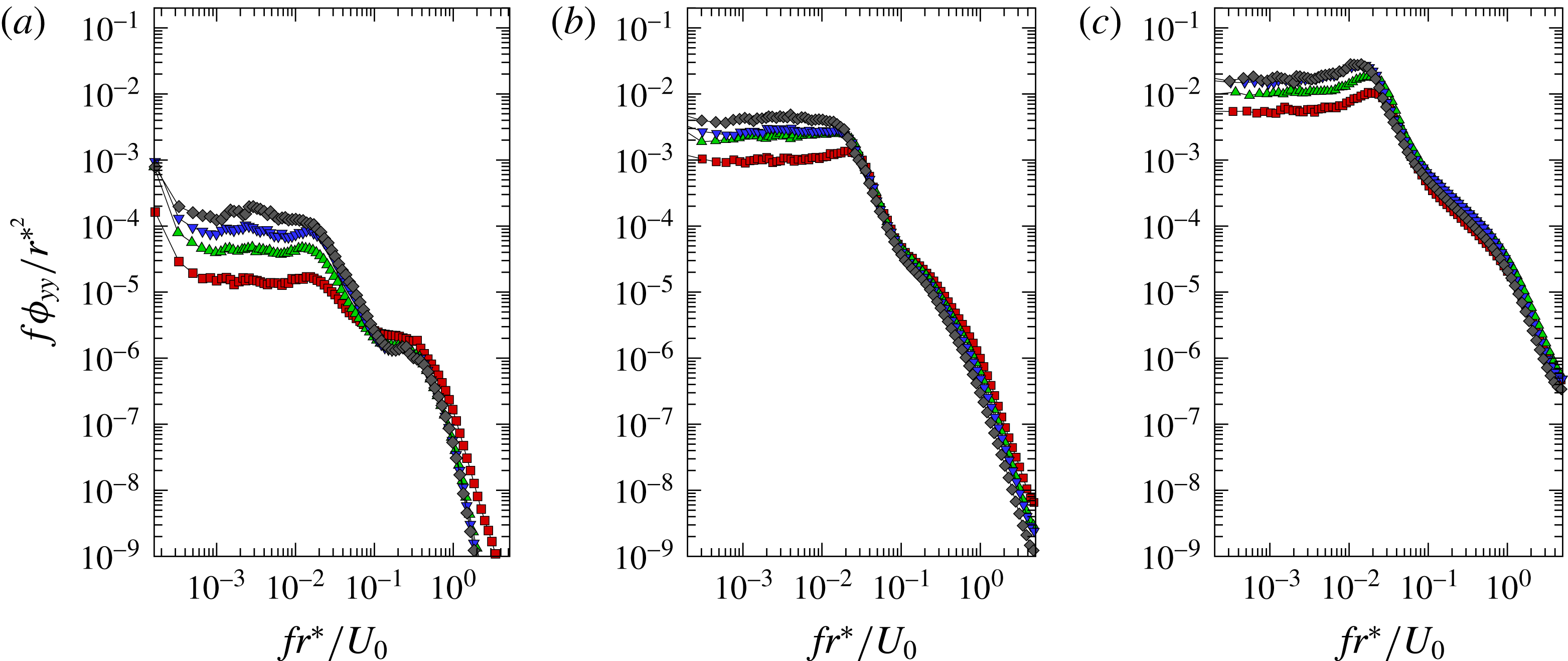
The ensemble-averaged frequency spectra determined for the no-grid, small-grid and large-grid cases are provided in figures 6(a) to 6(c) respectively, scaled by the core radius. The no-grid case is shown in figure 6(a) and is characterised by relatively constant
 $\unicode[STIX]{x1D719}_{yy}$
to
 $fr^{\ast }/U_{0}\approx 0.02$
, after which there is a decay to
 $fr^{\ast }/U_{0}\approx 0.2$
, at which frequency a shoulder appears. At higher frequencies
 $\unicode[STIX]{x1D719}_{yy}$
decays monotonically. Most of the increase in wandering amplitude with streamwise distance appears to come from the lower frequencies,
 $fr^{\ast }/U_{0}<0.2$
. Similar behaviour can be observed in the spectra measured from the small- and large-grid cases, although the shoulder is much less pronounced for the cases with free-stream turbulence, and there is a broadband hump in the spectra around
 $fr^{\ast }/U_{0}\approx 0.1$
to 0.2 which appears in the spectra measured closest to the wing in the small-grid case, and at all streamwise locations of the large-grid case.
Frequency spectra of
 $y_{v}$
for (a) no-grid, (b) small-grid and (c) large-grid cases. Symbols indicate measurement location: ▫
 $X/c=3.75$
; ▵
 $X/c=5.75$
; ▿
 $X/c=7.75$
; ♢
 $X/c=9.75$
.

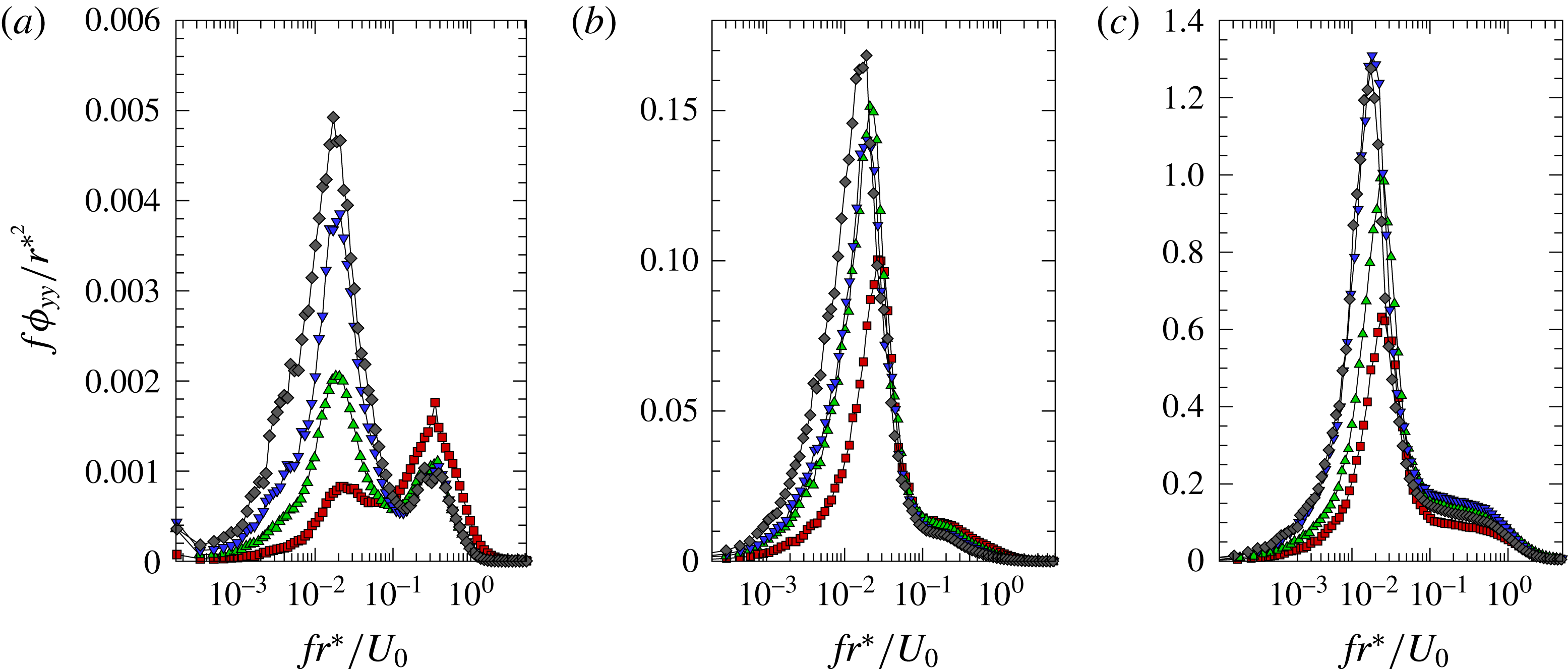
Further insight into these spectra can be gained by viewing them in pre-multiplied form. Pre-multiplied, ensemble-averaged spectra scaled by the core radius
 $f\unicode[STIX]{x1D719}_{yy}(f)/r^{\ast 2}$
for the no-grid, small-grid and large-grid cases are plotted in figure 7 versus the logarithm of the dimensionless frequency. With this choice of axes, the ‘relative energies’ (namely, the portions of
 $\unicode[STIX]{x1D70E}_{y}^{2}$
) within different frequency bands can be easily compared, as each is proportional to the area under the curve within that band. The frequency spectra also identify the most probable frequencies of wandering as the frequencies of the spectral peaks. It must be noted, however, that the probability that any specific frequency, including a most probable one, will ever occur is zero and probabilities can only be assigned to finite frequency bands. Each wandering frequency value corresponds to a wavelength of wandering motion of the vortex axis, under the assumption that the vortex is convected past the probe by the free-stream velocity
 $U_{0}$
; thus, the axis position wavelength that corresponds to a certain frequency of wandering can be estimated as
 $\unicode[STIX]{x1D706}\approx U_{0}/f$
.
A general observation that applies to all plots in figure 7 is that wandering energy was spread over approximately three orders of magnitudes of frequency. This clearly illustrates that, in all cases, wandering was largely stochastic and was composed of motions with very different scales. Although all spectra had well-defined peaks at one or two most probable frequencies, the relative energy within a band that was within 50 % of the peak frequency was in all cases but a very small fraction of the total energy. This proves that motions with frequencies at or near the most probable values were rare.
The same spectra as figure 6 shown in pre-multiplied form for (a) no-grid, (b) small-grid and (c) large-grid cases. Symbols indicate measurement location: ▫
 $X/c=3.75$
; ▵
 $X/c=5.75$
; ▿
 $X/c=7.75$
; ♢
 $X/c=9.75$
. Note: vertical axis scales are not the same for panels (a–c).

The frequency spectra at all streamwise locations of the no-grid case, shown in figure 7(a), exhibit two distinct, and relatively broad, bands, each centred about a strong peak. One band corresponds to relatively long wavelengths (
 $10r^{\ast }<\unicode[STIX]{x1D706}<1000r^{\ast }$
) and another corresponds to relatively short wavelengths (
 $r^{\ast }<\unicode[STIX]{x1D706}<10r^{\ast }$
). Near the wing (
 $X/c=3.75$
), motions within each of the two bands accounted for roughly half of
 $\unicode[STIX]{x1D70E}_{y}^{2}$
, but, as the vortex was convected downstream, the energy of the short-wavelength band decayed, whereas the energy of the long-wavelength band increased; as a result, at the last measuring station (
 $X/c=9.75$
) the long-wavelength band contributed 80 % of the wandering motion. These observations indicate that short-wavelength wandering motions likely received some initial energy from an upstream source, possibly near the wing or even further upstream, but lacked a mechanism capable of maintaining their energy and were dissipated by viscous actions. In contrast, long-wavelength motions were not dissipated with travel along the test section.
One may argue that short-wavelength wandering could be an artefact of the trajectory reconstruction process and a residual of conditions during vortex formation, which were specific to our set-up. Nevertheless, short-wavelength modes have also been observed previously under different conditions. For example, transient growth analysis has predicted an increased amplification of disturbances for streamwise wavenumbers around
 $k=1.4$
, which corresponds to a wavelength of approximately
 $5r^{\ast }$
or
 $fr^{\ast }/U_{0}\approx 0.2$
(Antkowiak & Brancher Reference Antkowiak and Brancher2004). Moreover, our observation that the energy of short-wavelength motions decayed downstream is consistent with the observations of Hussain et al. (Reference Hussain, Pradeep and Stout2011). It seems plausible that short-wavelength wandering was induced by residual turbulence and secondary structures originating at the wing.
The frequency spectra for the small- and large-grid cases (figures 7
b and 7
c, respectively) had values that were, respectively, one and two orders of magnitude larger than corresponding no-grid spectra. The shapes of the small- and large-grid spectra were consistent with each other but quite different from the no-grid spectra. In both cases with grids, and at all streamwise stations, there was a single spectral peak, surrounded by a relatively wide long-wavelength band. Although no peak was visible at relatively high frequencies, the spectra were somewhat elevated in a high-frequency spectral band, which indicates that some energy of short-wavelength motions persisted through grid turbulence. As this energy was relatively small (it varied from
 $0.2\unicode[STIX]{x1D70E}_{y}^{2}$
near the wing to
 $0.05\unicode[STIX]{x1D70E}_{y}^{2}$
far downstream), we will not discuss it any further, but will accept that grid turbulence essentially obliterated any short-wavelength motions that were introduced at or upstream of the wing. Turning again to the long-wavelength motions, we can make two observations. First, unlike the no-grid case, the energy of such motions increased monotonically with streamwise distance, with the rate of increase being significantly higher for the large-grid than the small-grid case. Second, as the vortex travelled downstream, the spectral peak kept shifting towards lower frequencies, whereas for the no-grid case the spectral peak was at a constant frequency, which means that the most probable wavelength of wandering tended to increase.
Having established that free-stream turbulence has a strong influence on vortex wandering, it seems worthwhile to explore any possible relationship between the wandering wavelength and the scales of turbulence. The integral length scale of the turbulence, which is a measure of the size of the energy containing eddies, was
 $L_{x}\approx 5r^{\ast }$
(Bailey & Tavoularis Reference Bailey and Tavoularis2008); this is an order of magnitude smaller than the most probable wavelength of wandering (
 ${\approx}50r^{\ast }$
) and so
 $L_{x}$
can be excluded as a possible scale of the wandering motion. Another relevant length scale of the turbulence would be the travelling distance
 $U_{0}L_{x}/u^{\prime }$
of a dominant eddy during its typical lifetime (eddy turnover time)
 $L_{x}/u^{\prime }$
; this distance was in the range from
 $100r^{\ast }$
to
 $200r^{\ast }$
for the cases shown in figure 7, which is rather too large compared to the most probable wandering wavelength. In conclusion, the wavelength of wandering does not seem to be connected to a length scale of the free-stream turbulence.
Previous authors suggested that bending waves can be induced into the vortex by vortical coherent structures in the free-stream turbulence through a transient growth of perturbations (Pradeep & Hussain Reference Pradeep and Hussain2006; Hussain et al.
Reference Hussain, Pradeep and Stout2011), which tend to get wrapped around the vortex and form azimuthally aligned secondary vortices (Melander & Hussain Reference Melander and Hussain1993; Marshall & Beninati Reference Marshall and Beninati2005; Takahashi et al.
Reference Takahashi, Ishii and Miyazaki2005). Such secondary vortices were observed in our flow visualisation images (see examples in figure 3); their streamwise separation was between
 $2r^{\ast }$
and
 $6r^{\ast }$
, which is consistent with past observations (Marshall & Beninati Reference Marshall and Beninati2005). As noted previously, the scale of these structures is consistent with short-wavelength wandering, but too small to trigger long-wavelength wandering. This conjecture is consistent with the vortex appearance in figure 3(c), which shows that the amplitude of short-wavelength bending was much smaller than that of long-wavelength bending, even though short-wavelength bending in figure 3(c) was more intense than in figure 3(a,b) that correspond to flows with lower turbulence. In conclusion, the action of vortices from the free stream can make at most a small contribution to the overall wandering motion of the main vortex.
One potential source of long-wavelength motions is the transient growth mechanism, which was previously connected to short-wavelength motions. Long-wavelength modes are also excited by this mechanism, with the energy growth increasing with decreasing wavelength (as observed by Fontane et al. Reference Fontane, Brancher and Fabre2008, for example). However, the optimal time for such motions to develop also increases with decreasing wavelength. Such motions would not likely have sufficient time to develop within the time frame examined in the current study, which encompassed fewer than 15 vortex rotation periods. This postulate is supported by the lack of energy amplification at long wavelengths in the observations of Hussain et al. (Reference Hussain, Pradeep and Stout2011), who studied a vortex in the presence of decaying turbulence; a possible explanation of this phenomenon is that the turbulent perturbations decayed faster than the time required for the long-wavelength motions to be excited and attain a detectable amplitude. In summary, considering that the turbulence in our tests was decaying and the measurable vortex was relatively young, it is unlikely that the observed long-wavelength wandering motions would be caused by transient growth.
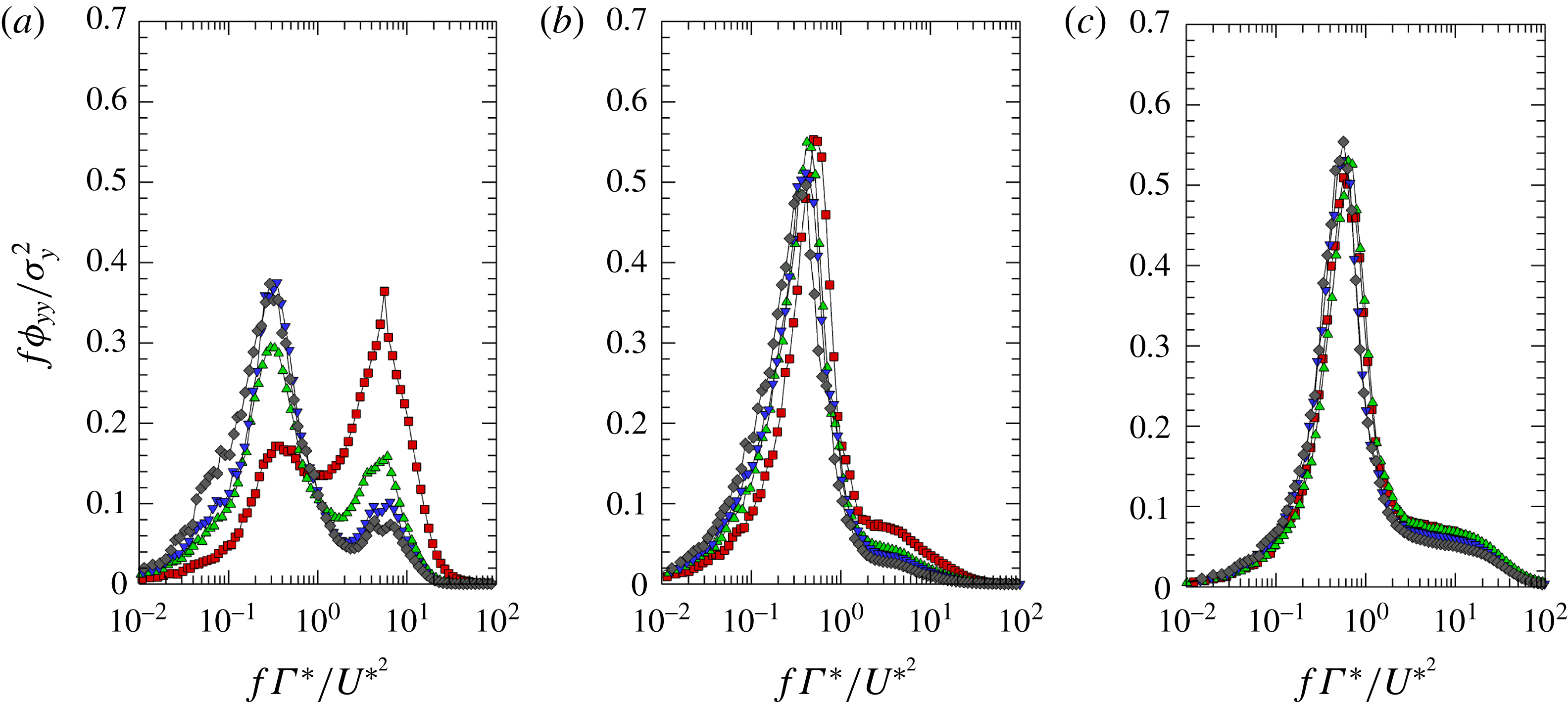
Pre-multiplied frequency spectra of
 $y_{v}$
for (a) no-grid, (b) small-grid and (c) large-grid cases with the frequency scaled by vortex turnover time and the vertical axis normalised by wandering amplitude. Symbols indicate measurement location: ▫
 $X/c=3.75$
; ▵
 $X/c=5.75$
; ▿
 $X/c=7.75$
; ♢
 $X/c=9.75$
.

We now turn to examining the possible connection of long-wavelength motions to intrinsic scales of the vortex. As mentioned in § 4.1, an intrinsic time scale of the vortex is its turnover time
 $T_{to}=2\unicode[STIX]{x03C0}r^{\ast }/U^{\ast }=\unicode[STIX]{x1D6E4}^{\ast }/U^{\ast 2}$
; in the present wind tunnel experiments, this varied from approximately 0.006 to 0.010 s. When we normalised the frequency by the turnover time and the spectra by
 $\unicode[STIX]{x1D70E}_{y}^{2}$
(figure 8), we observed that the spectral peaks in the two cases with grids essentially collapsed; in the no-grid case, the locations of the low-frequency peaks also collapsed, but the spectral shapes at different streamwise locations differed significantly because of the contributions of short-wavelength motions. The period of wandering
 $T_{p}=1/f_{P}$
, corresponding to the frequency
 $f_{p}$
of the spectral peak, was in all cases
 $T_{p}\approx 2T_{to}$
; spectral bands with significant energy around the low-frequency peak corresponded to periods in the range from 1 to
 $10T_{to}$
.
An estimate of the dimensionless average wavelength of the wandering vortex axis, under the assumption that the vortex is approximately convected downstream by the free-stream velocity
 $U_{0}$
, can be obtained as
 $\unicode[STIX]{x1D706}_{p}/r^{\ast }\approx U_{0}T_{p}/r^{\ast }\approx 2U_{0}T_{to}/r^{\ast }=4\unicode[STIX]{x03C0}U_{0}/U^{\ast }$
. The value of
 $\unicode[STIX]{x1D706}_{p}/r^{\ast }$
varied roughly from 30 to 60, depending on the free-stream conditions and the streamwise location. In the absence of direct measurements of
 $\unicode[STIX]{x1D706}$
, we cannot test our hypothesis that this scaling is appropriate for the wind tunnel data. Such a test can, however, be performed for the water tunnel data, because in these cases the wavelength
 $\unicode[STIX]{x1D706}$
of the instantaneous vortex axis was determined directly by inspection of reconstructed three-dimensional flow visualisation images (§ 3.2). The relatively low resolution of our visual approach did not allow us to determine a precise value of
 $\unicode[STIX]{x1D706}$
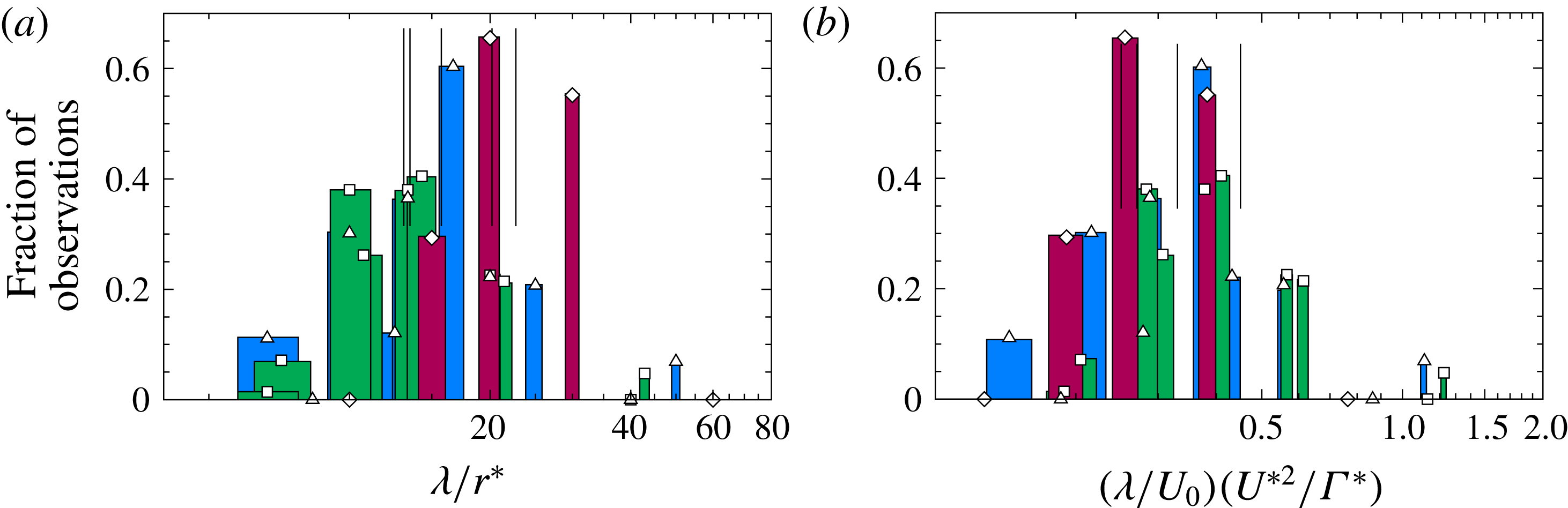
for each pair of images; instead, we classified each roughly estimated value in one of five different bins, assigned to represent waveforms with quarter, half, three-quarter, one and one-and-a-quarter full waves. Histograms of the observed wavelengths, normalised by
 $r^{\ast }$
, for the three free-stream conditions are shown in figure 9(a). In all cases, irrespective of turbulence conditions and distance downstream of the wing, the average detected wavelength was comparable to the length of the images that were considered. Although it is theoretically possible that a consideration of longer images would have resulted in a longer average wavelength, the statistical distribution of the present results does not support this conjecture. Furthermore, all estimates of
 $\unicode[STIX]{x1D706}$
in the water tunnel studies were in the range
 $\unicode[STIX]{x1D706}/r^{\ast }\leqslant 50$
, which is within the range of the wind tunnel estimates of this parameter. A comparison of the results shown in figure 9(a) for the three free-stream cases revealed that the ranges of values of
 $\unicode[STIX]{x1D706}/r^{\ast }$
shifted towards the right of the axis as the turbulent intensity was increased. This indicates that
 $r^{\ast }$
is not an appropriate scale by which to normalise the measured
 $\unicode[STIX]{x1D706}$
. When, however, we normalised
 $\unicode[STIX]{x1D706}$
by
 $U_{0}T_{to}$
(figure 9
b), we found that the ranges of the three sets of data collapsed (at least within the relatively large uncertainty of these estimates). In summary, we can assert with some confidence that the wandering wavelength is proportional to the vortex turnover time.
Histograms of wandering wavelengths in the water tunnel studies, determined from analysis of LIF images and scaled by core radius (a) and by vortex turnover time (b), for the no-grid (▫), small-grid (▵) and large-grid (♢) cases.

4.3 Vortex wandering velocity
To gain further insight into long-wavelength wandering, we calculated the part of the Lagrangian velocity of the vortex axis that corresponds to this spectral band. This velocity was estimated from the low-pass filtered time series
 $\boldsymbol{r}_{vf}$
of vortex axis position as
 $\text{d}\boldsymbol{r}_{vf}/\text{d}t$
. A fourth-order Butterworth, low-pass filter having 3 dB cutoff setting at
 $fr^{\ast }/U_{0}=0.05$
was used to reduce effects of short-wavelength wandering and random noise generated by the time series reconstruction process. First, the Cartesian components of the Lagrangian velocity were calculated as
 $V_{y}=\text{d}y_{vf}/\text{d}t$
and
 $V_{z}=\text{d}z_{vf}/\text{d}t$
with the use of a second-order central differencing scheme and then the time series of radial and circumferential components of this velocity were determined, respectively, as
 $$\begin{eqnarray}\displaystyle V_{r}(r,\unicode[STIX]{x1D703},t)=V_{y}(r,\unicode[STIX]{x1D703},t)\cos \unicode[STIX]{x1D703}+V_{z}(r,\unicode[STIX]{x1D703},t)\sin \unicode[STIX]{x1D703} & & \displaystyle\end{eqnarray}$$
and
 $$\begin{eqnarray}\displaystyle V_{\unicode[STIX]{x1D703}}(r,\unicode[STIX]{x1D703},t)=V_{z}(r,\unicode[STIX]{x1D703},t)\cos \unicode[STIX]{x1D703}-V_{y}(r,\unicode[STIX]{x1D703},t)\sin \unicode[STIX]{x1D703}, & & \displaystyle\end{eqnarray}$$
where
 $\unicode[STIX]{x1D703}=\tan ^{-1}z_{vf}/y_{vf}$
and
 $r^{2}=z_{vf}^{2}+y_{vf}^{2}$
.
Ensemble-averaged probability density functions of
 $V_{r}$
for the (a) no-grid, (b) small-grid and (c) large-grid cases. Also shown are the probability density functions of
 $V_{\unicode[STIX]{x1D703}}$
for the (d) no-grid, (e) small-grid and (f) large-grid cases. Symbols indicate measurement location: ▫
 $X/c=3.75$
; ▵
 $X/c=5.75$
; ▿
 $X/c=7.75$
; ♢
 $X/c=9.75$
.

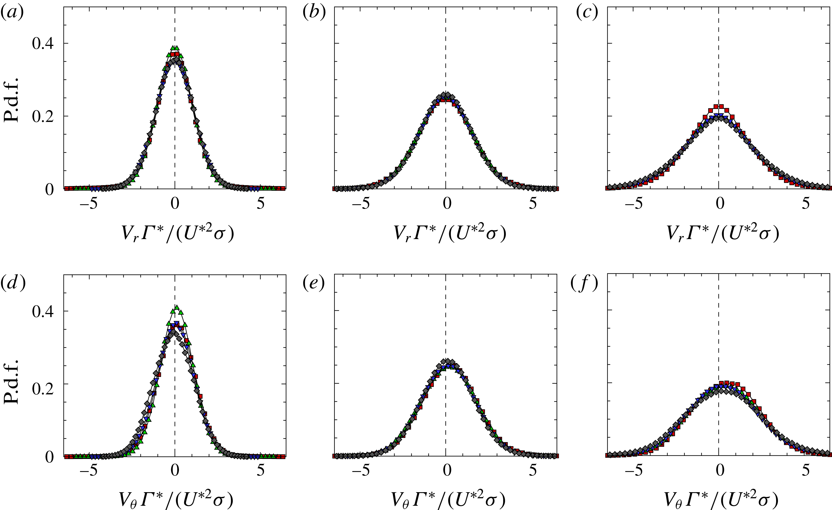
The ensemble-averaged probability density functions (p.d.f.s) of
 $V_{r}$
and
 $V_{\unicode[STIX]{x1D703}}$
for the no-grid, small-grid and large-grid cases are shown in figure 10. A scale for normalising these velocities was devised as
 $U^{\ast 2}\unicode[STIX]{x1D70E}/\unicode[STIX]{x1D6E4}^{\ast }$
by assuming that, during a vortex turnover time
 $\unicode[STIX]{x1D6E4}^{\ast }/U^{\ast 2}$
, the vortex would shift transversely by a distance that would be proportional to the average wandering amplitude
 $\unicode[STIX]{x1D70E}=(\unicode[STIX]{x1D70E}_{y}^{2}+\unicode[STIX]{x1D70E}_{z}^{2})^{1/2}$
. All p.d.f.s were nearly Gaussian, having skewnesses in the range
 $\pm 0.1$
and flatnesses in the range from 2.9 to 3.4, except close to the wing, where wake effects were more significant. This Gaussian behaviour enforces an interpretation that the wandering was largely stochastic. There is, however, a noticeable difference between the p.d.f.s of the two velocity components. Whereas the mean
 $V_{r}$
was essentially zero (actually, in the range
 $\pm 0.001~\text{m}~\text{s}^{-1}$
) in all cases, the mean
 $V_{\unicode[STIX]{x1D703}}$
was measurably positive (approximately
 $0.01~\text{m}~\text{s}^{-1}$
for the no-grid,
 $0.1~\text{m}~\text{s}^{-1}$
for the small-grid and
 $0.5~\text{m}~\text{s}^{-1}$
for the large-grid cases). Combined with the streamwise translation of the vortex by approximately the free-stream velocity, the positive circumferential velocity of the vortex axis indicates that, on average, the vortex was in clockwise helical motion along a path around the time-averaged vortex axis when facing in the streamwise direction. The increase of the average
 $V_{\unicode[STIX]{x1D703}}$
from the no-grid to the small-grid cases and further to the large-grid case also indicates that the angular velocity of this helical motion increased with increasing turbulence intensity.
It is very important to emphasise that the presence of a helical motion was only detectable as an average of very disparate types of wandering motions. This becomes apparent if one considers that the average
 $V_{\unicode[STIX]{x1D703}}$
was less than 25 % of its standard deviation at
 $X/c=3.75$
and decreased to less than 15 % at
 $X/c=9.75$
. The rareness of occurrence of helical motions is further obviated by the fact that the probability of
 $V_{\unicode[STIX]{x1D703}}$
values in a range within 50 % of the mean was but a very small per cent of the total probability for all three free-stream conditions (figure 10
d–f). In fact, the probability of any clockwise vortex rotation was only slightly higher than that of any anticlockwise rotation.
Consistent with stochastic wandering, figure 10 further shows that the p.d.f.s of the normalised radial velocity for each of the three free-stream conditions essentially collapsed at all streamwise locations; the same observation applies to the circumferential velocity. Based on these observations, it appears that the choice of
 $U^{\ast 2}\unicode[STIX]{x1D70E}/\unicode[STIX]{x1D6E4}^{\ast }$
as velocity scale was appropriate for scaling the stochastic axis motion of a vortex subjected to specific free-stream turbulence. The rationale for this choice will be discussed in § 5.
It has been well established in the literature that wavelengths with an azimuthal wavenumber of unity (
 $|m|=1$
) are subject to transient amplification (Antkowiak & Brancher Reference Antkowiak and Brancher2004) and can contribute to wandering (Edstrand et al.
Reference Edstrand, Davis, Schmid, Taira and Cattafesta2016). One of the more dominant long-wavelength
 $|m|=1$
modes is Kelvin bending waves, also referred to as displacement waves (Fabre et al.
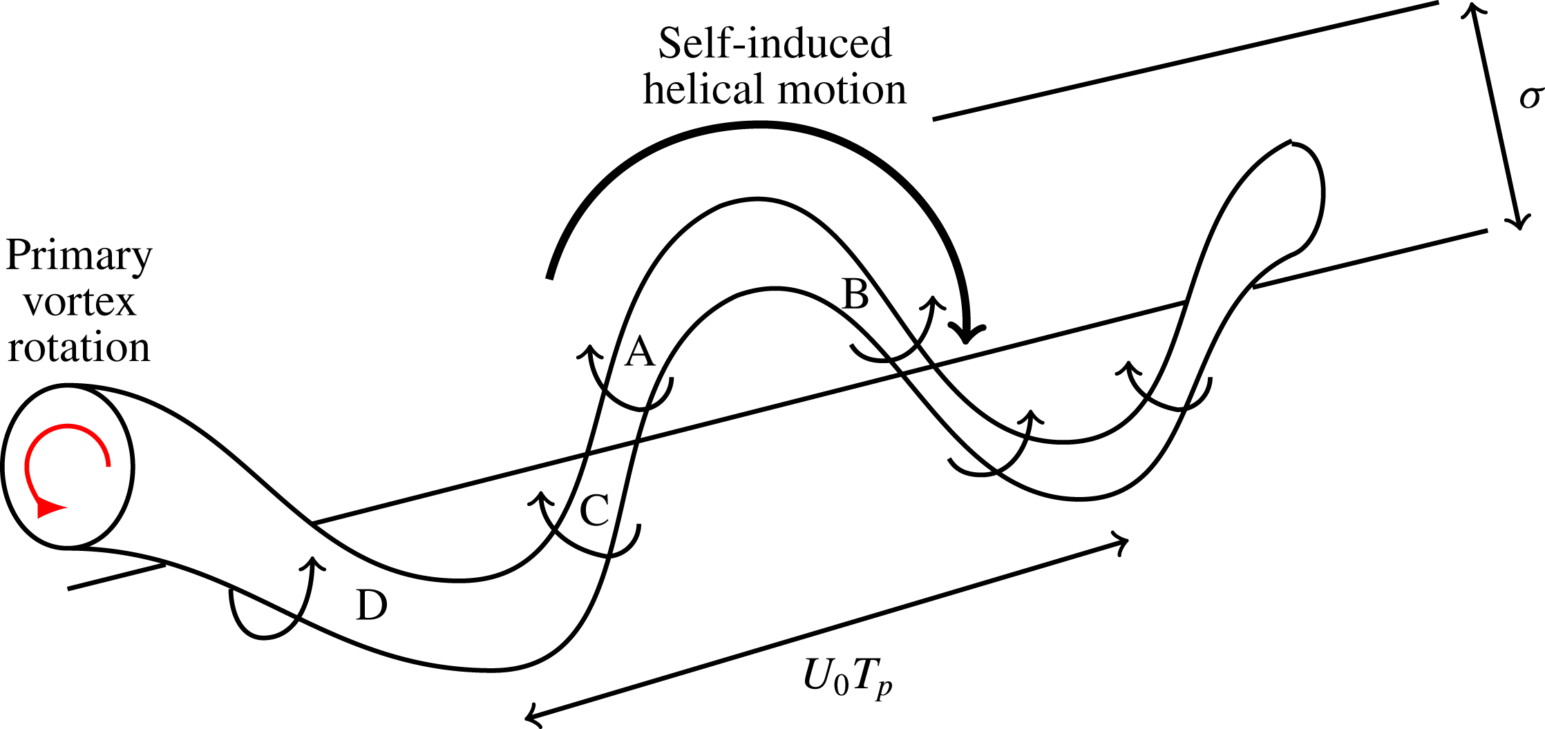
Reference Fabre, Sipp and Jacquin2006), which may introduce a helical motion via Biot–Savart induction (Kelvin Reference Kelvin1880; Widnall Reference Widnall1975; Saffman Reference Saffman1995). This self-induced rotation can be explained qualitatively with the help of the sketch in figure 11. Assume that, as the result of interactions with free-stream turbulence, the vortex axis has a planar, quasi-sinusoidal shape. By the law of Biot–Savart, each segment of the vortex would be subjected to the velocity field induced by any other segment, but it is the closest segments that have the strongest influence. Therefore, segment A, i.e. the upper half of the left side of the wave in figure 11, would be mainly under the influence of the field induced by the neighbouring segment B, as segment C (the lower half of the left side of the wave) is nearly coaxial with segment A and has negligible effect on it. It is easy to see that segment A would tend to move out of the plane of the illustration under the influence of segment B. Similarly, segment B would also tend to move out of the plane under the influence of segment A. Conversely, segment C would tend to move into the plane under the influence of segment D. In summary, the entire vortex would be set in self-induced clockwise rotation in a preferential direction, which combined with streamwise transport by the free stream, would generate the observed clockwise helical motion of the axis.
Sketch illustrating the self-induced rotation of the vortex under the influence of a bending wave.

We now proceed to devise a scale for the angular velocity of the helical motion of the vortex under the assumption that this motion is self-induced. As reviewed in Alekseenko, Kuibin & Okulov (Reference Alekseenko, Kuibin and Okulov2007), a helical vortex filament with a pitch that is much larger than its amplitude would be set in solid-body rotation with the same angular velocity as a plain sinusoidal vortex filament with the same wavelength (pitch) and amplitude as the helical filament. We approximate the influence of a perturbation on a filament of circulation
 $\unicode[STIX]{x1D6E4}^{\ast }$
by assuming that it introduces approximately sinusoidal deformation with amplitude
 $\unicode[STIX]{x1D70E}$
and a wavelength
 $\unicode[STIX]{x1D706}_{P}\approx U_{0}T_{p}$
. Then, following Alekseenko et al. (Reference Alekseenko, Kuibin and Okulov2007), one may calculate that the total induced velocity at the apices of this filament would be proportional to
 $\unicode[STIX]{x1D6E4}^{\ast }\unicode[STIX]{x1D70E}/\unicode[STIX]{x1D706}_{P}^{2}$
, which means that the angular velocity of this filament would be proportional to
 $\unicode[STIX]{x1D6E4}^{\ast }/\unicode[STIX]{x1D706}_{P}^{2}\approx \unicode[STIX]{x1D6E4}^{\ast }/(U_{0}^{2}T_{p}^{2})$
. The latter parameter would then be a plausible scale for the observed helical vortex rotation.
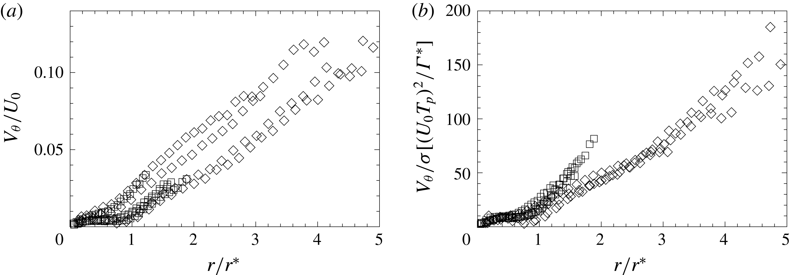
To test the appropriateness of this scale, we plot in figure 12 radial profiles of scaled, conditionally averaged
 $V_{\unicode[STIX]{x1D703}}$
. These profiles of
 $V_{\unicode[STIX]{x1D703}}$
were calculated by conditionally averaging
 $V_{\unicode[STIX]{x1D703}}(r,\unicode[STIX]{x1D703},t)$
by
 $r$
. To compare the effectiveness of scaling by the approximate angular velocity, the results are plotted normalised by
 $U_{0}$
in figure 12(a) and
 $\unicode[STIX]{x1D6E4}^{\ast }/(U_{0}^{2}T_{p}^{2})$
in figure 12(b). Conditional averaging of
 $V_{\unicode[STIX]{x1D703}}$
was done by classifying each instance of
 $V_{\unicode[STIX]{x1D703}}(r,\unicode[STIX]{x1D703},t)$
to one among 50 radially spaced bins in the range
 $0\leqslant r\leqslant 6\unicode[STIX]{x1D70E}$
, and then averaging all values within each bin for all
 $\unicode[STIX]{x0394}S$
. Because the scatter of these results increased significantly as the sample population decreased, we only considered results at radial bins for which 2000 or more values were averaged; unfortunately, this restricted the radial ranges of the results, particularly for the no-grid case, and for this reason we only present values for the small- and large-grid cases. Calculations similar to those for
 $V_{\unicode[STIX]{x1D703}}$
were also performed for the radial velocity, but will not be presented, as the average of this velocity was approximately zero at all radial positions. The radial variation of
 $V_{\unicode[STIX]{x1D703}}$
in figure 12 was roughly linear, which indicates that, in a frame convected with the free-stream velocity, the vortex axis was on average in nearly rigid-body rotation about its average position. Note that the scaling used in figure 12(b) assumes that the wavelength of the bending wave was constant, whereas, as illustrated in figure 7, motions with wavelengths within a broad range were present, which is considered to be the reason for the radial dependence of the induced angular velocity.
In consideration of the facts that the linear variation of the conditionally averaged
 $V_{\unicode[STIX]{x1D703}}$
extended well beyond
 $r^{\ast }$
and that
 $\unicode[STIX]{x1D70E}/r^{\ast }<1.5$
for all current free-stream turbulence conditions, we may assert that the (on average) rigid-body rotation of the axis covered the entire domain of its wandering. It is worthwhile to note that the angular velocity of this rigid-body rotation appeared to be sensitive to the free-stream conditions.
Circumferential velocity of the vortex axis, conditionally averaged based on radial position relative to the time-averaged vortex axis and normalised by (a) the free-stream velocity and (b) the ratio of circulation to wavelength; ▫ denotes small-grid cases and ♢ denotes large-grid cases.

The values in figure 12(b) for
 $r>r^{\ast }$
exhibited variations of approximately 10–20 %, which is approximately half the per cent variation of the unscaled
 $V_{\unicode[STIX]{x1D703}}/r$
. These results are subjected to considerable uncertainty, introduced by stochastic wandering motions, the roughness of assumptions and the small populations used for conditional averaging purposes. Differences in the scaling of the small- and large-grid cases may possibly be attributed to a weak dependence of the displacement wave instability on the properties of the vortex core (Fabre et al.
Reference Fabre, Sipp and Jacquin2006). Additional sources of uncertainty are the broadening of the range of perturbation amplitudes with an increase in turbulence intensity, which entails a broadening of the range of
 $V_{\unicode[STIX]{x1D703}}$
, and deviations of the wandering waveform from the sinusoidal shape, which would affect the distributions of
 $V_{r}$
and
 $V_{\unicode[STIX]{x1D703}}$
by self-induced motion. All things considered, however, we may view figure 12 as evidence that the entire vortex was, on average, in self-induced rotation, at least for the two cases with grids. It is equally important to re-iterate that the average
 $V_{\unicode[STIX]{x1D703}}$
was in all cases very small by comparison to the width of the range of observed instantaneous values of
 $V_{\unicode[STIX]{x1D703}}$
and so rigid-body rotation of any part of the vortex would be a rare event.
Helical motion should also produce correlation between the
 $y_{v}$
and
 $z_{v}$
components of vortex motion. However, we found this correlation to be relatively weak for the cases with free-stream turbulence with
 $\langle y_{v}z_{v}\rangle /(\unicode[STIX]{x1D70E}_{y}\unicode[STIX]{x1D70E}_{z})<0.1$
for these cases and closer to 0.05 for most of the measurements. In addition, if we assume that the hump observed in figure 6 for the grid cases can be attributed to this helical motion, we found that this hump contributed less than 10 % of the total variance for the two measurement locations nearest the wing for the small-grid case, and could not be observed for the two downstream locations. For the large-grid case, the hump in the spectra accounted for 20 % of the variance closest to the wing, but this contribution decreased to less than 15 % by the furthest downstream location. All these observations prove conclusively that the organised helical motion was only a small component of the overall wandering, which was largely stochastic.
In closing this section, it seems worthwhile to comment on the work of Edstrand et al. (Reference Edstrand, Davis, Schmid, Taira and Cattafesta2016), which also addressed vortex wandering. These authors examined experimentally one location of a vortex in a very low turbulence stream, conducted a linear stability analysis of a Batchelor vortex and concluded that vortex wandering is the result of an instability. In the absence of multiple data from which to attempt constructing scaling laws for the wandering frequency, they normalised it with the wing chord length and the free-stream velocity. A rough estimate of the Strouhal number
 $fc/U_{0}$
for the present experiments gives a value of about 0.45, which is of the same order as the value of about 0.1 in the work of Edstrand et al. (Reference Edstrand, Davis, Schmid, Taira and Cattafesta2016). Nevertheless, this is hardly evidence for the validity of this scaling postulate, but rather evidence of reproducibility of the organised motion, as the conditions in our wind tunnel experiments were not vastly different from those used by Edstrand et al. Both wings had the same profile and angle of attack, the chord of our wing was only 40 % shorter and our free-stream speed was only 23 % lower. It seems evident to us that this Strouhal number would be sensitive to the strength of the vortex, which would depend, among other factors, on the angle of attack. The opposite would imply that a symmetric airfoil at near-zero angle of attack would produce a vortex with the same wandering frequency as the one observed here! Finally, our observations and scaling of stochastic vortex wandering cannot be tested against the Edstrand et al.’s measurements, which were obtained in the absence of significant free-stream turbulence.
5 A physical justification of vortex turnover time as the scale of wandering frequency and amplitude
We have so far observed the presence of both short- and long-wavelength types of wandering. The long-wavelength motions had wavelengths in the range
 $10r^{\ast }<\unicode[STIX]{x1D706}<1000r^{\ast }$
and amplitudes that scaled with the vortex turnover time and were increased by a strengthening turbulence. The vortex axis velocity of long-wavelength motions was largely stochastic and also scaled with the vortex turnover time. We have also found evidence that, within the stochastic wandering, there was an azimuthal motion reminiscent of
 $|m|=1$
Kelvin bending waves that did not scale with the vortex turnover time. The azimuthal velocity of this organised motion was weak relative to the velocities of possible stochastic motions, as it only introduced a bias in
 $V_{\unicode[STIX]{x1D703}}$
that was very small compared to the range of observed
 $V_{\unicode[STIX]{x1D703}}$
values. We advanced the hypothesis that the organised motion was self-induced and the result of stochastic perturbations of the vortex axis by free-stream turbulence. In the remainder of this section we will provide some physical justification for our observation that the stochastic wandering scales with the vortex turnover time.
This scaling can be explained by considering that the stochastic wandering is the result of linear and angular momentum exchanges between the vortex and coherent structures (‘eddies’) from the free stream. In this analysis, we assumed that the strength of the primary vortex is much larger than that of any of the eddies, an assumption that applies well to the present experiments. When an eddy impacts the vortex, a portion of its linear momentum is transferred to the vortex, which tends to displace the vortex axis locally; at the same time, a portion of the angular momentum of the vortex is transferred to the eddy, which tends to wrap the eddy around the vortex, irrespective of the eddy orientation (Holzäpfel et al. Reference Holzäpfel, Hofbauer, Darracq, Moet, Garnier and Gago2003; Marshall & Beninati Reference Marshall and Beninati2005). The time scale of this interaction between the vortex and an individual eddy is set by the vortex rotation, as the momentum exchange must occur before the turbulent eddy deformation becomes so large that its coherence would be dissipated by viscous diffusion; moreover, the local interaction of the vortex with one eddy must be completed before its interaction with another eddy commences. Figure 13 shows schematically the interactions of the wingtip vortex with two turbulent eddies having different orientations. Regardless of eddy orientation, linear momentum exchange would occur mainly in a short time following impact and would be terminated within one vortex rotation, when the eddy would be completely wrapped around the vortex. During this time, the vortex would be shielded from other eddies that tend to approach it, and so the period of wandering would be insensitive to the subsequent eddy strength, size and time delay from the impact of the first eddy (i.e. the intensity and length scale of the free-stream turbulence). As the vortex gets convected downstream by the mean flow, it attains a quasi-sinusoidal appearance, with a long wavelength that separates transverse displacements caused by interactions with multiple eddies and occurring at a rate that is set by the vortex turnover time.
Wrapping of free-stream turbulent eddies around the wing-tip vortex: (a) perpendicular vortices and (b) parallel vortices.

6 Conclusions
The objective of this study was to identify and document the effects of free-stream turbulence on the wandering motion of a wing-tip vortex in the near field of the wing. Although numerous previous authors have addressed, and to some extent elucidated, various aspects of vortex wandering, there have been very few measurements of the wavelength and velocity of the wandering motion within free-stream turbulence. We obtained such measurements with the use of flow visualisation and an analysis technique which reconstructed the time series of vortex axis position from two-point, multi-component velocity measurements. These results were combined to provide a global view of the characteristics of vortex wandering in the presence of free-stream turbulence. Time series analysis indicated that an increase in free-stream turbulence intensity caused an increase in the amplitude of wandering, a result that is consistent with expectations and observations of previous authors. In accordance with the scaling law suggested by van Jaarsveld et al. (Reference van Jaarsveld, Holten, Elsenaar, Trieling and van Heijst2011), the vortex wandering amplitude was found to depend on the turbulence intensity and the vortex turnover time, namely the time required for the vortex to complete a rotation. This amplitude was insensitive to changes in the integral length and time scales of the turbulence.
The vortex turnover time was also found to be a suitable scale for the period of the vortex wandering and the tangential and radial velocities of the vortex axis. The prevalence of an inherent vortex time scale, rather than turbulence scales, on vortex wandering suggests that vortex-induced straining of the free-stream eddies bounds the interaction time between vortex and turbulence and, consequentially, limits the time available for momentum exchange between the two. The vortex motion was also found to contain a helical component, which was attributed to self-induced motion consistent with a long-wavelength displacement wave instability. The amplitude and rotational velocity of this coherent mode were found to increase with the increase in turbulence intensity.
In summary, we have demonstrated that the primary component of vortex wandering in a turbulent field is stochastic motions caused by impacting turbulent eddies, which interact with the vortex within a time that is set by the rate of rotation of the vortex. Because of this imposed scaling, the wandering wavelength is relatively long and has a finite range, and so the vortex waveform attains a shape amenable to self-induced rotation, which emerges as an average but rare mode of wandering.
Acknowledgement
Partial support for this work was provided by the Natural Sciences and Engineering Research Council of Canada.