1 Introduction
Scalar image velocimetry (SIV) is the reconstruction of the fluid velocity field
 $\boldsymbol{u}$
from measurements of a scalar field
 $\unicode[STIX]{x1D713}$
, that is advected by
 $\boldsymbol{u}$
. The technique is applied in weather forecasting models using e.g. satellite images of clouds or ocean temperature (see e.g. Kalnay Reference Kalnay2003). SIV also finds applications in medical flow imaging and in experimental fluid mechanics. For instance in the laser induced fluorescence (LIF) technique a fluid is seeded with fluorescent molecules and laser light is focused into a thin sheet, where it is absorbed by the fluorescent molecules followed by spontaneous emission of light which is recorded by a camera (see e.g. Su & Dahm Reference Su and Dahm1996). Assuming that the recorded light intensity is proportional to the fluorescence concentration
 $\unicode[STIX]{x1D713}$
, the velocity field
 $\boldsymbol{u}$
can be reconstructed by invoking the scalar transport equation:
 $\unicode[STIX]{x2202}_{t}\unicode[STIX]{x1D713}+\unicode[STIX]{x1D735}\boldsymbol{\cdot }(\boldsymbol{u}\unicode[STIX]{x1D713})-\unicode[STIX]{x1D706}\unicode[STIX]{x1D6FB}^{2}\unicode[STIX]{x1D713}=0$
, where
 $\unicode[STIX]{x1D706}$
is the scalar diffusivity. A direct inversion of the scalar transport equation only provides the component of
 $\boldsymbol{u}$
that is normal to
 $\unicode[STIX]{x1D713}$
isolines:
 $\boldsymbol{u}^{\bot }=(-\unicode[STIX]{x2202}_{t}\unicode[STIX]{x1D713}+\unicode[STIX]{x1D706}\unicode[STIX]{x1D6FB}^{2}\unicode[STIX]{x1D713})\unicode[STIX]{x1D735}\unicode[STIX]{x1D713}/|\unicode[STIX]{x1D735}\unicode[STIX]{x1D713}|^{2}$
. Finding all components of
 $\boldsymbol{u}$
requires additional constraints, e.g. conservation of hydrodynamic variables. These constraints are naturally implemented using a variational technique, involving a minimisation of a cost functional
 ${\mathcal{J}}$
. Previous works have used the following cost functional, which penalises the deviation from the scalar transport equation (see e.g. Su & Dahm Reference Su and Dahm1996; Liu & Shen Reference Liu and Shen2008; Papadakis & Mémin Reference Papadakis and Mémin2008; Corpetti et al.
Reference Corpetti, Héas, Mémin and Papadakis2009):
 $$\begin{eqnarray}{\mathcal{J}}={\textstyle \frac{1}{2}}\Vert \unicode[STIX]{x2202}_{t}\unicode[STIX]{x1D713}+\unicode[STIX]{x1D735}\boldsymbol{\cdot }\left(\boldsymbol{u}\unicode[STIX]{x1D713}\right)-\unicode[STIX]{x1D706}\unicode[STIX]{x1D6FB}^{2}\unicode[STIX]{x1D713}\Vert ^{2}.\end{eqnarray}$$
Throughout this work we assume that the norm
 $\Vert \cdot \Vert$
is based on the inner product
 $\langle \cdot \,,\cdot \,\rangle$
, which, when applied to two vector (or scalar) fields
 $\boldsymbol{a}$
and
 $\boldsymbol{b}$
reads
 $\langle \boldsymbol{a},\boldsymbol{b}\rangle =\int \text{d}V\,\boldsymbol{a}\boldsymbol{\cdot }\boldsymbol{b}$
. Reconstructing
 $\boldsymbol{u}$
using (1.1) is limited to cases where
 $\unicode[STIX]{x1D713}$
is sufficiently smooth and well resolved in space and time, such that the space and time derivatives of the measured scalar field
 $\unicode[STIX]{x1D713}$
can be accurately approximated. In the present work we alleviate these restrictions by formulating a variational scheme, that reconstructs not only the velocity field
 $\boldsymbol{u}$
but also the scalar field
 $\unicode[STIX]{x1D719}$
, which is not to be confused with the measured scalar field
 $\unicode[STIX]{x1D713}$
. This scheme minimises the difference between
 $\unicode[STIX]{x1D719}$
and
 $\unicode[STIX]{x1D713}$
:
 $$\begin{eqnarray}{\mathcal{J}}={\textstyle \frac{1}{2}}\Vert \unicode[STIX]{x1D713}-\unicode[STIX]{x1D719}\Vert ^{2},\end{eqnarray}$$
under the constraint of conserving fluid momentum, fluid mass and scalar field. As opposed to (1.1), equation (1.2) does not require approximating space and time derivatives of
 $\unicode[STIX]{x1D713}$
. Therefore (1.2) is expected to perform better than (1.1), when the spatial or temporal resolution is low or the noise is high.
In this paper, we verify this hypothesis by comparing the velocity reconstruction based on (1.1) (Method 1) to that based on (1.2) (Method 2). In § 2 we formulate Method 1 and Method 2 and in § 3 we compare the accuracy of both Methods for a two-dimensional (2-D) synthetic, decaying, turbulent flow field. In § 4 we apply Method 2 to experimental data of the thickness field of a turbulent soap film. The statistics of the reconstructed velocity field are compared to laser Doppler velocimetry measurements. Conclusions are summarised in § 5.
2 Method derivation
2.1 Introductory remarks
In this work we formulate a new SIV method (Method 2) to reconstruct the space and time dependent velocity field
 $\boldsymbol{u}$
, pressure field
 $p$
and scalar field
 $\unicode[STIX]{x1D719}$
from noisy scalar field measurements
 $\unicode[STIX]{x1D713}$
at discrete times
 $t=i\unicode[STIX]{x1D70F}$
, where
 $i$
is an integer and
 $\unicode[STIX]{x1D70F}$
is the time interval between measurements, which is referred to as the sampling time. The reconstruction method divides the time domain into segments, where the start
 $t_{0}=(i-1)\unicode[STIX]{x1D70F}$
and the end
 $t_{1}=t_{0}+\unicode[STIX]{x1D70F}$
of the
 $i$
th segment coincide with the
 $i$
th and
 $(i+1)$
th scalar measurements. The reconstruction scheme solves a sequence of optimisation problems for the unknown state variable
 $\boldsymbol{w}=(\boldsymbol{u},p,\unicode[STIX]{x1D719})$
at the start of each segment, i.e. at
 $t=t_{0}$
. We use a subscript on a field variable to indicate a time instance, e.g.
 $\boldsymbol{w}_{0}=\boldsymbol{w}(t_{0})$
. Finding
 $\boldsymbol{w}_{0}$
in each segment involves an iterative scheme, and the initial guess for the iteration is taken from the reconstructed field
 $\boldsymbol{w}_{1}$
at
 $t=t_{1}$
obtained in the preceding segment. It is noted that the segment time is arbitrarily chosen to be equal to the sampling time. Although beyond the scope of this work, using segment times larger than
 $\unicode[STIX]{x1D70F}$
might improve the performance of the method.
2.2 Method 1
Before we derive Method 2, we first derive Method 1, which is a previously proposed SIV scheme (Papadakis & Mémin Reference Papadakis and Mémin2008; Corpetti et al.
Reference Corpetti, Héas, Mémin and Papadakis2009). Method 1 reconstructs velocity and pressure, which corresponds to the state variable:
 $\boldsymbol{w}=(\boldsymbol{u},p)$
. In each time segment, Method 1 finds the initial conditions for the state variable
 $\boldsymbol{w}_{0}$
, by minimising the deviation from the scalar conservation equation at the start
 $t_{0}$
as well as at the end
 $t_{1}$
of the segment. The corresponding cost functional for Method 1 reads:
 $$\begin{eqnarray}{\mathcal{J}}=\frac{1}{2}\left(\mathop{\sum }_{i=0,1}\Vert \unicode[STIX]{x2202}_{t}\unicode[STIX]{x1D713}_{i}+\unicode[STIX]{x1D735}\boldsymbol{\cdot }(\boldsymbol{u}_{i}\unicode[STIX]{x1D713}_{i})-\unicode[STIX]{x1D706}\unicode[STIX]{x1D6FB}^{2}\unicode[STIX]{x1D713}_{i}\Vert ^{2}+\unicode[STIX]{x1D705}\Vert \unicode[STIX]{x1D6FB}^{2}\boldsymbol{u}_{0}\Vert ^{2}\right).\end{eqnarray}$$
In (2.1)
 $\unicode[STIX]{x1D705}$
is a regularisation constant and the regularisation term
 $\unicode[STIX]{x1D705}\Vert \unicode[STIX]{x1D6FB}^{2}\boldsymbol{u}_{0}\Vert ^{2}$
is added to suppress the large wavenumber content of
 $\boldsymbol{u}$
, which is important when the reconstruction method is confronted with noisy scalar measurement data and is prone to instability. Including regularisation terms is standard practice in inverse problems such as SIV (see e.g. Corpetti et al.
Reference Corpetti, Heitz, Arroyo, Memin and Santa-Cruz2006), and the mathematical theory of regularisation can be found in e.g. Tikhonov & Arsenin (Reference Tikhonov and Arsenin1977). It is noted, that there is no need to add a pressure regularisation term, e.g.
 $\unicode[STIX]{x1D705}\Vert \unicode[STIX]{x1D6FB}^{2}p_{0}\Vert ^{2}$
, since in the present methodology,
 $p_{0}$
is regularised due to its coupling to the regularised
 $\boldsymbol{u}_{0}$
, via the equation of state, which is given by the incompressibility condition in (2.2) below.
It is noted, that in the hypothetical case of reconstructing flows with very large Reynolds numbers, one could resort to the ‘large eddy simulation’ technique, where the effect of the unresolved scales is modelled by adding dissipative terms to the equations of motion (equation (2.2) below). It would be interesting to investigate to what extent the regularisation terms in (2.1), could serve this purpose, and to relate the corresponding regularisation strength
 $\unicode[STIX]{x1D705}$
to the grid size. This however is beyond the present scope, which is restricted to the ‘direct numerical simulation’ technique, where the reconstructed hydrodynamic and scalar fields are fully resolved on the computational grid.
Equation (2.1) is minimised under the constraint, that the velocity field
 $\boldsymbol{u}$
and the pressure field
 $p$
are governed by the Navier–Stokes equations and the continuity equation:
 $$\begin{eqnarray}\boldsymbol{R}(\boldsymbol{w})=\left(\begin{array}{@{}c@{}}\unicode[STIX]{x2202}_{t}\boldsymbol{u}+\boldsymbol{u}\boldsymbol{\cdot }\unicode[STIX]{x1D735}\boldsymbol{u}+\unicode[STIX]{x1D735}p-\unicode[STIX]{x1D708}\unicode[STIX]{x1D6FB}^{2}\boldsymbol{u}\\ \unicode[STIX]{x1D735}\boldsymbol{\cdot }\boldsymbol{u}\\ \end{array}\right)=\mathbf{0}.\end{eqnarray}$$
Here
 $\unicode[STIX]{x1D708}$
is the fluid kinematic viscosity. Adding constraint (2.2) to (2.1) using the Lagrange multiplier
 $\hat{\boldsymbol{w}}=(\hat{\boldsymbol{u}},\hat{p})$
results in the following constrained cost functional, which is referred to as the Lagrangian
 ${\mathcal{L}}$
:
 $$\begin{eqnarray}{\mathcal{L}}=\frac{1}{2}\left(\mathop{\sum }_{i=0,1}\Vert \unicode[STIX]{x2202}_{t}\unicode[STIX]{x1D713}_{i}+\unicode[STIX]{x1D735}\boldsymbol{\cdot }\left(\boldsymbol{u}_{i}\unicode[STIX]{x1D713}_{i}\right)-\unicode[STIX]{x1D706}\unicode[STIX]{x1D6FB}^{2}\unicode[STIX]{x1D713}_{i}\Vert ^{2}+\unicode[STIX]{x1D705}\Vert \unicode[STIX]{x1D6FB}^{2}\boldsymbol{u}_{0}\Vert ^{2}\right)+\int _{t_{0}}^{t_{1}}\langle \hat{\boldsymbol{w}},\boldsymbol{R}(\boldsymbol{w})\rangle \,\text{d}t.\end{eqnarray}$$
As
 $\unicode[STIX]{x1D713}$
is discretely sampled in time, the time derivative
 $\unicode[STIX]{x2202}_{t}\unicode[STIX]{x1D713}_{i}$
in (2.3) is approximate. In § 3.2 we study the effect of the sampling time on the reconstruction accuracy, where we use the second-, third- and fourth-order finite difference approximations for the time derivative of the measured scalar field:
 $$\begin{eqnarray}\unicode[STIX]{x2202}_{t}\unicode[STIX]{x1D713}_{i}=\unicode[STIX]{x1D70F}^{-1}\left\{\begin{array}{@{}l@{}}\frac{1}{2}\unicode[STIX]{x1D713}_{i+1}-\frac{1}{2}\unicode[STIX]{x1D713}_{i-1}:\quad \text{second order}\\ -\frac{1}{6}\unicode[STIX]{x1D713}_{i+2}+\unicode[STIX]{x1D713}_{i+1}-\frac{1}{2}\unicode[STIX]{x1D713}_{i}-\frac{1}{3}\unicode[STIX]{x1D713}_{i-1}:\quad \text{third order}\\ -\frac{1}{12}\unicode[STIX]{x1D713}_{i+2}+\frac{2}{3}\unicode[STIX]{x1D713}_{i+1}-\frac{2}{3}\unicode[STIX]{x1D713}_{i-1}+\frac{1}{12}\unicode[STIX]{x1D713}_{i-2}:\quad \text{fourth order}\\ \end{array}\right.\end{eqnarray}$$
Spatial derivatives are computed using the Fourier collocation method, and in § 3.3, we study the effect of the spatial resolution, by artificially removing large wavenumbers from the measured scalar field.
Minimising
 ${\mathcal{L}}$
(equation (2.3)) with respect to
 $\boldsymbol{w}_{0}$
involves computing the gradient of
 ${\mathcal{L}}$
with respect to
 $\boldsymbol{w}_{0}$
, i.e.
 $\unicode[STIX]{x1D6FF}{\mathcal{L}}/\unicode[STIX]{x1D6FF}\boldsymbol{w}_{0}$
. To derive an expression for
 $\unicode[STIX]{x1D6FF}{\mathcal{L}}/\unicode[STIX]{x1D6FF}\boldsymbol{w}_{0}$
, we start by writing the variation of the Lagrangian
 $\unicode[STIX]{x1D6FF}{\mathcal{L}}$
due to an infinitesimal variation in the state variable
 $\unicode[STIX]{x1D6FF}\boldsymbol{w}=(\unicode[STIX]{x1D6FF}\boldsymbol{u},\unicode[STIX]{x1D6FF}p)$
:
 $$\begin{eqnarray}\displaystyle \unicode[STIX]{x1D6FF}{\mathcal{L}} & = & \displaystyle \mathop{\sum }_{i=0,1}\langle \unicode[STIX]{x2202}_{t}\unicode[STIX]{x1D713}_{i}+\unicode[STIX]{x1D735}\boldsymbol{\cdot }(\boldsymbol{u}_{i}\unicode[STIX]{x1D713}_{i})-\unicode[STIX]{x1D706}\unicode[STIX]{x1D6FB}^{2}\unicode[STIX]{x1D713}_{i},\unicode[STIX]{x1D6FF}[\unicode[STIX]{x1D735}\boldsymbol{\cdot }(\boldsymbol{u}_{i}\unicode[STIX]{x1D713}_{i})]\rangle +\unicode[STIX]{x1D705}\langle \unicode[STIX]{x1D6FB}^{2}\boldsymbol{u}_{0},\unicode[STIX]{x1D6FF}[\unicode[STIX]{x1D6FB}^{2}\boldsymbol{u}_{0}]\rangle \nonumber\\ \displaystyle & & \displaystyle +\,\int _{t_{0}}^{t_{1}}\langle \hat{\boldsymbol{w}},\unicode[STIX]{x1D6FF}\boldsymbol{R}(\boldsymbol{w})\rangle .\end{eqnarray}$$
We rewrite the various terms in (2.5) using integration by parts; see e.g. Gunzburger (Reference Gunzburger2003):
 $$\begin{eqnarray}\displaystyle \unicode[STIX]{x1D6FF}{\mathcal{L}} & = & \displaystyle \langle -\unicode[STIX]{x1D713}_{0}\unicode[STIX]{x1D735}[\unicode[STIX]{x2202}_{t}\unicode[STIX]{x1D713}_{0}+\unicode[STIX]{x1D735}\boldsymbol{\cdot }(\boldsymbol{u}_{0}\unicode[STIX]{x1D713}_{0})-\unicode[STIX]{x1D706}\unicode[STIX]{x1D6FB}^{2}\unicode[STIX]{x1D713}_{0}]+\unicode[STIX]{x1D705}\unicode[STIX]{x1D6FB}^{4}\boldsymbol{u}_{0}-\hat{\boldsymbol{u}}_{0},\unicode[STIX]{x1D6FF}\boldsymbol{u}_{0}\rangle \nonumber\\ \displaystyle & & \displaystyle +\,\langle -\unicode[STIX]{x1D713}_{1}\unicode[STIX]{x1D735}[\unicode[STIX]{x2202}_{t}\unicode[STIX]{x1D713}_{1}+\unicode[STIX]{x1D735}\boldsymbol{\cdot }(\boldsymbol{u}_{1}\unicode[STIX]{x1D713}_{1})-\unicode[STIX]{x1D706}\unicode[STIX]{x1D6FB}^{2}\unicode[STIX]{x1D713}_{1}]+\hat{\boldsymbol{u}}_{1},\unicode[STIX]{x1D6FF}\boldsymbol{u}_{1}\rangle \nonumber\\ \displaystyle & & \displaystyle +\,\int _{t_{0}}^{t_{1}}\langle \hat{\boldsymbol{R}}(\boldsymbol{w},\hat{\boldsymbol{w}}),\unicode[STIX]{x1D6FF}\boldsymbol{w}\rangle ,\end{eqnarray}$$
where
 $\hat{\boldsymbol{R}}$
is the adjoint operator of the linearised version of
 $\boldsymbol{R}$
(equation (2.2)):
 $$\begin{eqnarray}\hat{\boldsymbol{R}}(\boldsymbol{w},\hat{\boldsymbol{w}})=\left(\begin{array}{@{}c@{}}-\unicode[STIX]{x2202}_{t}\hat{\boldsymbol{u}}-\boldsymbol{u}\boldsymbol{\cdot }(\unicode[STIX]{x1D735}\hat{\boldsymbol{u}}+\unicode[STIX]{x1D735}\hat{\boldsymbol{u}}^{\text{T}})-\unicode[STIX]{x1D735}\hat{p}-\unicode[STIX]{x1D708}\unicode[STIX]{x1D6FB}^{2}\hat{\boldsymbol{u}}\\ -\unicode[STIX]{x1D735}\boldsymbol{\cdot }\hat{\boldsymbol{u}}\end{array}\right),\end{eqnarray}$$
and where
 $\unicode[STIX]{x1D735}\hat{\boldsymbol{u}}^{\text{T}}$
is the transposed of
 $\unicode[STIX]{x1D735}\hat{\boldsymbol{u}}$
. In (2.6) the
 $\hat{\boldsymbol{u}}_{0}$
and
 $\hat{\boldsymbol{u}}_{1}$
are time-boundary terms, that are obtained by integrating by parts the time derivative term in
 $\langle \hat{\boldsymbol{w}},\unicode[STIX]{x1D6FF}\boldsymbol{R}(\boldsymbol{w})\rangle$
. For simplicity, we restrict ourselves to periodic domains, which negates the space-boundary terms, that are produced by integrating by parts the space derivative terms in
 $\langle \hat{\boldsymbol{w}},\unicode[STIX]{x1D6FF}\boldsymbol{R}(\boldsymbol{w})\rangle$
.
From (2.6) we find, that the functional derivative of
 ${\mathcal{L}}$
(equation (2.3)) with respect to
 $\boldsymbol{w}_{0}=(\boldsymbol{u}_{0},p_{0})$
equals:
 $$\begin{eqnarray}\frac{\unicode[STIX]{x1D6FF}{\mathcal{L}}}{\unicode[STIX]{x1D6FF}\boldsymbol{w}_{0}}=\left(\begin{array}{@{}c@{}}{\displaystyle \frac{\unicode[STIX]{x1D6FF}{\mathcal{L}}}{\unicode[STIX]{x1D6FF}\boldsymbol{u}_{0}}}\\ {\displaystyle \frac{\unicode[STIX]{x1D6FF}{\mathcal{L}}}{\unicode[STIX]{x1D6FF}p_{0}}}\end{array}\right)=\left(\begin{array}{@{}c@{}}-\unicode[STIX]{x1D713}_{0}\unicode[STIX]{x1D735}[\unicode[STIX]{x2202}_{t}\unicode[STIX]{x1D713}_{0}+\unicode[STIX]{x1D735}\boldsymbol{\cdot }(\boldsymbol{u}_{0}\unicode[STIX]{x1D713}_{0})-\unicode[STIX]{x1D706}\unicode[STIX]{x1D6FB}^{2}\unicode[STIX]{x1D713}_{0}]+\unicode[STIX]{x1D705}\unicode[STIX]{x1D6FB}^{4}\boldsymbol{u}_{0}-\hat{\boldsymbol{u}}_{0}\\ 0\end{array}\right).\end{eqnarray}$$
This expression for
 $\unicode[STIX]{x1D6FF}{\mathcal{L}}/\unicode[STIX]{x1D6FF}\boldsymbol{w}_{0}$
contains the Lagrange multiplier
 $\hat{\boldsymbol{w}}=(\hat{\boldsymbol{u}},\hat{p})$
. The evolution equation of this quantity as well as its initial and final conditions are found by demanding that
 $\unicode[STIX]{x1D6FF}{\mathcal{L}}$
(equation (2.6)) equals zero under arbitrary, infinitesimal
 $\unicode[STIX]{x1D6FF}\boldsymbol{w}$
:
 $$\begin{eqnarray}\displaystyle & \displaystyle \hat{\boldsymbol{R}}(\boldsymbol{w},\hat{\boldsymbol{w}})=\mathbf{0}, & \displaystyle\end{eqnarray}$$
 $$\begin{eqnarray}\displaystyle & \displaystyle -\unicode[STIX]{x1D713}_{1}\unicode[STIX]{x1D735}[\unicode[STIX]{x2202}_{t}\unicode[STIX]{x1D713}_{1}+\unicode[STIX]{x1D735}\boldsymbol{\cdot }(\boldsymbol{u}_{1}\unicode[STIX]{x1D713}_{1})-\unicode[STIX]{x1D706}\unicode[STIX]{x1D6FB}^{2}\unicode[STIX]{x1D713}_{1}]+\hat{\boldsymbol{u}}_{1}=\mathbf{0}, & \displaystyle\end{eqnarray}$$
 $$\begin{eqnarray}\displaystyle & \displaystyle -\unicode[STIX]{x1D713}_{0}\unicode[STIX]{x1D735}[\unicode[STIX]{x2202}_{t}\unicode[STIX]{x1D713}_{0}+\unicode[STIX]{x1D735}\boldsymbol{\cdot }(\boldsymbol{u}_{0}\unicode[STIX]{x1D713}_{0})-\unicode[STIX]{x1D706}\unicode[STIX]{x1D6FB}^{2}\unicode[STIX]{x1D713}_{0}]+\unicode[STIX]{x1D705}\unicode[STIX]{x1D6FB}^{4}\boldsymbol{u}_{0}-\hat{\boldsymbol{u}}_{0}=\mathbf{0}. & \displaystyle\end{eqnarray}$$
 $\hat{\boldsymbol{w}}$
, showing that
 $\hat{\boldsymbol{u}}$
is incompressible and it is advected by
 $\boldsymbol{u}$
, and it is subjected to diffusion. Remarkably, the diffusion coefficient
 $-\unicode[STIX]{x1D708}$
of this transport equation is negative, and therefore this equation is integrated backward in time from
 $t=t_{1}$
to
 $t=t_{0}$
. The ‘starting’ conditions
 $\hat{\boldsymbol{w}}_{1}$
at
 $t=t_{1}$
are given by (2.9b
), while the ‘final’ conditions
 $\hat{\boldsymbol{w}}_{0}$
at
 $t=t_{0}$
define the optimisation update direction of
 $\boldsymbol{w}_{0}$
via (2.8). This direction approaches zero, when
 $\boldsymbol{w}_{0}$
reaches an extremum of
 ${\mathcal{L}}$
, which corresponds to (2.9c
).
Equation (2.9c
) also shows that the regularisation term in the cost functional (equation (2.1)) effectively adds a pulse of hyper viscosity to the transport equations at
 $t=t_{0}$
. The order of the hyper viscosity, which in this case equals four, depends on the exponent on the velocity gradient in the
 $\unicode[STIX]{x1D705}$
-term in (2.1), which in this case equals two. For a unit exponent we would have recovered normal, second-order viscosity (see e.g. Corpetti et al.
Reference Corpetti, Heitz, Arroyo, Memin and Santa-Cruz2006). Fourth-order viscosity is chosen above second-order viscosity however, since the former affects more selectively the large wavenumbers, while leaving small wavenumbers intact.
2.3 Method 2
Next we derive Method 2. In addition to velocity and pressure, which are reconstructed by Method 1, Method 2 also reconstructs the scalar field. The corresponding state variable reads:
 $\boldsymbol{w}=(\boldsymbol{u},p,\unicode[STIX]{x1D719})$
. Consequently, Method 2 requires some 30 % more computational effort than Method 1. In each time segment, Method 2 finds the initial conditions for the state variable
 $\boldsymbol{w}_{0}$
, by minimising the deviation between the reconstructed scalar field
 $\unicode[STIX]{x1D719}$
and the measured scalar field
 $\unicode[STIX]{x1D713}$
at the start
 $t_{0}$
as well as at the end
 $t_{1}$
of the segment. The corresponding cost functional for Method 2 reads:
 $$\begin{eqnarray}{\mathcal{J}}=\frac{1}{2}\left(\mathop{\sum }_{i=0,1}\Vert \unicode[STIX]{x1D719}_{i}-\unicode[STIX]{x1D713}_{i}\Vert ^{2}+\unicode[STIX]{x1D705}\Vert \unicode[STIX]{x1D6FB}^{2}\unicode[STIX]{x1D719}_{0}\Vert ^{2}+\unicode[STIX]{x1D705}\Vert \unicode[STIX]{x1D6FB}^{2}\boldsymbol{u}_{0}\Vert ^{2}\right).\end{eqnarray}$$
It is noted that the regularisation constant
 $\unicode[STIX]{x1D705}$
for the velocity field is chosen to be equal to that for the scalar field. This choice requires that
 $\unicode[STIX]{x1D6FB}^{2}\boldsymbol{u}_{0}$
is of the same order of magnitude as
 $\unicode[STIX]{x1D6FB}^{2}\unicode[STIX]{x1D719}_{0}$
. When variables are non-dimensionalised, such that
 $\boldsymbol{u}_{0}\sim \unicode[STIX]{x1D719}_{0}$
, this condition is met when the smallest length scale of
 $\boldsymbol{u}_{0}$
is of the same order of magnitude as that of
 $\unicode[STIX]{x1D719}_{0}$
. This requirement restricts the applicability of (2.10) to cases where the Schmidt number
 $Sc=\unicode[STIX]{x1D708}/\unicode[STIX]{x1D706}\sim 1$
. Extending the method to arbitrary Schmidt number requires having two distinct regularisation parameters.
Equation (2.10) is minimised under the constraint that
 $\boldsymbol{w}_{1}$
is related to
 $\boldsymbol{w}_{0}$
via the conservation equations of fluid momentum, fluid mass and scalar:
 $$\begin{eqnarray}\boldsymbol{R}(\boldsymbol{w})=\left(\begin{array}{@{}c@{}}\unicode[STIX]{x2202}_{t}\boldsymbol{u}+\boldsymbol{u}\boldsymbol{\cdot }\unicode[STIX]{x1D735}\boldsymbol{u}+\unicode[STIX]{x1D735}p-\unicode[STIX]{x1D708}\unicode[STIX]{x1D6FB}^{2}\boldsymbol{u}\\ \unicode[STIX]{x1D735}\boldsymbol{\cdot }\boldsymbol{ u}\\ \unicode[STIX]{x2202}_{t}\unicode[STIX]{x1D719}+\boldsymbol{u}\boldsymbol{\cdot }\unicode[STIX]{x1D735}\unicode[STIX]{x1D719}-\unicode[STIX]{x1D706}\unicode[STIX]{x1D6FB}^{2}\unicode[STIX]{x1D719}\end{array}\right)=\mathbf{0}.\end{eqnarray}$$
Adding constraint (2.11) to (2.10) using the Lagrange multiplier
 $\hat{\boldsymbol{w}}=(\hat{\boldsymbol{u}},\hat{p},\hat{\unicode[STIX]{x1D719}})$
results in the following constrained cost functional, which is again referred to as the Lagrangian
 ${\mathcal{L}}$
:
 $$\begin{eqnarray}{\mathcal{L}}=\frac{1}{2}\left(\mathop{\sum }_{i=0,1}\Vert \unicode[STIX]{x1D719}_{i}-\unicode[STIX]{x1D713}_{i}\Vert ^{2}+\unicode[STIX]{x1D705}\Vert \unicode[STIX]{x1D6FB}^{2}\unicode[STIX]{x1D719}_{0}\Vert ^{2}+\unicode[STIX]{x1D705}\Vert \unicode[STIX]{x1D6FB}^{2}\boldsymbol{u}_{0}\Vert ^{2}\right)+\int _{t_{0}}^{t_{1}}\langle \hat{\boldsymbol{w}},\boldsymbol{R}(\boldsymbol{w})\rangle \,\text{d}t.\end{eqnarray}$$
Minimising
 ${\mathcal{L}}$
with respect to
 $\boldsymbol{w}_{0}$
involves computing the gradient of
 ${\mathcal{L}}$
with respect to
 $\boldsymbol{w}_{0}$
, i.e.
 $\unicode[STIX]{x1D6FF}{\mathcal{L}}/\unicode[STIX]{x1D6FF}\boldsymbol{w}_{0}$
. To derive an expression for
 $\unicode[STIX]{x1D6FF}{\mathcal{L}}/\unicode[STIX]{x1D6FF}\boldsymbol{w}_{0}$
we start by writing the variation of the Lagrangian
 $\unicode[STIX]{x1D6FF}{\mathcal{L}}$
due to an infinitesimal variation of the state variable
 $\unicode[STIX]{x1D6FF}\boldsymbol{w}=(\unicode[STIX]{x1D6FF}\boldsymbol{u},\unicode[STIX]{x1D6FF}p,\unicode[STIX]{x1D6FF}\unicode[STIX]{x1D719})$
:
 $$\begin{eqnarray}\unicode[STIX]{x1D6FF}{\mathcal{L}}=\mathop{\sum }_{i=0,1}\langle \unicode[STIX]{x1D719}_{i}-\unicode[STIX]{x1D713}_{i},\unicode[STIX]{x1D6FF}\unicode[STIX]{x1D719}_{i}\rangle +\unicode[STIX]{x1D705}\langle \unicode[STIX]{x1D6FB}^{2}\boldsymbol{u}_{0},\unicode[STIX]{x1D6FF}(\unicode[STIX]{x1D6FB}^{2}\boldsymbol{u}_{0})\rangle +\unicode[STIX]{x1D705}\langle \unicode[STIX]{x1D6FB}^{2}\unicode[STIX]{x1D719}_{0},\unicode[STIX]{x1D6FF}(\unicode[STIX]{x1D6FB}^{2}\unicode[STIX]{x1D719}_{0})\rangle +\int _{t_{0}}^{t_{1}}\langle \hat{\boldsymbol{w}},\unicode[STIX]{x1D6FF}\boldsymbol{R}(\boldsymbol{w})\rangle .\end{eqnarray}$$
We rewrite the regularisation terms and the Lagrange multiplier term in (2.13) using integration by parts (see e.g. Gunzburger Reference Gunzburger2003):
 $$\begin{eqnarray}\displaystyle \unicode[STIX]{x1D6FF}{\mathcal{L}} & = & \displaystyle \langle \unicode[STIX]{x1D719}_{1}-\unicode[STIX]{x1D713}_{1}+\hat{\unicode[STIX]{x1D719}}_{1},\unicode[STIX]{x1D6FF}\unicode[STIX]{x1D719}_{1}\rangle +\langle \unicode[STIX]{x1D705}\unicode[STIX]{x1D6FB}^{4}\unicode[STIX]{x1D719}_{0}+\unicode[STIX]{x1D719}_{0}-\unicode[STIX]{x1D713}_{0}-\hat{\unicode[STIX]{x1D719}}_{0},\unicode[STIX]{x1D6FF}\unicode[STIX]{x1D719}_{0}\rangle \nonumber\\ \displaystyle & & \displaystyle +\,\langle \hat{\boldsymbol{u}}_{1},\unicode[STIX]{x1D6FF}\boldsymbol{u}_{1}\rangle +\langle \unicode[STIX]{x1D705}\unicode[STIX]{x1D6FB}^{4}\boldsymbol{u}_{0}-\hat{\boldsymbol{u}}_{0},\unicode[STIX]{x1D6FF}\boldsymbol{u}_{0}\rangle +\int _{t_{0}}^{t_{1}}\langle \hat{\boldsymbol{R}}(\boldsymbol{w},\hat{\boldsymbol{w}}),\unicode[STIX]{x1D6FF}\boldsymbol{w}\rangle ,\end{eqnarray}$$
where
 $\hat{\boldsymbol{R}}$
is the adjoint of the linearised version of
 $\boldsymbol{R}$
(equation (2.11)):
 $$\begin{eqnarray}\hat{\boldsymbol{R}}(\boldsymbol{w},\hat{\boldsymbol{w}})=\left(\begin{array}{@{}c@{}}-\unicode[STIX]{x2202}_{t}\hat{\boldsymbol{u}}-\boldsymbol{u}\boldsymbol{\cdot }(\unicode[STIX]{x1D735}\hat{\boldsymbol{u}}+\unicode[STIX]{x1D735}\hat{\boldsymbol{u}}^{\text{T}})-\unicode[STIX]{x1D735}\hat{p}-\unicode[STIX]{x1D708}\unicode[STIX]{x1D6FB}^{2}\hat{\boldsymbol{u}}-\unicode[STIX]{x1D719}\unicode[STIX]{x1D735}\hat{\unicode[STIX]{x1D719}}\\ -\unicode[STIX]{x1D735}\boldsymbol{\cdot }\hat{\boldsymbol{u}}\\ -\unicode[STIX]{x2202}_{t}\hat{\unicode[STIX]{x1D719}}-\boldsymbol{u}\boldsymbol{\cdot }\unicode[STIX]{x1D735}\hat{\unicode[STIX]{x1D719}}-\unicode[STIX]{x1D706}\unicode[STIX]{x1D6FB}^{2}\hat{\unicode[STIX]{x1D719}}\end{array}\right).\end{eqnarray}$$
In (2.14) the
 $\hat{\boldsymbol{u}}_{0}$
,
 $\hat{\boldsymbol{u}}_{1}$
,
 $\hat{\unicode[STIX]{x1D719}}_{0}$
and
 $\hat{\unicode[STIX]{x1D719}}_{1}$
are time-boundary terms, that are produced by integrating by parts the time derivative terms in
 $\langle \hat{\boldsymbol{w}},\unicode[STIX]{x1D6FF}\boldsymbol{R}(\boldsymbol{w})\rangle$
. It is again noted that we restrict ourselves to periodic domains, which negates the space-boundary terms, that are produced by integrating by parts the space derivative terms in
 $\langle \hat{\boldsymbol{w}},\unicode[STIX]{x1D6FF}\boldsymbol{R}(\boldsymbol{w})\rangle$
. It is shown in § 4, that, when confronted with non-periodic, scalar measurement data, the periodic reconstruction method performs surprisingly well, except for a small region near the boundaries.
From (2.14) we find, that the functional derivative of
 ${\mathcal{L}}$
(equation (2.12)) with respect to
 $\boldsymbol{w}_{0}=(\boldsymbol{u}_{0},p_{0},\unicode[STIX]{x1D719}_{0})$
equals:
 $$\begin{eqnarray}\frac{\unicode[STIX]{x1D6FF}{\mathcal{L}}}{\unicode[STIX]{x1D6FF}\boldsymbol{w}_{0}}=\left(\begin{array}{@{}c@{}}{\displaystyle \frac{\unicode[STIX]{x1D6FF}{\mathcal{L}}}{\unicode[STIX]{x1D6FF}\boldsymbol{u}_{0}}}\\ {\displaystyle \frac{\unicode[STIX]{x1D6FF}{\mathcal{L}}}{\unicode[STIX]{x1D6FF}p_{0}}}\\ {\displaystyle \frac{\unicode[STIX]{x1D6FF}{\mathcal{L}}}{\unicode[STIX]{x1D6FF}\unicode[STIX]{x1D719}_{0}}}\end{array}\right)=\left(\begin{array}{@{}c@{}}\unicode[STIX]{x1D705}\unicode[STIX]{x1D6FB}^{4}\boldsymbol{u}_{0}-\hat{\boldsymbol{u}}_{0}\\ 0\\ \unicode[STIX]{x1D705}\unicode[STIX]{x1D6FB}^{4}\unicode[STIX]{x1D719}_{0}+\unicode[STIX]{x1D719}_{0}-\unicode[STIX]{x1D713}_{0}-\hat{\unicode[STIX]{x1D719}}_{0}\end{array}\right).\end{eqnarray}$$
This expression for
 $\unicode[STIX]{x1D6FF}{\mathcal{L}}/\unicode[STIX]{x1D6FF}\boldsymbol{w}_{0}$
contains the Lagrange multiplier
 $\hat{\boldsymbol{w}}$
. The evolution equation of this quantity as well as its initial and final conditions are found by demanding that
 $\unicode[STIX]{x1D6FF}{\mathcal{L}}$
(equation (2.14)) equals zero under arbitrary, infinitesimal
 $\unicode[STIX]{x1D6FF}\boldsymbol{w}$
:
 $$\begin{eqnarray}\displaystyle & \displaystyle \hat{\boldsymbol{R}}(\boldsymbol{w},\hat{\boldsymbol{w}})=\mathbf{0}, & \displaystyle\end{eqnarray}$$
 $$\begin{eqnarray}\displaystyle & \displaystyle \hat{\boldsymbol{u}}_{1}=\mathbf{0},\quad \unicode[STIX]{x1D719}_{1}-\unicode[STIX]{x1D713}_{1}+\hat{\unicode[STIX]{x1D719}}_{1}=0, & \displaystyle\end{eqnarray}$$
 $$\begin{eqnarray}\displaystyle & \displaystyle \unicode[STIX]{x1D705}\unicode[STIX]{x1D6FB}^{4}\boldsymbol{u}_{0}-\hat{\boldsymbol{u}}_{0}=\mathbf{0},\quad \unicode[STIX]{x1D705}\unicode[STIX]{x1D6FB}^{4}\unicode[STIX]{x1D719}_{0}+\unicode[STIX]{x1D719}_{0}-\unicode[STIX]{x1D713}_{0}-\hat{\unicode[STIX]{x1D719}}_{0}=0. & \displaystyle\end{eqnarray}$$
 $\hat{\boldsymbol{w}}=(\hat{\boldsymbol{u}},\hat{p},\hat{\unicode[STIX]{x1D719}})$
, showing that
 $\hat{\boldsymbol{u}}$
is incompressible and is forced along gradients of
 $\hat{\unicode[STIX]{x1D719}}$
, and that both
 $\hat{\boldsymbol{u}}$
and
 $\hat{\unicode[STIX]{x1D719}}$
are advected by
 $\boldsymbol{u}$
and are subjected to diffusion. The diffusion coefficients
 $-\unicode[STIX]{x1D708}$
and
 $-\unicode[STIX]{x1D706}$
of these transport equations are negative, and therefore these equations are integrated backward in time from
 $t=t_{1}$
to
 $t=t_{0}$
. The ‘starting’ conditions
 $\hat{\boldsymbol{w}}_{1}$
at
 $t=t_{1}$
are given by (2.17b
), while the ‘final’ conditions
 $\hat{\boldsymbol{w}}_{0}$
at
 $t=t_{0}$
define the optimisation update direction of
 $\boldsymbol{w}_{0}$
via (2.16). This direction approaches zero, when
 $\boldsymbol{w}_{0}$
reaches an extremum of
 ${\mathcal{L}}$
, which corresponds to (2.17c
).
2.4 Final remarks
The SIV schemes used in this work (Method 1 and Method 2) find
 $\boldsymbol{w}_{0}$
using the Polak–Rebiere variant of the conjugate gradient method (Polak Reference Polak1971), which updates
 $\boldsymbol{w}_{0}$
along a search direction
 $\boldsymbol{h}$
related to
 $\unicode[STIX]{x1D6FF}{\mathcal{L}}/\unicode[STIX]{x1D6FF}\boldsymbol{w}_{0}$
. The initial guess for
 $\boldsymbol{w}_{0}$
is
 $\boldsymbol{w}_{1}$
from the previous time segment, and the step length along
 $\boldsymbol{h}$
is varied using Brent’s line minimisation algorithm (Brent Reference Brent2013), until the minimum of
 ${\mathcal{J}}$
(equation (2.1) for Method 1 or (2.10) for Method 2) in this direction is found. The conjugate gradient algorithm is continued until the relative change in
 ${\mathcal{J}}$
between two consecutive iterations drops below 0.01. Both Method 1 and Method 2 typically require
 ${\sim}10^{2}$
conjugate gradient steps and
 ${\sim}10$
Brent minimisation steps per conjugate gradient step. Therefore the computational effort of both methods is equivalent to that of
 ${\sim}10^{3}$
computational fluid dynamics simulations.
3 Methods comparison
3.1 Set-up
In this section we compare the performance of Method 1 (equation (2.1)) and Method 2 (equation (2.10)) in reconstructing the velocity field
 $\boldsymbol{u}$
from a series of synthetic scalar fields
 $\unicode[STIX]{x1D713}_{i}$
. In these tests, we know the exact equations that govern the measured scalar field, which in the ‘reconstruction literature’ is referred to as the ‘perfect model’ assumption. In § 4 below, we analyse experimental data of soap film thickness fluctuations. In those tests, the governing equations are not entirely known, which adds an additional layer of uncertainty to the problem. In the present section we focus on the effects of the temporal resolution, i.e. the sampling time
 $\unicode[STIX]{x1D70F}$
, the spatial resolution and the measurement noise. In Method 1 we use the second-, third- and fourth-order finite difference approximations for the time derivative of the measured scalar field
 $\unicode[STIX]{x2202}_{t}\unicode[STIX]{x1D713}$
(equation (2.4)).
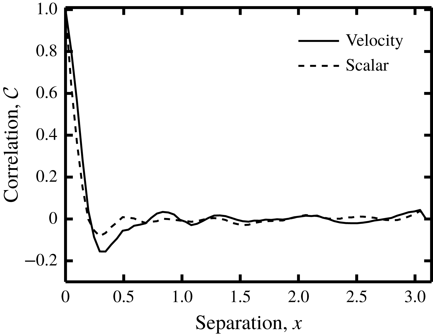
Autocorrelation
 ${\mathcal{C}}$
of the synthetic fluid velocity and scalar fields as functions of the separation distance at
 $t=1$
.

To compare their respective performances we apply both methods to a synthetic scalar field
 $\unicode[STIX]{x1D713}$
in a two-dimensional (2-D) incompressible, decaying turbulent flow on a square, biperiodic domain of size
 $L=2\unicode[STIX]{x03C0}$
. We generate a reference velocity field
 $\boldsymbol{v}$
and a reference scalar field
 $\unicode[STIX]{x1D713}$
using numerical simulation of the hydrodynamic equations and the scalar transport equation in the absence of forcing mechanisms (equation (2.11)). Spatial derivatives in these equations are computed using the Fourier basis functions. Time integration is performed using the second-order explicit Adams–Bashforth scheme for the advection terms and the second-order implicit Crank–Nicolson scheme for the diffusion terms. The number of grid points is
 $N^{2}=128^{2}$
and the numerical integration time step is
 $\unicode[STIX]{x0394}t=1\times 10^{-3}$
. The reconstruction is applied to the time interval
 $0<t<4$
. The initial reference velocity and scalar fields are constructed by assigning random numbers to the Fourier components of the wave vectors with absolute value
 $|\boldsymbol{k}|\leqslant 8$
, while the remaining Fourier components are assumed zero. The initial velocity and scalar fields are normalised, such that
 ${\mathcal{U}}=\Vert \boldsymbol{v}\Vert =1$
and
 $\Vert \unicode[STIX]{x1D713}\Vert =1$
at
 $t=0$
. The diffusivity is
 $\unicode[STIX]{x1D706}=2.2\times 10^{-3}$
and the viscosity is
 $\unicode[STIX]{x1D708}=7.3\times 10^{-4}$
, which corresponds to a Reynolds number of
 $Re={\mathcal{U}}L/\unicode[STIX]{x1D708}=8.6\times 10^{3}$
based on and the initial velocity scale
 ${\mathcal{U}}$
and a Schmidt number of
 $Sc=\unicode[STIX]{x1D708}/\unicode[STIX]{x1D706}=1/3$
, indicating that the smallest velocity length scale is of the same order of magnitude as the smallest scalar length scale.
To quantify the size of the turbulent structures we compute the autocorrelation function
 ${\mathcal{C}}$
, which is plotted for both
 $\boldsymbol{v}$
and
 $\unicode[STIX]{x1D713}$
at
 $t=1$
in figure 1. Defining the correlation length scale
 ${\mathcal{L}}$
as the distance where
 ${\mathcal{C}}=1/2$
, we observe from figure 1 that for both
 $\boldsymbol{v}$
as well as for
 $\unicode[STIX]{x1D713}$
,
 ${\mathcal{L}}\sim 10^{-1}$
at
 $t=1$
. Given the velocity scale of
 ${\mathcal{U}}\approx 1$
we estimate the correlation time as
 ${\mathcal{T}}={\mathcal{L}}/{\mathcal{U}}\sim 10^{-1}$
. It is noted that in decaying turbulence
 ${\mathcal{L}}$
and
 ${\mathcal{T}}$
grow in time (not shown) and the above numbers are order of magnitude estimates. With time, the decaying flow field looses structure, and the spatial and temporal derivatives weaken. Therefore to stringently test both SIV methods, we restrict the reconstruction to
 $0<t<4$
.
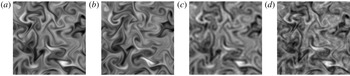
(a,b) Two consecutive samples at
 $t=1$
(a) and
 $t=1.4$
(b) of the synthetic scalar field, using a sampling time of
 $\unicode[STIX]{x1D70F}=0.4$
. (c) Low pass filtered, synthetic scalar field, using a cutoff wavenumber of
 $|\boldsymbol{k}_{c}|L/(2\unicode[STIX]{x03C0})=24$
. (d) Noisy, synthetic scalar field, using a noise level of
 $\unicode[STIX]{x1D702}=0.5$
.
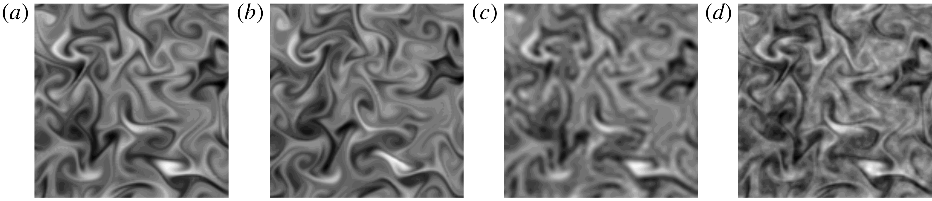
In § 3.2 we study the effect of the temporal resolution on the velocity reconstruction, by using varying sampling times
 $\unicode[STIX]{x1D70F}$
. To illustrate the magnitude of a typical value for
 $\unicode[STIX]{x1D70F}$
, we show in figure 2(a,b) two consecutive scalar field samples, using
 $\unicode[STIX]{x1D70F}=0.4$
.
In § 3.3 we study the effect of the spatial resolution, by subjecting the synthetic scalar field to a low pass filter, with a varying cutoff wavenumber. Figure 2(c) shows a low pass filtered scalar field, where the cutoff wavenumber equals
 $k_{c}=|\boldsymbol{k}_{c}|=48\unicode[STIX]{x03C0}/L$
.
In § 3.4 we study the effect of scalar noise, by adding at each time step an independent random number to each Fourier component of the synthetic scalar field. The random numbers are drawn from a uniform distribution with zero mean and a standard deviation, that is
 $\unicode[STIX]{x1D702}$
times the absolute value of the corresponding Fourier coefficient. Parameter
 $\unicode[STIX]{x1D702}$
is referred to as the noise level. To illustrate the effect of noise, we show in figure 2(d) a synthetic scalar field, that is subjected to a noise level of:
 $\unicode[STIX]{x1D702}\approx 0.5$
(50 %). It is shown in § 3.4, that for very large
 $\unicode[STIX]{x1D702}$
, i.e.
 $\unicode[STIX]{x1D702}\gtrsim 10$
, the finite difference approximations in Method 1 become meaningless, and the reconstruction deteriorates. It is furthermore shown, that for
 $\unicode[STIX]{x1D702}\sim 1$
, which is still a considerable amount of noise, Method 1 may produce accurate results. This behaviour demonstrates the merits of performing the space–time integral minimisation.
3.2 Effect of temporal resolution
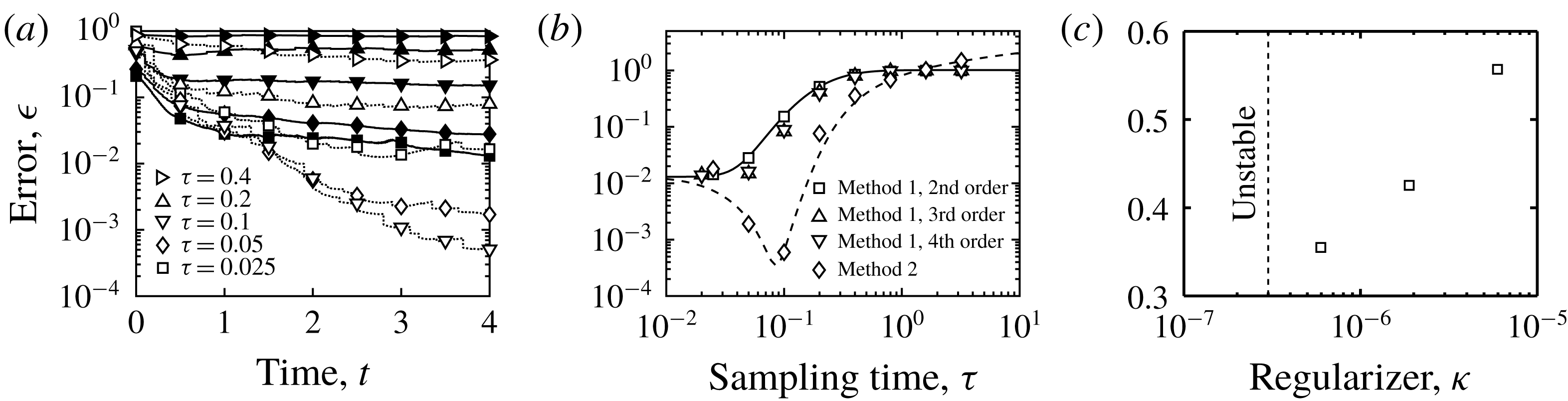
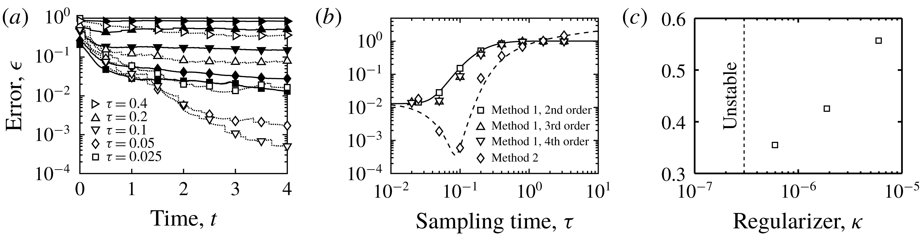
(a) Reconstruction error
 $\unicode[STIX]{x1D716}$
(equation (3.1)) versus time
 $t$
, using noise level
 $\unicode[STIX]{x1D702}=0$
and various sampling times
 $\unicode[STIX]{x1D70F}$
, for Method 1 (filled markers) using regularisation constant
 $\unicode[STIX]{x1D705}=0$
, and for Method 2 (open markers) using
 $\unicode[STIX]{x1D705}=0$
for
 $\unicode[STIX]{x1D70F}<0.1$
and
 $\unicode[STIX]{x1D705}=6\times 10^{-7}$
for
 $\unicode[STIX]{x1D70F}\geqslant 0.1$
. Note, that the correlation time is estimated in § 3.1 as:
 ${\mathcal{T}}\approx 0.1$
. (b)
 $\unicode[STIX]{x1D716}$
versus
 $\unicode[STIX]{x1D70F}$
at
 $t=4$
using
 $\unicode[STIX]{x1D702}=0$
for Method 1 using
 $\unicode[STIX]{x1D705}=0$
, and for Method 2 using
 $\unicode[STIX]{x1D705}=0$
for
 $\unicode[STIX]{x1D70F}<0.1$
and
 $\unicode[STIX]{x1D705}=6\times 10^{-7}$
for
 $\unicode[STIX]{x1D70F}\geqslant 0.1$
. The time derivative of
 $\unicode[STIX]{x1D713}$
in the cost functional of Method 1 (equation (2.1)) is approximated using second-, third- and fourth-order finite difference schemes (equation (2.4)). The lines are drawn to guide the eye. (c)
 $\unicode[STIX]{x1D716}$
versus
 $\unicode[STIX]{x1D705}$
at
 $t=4$
using Method 2,
 $\unicode[STIX]{x1D702}=0$
and
 $\unicode[STIX]{x1D70F}=0.4$
. These data show, that for
 $\unicode[STIX]{x1D70F}=0.4$
, the unregularised Method 2 is unstable, and that the optimum regularisation strength equals
 $\unicode[STIX]{x1D705}\sim 6\times 10^{-7}$
.
We start by studying the accuracy of Method 1 in the absence of noise, i.e.
 $\unicode[STIX]{x1D702}=0$
, as a function of the sampling time
 $\unicode[STIX]{x1D70F}$
, which has been varied between 0.025 and 3.2. Unless stated otherwise we use the second-order finite difference approximation (equation (2.4)) of
 $\unicode[STIX]{x2202}_{t}\unicode[STIX]{x1D713}$
in (2.1). All the corresponding reconstruction runs were stable with zero regularisation strength
 $\unicode[STIX]{x1D705}=0$
. Figure 3(a) shows for various values of
 $\unicode[STIX]{x1D70F}$
the reconstruction error
 $\unicode[STIX]{x1D716}$
as a function of time.
 $$\begin{eqnarray}\unicode[STIX]{x1D716}=\frac{\Vert \boldsymbol{u}-\boldsymbol{v}||^{2}}{\Vert \boldsymbol{v}\Vert ^{2}},\end{eqnarray}$$
where it is recalled, that
 $\boldsymbol{u}$
is the reconstructed velocity and
 $\boldsymbol{v}$
is the reference velocity field. It is noted, that for clarity, figure 3(a) only shows results up to
 $\unicode[STIX]{x1D70F}=0.4$
, since results for larger
 $\unicode[STIX]{x1D70F}$
fall on top of each other. It is seen in figure 3(a), that with time, the error first decreases and after a few time units reaches a steady value. Recalling the time segmentation described in § 2, this time dependent behaviour indicates, that the reconstruction depends on the quality of the initial guess for the initial condition at the start of each segment. In the first segment the initial guess is zero, while in each consecutive segment the initial guess gets closer to the ‘exact’ solution, explaining the observed decrease in
 $\unicode[STIX]{x1D716}$
with time.
Figure 3(b) shows the final and steady error
 $\unicode[STIX]{x1D716}$
, which is taken at
 $t=4$
, as a function of the sampling time, in the range:
 $0.025\leqslant \unicode[STIX]{x1D70F}\leqslant 3.2$
. The reconstruction error
 $\unicode[STIX]{x1D716}$
is seen to increase with
 $\unicode[STIX]{x1D70F}$
. There are two causes for this behaviour. The first cause is related to the ill posedness of the initial value problem for chaotic systems, which corresponds to the cost functional developing multiple minima, when
 $\unicode[STIX]{x1D70F}$
exceeds a threshold (see e.g. Pires, Vautard & Talagrand Reference Pires, Vautard and Talagrand1996). Figure 3(b) shows that in the present system this threshold is of the order of 0.1, which is in the same range as the estimated correlation time
 ${\mathcal{T}}$
; see § 3.1. The second cause for the increase in
 $\unicode[STIX]{x1D716}$
with
 $\unicode[STIX]{x1D70F}$
(figure 3
b) is the error in the discretisation of
 $\unicode[STIX]{x2202}_{t}\unicode[STIX]{x1D713}$
in (2.1). To study this effect we have repeated the reconstruction, using third- and fourth-order finite difference schemes (equation (2.4)). The results in figure 3(b) show only marginal improvements, by using higher-order time discretisation schemes. Therefore we use the second-order scheme in the remainder of this work.
Next, we evaluate the performance of Method 2 in reconstructing the velocity field from noise-free scalar fields (
 $\unicode[STIX]{x1D702}=0$
). We still focus on the effect of the sampling time
 $\unicode[STIX]{x1D70F}$
, which is varied between 0.025 and 3.2. We found that in the current set-up, Method 2 is unstable for
 $\unicode[STIX]{x1D70F}\gtrsim 0.1$
. Since we employ the ‘direct numerical simulation’ technique, this instability is not triggered by a lack of energy dissipation due to unresolved scales. Instead, it is believed, that the instability is related to the ill posedness of the problem, as discussed above. In order to stabilise these cases we use regularisation
 $\unicode[STIX]{x1D705}$
-terms in (2.10). The optimal
 $\unicode[STIX]{x1D705}$
is determined by trial and error. Figure 3(c) shows the reconstruction error
 $\unicode[STIX]{x1D716}$
(equation (3.1)) for various values of the regularisation strength
 $\unicode[STIX]{x1D705}$
using
 $\unicode[STIX]{x1D70F}=0.4$
. It is seen, that the optimum value is
 $\unicode[STIX]{x1D705}\sim 6\times 10^{-7}$
, while for smaller values the method is unstable, and for larger values the error increases.
Figure 3(a,b) shows the reconstruction error
 $\unicode[STIX]{x1D716}$
of Method 2, alongside with that of Method 1. Figure 3(a) shows
 $\unicode[STIX]{x1D716}$
as a function of time
 $t$
for various values of the sampling time
 $\unicode[STIX]{x1D70F}$
, while figure 3(b) shows
 $\unicode[STIX]{x1D716}$
as a function of
 $\unicode[STIX]{x1D70F}$
for a fixed value of
 $t=4$
. For Method 2 we have used
 $\unicode[STIX]{x1D705}=0$
for
 $\unicode[STIX]{x1D70F}<0.1$
and
 $\unicode[STIX]{x1D705}=6\times 10^{-7}$
for
 $\unicode[STIX]{x1D70F}\geqslant 0.1$
. The comparison demonstrates the improved performance of Method 2 in the range
 $0.05<\unicode[STIX]{x1D70F}<1$
. It is moreover observed, that with increasing
 $\unicode[STIX]{x1D70F}$
, the error of Method 2 continues to grow, and the corresponding reconstructed velocity becomes increasingly noisy and finally unstable. This behaviour is in contrast to that of Method 1, whose error saturates, and whose solution remains stable for large
 $\unicode[STIX]{x1D70F}$
. We elaborate on the stability issue in § 3.4. It is noted, that for
 $\unicode[STIX]{x1D70F}\gtrsim 1$
, the error of Method 1:
 $\unicode[STIX]{x1D716}\sim 1$
, which is smaller than
 $\unicode[STIX]{x1D716}\gtrsim 1$
for Method 2, but both reconstructions are too inaccurate to be useful.
3.3 Effect of spatial resolution
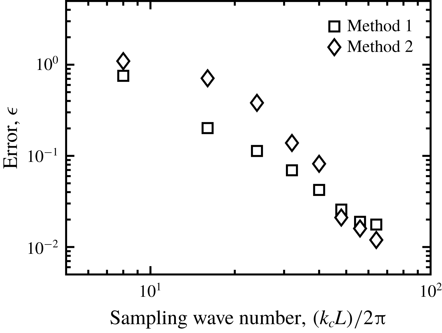
Reconstruction error
 $\unicode[STIX]{x1D716}$
(equation (3.1)) versus low pass, cutoff wavenumber
 $k_{c}$
, using sampling time
 $\unicode[STIX]{x1D70F}=0.025$
, noise level
 $\unicode[STIX]{x1D702}=0$
and regularisation strength
 $\unicode[STIX]{x1D705}=0$
, for Method 1 and Method 2.

Next we consider the effect of the spatial measurement resolution, on the performance of Method 1 and Method 2. Since our numerical method operates in Fourier space, we vary the spatial resolution, by subjecting the synthetic scalar fields, to a low pass filter, with a variable cutoff wavenumber
 $k_{c}=|\boldsymbol{k}_{c}|$
. In physical space, this operation is equivalent to coarse graining, with a grain size of
 ${\sim}k_{c}^{-1}$
. Since the unfiltered reference field has a spatial resolution of
 $128\times 128$
, and the domain size is
 $L=2\unicode[STIX]{x03C0}$
, the maximum cutoff wavenumber is 64, which corresponds to no filtering. In the following, we use Method 1 and Method 2 to reconstruct the velocity field on the
 $128\times 128$
grid, based on low pass filtered scalar fields, where
 $k_{c}$
is varied between 8 and 64. We use a sampling time of
 $\unicode[STIX]{x1D70F}=0.025$
, a noise level of
 $\unicode[STIX]{x1D702}=0$
and a regularisation strength of
 $\unicode[STIX]{x1D705}=0$
. Under these conditions, both methods provide equal accuracy, with
 $\unicode[STIX]{x1D716}\approx 10^{-2}$
, when applied to the fully resolved (
 $k_{c}=64$
) synthetic scalar field; see figure 3(b).
In figure 4, we compare the reconstruction error of both methods, as a function of the spatial resolution of the measured scalar field, i.e. as a function of
 $k_{c}$
. As expected the error of both methods increases with decreasing
 $k_{c}$
, i.e. when removing flow features with increasing length scales. Perhaps unexpected, at low spatial resolution, Method 2 somewhat underperforms compared to Method 1. This result reflects that both methods are based on the same governing equations, and therefore they reconstruct the missing information in a similar fashion. It furthermore shows, that the Fourier approximation of the derivatives of resolved modes, is unaffected by the removal of unresolved modes. When the (resolved) modes are contaminated by noise however, then the discretisation errors do become important, and this is discussed in § 3.4.
3.4 Effect of noise
Vorticity visualisation at
 $t=4$
of the reference simulation (a) and of the reconstruction using
 $\unicode[STIX]{x1D70F}=0.1$
and
 $\unicode[STIX]{x1D702}=0.29$
for Method 1 using
 $\unicode[STIX]{x1D705}=0$
(b),
 $\unicode[STIX]{x1D705}=1.9\times 10^{-4}$
(c),
 $\unicode[STIX]{x1D705}=6.0\times 10^{-3}$
(d), and for Method 2 using
 $\unicode[STIX]{x1D705}=6.0\times 10^{-7}$
(e).

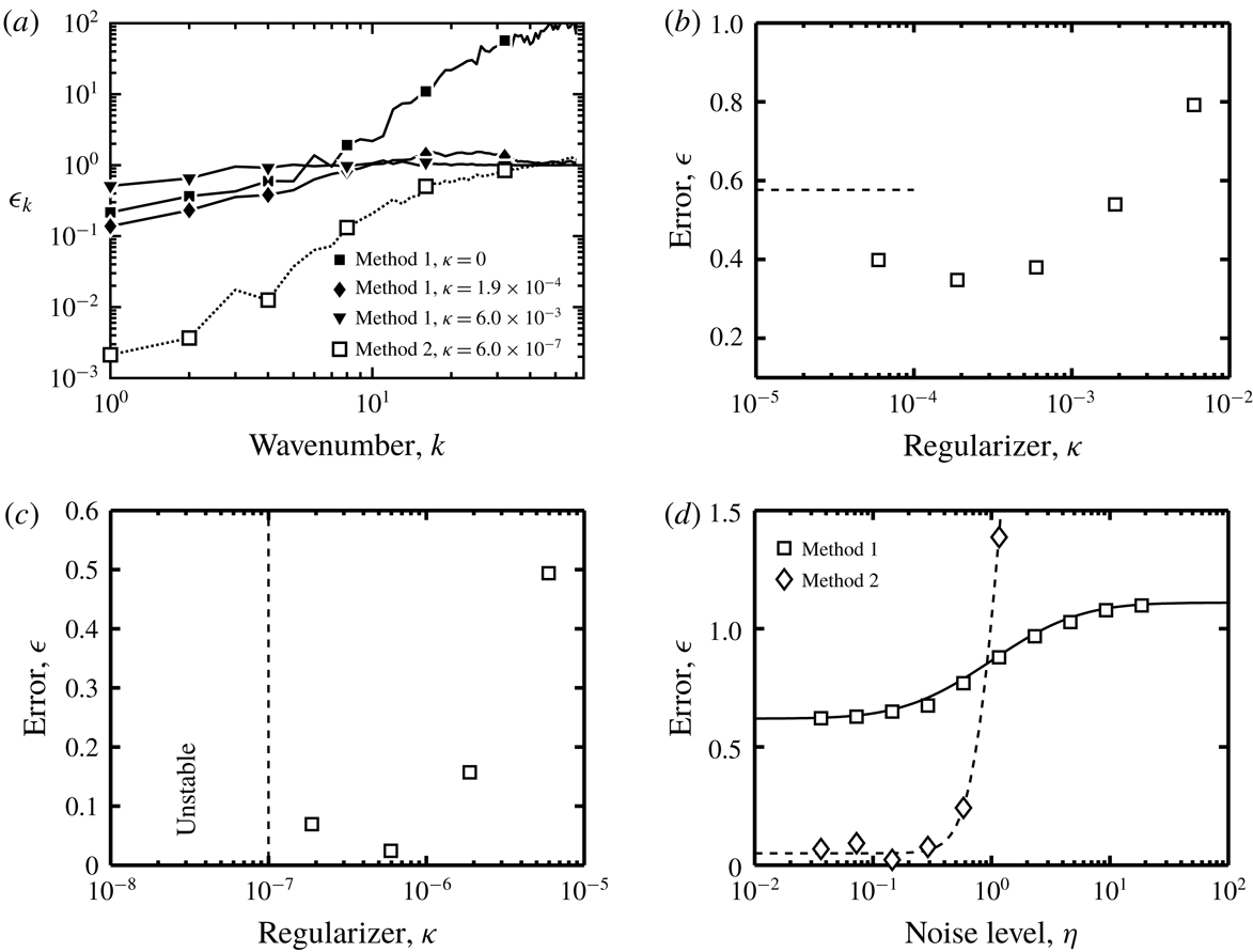
We now turn our focus to the effect of the scalar noise. Figure 5(b) visualises the vorticity of the reconstructed flow field
 $\unicode[STIX]{x1D735}\times \boldsymbol{u}$
using Method 1,
 $\unicode[STIX]{x1D70F}=0.1$
,
 $\unicode[STIX]{x1D702}=0.29$
and
 $\unicode[STIX]{x1D705}=0$
. For comparison we show the reference solution in figure 5(a). It is noted that the vorticity fields in figure 5 vary in magnitude and to allow a proper visualisation we have used different mappings between the vorticity and the grey scale values in each of the panels.
As expected figure 5(b) shows, that scalar noise results in velocity reconstruction noise. For the case of figure 5(b) the noise is concentrated at the small length scales. As an effect the large-scale flow structures, which are reasonably accurately reconstructed, are hardly visible in figure 5(b). To substantiate this point we plot in figure 6(a) the relative error spectrum
 $\unicode[STIX]{x1D716}_{k}$
:
 $$\begin{eqnarray}\unicode[STIX]{x1D716}_{k}=\frac{\displaystyle \left|\int \left[\boldsymbol{u}-\boldsymbol{v}\right]\exp (-\text{i}\boldsymbol{k}\boldsymbol{\cdot }\boldsymbol{x})\,\text{d}V\right|^{2}}{\displaystyle \left|\int \boldsymbol{v}\exp (-\text{i}\boldsymbol{k}\boldsymbol{\cdot }\boldsymbol{x})\,\text{d}V\right|^{2}}.\end{eqnarray}$$
This quantity measures the relative difference between the reconstruction and the reference velocity field, at wave vectors with an absolute value of
 $k$
. The filled squares in figure 6(a) correspond to the case, that is visualised in figure 5(b). It is seen that the large scales are captured relatively well with:
 $\unicode[STIX]{x1D716}_{k}\sim 10^{-1}$
. The small scales on the other hand are heavily contaminated by noise with:
 $\unicode[STIX]{x1D716}_{k}\sim 10^{2}$
.
In order to suppress the large wavenumber noise in the reconstruction, a regularisation term is added to the cost functional (equation (2.1)). The value for the regularisation constant
 $\unicode[STIX]{x1D705}$
must be chosen with care as to suppress the small-scale noise, while leaving the large-scale flow structures intact. Figure 5(c,d) shows that with increasing
 $\unicode[STIX]{x1D705}$
, the small-scale noise diminishes but also the large-scale structures become less accurate. This is confirmed by the relative error spectra in figure 6(a), which shows that for intermediate
 $\unicode[STIX]{x1D705}=1.9\times 10^{-4}$
(filled diamonds) the error is reduced over the entire spectrum. For large
 $\unicode[STIX]{x1D705}=6.0\times 10^{-3}$
(filled triangles) on the other hand, although slightly better at the small scales, the error increases significantly at the large scales.
(a) Relative error spectrum
 $\unicode[STIX]{x1D716}_{k}$
(equation (3.2)) versus wavenumber
 $k$
using sampling time
 $\unicode[STIX]{x1D70F}=0.1$
and noise level
 $\unicode[STIX]{x1D702}=0.29$
for Method 1 (filled markers) using various regularisation constants
 $\unicode[STIX]{x1D705}$
, and for Method 2 (open markers) using
 $\unicode[STIX]{x1D705}=6.0\times 10^{-7}$
. (b) Reconstruction error
 $\unicode[STIX]{x1D716}$
(equation (3.1)) versus
 $\unicode[STIX]{x1D705}$
using Method 1,
 $\unicode[STIX]{x1D70F}=0.1$
and
 $\unicode[STIX]{x1D702}=0.29$
. The dashed line indicates the
 $\unicode[STIX]{x1D716}$
-value for
 $\unicode[STIX]{x1D705}=0$
. (c)
 $\unicode[STIX]{x1D716}$
versus
 $\unicode[STIX]{x1D705}$
using Method 2,
 $\unicode[STIX]{x1D70F}=0.1$
and
 $\unicode[STIX]{x1D702}=0.29$
. (d)
 $\unicode[STIX]{x1D716}$
versus
 $\unicode[STIX]{x1D702}$
using
 $\unicode[STIX]{x1D70F}=0.2$
. Comparison between Method 1 using
 $\unicode[STIX]{x1D705}=6.0\times 10^{-4}$
and Method 2 using
 $\unicode[STIX]{x1D705}=6.0\times 10^{-7}$
.

Figure 6(b) shows the corresponding reconstruction error
 $\unicode[STIX]{x1D716}$
(equation (3.1)) as a function of
 $\unicode[STIX]{x1D705}$
. The figure demonstrates that for
 $\unicode[STIX]{x1D705}\sim 6\times 10^{-4}$
the reconstruction error is minimum. For this optimum regularisation strength there is however still small-scale noise observed in the visualisation (figure 5
c). Despite this the large-scale structures are distinguishable and resemble those of the reference field (figure 5
a). Increasing
 $\unicode[STIX]{x1D705}$
beyond the optimum value results in a smooth velocity reconstruction, but also in a large
 $\unicode[STIX]{x1D716}$
. The corresponding large-scale structures (figure 5
d) no longer resemble the reference field (figure 5
a). It is noted that for severe noise levels, up to
 $\unicode[STIX]{x1D702}=16$
, Method 1 produced stable results, without regularisation, i.e.
 $\unicode[STIX]{x1D705}=0$
.
The stability behaviour is different for Method 2, where instability is triggered by a relatively small amount of noise
 $\unicode[STIX]{x1D702}\gtrsim 0.1$
. Method 2 can efficiently be stabilised however using the regularisation terms in (2.10). Again the regularisation constant
 $\unicode[STIX]{x1D705}$
was found by trial and error. Figure 6(c) shows the corresponding
 $\unicode[STIX]{x1D716}$
as a function of
 $\unicode[STIX]{x1D705}$
using
 $\unicode[STIX]{x1D70F}=0.1$
and
 $\unicode[STIX]{x1D702}=0.29$
. It is observed that under these conditions, Method 2 is unstable for
 $\unicode[STIX]{x1D705}\lesssim 10^{-7}$
, while for
 $\unicode[STIX]{x1D705}\gtrsim 10^{-7}$
the error is a non-monotonic function of
 $\unicode[STIX]{x1D705}$
with an optimum value at around
 $\unicode[STIX]{x1D705}\sim 6\times 10^{-7}$
. It is noteworthy that this value is roughly the same as in § 3.2, where the instability set in due to a relatively large sampling time
 $\unicode[STIX]{x1D70F}$
. The corresponding vorticity visualisation (figure 5
e) is free of noise and resembles the reference field (figure 5
a) well.
The relative error spectrum
 $\unicode[STIX]{x1D716}_{k}$
in figure 6(a) shows the improved accuracy of Method 2 over Method 1, when confronted with measurement noise, and when using the optimum regularisation parameters. In this regard, it is noted that, as defined in (3.2),
 $\unicode[STIX]{x1D716}_{k}$
clearly visualises the
 $k$
-dependence of the reconstruction error, which is hidden when directly comparing the energy spectra
 $E_{k}$
(not shown):
 $$\begin{eqnarray}E_{k}=\left|\int \boldsymbol{v}\exp (-\text{i}\boldsymbol{k}\boldsymbol{\cdot }\boldsymbol{x})\,\text{d}V\right|^{2}.\end{eqnarray}$$
It may seem peculiar, that the optimum
 $\unicode[STIX]{x1D705}$
for Method 1 (figure 6
b) is three orders of magnitude larger than that for Method 2 (figure 6
c). This difference can be explained however by an order of magnitude analysis of the various terms in the cost functionals for Method 1 (equation (2.1)) and for Method 2 (equation (2.10)). As discussed in § 2 the regularisation terms
 $\unicode[STIX]{x1D705}\Vert \unicode[STIX]{x1D6FB}^{2}\boldsymbol{u}\Vert ^{2}$
and
 $\unicode[STIX]{x1D705}\Vert \unicode[STIX]{x1D6FB}^{2}\unicode[STIX]{x1D719}\Vert ^{2}$
are of the same order of magnitude provided that variables are properly scaled and the Schmidt number is
 $Sc=\unicode[STIX]{x1D708}/\unicode[STIX]{x1D706}\sim 1$
. To estimate the appropriate value for
 $\unicode[STIX]{x1D705}$
we balance the magnitude of the regularisation terms to that of the remaining term, which is
 $\Vert \unicode[STIX]{x2202}_{t}\unicode[STIX]{x1D713}+\unicode[STIX]{x1D735}\boldsymbol{\cdot }(\boldsymbol{u}\unicode[STIX]{x1D713})-\unicode[STIX]{x1D706}\unicode[STIX]{x1D6FB}^{2}\unicode[STIX]{x1D713}\Vert ^{2}$
in Method 1 and
 $\Vert \unicode[STIX]{x1D719}-\unicode[STIX]{x1D713}\Vert ^{2}$
in Method 2. The ratio of
 $\unicode[STIX]{x1D705}$
in Method 1:
 $\unicode[STIX]{x1D705}_{1}$
to that of Method 2:
 $\unicode[STIX]{x1D705}_{2}$
is therefore proportional to the ratio of these remaining terms, i.e.
 $\unicode[STIX]{x1D705}_{1}/\unicode[STIX]{x1D705}_{2}\sim \Vert \unicode[STIX]{x2202}_{t}\unicode[STIX]{x1D713}+\unicode[STIX]{x1D735}\boldsymbol{\cdot }(\boldsymbol{u}\unicode[STIX]{x1D713})-\unicode[STIX]{x1D706}\unicode[STIX]{x1D6FB}^{2}\unicode[STIX]{x1D713}\Vert ^{2}/\Vert \unicode[STIX]{x1D719}-\unicode[STIX]{x1D713}\Vert ^{2}$
. Assuming that
 $\boldsymbol{u}\sim \unicode[STIX]{x1D713}\sim \unicode[STIX]{x1D719}\sim 1$
and that
 $\unicode[STIX]{x1D735}\sim k_{max}=N/2$
we estimate
 $\unicode[STIX]{x1D705}_{1}/\unicode[STIX]{x1D705}_{2}\sim (N/2)^{2}\approx 4\times 10^{3}$
, where
 $N=128$
is the number of grid points per dimension. This explains that Method 1 requires a regularisation strength that is three orders of magnitude larger than that of Method 2.
In figure 6(d) we compare the reconstruction error
 $\unicode[STIX]{x1D716}$
for Method 1 and Method 2 as a function of the noise level
 $\unicode[STIX]{x1D702}$
, that has been varied between
 $3.1\times 10^{-2}\leqslant \unicode[STIX]{x1D702}\leqslant 1.6\times 10^{1}$
. Here we use a sampling time of
 $\unicode[STIX]{x1D70F}=0.2$
and we have kept the regularisation constant fixed to
 $\unicode[STIX]{x1D705}=6\times 10^{-4}$
for Method 1 and to
 $\unicode[STIX]{x1D705}=6\times 10^{-7}$
for Method 2. It is noted that these
 $\unicode[STIX]{x1D705}$
values were optimised for
 $\unicode[STIX]{x1D70F}=0.1$
and
 $\unicode[STIX]{x1D702}=0.29$
(see figure 6
b,c), which are different from the parameters used in figure 6(d). It would be possible to derive optimum
 $\unicode[STIX]{x1D705}$
values for each data point in figure 6(d), but this would only marginally alter the results and has therefore been omitted. Figure 6(d) shows that for
 $\unicode[STIX]{x1D702}\lesssim 0.1$
the error in both methods is insensitive to
 $\unicode[STIX]{x1D702}$
. For
 $\unicode[STIX]{x1D702}\gtrsim 0.1$
the error in Method 1 grows gradually and reaches a stable value for
 $\unicode[STIX]{x1D702}\gtrsim 10$
. The error in Method 2, on the other hand, grows rapidly for
 $\unicode[STIX]{x1D702}\gtrsim 0.1$
, and for this particular
 $\unicode[STIX]{x1D705}$
the solution becomes unstable for
 $\unicode[STIX]{x1D702}\gtrsim 1$
. Although Method 1 is stable for large noise levels
 $\unicode[STIX]{x1D702}\gtrsim 10$
, the reconstruction error of Method 1 equals:
 $\unicode[STIX]{x1D716}\sim 1$
, under these conditions.
4 Application to soap film turbulence
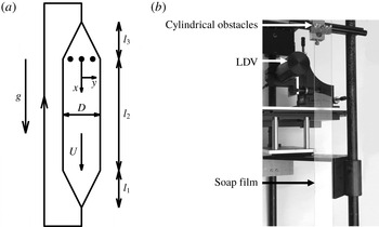
(a) Gravity
 $g$
drives a
 $3~\unicode[STIX]{x03BC}\text{m}$
thick soap film with a velocity of around
 $U=2~\text{m}~\text{s}^{-1}$
between two wires, that form a vertical channel, with a diverging width, a constant width
 $D=0.06$
m and a converging width. The lengths of the respective sections are
 $l_{3}=0.7$
m,
 $l_{2}=1$
m and
 $l_{1}=0.45$
m. Soap is collected at the channel exit, pumped upwards and injected at the channel entrance. Three cylinders are placed in the film to generate 2-D turbulence. The downstream distance to the cylinders and the wall normal distance to the channel centreline are denoted
 $x$
and
 $y$
, respectively. (b) Photograph of the set-up, showing the cylindrical obstacles, the LDV probe and the soap film.

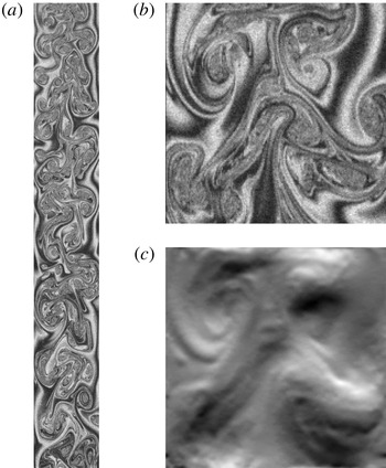
(a) The soap film thickness field between
 $0.06<x<0.43$
m and
 $-0.027<y<0.027$
m is visualised by the interference pattern of reflected light. (b) The interference pattern in an interrogation window between
 $0.201<x<0.254$
m and
 $-0.027<y<0.027$
m. (c) The
 $y$
component of the reconstructed velocity field in the interrogation window, that corresponds to the interference pattern, shown in figure 8(b).

Finally, we apply SIV to experimental data of the thickness field of a turbulent soap film. The experimental set-up is sketched in figure 7(a) and a photograph of the set-up is provided in figure 7(b). This set-up has previously been used to study two dimensional turbulence; see e.g. Greffier, Amarouchene & Kellay (Reference Greffier, Amarouchene and Kellay2002). In the experiment, a 2 % detergent (Fairy Dreft) in water solution is injected at the top of a two-dimensional channel, that consists of two nylon wires, with a thickness of 0.5 mm. The channel has a straight section with a length of
 $l_{2}=1$
m and a width of
 $D=0.06$
m. The wires are configured to form a diverging channel entrance and a converging channel exit, as to allow fluid injection and collection, respectively. As sketched in figure 7(a), three cylinders with a radius of 4 mm are placed in the film. The distance between the cylinder centres is 12 mm. The cylinders induce flow disturbances that evolve into 2-D turbulence; see figure 8(a). The downstream distance to the cylinders is denoted
 $x$
and the distance to the centreline is denoted
 $y$
. Film thickness and velocity measurements are taken between
 $x=0.06$
and 0.45 m. In this region the flow speed is relatively constant and around
 $U\approx 2~\text{m}~\text{s}^{-1}$
. The average film thickness is estimated as
 $h_{0}=Q/DU=3~\unicode[STIX]{x03BC}\text{m}$
, where the volumetric flow rate is
 $Q=3\times 10^{-7}~\text{m}^{3}~\text{s}^{-1}$
.
Velocity fluctuations induce fluctuations in the film thickness
 $h(x,y,t)$
. Experiments under similar conditions have shown, that these fluctuations are around
 $h_{rms}\approx 100$
nm (Greffier et al.
Reference Greffier, Amarouchene and Kellay2002), which are small compared to the average thickness of
 $h_{0}\approx 3~\unicode[STIX]{x03BC}\text{m}$
. It has been argued theoretically (Bruinsma Reference Bruinsma1995), as well as experimentally (Wu et al.
Reference Wu, Martin, Kellay and Goldburg1995; Greffier et al.
Reference Greffier, Amarouchene and Kellay2002), that the film behaves nearly as a 2-D incompressible fluid, and that the thickness field is a passive scalar, that is being advected by the flow, but with an unusual dissipative term:
 $$\begin{eqnarray}\unicode[STIX]{x2202}_{t}h+\boldsymbol{u}\boldsymbol{\cdot }\unicode[STIX]{x1D735}h=-\unicode[STIX]{x1D70E}\unicode[STIX]{x1D6FB}^{4}h.\end{eqnarray}$$
Here
 $\unicode[STIX]{x1D70E}$
is referred to as the thickness hyper diffusivity, which is conceived to be a function of the fluid viscosity and the fluid surface tension (Bruinsma Reference Bruinsma1995), and has an estimated value of
 $\unicode[STIX]{x1D70E}\sim 10^{-18}~\text{m}^{4}~\text{s}^{-1}$
.
In the experiment, variations in
 $h$
are visualised by illuminating the film with eight mercury lamps (Proxistar 85w 5500k) behind a diffuser and recording the reflected light using a high speed colour camera (Phantom v641), with an exposure time of 300
 $\unicode[STIX]{x03BC}\text{s}$
, and a frame rate of 2000 Hz. Reflections from both sides of the film produce an interference pattern in the recorded image
 $\unicode[STIX]{x1D713}(x,y,t)$
, as shown in figure 8(a,b). The pattern is sharpened by isolating the green channel from the recordings. The interference pattern is periodic, when
 $h$
varies over half of the wavelength of the recorded light. However, since variations in
 $h$
are fewfold smaller than the wavelength, this periodicity may be ignored. Therefore,
 $\unicode[STIX]{x1D713}$
is assumed to be proportional to
 $h$
, and to behave as a passive scalar.
Since the exact form of (4.1) is uncertain (Chomaz Reference Chomaz2001; Auliel et al.
Reference Auliel, Castro, Sosa and Artana2015), and since Method 2 requires diffusive regularisation (
 $\unicode[STIX]{x1D705}$
-terms in (2.10)), we do not attempt to accurately reconstruct the dissipative range of the scalar energy spectrum. As an effect, we do not incorporate the fourth-order diffusion of (4.1) into Method 2, but instead, we replace
 $-\unicode[STIX]{x1D70E}\unicode[STIX]{x1D6FB}^{4}h$
in (4.1), with the usual, second-order diffusion
 $\unicode[STIX]{x1D706}\unicode[STIX]{x1D6FB}^{2}h$
, and apply Method 2 without further modification. The substitute diffusivity (
 $\unicode[STIX]{x1D706}$
in (2.11)) is chosen to be equal to the kinematic viscosity, which is assumed to be that of water
 $\unicode[STIX]{x1D706}=\unicode[STIX]{x1D708}=10^{-6}~\text{m}^{2}~\text{s}^{-1}$
. Furthermore, to stabilise the method, we use a regularisation strength of
 $\unicode[STIX]{x1D705}=1.2\times 10^{-11}~\text{m}^{4}$
. Despite these unphysical assumptions at the dissipative scales, it is shown below, that Method 2 correctly reproduces the statistics of the energy containing velocity fluctuations.
It is noted, that for this case, Method 1 (equation (2.1)) does not produce a reasonable velocity reconstruction (not shown). This is most likely due to inaccurate approximations of the spatial derivatives of the noisy, high frequency content of the interference patterns (figure 8 b). To improve on these aspects, we have developed Method 2, which does not rely on computing spatial nor temporal derivatives of the measured scalar field. Therefore, the subsequent discussion focusses on Method 2.
We apply Method 2 to a square domain (interrogation window) with a size of
 $0.053$
m. A snapshot of the recorded light intensity
 $\unicode[STIX]{x1D713}$
in the window is shown in figure 8(b). The velocity and the scalar fields are reconstructed on a computational grid, where the number of grid points
 $N^{2}=180^{2}$
is one quarter of the number of pixels in the interrogation window, which corresponds to a grid spacing of
 $\unicode[STIX]{x0394}x=2.94\times 10^{-4}$
m. The computational time step is
 $\unicode[STIX]{x0394}t=2\times 10^{-5}$
s, which is one twenty-fifth of the sampling time
 $\unicode[STIX]{x1D70F}=5\times 10^{-4}$
s.
Method 2 assumes periodic boundary conditions, which are not satisfied experimentally. In order to mitigate the detrimental effects of these unphysical conditions, the interrogation window moves downwards with a velocity of
 $1.88~\text{m}~\text{s}^{-1}$
. In the moving window the turbulent eddies evolve without being advected by the mean flow, and can therefore be observed for a long period of time. Furthermore, the moving window minimises the influx of unknown information at the cross-stream boundaries.
Figure 8(c) shows a snapshot of the
 $y$
-component of the velocity reconstruction. It is seen that effects, due to the assumed periodicity of the experimental data, are confined to a thin (few pixels) region at the cross-stream boundaries. Apparently these effects propagate from the boundaries inward with a speed, that is small compared to the speed of the reconstruction.
The total recorded time is one second, which corresponds to 2000 frames. The interrogation window takes 0.17 s to move from the top to the bottom of the recorded image. This translation corresponds to a sequence of 340 images. From the 2000 recorded images, we extract a total of 30 such sequences, by varying the time, at which the window starts moving from the top to the bottom. This starting time is increased by 0.028 s, for each consecutive sequence, which corresponds to the translation of the window over its own size.
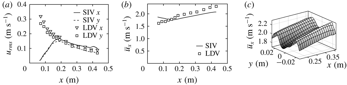
(a) The standard deviation of the velocity components
 $u_{x,rms}$
and
 $u_{y,rms}$
for
 $y=0$
as functions of
 $x$
. Comparison between SIV reconstruction (lines) and LDV measurement (markers). (b) The mean streamwise velocity component
 $\overline{u}_{x}$
for
 $y=0$
as a function of
 $x$
. Comparison between SIV reconstruction (line) and LDV measurement (markers). (c) The reconstructed, mean streamwise velocity component
 $\overline{u}_{x}$
as a function of
 $x$
and
 $y$
. The cylinders induce a cross-stream variation of
 $\overline{u}_{x}$
with a local minimum on the centreline.

To validate Method 2 we compare the reconstructed velocity statistics to laser Doppler velocimetry (LDV) measurements of the streamwise
 $x$
and wall normal
 $y$
velocity components on the centreline
 $y=0$
as a function of the downstream position
 $x$
. To this end, the fluid is dispersed with 1.1
 $\unicode[STIX]{x03BC}\text{m}$
polystyrene beads (SIGMA). Figure 9(a) shows the measured profiles of the standard deviations, i.e. turbulent intensities, of the streamwise velocity
 $u_{x,rms}$
(triangles) and wall normal velocity
 $u_{y,rms}$
(squares). The data show that
 $u_{y,rms}$
is 5 % smaller than
 $u_{x,rms}$
and both quantities decrease as functions of
 $x$
. In the same figure, we show the reconstructed
 $u_{x,rms}$
(solid line) and
 $u_{y,rms}$
(dashed line). These quantities are zero at the start of the reconstruction, which is at
 $x=0.06$
m, and increase until
 $x=0.2$
m, after which they decrease. The initial growth of the turbulent intensity reflects, that the reconstruction requires time to develop. As discussed in § 3.2, this development is related to the time segmentation, where the initial guess for the reconstruction of each segment is taken from the reconstruction of the previous segment. Therefore the reconstructed turbulent intensity is zero at
 $x=0.06$
m, increases with
 $x$
, and approaches the converged profile at
 $x=0.2$
m. For
 $x>0.2$
m the reconstructed
 $u_{y,rms}$
is 5 % smaller than
 $u_{x,rms}$
, and the profiles are within 5 % of the experimental data.
In figure 9(b) we show the profile of the mean streamwise velocity component
 $\overline{u}_{x}$
, obtained by LDV (squares). It is observed, that the mean flow accelerates from
 $\overline{u}_{x}=1.6~\text{m}~\text{s}^{-1}$
at
 $x=0.06$
m to
 $\overline{u}_{x}=2.4~\text{m}~\text{s}^{-1}$
at
 $x=0.43$
m. The corresponding, reconstructed velocity profile is also plotted (line) in figure 9(b). Since the interrogation window moves with a velocity of
 $1.88~\text{m}~\text{s}^{-1}$
, the reconstructed mean flow starts at
 $\overline{u}_{x}=1.88~\text{m}~\text{s}^{-1}$
at
 $x=0.06$
m. With increasing
 $x$
, the reconstructed
 $\overline{u}_{x}$
decreases and approaches the converged profile at
 $x=0.15$
m. After
 $x=0.15$
m, the reconstructed
 $\overline{u}_{x}$
follows the upward trend of the LDV data. There is a 10 % discrepancy between the reconstructed
 $\overline{u}_{x}$
and the LDV data. This may be attributed to steep variations of the mean flow in the
 $y$
-direction (see figure 9
c), in combination with non-converged Reynolds averages, slight off-centreline positioning of the LDV probe, as well as small differences in the positioning of the cylinders, and the flow speed during the video imaging and the LDV data acquisition.
5 Conclusions
We have analysed the performance of two scalar image velocimetry (SIV) methods, being an earlier proposed method (Method 1) and a new method (Method 2). Method 1 requires approximating the space and time derivatives of the measured scalar field
 $\unicode[STIX]{x1D713}$
. Consequently when the scalar measurement resolution is relatively low, or when the scalar fields are relatively noisy, discretisation errors deteriorate the velocity reconstruction. Method 2 improves on these aspect by reconstructing not only the velocity field but also the scalar field, without approximating the space and time derivatives of
 $\unicode[STIX]{x1D713}$
.
We have demonstrated the improvement of Method 2 over Method 1 for a synthetic, 2-D decaying turbulent flow field. The results show that Method 2 produces smaller reconstruction errors, especially when sampling rates are relatively low, and when there is considerable noise in the measurements. Despite being more accurate Method 2 is observed to be less stable than Method 1. Stability is however efficiently restored by adding regularisation terms to the cost functional, which effectively add pulses of hyper viscosity and hyper diffusivity to the conservation equations of momentum and scalar. Although Method 1 is stable without regularisation, a similar regularisation term is shown to improve the accuracy of Method 1, when confronted with noisy measurement data.
To further demonstrate Method 2, we analysed thickness field measurements in a gravity driven, turbulent soap film. The mean and standard deviations of the reconstructed velocity field are within 10 % of laser Doppler velocimetry measurements. The method therefore provides an alternative to particle image velocimetry, to experimentally obtain instantaneous velocity fields in turbulent soap films.
It is finally noted, that, even though we have focussed on 2-D test problems, the proposed Method 2 generalises to three spatial dimensions in a straightforward way. In fact, benefits of Method 2 over Method 1, are expected to be more pronounced in three than in two dimensions. This expectation is based on the notion that Method 2 requires smaller sampling rates than Method 1, and that volumetric sampling rates tend to be smaller than planar sampling rates. For instance acquiring 3-D laser induced fluorescence data requires time consuming sweeps of the laser sheet through the measurement volume (see e.g. Su & Dahm Reference Su and Dahm1996) or 3-D tomographic imaging, which typically operates at a lower sampling rate than planar imaging.
Acknowledgements
This research is supported by the National Research Foundation Singapore under its Campus for Research Excellence and Technological Enterprise programme. The Center for Environmental Sensing and Modeling is an interdisciplinary research group of the Singapore MIT Alliance for Research and Technology. We also wish to acknowledge the financial support from the Department of Mathematics of University College London.