1 Introduction
Reinforcement Learning (RL) (Sutton & Barto, Reference Sutton and Barto1998) has had many successes solving complex, real-world problems. However, unlike supervised machine learning, there is no standard framework for non-experts to easily try out different methods (e.g. Weka, Witten et al., Reference Witten, Frank, Hall and Pal2016), which may pose a barrier to wider adoption of RL methods. While many frameworks exist, such as RL-Glue (Tanner & White, Reference Tanner and White2009), RLPy (Geramifard et al., Reference Geramifard, Klein, Dann, Dabney and How2013), PyBrain (Schaul et al., Reference Schaul, Bayer, Wierstra, Sun, Felder, Sehnke, Rückstieß and Schmidhuber2010), OpenAI-Gym (Brockman et al., Reference Brockman, Cheung, Pettersson, Schneider, Schulman, Tang and Zaremba2016) and others, they all assume some and sometimes even a substantial amount of RL knowledge. Substantial effort is required to add new tasks or instantiate different techniques within these frameworks. Another barrier to wider adoption of RL methods, which is the focus of this article, is the fact that injecting human knowledge (which can significantly improve the speed of learning) can be difficult for a human designer.
When designing an RL agent, human designers must face the question about how much human knowledge to inject into the system and, more importantly, which approach to use for injecting the desired knowledge. From the AI research perspective, the more an agent can learn autonomously, the more interesting and beneficial the agent will be. From the engineering or more practical perspective, more human input is desirable as it can help improve the agent’s learning as well as the speed at which the agent learns. However, this knowledge is only useful as long as it is practical for it to be gathered and leveraged by the human designer. In order for RL methods to move beyond requiring developers to fully understand the black arts of generalization, approximation and biasing, it is critical that the community better understand if and how both expert and non-expert humans can provide useful information for an RL agent. This article takes the problem to the field and focuses on human designers who have a background in AI and coding, but varying experience in RL.
The baseline approach in this study is to allow no generalization: an agent’s interactions with its environment will immediately affect only its current state in a tabular representation. We will compare this baseline with two widely common speedup approaches: function approximation (FA) (Busoniu et al., Reference Busoniu, Babuska, De Schutter and Ernst2010), and reward shaping (RS) (Mataric, Reference Mataric1994). We further propose and evaluate a novel approach which we name SASS, which stands for State Action Similarity Solutions, which relies on hand-coded state–action similarity functions. We test the three speedup approaches in a first-of-its-kind human study consisting of three experts (highly experienced programmers with an RL background, but not co-authors of this paper) and 48 non-expert computer science studentsFootnote 1 . To that end, three RL tasks of varying complexities are considered:
1. The ‘toy’ task of simple robotic soccer (Littman, Reference Littman1994), providing a basic setting for the evaluation.
2. A large grid-world task named Pursuit (Benda, Reference Benda1985), investigating the three speedup methods on a moderately challenging task.
3. The popular game of Mario (Karakovskiy & Togelius, Reference Karakovskiy and Togelius2012), exemplifying the complexities of instantiating speedup approaches in complex tasks.
Through this human study, we find that the RS technique is the most natural method for most designers, both expert and non-expert, to speed up RL across the three tasks. However, we further find that the newly proposed SASS method can be effectively and efficiently combined with RS, providing an additional speedup in most cases.
This article argues that in order to bring about a wider adoption of RL techniques, specifically of generalization techniques, it is essential to both investigate and develop RL techniques appropriate for both expert and non-expert designers. We hope that this study will encourage other researchers to invest an increased effort in the human factors behind RL and investigate their RL solutions in human studies.
The remainder of the article is organized as follows: in Section 2, we review some preliminaries on RL and survey recent related work. In Section 3, we present the
 $QS$
-learning algorithm that incorporates similarities within the basic
 $Q$
-learning framework and discuss its theoretical foundations. We further propose three notions of state–action similarities and discuss how these similarities can be defined. In Section 4, we present an extensive empirical evaluation of the three tested approaches in three RL tasks. Finally, in Section 5 we provide a summary and list future directions for this line of work.
2 Preliminaries and background
An RL agent generally learns how to interact with an unfamiliar environment (Sutton & Barto, Reference Sutton and Barto1998). We define the RL task using the standard notation of a Markov Decision Process (MDP). An MDP is defined as
 $${\cal S},\,{\cal A},\,{\cal T},\,{\cal R},\,\gamma $$
where:
∙
 $${\cal S}$$
is the state-space;
∙
$${\cal A}$$
is the action-space;∙
$${\cal T}\,\colon\,{\cal S}{\times}{\cal A}{\times}{\cal S}\to\left[ {0,1} \right]$$
defines the transition function, where
$${\cal T}$$
(s, a, s′) is the probability of making a transition from state s to state s′ using action a;∙
$${\cal R}\,\colon\,{\cal S}{\times}{\cal A}{\times}{\cal S}\to{\Bbb R}$$
is the reward function; and∙ γ∈[0, 1] is the discount factor, which represents the significance of future rewards compared to present rewards.


We assume
 $${\cal T}$$
and
 $${\cal R}$$
are initially unknown to the agent. In discrete time tasks, the agent interacts in a sequence of time steps. At each time step, the agent observes its state s∈
 $${\cal S}$$
and is required to select an action a∈
 $${\cal A}$$
. The agent then arrives at a new state s′ according to the unknown
 ${\cal T}$
function and receives a reward r according to the unknown
 ${\cal R}$
function. We define an agent’s experience as a tuple 〈s, a, r, s′〉 where action a is taken in state s, resulting in reward r and a transition to the next state, s′. The agent’s objective is to maximize the accumulated discounted rewards throughout its lifetime. Namely, the agent seeks to find a policy
 $$\pi \,\colon\,{\cal S}\mapsto{\cal A}$$
that maximizes the expected total discounted reward (i.e. expected return) from following it.
Temporal difference RL algorithms such as
 $Q$
-learning (Watkins, Reference Watkins1989) approximate an action-value function
 $Q\,\colon\,{\cal S}{\times}{\cal A}\mapsto{\Bbb R}$
, mapping state–action pairs to the expected real-valued discounted return.
 $QR$
-learning updates the
 $$QRS$$
-value estimation according to the temporal difference update rule
 $$Q(s,\,a){\equals}Q(s,\,a){\plus}\alpha (r{\plus}\gamma \max _{{\hskip 18pta'}} Q(s',\,a'){\minus}Q(s,\,a))$$
where α is the learning rate. If both
 ${\cal S}$
and
 ${\cal A}$
are finite sets, the
 $Q$
function can be easily represented in a table, namely in an
 $$\,\mid\hskip -3pt{\cal S}\hskip -3pt\mid\hskip -2pt{\times}\hskip -3pt\mid\hskip -3pt{\cal A\hskip -3pt\mid}$$
matrix, where each state–action pair is saved along with its discounted return estimation. In this case, the convergence of
 $Q$
-learning has been proven in the past (under standard assumptions). See Sutton and Barto (Reference Sutton and Barto1998) for more details. In this study, we focus on the
 $$Q$$
-learning algorithm with a tabular representation of the
 $Q$
function. This scheme is, perhaps, the most basic and commonly applied in RL tasks and allows us to control for many of the confounding factors in human experiments (e.g. implementation complexity).
RL can often suffer from slow learning speeds. To address this problem, designers infuse human-generated, domain-specific knowledge into the agent’s learning process in different ways, enabling better generalization across small numbers of samples. Another interpretation for this approach is allowing the agent to better understand and predict what a ‘human agent’ would do or conclude in a given setting and leverage this prediction to make better decisions on its own (see Rosenfeld & Kraus, Reference Rosenfeld and Kraus2018).
Perhaps the most prominent method for leveraging human knowledge to speedup RL is FA (Busoniu et al., Reference Busoniu, Babuska, De Schutter and Ernst2010). The FA approach focuses on mitigating the costs associated with maintaining and manipulating the value of every state–action pair, as in the usual tabular representation case. Specifically, using FA, a designer needs to abstract the state–action space in a sophisticated manner such that the (presumed) similar states or state–action pairs will be updated together and dissimilar states or state–action pairs are not. This allows the RL learner to quickly generalize each of its experiences such that the value of more than a single state or state–action pair is updated simultaneously. FA is based on the premise that a human designer can recognize features or patterns in the environment by which one can determine a successful policy. Many successful RL applications have used highly engineered state features to bring about a successful learning performance (e.g. ‘the distance between the simulated robot soccer player with the ball to its closest opponent’ and ‘the minimal angle with the vertex at the simulated robot soccer player with the ball between the closest teammate and any of the opponents’ (Stone et al., Reference Stone, Kuhlmann, Taylor and Liu2006)). With the recent successes of DeepRL (Mnih et al., Reference Mnih, Kavukcuoglu, Silver, Rusu, Veness, Bellemare, Graves, Riedmiller, Fidjeland, Ostrovski, Petersen, Beattie, Sadik, Antonoglou, King, Kumaran, Wierstra, Legg and Hassabis2015), convolutional neural networks were shown to successfully learn features directly from pixel-level representations. However, such features are not necessarily optimal. A significant amount of designer time is necessary to define the deep neural network’s architecture, and a significant amount of data is required to learn the features.
Another popular approach of injecting human knowledge to an RL learner is RS (Mataric, Reference Mataric1994). RS attempts to bias the RL learner’s decision-making by adding additional localized rewards that encourage a behavior consistent with some prior knowledge of the human designer. Specifically, instead of relying solely on the reward function
 ${\cal R}$
, the agent considered an augmented reward signal R(s, a, s′)+F(s, a, s′) where F is the shaping reward function articulated by the human designer. The RS approach is inspired by Skinner’s recognition of the effectiveness of training an animal by reinforcing successive approximations of the desired behavior (Skinner, Reference Skinner1958). While the use of RS may result in undesirable learned behavior in the general case (e.g. Randløv & Alstrøm, Reference Randløv and Alstrøm1998), if RS is applied carefully (e.g. using the Potential-Based Reward Shaping (PBSR) method (Ng et al., Reference Ng, Harada and Russell1999)), one can guarantee that the resulting learned policy is unaltered and, in many cases, produce a significant speedup. Indeed, RS has been utilized by many successful RL applications, significantly speeding up the agent’s learning process (e.g. ‘encouraging simulated robotic soccer players to spread out across the field’ and ‘encouraging a simulated robotic soccer player to tackle the ball on defense’ (Devlin et al., Reference Devlin, Grze´s and Kudenko2011)).
Another related line of research investigates providing direct biasing from non-expert humans, such as incorporating human-provided feedback (Knox & Stone, Reference Knox and Stone2010; Peng et al., Reference Peng, MacGlashan, Loftin, Littman, Roberts and Taylor2016) or demonstrations (Brys et al., Reference Brys, Harutyunyan, Suay, Chernova, Taylor and Nowé2015). For example, one may ask a non-expert user to teleoperate the agent or provide online feedback for the agent’s actions. These methods do not require significant technical abilities on the part of the human (e.g. programming is not needed). In this article, we consider a possibly complementary approach, leveraging technically able human designers’ knowledge and technical abilities, either in terms of providing an abstraction, a RS function or a similarity function, to improve the agent’s performance. The investigated approaches can be integrated with direct biasing as well. We leave the examination of non-technical methods (e.g. direct biasing) and non-technical designers (e.g. designers who cannot program) for future work.
While the above (and other) methods of leveraging human knowledge to speed up RL learners have been thoroughly investigated with respect to their theoretical properties and empirical performance in various settings, their deployment often requires extensive engineering and expertise on the designers’ part. To the best of our knowledge, designers’ efforts and expertise have not been explicitly considered in past works (e.g. methods are not evaluated in terms of the amount of time a developer must invest in order to fine-tune parameters, select appropriate state representations, etc., and developers’ experience and expertise are generally not considered). This is the first article to examine these two issues in practice.
Our proposed method, SASS, is investigated theoretically and empirically in this study. SASS heavily relies on the notion of generalization through similarity. This notion is also common in other techniques that allow the learning agent to provide predictions for unseen or infrequently visited states. For instance, Texplore (Hester & Stone, Reference Hester and Stone2013) uses supervised learning techniques to generalize the effects of actions across different states. The assumption is that actions are likely to have similar effects across states. Tamassia et al. (Reference Tamassia, Zambetta, Raffe, Mueller and Li2016) suggest a different approach: dynamically selecting state-space abstraction by which different states that share the same abstraction features are considered similar. Sequeira et al. (Reference Sequeira, Melo and Paiva2013) and Girgin et al. (Reference Girgin, Polat and Alhajj2007) have presented variations of this notion by identifying associations online between different states in order to define a state-space metric or equivalence relation. However, all of these methods assume that an expert RL designer is able to iteratively define and test the required similarities without explicit cost. This is not generally the case in practice.
Note that alternative updating approaches such as eligibility traces (Sutton & Barto, Reference Sutton and Barto1998), where multiple states can be updated based on time since visitation, are popular as well. For ease of analysis, this study does not directly address such methods, which are left for future work.
QS-learning
In order to integrate our SASS generalization approach within the
 $Q$
-learning framework, we adopt a previously introduced technique (Ribeiro, Reference Ribeiro1995) where
 $$Q$$
-learning is combined with a spreading function that ‘spreads’ the estimates of the
 $Q$
function in a given state to neighboring states, exploiting an assumed spatial smoothness of the state-space. Formally, given an experience 〈s, a, r, s′〉 and a spreading function
 $\sigma \,\colon\,{\cal S}{\times}{\cal S}\mapsto\left[ {0,1} \right]$
that captures how ‘close’ states s and
 $QR$
are in the environment, a new update rule is used:
 $$Q(\tilde{s},\,a){\equals}Q(\tilde{s},\,a){\plus}\alpha \sigma (s,\,\tilde{s})\delta $$
where δ is the temporal difference error term
 $(r{\plus}\gamma \max _{{a'}} Q\left( {s',\,a'} \right){\minus}Q\left( {s,\,a} \right))$
. The update rule in Equation (1) is applied to all states in the environment after each experience. The resulting variation is denoted as
 $QS$
-learning (
 $S$
stands for spreading). This method was only tested with author-defined spreading functions in simple grid worlds.
Note that standard
 $Q$
-learning is a special case of
 $QS$
-learning by setting the function σ to the Kronecker delta (δ
k
(x, y)=1 if x=y, otherwise δ
k
(x, y)=0).
Proposition 1 .
 $QS$
-learning converges to the optimal policy given the standard condition for convergence of
 $Q$
-learning and either: (1) σ which is fixed in time; or( 2) σ that converges to the Kronecker delta over the state–action space at least as quickly as the learning rate α converges to zero.
Proof.
The proposition is a combination of two proofs available in Szepesvári and Littman (Reference Szepesvári and Littman1999) and Ribeiro and Szepesvári (Reference Ribeiro and Szepesv´ari1996). Both were proven for the update rule of Equation (1) without loss of generality, and therefore apply to the
 $QS$
-learning update rule of Equation (2) (page 6) as well.
3 The SASS approach
Our proposed method, SASS, leverages a human designer’s constructivism (Bruner, Reference Bruner1957), specifically personal construct psychology (Kelly, Reference Kelly1955). Constructivism is a well-established psychological theory where people make sense of the world (situations, people, etc.) by making use of constructs (or clusters), which are perceptual categories used for evaluation by considering members of the same construct as similar. It has been shown that people who have many different, possibly overlapping, and abstract constructs have greater flexibility in understanding the world and are usually more robust against inconsistent signals. The SASS approach is inspired by constructivism, allowing a designer to define both complex as well as simplistic constructs of similar state–action pairs according to one’s knowledge, abilities and beliefs, and refine them as more experience is gained. This approach is in contrast to more complex types of generalization (e.g. specifying the width of a tile, the number of tiles, and the number of tilings in a cerebellar model arithmetic computer (Albus, Reference Albus1981) or specifying the number of neurons, number of layers, and activation functions in a deep net). Specifically, in designing and testing an RL agent, the human designer himself learns the traits of the domain at hand by identifying patterns and domain-specific characteristics. To accommodate both prior knowledge and learned insights (which may change over time), it is necessary to allow the designer to easily explore and refine different similarity hypotheses (i.e. constructs). For instance, a designer may have an initial belief that the state–action pair s, a has the same expected return as some other state–action pair
 $\tilde{s}$
,
 $$\tilde{a}$$
. Using FA, this can easily be captured by mapping both pairs into a single meta state–action pair. However, after gaining some experience in the domain, the designer refines his belief and presumes that the two pairs are merely similar (they would have close expected returns if they were to be modeled separately). This difference can have a significant effect on both the learning efficiency and the resulting policy (which may be suboptimal).
In this study, we assume that the similarity function is defined and refined by a human designer during the development of the RL agent as follows:
Definition 1 . Let
 ${\cal S}$
,
 ${\cal A}$
be a state-space and an action-space, respectively.
A similarity function
 $\sigma \,\colon\,{\cal S}{\times}{\cal A}{\times}{\cal S}{\times}{\cal A}\mapsto\left[ {0,1} \right]$
maps every two state–action pairs in
 ${\cal S}{\times}{\cal A}$
to the degree to which we expect the two state–action pairs to have a similar expected return. σ is considered valid if ∀〈s, a〉∈
 ${\cal S}{\times}{\cal A}$
. Σ(s, a, s, a)1.
Similarity functions can be defined in multiple ways in order to capture various assumptions and insights about the state–action space. As shown in constructivism literature (Bruner, Reference Bruner1957), some people may use simplistic, crude similarities that allow quick (and usually, inaccurate) generalizing of knowledge across different settings. Others may use complex and sophisticated similarity functions that will allow a more fine-grained generalization. Although people can easily identify similarities in real-life, they are often incapable of articulating sophisticated rules for defining such similarities. Therefore, in the following, we identify and discuss three notable similarity notions that were encountered repeatedly in our human study (Section 4), covering the majority of human-designed similarity functions in our tested domains.
1. Representational similarity from the tasks’ state–action space. FA is perhaps the most popular example of the use of this technique. The function approximator (e.g. tile coding, neural networks, abstraction, etc.) approximates the
$Q$
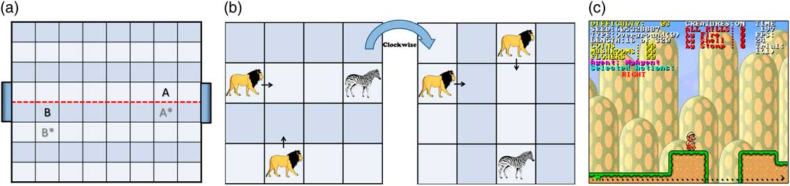
-value and therefore implicitly forces a generalization over the feature space. A common method is using a factored state-space representation, where each state is represented by a vector of features that capture different characteristics of the state-space. Using such abstraction, one can define similarities using an index over the factored state–action (e.g. Sequeira et al., Reference Sequeira, Melo and Paiva2013; Brys et al., Reference Brys, Harutyunyan, Suay, Chernova, Taylor and Nowé2015). Defining representational similarities introduces the major engineering concern of choosing the right abstraction method or FA that would work well across the entire state–action space, while minimizing generalizing between dissimilar state–actions. Representational similarity has repeatedly shown its benefit in real-world applications, but no one-size-fits-all method exists for efficiently representing the state–action space. See Figure 1 (a) for an illustration.2. Symmetry similarity seeks to consolidate state–action pairs that are identical or completely symmetrical in order to avoid redundancies. Zinkevich and Balch (Reference Zinkevich and Balch2001) formalized the concept of symmetry in MDPs and proved that if such consolidation of symmetrical state–actions is performed accurately, then the optimal
$Q$
function and the optimal policy are not altered. However, automatically identifying symmetries is computationally complex (Narayanamurthy & Ravindran, Reference Narayanamurthy and Ravindran2008), especially when the symmetry is only assumed. For example, in the Pursuit domain, one may consider the 90°, 180° and 270° transpositions of the state around its center (along with the direction of the action) as being similar (see Figure 1 (b)). However, as the predators do not know the prey’s (potentially biased) policy, they can only assume such symmetry exists.3. Transition similarity can be defined based on the idea of relative effects of actions in different states. A relative effect is a change in the state’s features caused by the execution of an action. Exploiting relative effects to speed up learning was proposed (Jong & Stone, Reference Jong and Stone2007; Leffler et al., Reference Leffler, Littman and Edmunds2007) in the context of model learning. For example, in the Mario domain, if Mario walks right or runs right, outcomes are assumed to be similar as both actions induce similar relative changes to the state (see Figure 1(c)). In environments with complex or non-obvious transition models, it can be difficult to intuit this type of similarity.


(a) Players in the simple robotic soccer task are A and B; the state in which the two players are moved one cell down (A* and B*) should be considered similar. (b) Two (presumed) similar state–action pairs in the Pursuit domain. (c) A state in the Mario task where walking or running right are considered similar (i.e. falling into the gap)

3.1 SASS in the
$Q$
-learning framework

We use the designer-provided similarity function σ(s, a, s′, a′) instead of the spreading function needed by the
 $QS$
-learning algorithm (as discussed in Section 2). In words, for each experience 〈s, a, r, s′〉 that the agent encounters, depending on the similarity function σ, we potentially update more than a single
 $\left\langle {s,\,a} \right\rangle $
entry in the
 $Q$
table. Multiple updates, one for each entry
 $\left\langle {\tilde{s},\,\tilde{a}} \right\rangle $
for which
 $$\sigma (s,\,a,\,\tilde{s},\,\tilde{a})\,\gt\,0$$
, are performed using the following update:
 $$Q(\tilde{s},\,\tilde{a}){\equals}Q(\tilde{s},\,\tilde{a}){\plus}\alpha \sigma (s,\,a,\,\tilde{s},\,\tilde{a})\delta $$
which, as discussed in Section 2, does not compromise the theoretical guarantees of the unadorned
 $Q$
-learning.
The update rule states that as a consequence of experiencing 〈s, a, r, s′〉, an update is made to other pairs
 $\left\langle {\tilde{s},\,\tilde{a}} \right\rangle $
as if the real experience was actually
 $\left\langle {\tilde{s},\,\tilde{a},\,r,\,s'} \right\rangle $
(discounted by the similarity function).
In order to avoid a time complexity of O(|S||A|) per step,
 $QS$
-learning should be restricted to update state–action pairs for which the similarity is larger than 0. In our experiments (see Section 4) we found only a minor increase in time-complexity for most human-provided similarity functions.
In the interest of clarity, from this point forward we will use the term
 $QS$
-learning using the above Q-learning-with-SASS interpretation. Namely, using a designer-defined similarity function σ and the update rule of Equation (2), we will modify the classic
 $QS$
-learning algorithm yet keep its original name due to their inherent resemblance. See Algorithm 1 for the QS-learning Algorithm as used in this study.

4 Evaluation
Our human subject study is comprised of three experimental settings: first, we examine the SASS approach against a baseline learner (i.e. no speedup method) and the FA approach in the simple robotic soccer task with 16 non-expert developers. Through this experiment, which we will refer to as Experiment 1, we show the potential benefits of the SASS approach compared to FA given basic, classic RS taken from previous works. Next, we evaluate all three speedup approaches (FA, RS and SASS) along with a baseline learner using the Pursuit and Mario tasks. Through this experiment, which we will refer to as Experiment 2, we find that RS provides the most natural approach of the three for most non-expert developers. However, the results further show that the combination of RS and SASS (as was tested in Experiment 1) can bring about significant potential benefits with minimal overhead effort. Lastly, in Experiment 3, we evaluate all three tasks using three expert developers. The results support our findings in Experiments 1 and 2, demonstrating high effectiveness for the combination of RS and SASS compared to the individual use of each approach.
Throughout this section, we will use the following notations: a basic Q-learning agent is denoted Q, a QS-learning agent is denoted QS, a Q-learning agent that uses state-space abstraction is denoted QA, a Q-learning agent that uses RS is denoted QR and an agent which combines RS and similarities is denoted QRS.
We first discuss the three domains we tested in this study followed by the three experiments.
4.1 Evaluated domains
4.1.1 Simple robotic soccer
Proposed in Littman (Reference Littman1994), the task is performed on an 8×8 grid world, defining the state-space S. Two simulated robotic players occupy distinct cells on the grid and can either move in one of the four cardinal directions or stay in place (five actions each). The simulated robots are designed to play a simplified version of soccer: At the beginning of each game, players are positioned according to Figure 1(a) and possession of the ball is assigned to one of the players (either the learning agent or the fixed, hand-coded policy opponentFootnote 2 ). During each turn, both players select their actions simultaneously and the actions are executed in random order. When the attacking player (the player with the ball) executes an action that would take it to a square occupied by the other player, possession of the ball goes to the defender (the player without the ball) and the move does not take place. A goal is scored when the player with the ball enters the other player’s goal region. Once a goal is scored the game is won; the agent who scored receives 1 point, the other agent receives −1 point and the game is reset. The discount factor was set to 0.9, as in the original paper.
We used a basic state-space representation, as done in Martins and Bianchi (Reference Martins and Bianchi2013), a recent investigation of the game. A state s is represented as a 5-tuple 〈x A , y A , x B , y B , b〉 where x i and y i indicate player i’s position on the grid and b∈{A, B} indicates which player has the ball. The action-space is defined as a set of five actions as specified above. Overall, the state–action space consists of ~41000 state–action pairs (84(locations)×2(ball−possession)×5(actions)).
4.1.2 Pursuit
The Pursuit task (also known as Chase or Predator/Prey task) was proposed by Benda (Reference Benda1985). For our evaluation, we use the recently evaluated instantiation of Pursuit implemented in Brys et al. (Reference Brys, Nowé, Kudenko and Taylor2014). According to the authors’ implementation, there are two predators (Pred
1, Pred
2) and one prey (Prey), each of which can move in one of the four cardinal directions as well as stay in place (five actions each) on a 20×20 grid world. The prey is caught when a predator moves onto the same grid cell as the prey. In that case, a reward of 1 is given to the predator, 0 otherwise. A state s is represented as a 4-tuple
 $$\left\langle {\Delta _{{x_{1} }} ,\,\Delta _{{y_{1} }} ,\,\Delta _{{x_{2} }} ,\,\Delta _{{y_{2} }} } \right\rangle $$
where
 $\Delta _{{x_{i} }} $
 ${(\Delta _{{y_{i} }})} $
is the difference between predator i’s x-index (y-index) and the prey’s x-index (y-index). Overall, the state–action space consists of approximately 46 million state–action pairs (394(differences)×20(actions)).
4.1.3 Mario
Super Mario Bros is a popular two-dimensional side-scrolling video game developed by the Nintendo Corporation. This popular game is often used for the evaluation of RL techniques (Karakovskiy & Togelius, Reference Karakovskiy and Togelius2012). In the game, the player’s figure, Mario, seeks to rescue the princess while avoiding obstacles, fighting enemies and collecting coins. We use the recently evaluated formulation of the Mario task proposed by Suay et al. (Reference Suay, Brys, Taylor and Chernova2016). The authors use a 27-dimensional discrete state-variables representation of the state-space and model 12 actions that Mario can take. We refer the reader to the original paper for the complete description of the underlying MDP and parameters. Given the authors’ abstraction of the state-space, the size of the state–action space is over 100 billion, although many of the possible states are never encountered in reality. For example, it is impossible to have Mario trapped by enemies from all directions at the same time. Due to the huge state–action space, and unlike the Simple Robotic Soccer and Pursuit tasks, a condition where
 $Q$
-learning is evaluated without the authors’ abstraction will not be evaluated.
In the Pursuit and Mario tasks, we use
 $Q(\lambda )$
-learning and
 $QS(\lambda )$
-learning, which are slight variations of the
 $Q$
-learning and
 $QS$
-learning algorithms that use eligibility traces (Sutton & Barto, Reference Sutton and Barto1998). The addition of eligibility traces to the evaluation was carried out as done by the authors of the recent papers from which the implementations have been taken, namely Brys et al. (Reference Brys, Nowé, Kudenko and Taylor2014) and Suay et al. (Reference Suay, Brys, Taylor and Chernova2016). This allows us to evaluate the different approaches with recently provided baseline solutions without altering their implementations.
4.2 Experiment 1: initial non-expert developers study
In this experiment, we seek to investigate the potential benefits of the SASS approach. We focus on technically able non-experts with some background in programming and RL. We speculate that participants would find the SASS approach more appealing than the FA approach which in turn will result in designers’
 $QS$
agents outperforming the designers’
 $QA$
agents. To examine this hypothesis, we recruited 16 Computer Science graduate-students majoring in AI—four PhD students and 12 Masters students, ranging in age from 23 to 43 (average of 26.8), 10 males and six females—to participate in the experiment and act as non-expert designers for two RL agents (
 $QS$
and
 $QA$
). All participants have some prior knowledge of RL from advanced AI courses (about two lectures) yet they cannot be considered experts in the field as they have no significant hands-on experience in developing RL agents. The students are majoring in Machine Learning (7), Robotics (4) and other computational AI sub-fields (5).
We chose to start with the Simple Robotic Soccer domain, which is the simplest of the three evaluation domains in this study. Prior to the experiment, all subjects participated in an hour-long tutorial reminding them of the basics of
 $Q$
-learning and explaining the Simple Robotic Soccer task’s specification. The tutorial was given by the first author of this article, an experienced lecturer and tutor. Participants were then given two python codes: first, an implemented
 $QA$
agent for which participants had to design and implement a state-space abstraction. Specifically, the participants were requested to implement a single function that translates the nave representation of the state-space to their own state-space representation. Second, participants were given a
 $QS$
agent for which they had to implement a similarity function. Both codes already implemented all of the needed mechanisms of the game and the learning agents, and they are available at http://www.biu-ai.com/RL
In order to allow the participants to evaluate their agent’s performance in reasonable time, a basic RS was implemented under both conditions (
 $QA$
and
 $QS$
) as suggested in the original Simple Robotic Soccer paper (Littman, Reference Littman1994). The suggested RS is of a PBRS structure (Ng et al., Reference Ng, Harada and Russell1999), biasing the player to move toward the goal while on offense and toward the other player while on defense. It is important to note that the use of PBRS allows one to modify the reward function without altering the desired theoretical properties of
 $Q$
-learning and
 $QS$
-learning algorithms.
We used a within-subjects experimental design where each participant was asked to participate in the task twice, a week apart. In both sessions, the participants’ task was to design a learning agent that would outperform a basic
 $Q$
agent in terms of asymptotic performance and/or average performance (one would suffice to consider the task successful) by using either abstraction or similarities, in no more than 45 minutes of work. Ideally, we would want participants to take as much time as they need. However, given that each participant had to dedicate about 3 hours for the experiment (a one hour tutorial, 1.5 hours of programming and half an hour of logistics) we could not ask participants for more than 45 minutes per condition. Participants were counter-balanced as to which method they were asked to implement first. After each session, subjects were asked to answer a NASA Task Load Index (TLX) questionnaire (Hart & Staveland, Reference Hart and Staveland1988).
In order to ensure the scientific integrity of the submitted agents, participants were requested to perform the task in our lab, in a quiet room, using a designated Linux machine which we prepared for them. Furthermore, while programming, a lab assistant (who did not co-author this article) was present to assist with any technical issues. No significant technical difficulties were encountered that might jeopardize the results.
We then tested the participant’s submitted agents against the same hand-coded opponent against whom they had trained. During each session, participants could test the quality of their designed agent at any time by running the testing procedure, which worked as follows: the designed agent was trained for 1000 games such that after each batch of 50 games, the learning was halted and 10000 test games were played during which no learning occurred. The winning ratio for these 10000 test games was presented to the designer after each batch. Given a ‘reasonable’ number of updates per step (i.e. dozens to hundreds), the procedure does not take more than a few seconds on a standard PC. In order to allow designers to compare their agents’ success to a basic
 $$Q$$
agent (the benchmark agent they were requested to outperform), each designer was given a report on a basic
 $$Q$$
agent that was trained and tested prior to the experiment using the same procedure described above. After all agents were submitted, each agent was tested and received two scores: one for its average performance during its learning period and one for the asymptotic performance of the agent, that is, its performance after the training is completed. For this evaluation, we used the same machine used by the study participants, a Linux machine with 16 GB RAM and a CPU with four cores, each operating at 4 GHz. Each agent was evaluated 50 times over 1000 episodes, so the score of each episode is in fact an average of the 50 evaluation runs.
4.2.1 Results
Under the
 $QS$
-learning condition, participants defined similarity functions. A similarity function is beneficial only if it helps the
 $QS$
agent outperform the basic
 $Q$
agent. Otherwise, we say that the similarity function is flawed in that it hinders learning.
When analyzing the average performance of the submitted agents, we see that out of the 16 submitted
 $QS$
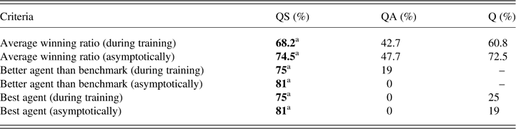
agents, 12 (75%) successfully used a beneficial similarity function. On the other hand, only three (19%) of the 16
 $QA$
agents outperformed the
 $$Q$$
agent. The average winning ratio recorded for the
 $QS$
agents throughout their training was 68.2%, compared to the 42.7% averaged by the
 $QA$
agent and 60.8% averaged by the benchmark
 $Q$
agent.
Asymptotically, 13 out of the 16
 $QS$
agents (81%) outperformed or matched the basic
 $Q$
agent performance. None of the
 $QA$
agents asymptotically outperformed the
 $Q$
agent. On average, under the
 $$QS$$
-learning condition, participants designed agents that asymptotically achieved an average winning ratio of 74.5%. The
 $QA$
agents achieved only 47.7% and the
 $Q$
agent recorded 72.5%.
Interestingly, all 16 participants submitted
 $QS$
agents which perform better than their submitted
 $QA$
agents both in terms of average learning performance and asymptotic performance. Namely, the
 $QS$
agents’ advantage over the
 $$QA$$
agents is most apparent when examining each designer separately. Furthermore, for all participants, the
 $QS$
agent outperforms the
 $QA$
agent from the third test (the 150th game) onwards. For nine of the 16 participants (56%), the
 $QS$
agent outperformed the
 $QA$
agent from the very first test onwards. In addition, the
 $$QS$$
agents completed the learning period faster than the
 $$QA$$
agents on average, which may imply that a beneficial SASS-based logic is less complex than a FA-based one.
We further analyzed the types of similarities that participants defined under the
 $QS$
-learning condition. This phase was done manually by the authors, examining the participants’ codes and trying to reverse-engineer their intentions. Fortunately, due to the task’s simple representation and dynamics, distinguishing between the different similarity notions was possible. It turns out that representational and symmetry similarity notions were the most prevalent among the submitted agents. In eight of the 16
 $QS$
agents (50%), representational similarities were instantiated, mainly by moving one or both of the virtual players across the grid, assuming that the further away one moves the player(s), the lower the similarity is to the original positioning (see Figure 1(a)). Symmetry similarities were used by 7 of the 16 participants (43.7%). All 7 of these agents used the idea of mirroring, where the state and action were mirrored across an imaginary horizontal line dividing the grid in half. Some of them also defined mirroring across an imaginary vertical line dividing the grid in half, with an additional change of switching ball position between the players. While we were able to show that each of these ideas is empirically beneficial on its own, we did not find evidence that combining them brings about a significant change. Transitional similarities were only defined by two of the 16 participants (12.5%). Both of these designers tried to consider a more strategic approach. For instance, moving toward the opponent while on defense is considered similar, regardless of the initial position. It turns out that neither of the provided transitional similarities were beneficial on their own as they were submitted by the designers.
Only four of the 16 participants (25%) used more than a single similarity notion while defining the similarity function. Interestingly, the two best performing
 $QS$
agents combined two notions in their similarity function (representational and symmetry similarities). We speculate that combining more than a single similarity notion can be useful for some designers, yet in the interest of keeping with the task’s tight time frame, participants refrained from exploring too many different directions and focused on the ones they initially believed to be the most promising.
Recall that four participants (25%) submitted flawed similarity functions. Although these participants were unable to find a beneficial similarity function, the submitted
 $QS$
agents were not considerably worse than the basic
 $Q$
-learning. The average performance for these four agents was 56.9% compared to 60.8% for the basic
 $$Q$$
agent, and their average asymptotic score was 61.5% compared to 72.5% for the basic
 $$Q$$
agent.
Unlike the significant difference between the
 $QA$
-learning and
 $QS$
-learning conditions in terms of agents’ performance, a much larger number of participants is needed to achieve significant results in terms of TLX scores. Using the analysis of variance (ANOVA) one-way test on the experiment results we find an F-ratio of 1.5093 and a p-value of 0.2282, which do not reflect a significant difference. The complete TLX results are available at http://www.biu-ai.com/RL
Overall, the results are aligned with our initial hypothesis and demonstrate that designers better utilized the SASS approach compared to the FA approach. The results are summarized in Table 1.
Experiment 1 main results summary

a (p < 0.05).
The main results of Experiment 1 (non-expert study). The results show that the State Action Similarity Solutions approach allowed most designers to outperform the basic
 $Q$
-learning condition and better infuse their domain-knowledge into the reinforcement learning agent compared to the function approximation approach. The higher the score—the better.
4.3 Experiment 2: non-expert developers study
In Experiment 2 we seek to investigate three speedup methods: FA, RS and SASS. Similar to Experiment 1, we speculate that participants would be able utilize the SASS approach and produce agents which outperform the QA and Q agents. In addition, we speculate that RS would also be successfully utilized by designers to outperform the QA and Q agents. We again focus on technically able non-expert designers who have a strong background in programming yet a very limited experience with RL. Similar to Experiment 1, we required 32 human participants, all of whom were senior Bachelors or beginning graduate students who are majoring in AI and have participated in an advanced AI course. The participants ranged in age from 20 to 50 (average of 27.2), 23 male and nine female. The students are majoring in Machine Learning (22), Robotics (7) and other computational AI sub-fields (3). None of the participants in this experiment participated in Experiment 1.
Unlike Experiment 1, in this experiment we investigate two more complex RL tasks: Pursuit and Mario. First, we randomly assigned each participant to one of two equally sized groups. Each group was assigned a different domain; either Pursuit or Mario. Similar to Experiment 1, participants were given three Java codes: an implemented
 $QA$
agent for which participants had to design and implement a state-space abstraction, a
 $QS$
agent for which participants had to implement a similarity function, and a
 $QR$
agent for which participants had to implement a RS function. Note that the last condition (
 $QR$
-learning) was not present in Experiment 1 as a basic shaping reward was already implemented as discussed in Section 4.2. All codes had already implemented all of the needed mechanisms of the game and the learning agents, and they are available at http://www.biu-ai.com/RL. It is important to stress that, unlike Experiment 1, we provided no basic RS for the agents.
We again use a within-subjects experimental design where each participant was asked to participate in the task thrice, with a week separating every two consecutive conditions. Due to the increased complexity of the two domains tested in this experiment compared to Experiment 1, and to allow easy reproducibility of the experiment, participants were given an interactive PowerPoint presentation that introduced the problem domain as well as reminded them of the fundamentals of the tested speedup methods instead of the 1-hour tutorial given in Experiment 1. The PowerPoint presentations are available on our website http://www.biu-ai.com/RL. As before, in all sessions, the participants’ task was to design a learning agent that would outperform a basic
 $Q$
-learning condition in terms of asymptotic performance and/or average performance (one would suffice to consider the task successful) by using either FA, SASS or RS, in no more than 45 minutes of work for each condition. In this experiment, participants had to devote about 4 hours due to the additional conditions and logistics.
Similar to Experiment 1, participants were instructed to use a designated machine in our lab and were assisted by a lab assistant in case they faced any technical difficulties. No significant technical difficulties were encountered that might jeopardize the results.
Participants were counter-balanced as to which agent they had to implement first. Following each programming session, the participants were asked to answer a NASA TLX questionnaire. In addition, in order to acquire a better understanding of participants’ subjective experience, an additional short questionnaire was administered. The questionnaire consisted of nine statements to which participants had to rate the degree to which each statement reflects their subjective feeling on a 10-point Likert scale. For instance, ‘To what extent was the speedup method you used appropriate for the task you were required to complete?’. The complete questionnaire is available on our website—http://www.biu-ai.com/RL. The four key questions, which we will discuss here, can be found in Appendix A. During each session, participants could test the quality of their agent by running the following testing procedure: in the Pursuit task, the agent trained for 100000 games, where after each batch of 100 games the average performance of the agent within that batch was presented graphically to the designer. In the Mario task, the agent was trained for 7500 games, where after each batch of 100 games the average performance of the agent within that batch was presented graphically to the designer. The above procedure is slightly different from Experiment 1 due to time considerations: for the Pursuit task, most submitted agents completed 100000 training games in no more than a few seconds on a standard PC. On the other hand, for the more complex Mario task, the test procedure took up to half a minute despite the limited training duration of only 7500 games.
In order to allow designers to compare their agents’ success to a basic
 $Q$
-learning condition (the benchmark agent which they were requested to outperform), each designer was given a report on the performance of a basic
 $Q$
agent that was trained and tested prior to the experiment using the same procedure described above.
For evaluation, we used the same machine used by the study participants, a Windows machine with 12 GB of RAM and a CPU with eight cores, each operating at 3 GHz.
In addition to the evaluation of the three methods that each designer developed during this experiment, we evaluated an additional condition. We manually combined each of the developers’
 $QR$
agents with his or her
 $QS$
agent, resulting in a new agent which we called
 $Q$
agent. Note that each of the resulting
 $QRS$
agents uses both the RS and similarity implementations of a specific participant. The
 $QRS$
agents are similar in spirit to the
 $QS$
agents from Experiment 1, as RS was also implemented for these agents. It is important to mention that participants developed each agent independently and were not informed about this future combination of the
 $QS$
and
 $QR$
agents. In total, 128 agents were evaluated for the two domains combined (32 participants, four agents each).
Recall that in the Pursuit and Mario tasks, we use
 $Q(\lambda )$
-learning and
 $QS(\lambda )$
-learning, which are slight variations of the
 $Q$
-learning and
 $QS$
-learning algorithms that use eligibility traces.
4.3.1 Results
We report the results for each group separately.
4.3.1.1 Pursuit
Recall that a submitted agent is considered successful if it outperforms the basic
 $Q$
agent in at least one of the two criteria of interest: average performance or asymptotic performance. In the Pursuit task, the score is the number of steps required by both predators to catch the prey. As a result, it is important to remember that the lower the score, the better.
When analyzing the average performance of the submitted agents, we see that out of the 16 submitted
 $QS$
agents, 14 (87.5%) successfully used a beneficial similarity function. Similar to the results of Experiment 1, very few of the submitted
 $QA$
agents (4 out of 16, 25.0%) were able to outperform the basic
 $Q$
-learning condition. When examining the submitted
 $QR$
agents, we see similar results to the
 $QS$
-learning condition, with 15 out of the 16 submitted agents (93.75%) outperforming the
 $Q$
-learning condition. As for the
 $QRS$
agents, 14 out of the 16 agents (87.5%) were successful, similar to the
 $QS$
-learning condition. The
 $QS$
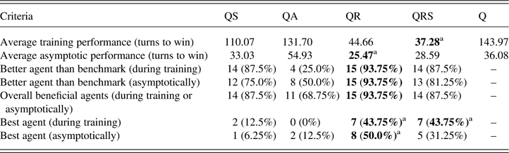
agents achieved an average training score of 110.07, outperforming the
 $QA$
agents and the
 $Q$
-learning baseline which scored 131.7 and 143.91, respectively. Interestingly, the
 $QR$
agents averaged a score of 44.66, less than half of what the
 $QS$
agents averaged. However, in the
 $QRS$
-learning condition, where we manually combined the
 $QS$
and
 $QR$
agents of each study participant, the resulted agent averaged a score 37.28, reducing the
 $QR$
-learning condition average by 16.5% and the
 $QS$
-learning condition average by 66%.
Evaluating the asymptotic performance of the agents reveals similar results: out of the 16
 $QS$
agents, 12 outperformed or matched the basic
 $Q$
-learning condition performance (75.0%), averaging 33.03 compared to the asymptotic score of 36.08 by the
 $Q$
agent. Only eight of the 16
 $QA$
agents (50.0%) were able to achieve the same, averaging 54.93. Almost all of the submitted
 $QR$
agents were able to outperform the basic
 $Q$
agent (15 out of 16, 93.75%), averaging 25.47. The
 $QRS$
agents were suited between the
 $QS$
-learning and
 $QR$
-learning conditions, with 13 successful agents out of 16 (81.25%), averaging 28.5.
Interestingly, all
 $QS$
,
 $QR$
and
 $QRS$
agents that outperformed the
 $Q$
-learning condition on the criteria of average training performance managed to outperform the
 $Q$
-learning condition asymptotically as well. Surprisingly, this does not hold for any of the
 $QA$
agents.
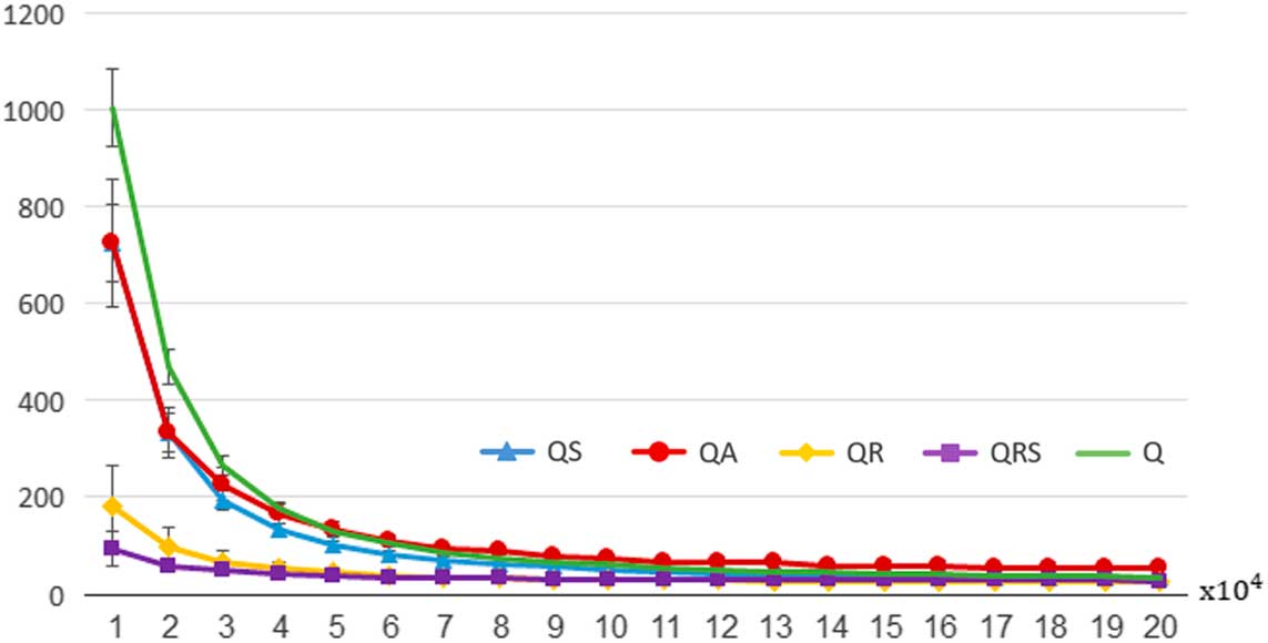
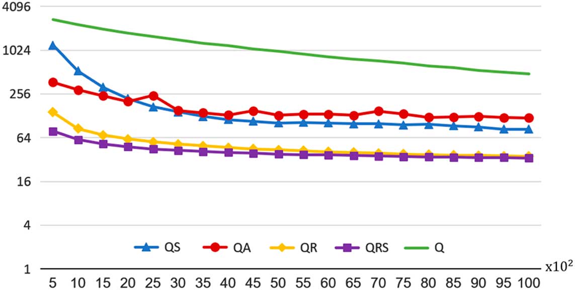
The results are summarized in Table 2 and illustrated in Figure 2.
Pursuit agents’ average learning curves under the examined conditions. The x-axis marks the number of training games. The y-axis marks the average game score. The lower the score—the better. Error bars indicate standard error

Summary of Experiment 2 main results: Pursuit task

a (p < 0.05).
The main results of Experiment 2 (non-expert study). The results show that the State Action Similarity Solutions and reward shaping approaches allow most designers to outperform the basic
 $Q$
-learning condition and better infuse their domain-knowledge into the reinforcement learning agent compared to the function approximation approach. The results further show that the
 $QR$
-learning condition consistently outperforms the
 $QS$
-learning condition while the combination of the two,
 $QRS$
-learning, is found to improve the agent’s average performance during training for most cases. The lower the score—the better.
Only nine out of the 128 agents (7%) were flawed (2
 $QS$
agents, 5
 $QA$
agents, a single
 $QR$
agent and a single
 $QRS$
agent). In Experiment 1, flawed agents did not perform significantly worse than the baseline
 $Q$
-learning condition. However, in Experiment 2, flawed agents performed quite poorly, scoring an average and asymptotic performance between 4 and 120 times worse than the baseline
 $Q$
-learning condition.
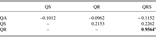
Interestingly, a strong correlation was observed between agents’ average performance under the
 $QR$
-learning and
 $QRS$
-learning conditions (0.96), whereas a correlation of only 0.22 was found between the
 $QS$
-learning and
 $QRS$
-learning conditions. Very weak negative correlations were found between the
 $QA$
agents’ performance and other agents (−0.1 with
 $QS$
agents and
 $QR$
agents and −0.12 with the
 $QRS$
agents). A weak correlation was observed between the
 $QS$
agents and the
 $QR$
conditions (0.22). These results suggest that participants who were successful with one method were not necessarily successful with others. The only exception to the above claim is the
 $QR$
-learning condition, which seems to bear the most effect on the
 $QRS$
-learning condition as they are almost perfectly correlated. Results are summarized in Table 3.
Correlation between agent types in Experiment 2: Pursuit task

a (p < 0.05).
A strong positive correlation exists between the number of valid agents in the QR and QRS learning conditions.
Considering each participant individually, we find that for seven participants out of 16 (43.8%) the best-performing agent, in terms of average performance, was the
 $QRS$
agent. For an additional seven participants (43.8%), the best-performing agent was the
 $QR$
agent. For the remaining two participants, the best-performing agent was the
 $QS$
agent. Consistent with the results of Experiment 1, the
 $QA$
agent was not the best-performing agent for any of the participants. Deeper head-to-head analysis reveals similar trends—12 participants developed a
 $QS$
agent which outperformed their
 $QA$
agent (75%) and 13 participants developed
 $QR$
and
 $QRS$
agents which outperform their
 $QS$
agent (81.3%). For eight participants (50%) the combination of the
 $QS$
and
 $QR$
agents—the
 $QRS$
agent—outperformed both their
 $QR$
and
 $QS$
agents.
As for the asymptotic performance of the tested agents, we find that for eight participants out of 16 (50.0%) the best-performing agent was the
 $QR$
agent. For an additional five participants (31.25%), the best-performing agent was the
 $QRS$
agent. For only two participants the best-performing agent was the
 $QA$
agent and for only a single one the best-performing was the
 $QS$
agent. Consistent with the above results, a head-to-head analysis reveals similar trends—11 participants developed a
 $QS$
agent which outperformed their
 $QA$
agent (68.75%) and 13 participants developed
 $QR$
and
 $QRS$
agents which outperform their
 $QA$
agent (81.3%). For 10 participants (62.5%) the combination of the
 $QS$
and
 $QR$
agents—the
 $QRS$
agent—outperformed both their
 $QR$
and
 $QS$
agents.
We further analyze the types of similarities and RS functions that participants defined under the
 $QS$
-learning and
 $QR$
-learning conditions. This phase was done manually by the authors, examining the participants’ codes and attempting to reverse-engineer their intentions. Under the
 $QS$
-learning condition, and contrary to what one may expect, only a single participant instantiated representational similarities. This may be partially attributed to the less-trivial representation of the state-space (i.e. using differences instead of absolute x, y locations) as implemented in the original paper. Symmetry similarities were used by five out of the 16 participants (31.3%), four of whom used angular rotations with 90°, 180° and 270° transpositions of the state around its center (along with the direction of the action, see Figure 1(b) for an illustration), and three of which used mirroring (two used both). Interestingly, nine out of 16 participants (56.3%) defined transitional similarities, considering all state–action pairs which are expected to result in the same state. Under the
 $QR$
-learning condition, most participants (14 out of 16, 87.5%) developed agents based on motivating the predators to move toward the prey and discouraging them from moving in any other direction. This simple idea was shown to be highly effective, as depicted by the scores discussed above. The remaining two participants also rewarded the predators based on the separation between the predators (intuitively, rewarding the predators for avoiding interfering with each other’s moves). This addition had mixed effects on the agent’s performance.
Considering the participants’ TLX scores, using a one-way ANOVA test we find that the scores are significantly different (F=6.79348, p<0.05). Using post-hoc analysis, we find that the TLX results of both the
 $QA$
-learning and
 $QR$
-learning conditions are not significantly different. However, the
 $QS$
-learning condition was found to have higher mean TLX scores compared to both the
 $QA$
-learning and
 $QR$
-learning conditions (p<0.05). These results indicate that articulating similarities in the Pursuit domain demands higher levels of developers’ effort compared to articulating RS or basic FA. The full TLX results and tests results can be found on the project’s webpage http://www.biu-ai.com/RL
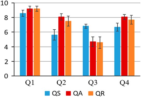
In addition to the TLX questionnaire, we administered a customized questionnaire that aims at extracting the participants’ subjective experience during the experiment. The English version of the questionnaire can be found in Appendix A. Participants’ answers demonstrate a few interesting phenomena: first, participants reported that they understand their task requirements and purpose well (
 $Q_{1} $
in Appendix A, averaging nine out of 10), with no statistically significant difference between the different conditions. Interestingly, participants reported that the
 $QS$
-learning condition was the most challenging (
 $Q_{2} $
in Appendix A, averaging 5.6 compared to 8.1 and 7.5 under the
 $QA$
-learning and
 $QR$
-learning conditions, respectively, p<0.05. There was no statistically significant difference between the latter pair.). See Figure 3 for graphical representation. We find support for the above in the participants’ TLX scores: the
 $QS$
-learning condition was shown to induce a higher mental demand (averaging 71.25 compared to 59.68 and 44.37 for the
 $QA$
-learning and
 $QR$
-learning conditions, respectively. Here, the difference between the
 $QA$
-learning and
 $QR$
-learning conditions was found to be statistically significant as well, p<0.05.). On the other hand, participants reported that under the
 $QS$
-learning condition they could have improved the agent’s performance much more if they were to be given more time (
 $$Q_{3} $$
in Appendix A, averaging 6.8 compared to 4.6 and 4.5 under the
 $QA$
-learning and
 $QR$
-learning conditions, respectively, p<0.05. There was no statistically significant difference between the latter pair.). This is also supported by participants reporting extremely high time pressure under the
 $QS$
-learning condition, as reflected by the Temporal Demand index of their TLX scores (averaging 74.37 compared to 43.43 and 38.43 for the
 $QA$
-learning and
 $QR$
-learning conditions, respectively, p<0.05. There was no statistically significant difference between the latter pair.).
Pursuit post-experiment customized questionnaire average answers. See Appendix A for details

The above results combine to suggest that the
 $QA$
-learning and
 $QR$
-learning methods were more natural for human designers for the pursuit task, given the imposed time limit. This insight is also aligned with participants reporting the
 $QS$
-learning condition as the least appropriate method for the pursuit task (
 $Q_{4} $
in Appendix A, averaging 5.7 compared to 7.3 and 7.1 under the
 $QA$
-learning and
 $QR$
-learning conditions, respectively, p<0.05. There was no statistically significant difference between the latter pair.). The full TLX scores and participants’ answers are available at http://www.biu-ai.com/RL
4.3.1.2 Mario
As before, a submitted agent is considered successful if it outperforms the basic
 $Q$
agent in at least one of the two criteria: average performance or asymptotic performance. Unfortunately, the vast majority of submitted Mario playing agents were flawed (71%). Specifically, 13 out of the 16
 $QS$
agents (81.3%), 10 out of the 16
 $QA$
agents (62.5%) and 11 out of the 16
 $QR$
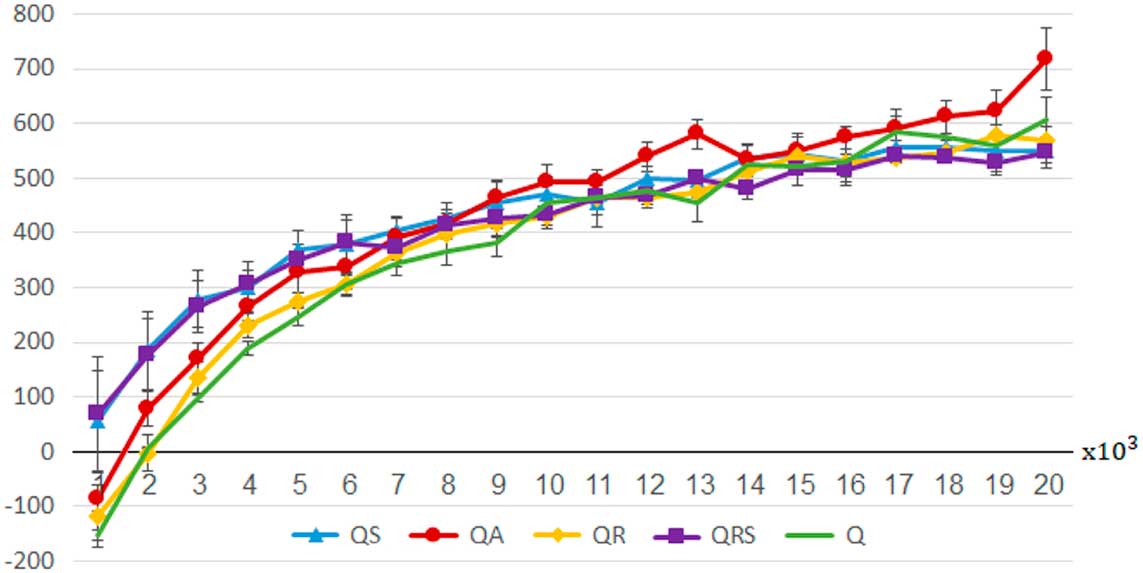
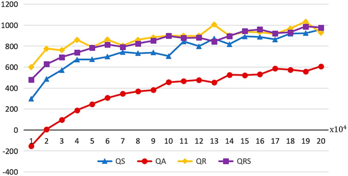
agents (68.8%) were flawed. The average learning curves of the different conditions are illustrated in Figure 4.
Mario agents’ average learning curves under the examined conditions. The x-axis marks the number of training games. The y-axis marks the average game score. The higher the score—the better. Error bars indicate standard error

The only significant result in this context is the superiority of the
 $QS$
agents over the
 $Q$
-learning baseline in the first four batches of learning. While the
 $QS$
agents outperform the
 $QA$
,
 $QR$
and
 $QRS$
agents, it is important to note that they are all superseded by the baseline
 $Q$
-learning condition on average.
It is uncommon for AI articles to report negative results. Nevertheless, we believe that some useful lessons can be learned from this part of the experiment. Specifically, the answers from participant questionnaires’ can shed light on the results. First, participants reported that they understand their task requirements and purpose well (
 $$Q_{1} $$
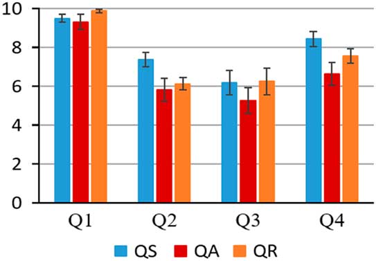
in Appendix A, averaging 9.5). Thus, a lack of understanding was not the problem in our case. Participants further indicated that they could significantly improve their agent’s performance if they were given more time (
 $$Q_{3} $$
, averaging 6.2 with no significant differences between the conditions). Given the participants’ answers, also supported by short, informal interviews we conducted with participants after the experiment, we speculate that the imposed time constraint was the main catalyst for developing flawed agents. It is important to note in this context that the Mario task is significantly more complex than Simple Robotic Soccer or Pursuit in both state–action space and the game dynamics. As a result, participants are likely to require more time to come up with beneficial ideas (taking into account the complex game dynamics) and more time to instantiate different ideas (given the complex state–action space). Moreover, as noted before, Mario’s testing procedure took up to half a minute compared to a few seconds in previous tasks. This alone reduced the development time significantly as participants spent a total of a few minutes waiting for results during their already limited development time. For concreteness, consider the following example: In the Pursuit task, a simple RS function biasing the predators to move closer to the prey performed very well. Here, biasing Mario to move toward the princess (move right) does not work well as Mario has to avoid colliding with enemies, falling into gaps and he needs to try to collect coins. Designing such a complex RS function and implementing it may take significantly longer than the simplistic one in Pursuit. Furthermore, testing it would take significantly more time. We find additional support for this hypothesis in Experiment 3 (Section 4.4), where the human expert designer reported significantly more time needed to develop beneficial agents for the Mario task compared to the Simple Robotic Soccer and Pursuit domains.
Interestingly, despite the discouraging results described above, participants reported that the
 $QS$
-learning condition was the least challenging (
 $Q_{2} $
in Appendix A, averaging 7.4 compared to 6.1 and 5.8 under the
 $QA$
-learning and
 $QR$
-learning conditions, respectively, p<0.05. There was no statistically significant difference between the latter pair.). See Figure 5 for graphical representation.
Mario post-experiment customized questionnaire average answers. See Appendix A for details

This is further supported by participants reporting the
 $QS$
-learning condition as the least frustrating in their TLX scores (averaging 40.62 compared to 54.1 and 55.63 for the
 $QA$
-learning and
 $QR$
-learning conditions, respectively, p<0.05. There was no statistically significant difference between the latter pair.). Moreover, participants reported the
 $QS$
-learning condition as the most appropriate method for the Mario task (averaging 8.3 compared to 6.4 and 4.7 under the
 $QA$
-learning and
 $QR$
-learning conditions, respectively, p<0.05. Here, the difference between the
 $QA$
-learning and
 $QR$
-learning conditions was found to be statistically significant as well, p<0.05.).
The above results suggest that due to the complexities associated with the Mario task, the time limit was too restrictive. Nevertheless, participants were able to indicate the
 $QS$
-learning condition as the most natural and appropriate technique for this domain. Indeed, it was the only condition that was able to outperform the
 $Q$
-learning on average, yet only for the few first training batches.
When we combine the results for the Pursuit and Mario tasks, they seem to support our initial hypothesis that more
 $QS$
and
 $QR$
speedup can allow most designers to produce better performing agents compared to the FA approach. Moreover, the results also seem to imply that the RS speedup method is superior under the Pursuit domain, and its combination with the
 $QS$
may provide an additional speedup in many cases.
4.4 Experiment 3: expert developers study
Experiments 1 and 2 focused on non-expert, technically able human designers. In Experiment 3 we consider RL experts. In this experiment we seek to investigate expert use of the three speedup methods investigated before: FA, RS and SASS. To that end, we recruited three highly experienced, expert programmers with a Masters degrees in Computer Science and proven experience in RL (two of whom are 26 years old and the third is 27 years old). None of the experts co-author this paper. Each expert was asked to implement five RL agents: a basic
 $Q$
agent; a
 $QS$
agent; a
 $QA$
agent; a
 $QR$
agent; and a
 $QRS$
agent. Each expert was given a single RL task domain: Simple Robotic Soccer, Pursuit or the Mario game, as discussed in Section 4.1.
Each expert was instructed to take as much time as he needs to implement the agents yet keep track over the invested time for each condition. After all agents were submitted, the second author interviewed each expert about his subjective experience and thoughts during the experiment using a semi-structured interview (see Appendix B).
Unfortunately, we were unable to get the three experts to come to our lab. As a result, each expert used his own personal computer to program the different agents. The reported running times of the agents are based on our post-hoc evaluation using a personal Linux computer with 16 GB RAM and a CPU with four cores, each operating at 4 GHz. All technical parameters used by the three experts in this study (learning rates, exploration type, etc.) are fully specified in their codes and are available on the project’s webpage http://www.biu-ai.com/RL For each task, we discuss the implemented agents and their results, followed by the expert’s reflections on the task.
4.4.1 Simple robotic soccer
For this task, our expert is a 26–year-old male who works as a scientific programmer in one of the Israeli Universities. He completed a Masters degree (cum laude) majoring in AI and completed significant works using RL during his Masters and current works.
The expert reported that developing each of the agents required approximately 30 minutes except for the
 $QRS$
agent, which required only a few minutes given the implemented
 $QS$
and
 $QR$
agents.
The
 $QA$
agent used a simple distance-based approach, which represented each state according to the learning agent’s distance to its opponent and goal.
The
 $QS$
agent used two major similarity notions: First, representational similarities—the agent artificially moves both players together across the grid, keeping their original relative distance (see Figure 1). As the players are moved further and further away from their original positions, the similarity estimation gets exponentially lower. Second, symmetry similarities—experiences in the upper half of the field are mirrored in the bottom part by mirroring states and actions with respect to the y-axis and vice-versa. Transition similarities were not defined by the expert for this task.
The
 $QR$
agent used a shaping reward similar to the one proposed in Bianchi et al. (Reference Bianchi, Martins, Ribeiro and Costa2014).The expert defined that moving toward the goal while on offense and toward the opponent while on defense receives an extra bonus. Therefore, whenever an action is intended to change the proximity (using the Manhattan distance) to the attacker or the goal (depending on the situation), a PBRS is given.
The
 $QRS$
agent combined the main ideas of the
 $QS$
and
 $QR$
agents without introducing new ones.
4.4.1.1 Results
Each agent was trained for 2000 games. After each batch of 50 games, the learning was halted and 10000 test games were played during which no learning occurred. The process was repeated 350 times.
As expected of an expert, all submitted agents were successful (here they outperformed the baseline
 $Q$
agent in both criteria). The results further show that the
 $QR$
agent outperforms the
 $QA$
and
 $QS$
agents from the first batch up to the 19th batch, where it is outperformed by the
 $QS$
agent. Interestingly, the
 $QRS$
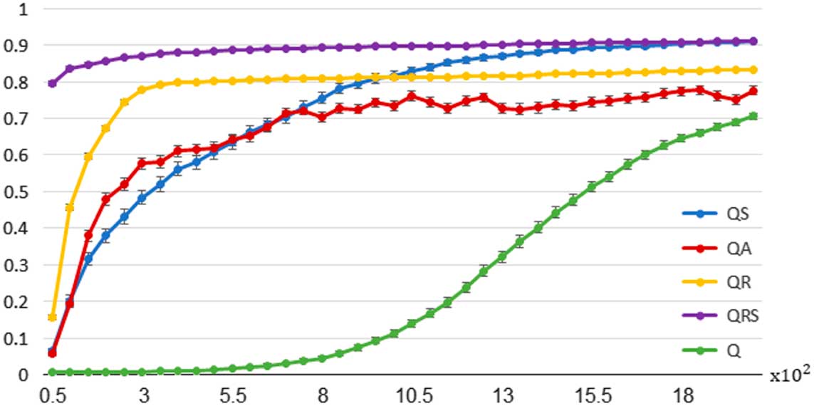
agent seems to take the best of the two, outperforming all agents from the first batch onwards. See Figure 6 for a graphical representation of the learning curves.
Soccer expert agents’ average learning curves under the examined conditions. The x-axis marks the number of training games. The y-axis marks the average game score. The higher the score—the better. Error bars indicate standard error

The evaluation of 2000 games reveals runtime differences between the conditions. The baseline condition,
 $Q$
-learning, runs the fastest, completing the evaluation in 4.5 seconds. A similar runtime was also recorded for the
 $QR$
agent. The
 $QA$
agent was a bit slower than the
 $Q$
agent, requiring about 7 seconds to complete the evaluation. The most time-consuming agents were the
 $QS$
and
 $QRS$
, requiring about 38–40 seconds each.
4.4.1.2 Expert’s reflections
The expert developed the
 $QS$
agent first, based on ideas and thoughts he had while developing the basic
 $Q$
agent. The implementation of those ideas was non-trivial, so the expert had to depend on ‘trial-and-error’ most of the time. The
 $QA$
agent was developed next. The expert claims that this method allowed him to easily translate his knowledge into code. He posits that the FA approach is most similar to the way people evaluate their surroundings before they decide which action to take. He provided the following examples: ‘On a road junction, a driver ignores most of the available information around him and focuses solely on the traffic lights’ color in order to decide whether or not to drive forward or keep still. That is what my soccer player did….’ Then, the
 $QR$
agent was developed. The expert believed that this was the most time efficient way to accelerate learning and claimed he would use RS as a first speedup tool for future tasks. Following the success of the
 $QRS$
agent, the expert claimed that the similarity notions should be considered as a ‘second-line’ speedup step.
4.4.2 Pursuit
For this task, our expert is a 27-year-old male who has worked as a senior programmer for several years. He completed a Master’s degree majoring in AI where his master’s project focused on RL.
The expert reported that developing each of the agents required approximately 3 hours, except for the
 $QRS$
agent which required about 1 hour given the implemented
 $QS$
and
 $QR$
agents.
The
 $QA$
agent was already defined by Brys et al. (Reference Brys, Nowé, Kudenko and Taylor2014) who implemented a tile-coding approximation. The expert did not see a reason to change Brys’s
 $QA$
-learning implementation. The
 $QS$
agent was defined based on angular rotations and mirroring. Each state is represented as
 $$\left\langle {\Delta _{{x_{1} }} ,\,\Delta _{{y_{1} }} ,\,\Delta _{{x_{2} }} ,\,\Delta _{{y_{2} }} } \right\rangle $$
where
 $$\Delta _{{x_{i} }} \,(\Delta _{{y_{i} }} )$$
is the difference between predator i’s x-index (y-index) and the prey’s x-index (y-index), thereby a similarity of 1 was already set for all states in which the relative positioning of the prey and predators is the same. Symmetry similarities were defined using 90°, 180° and 270° transpositions of the state around its center (along with the direction of the action, see Figure 1(b)). Furthermore, experiences in the upper (left) part of the field are mirrored in the bottom (right) part by mirroring states and actions and vice-versa. Transition similarities were defined for all state–action pairs that are expected to result in the same state.
The
 $QR$
agent was designed based on a simple logic that encourages a predator to move toward the prey and punishes moves in any other direction. The chosen shaping function returned extremely low artificial rewards (±10−22).
The
 $QRS$
agent combined the notion of symmetry from the
 $QS$
-learning condition with the
 $QR$
-learning condition. The use of angular rotations was shown to hinder the
 $QRS$
agent’s performance, and thus those were removed.
4.4.2.1 Results
Each agent was trained for 10000 games. After each batch of 100 games, the learning was halted and 10000 test games were played during which no learning occurred. The process was repeated 50 times.
Again, as one would expect of an expert, all submitted agents were successful (here they outperformed the baseline
 $Q$
agent in both criteria). The results show that the
 $QRS$
agent is the most efficient one and that it learns significantly faster than other agents. In addition, the
 $QR$
,
 $QS$
and
 $QA$
agents outperformed the baseline agent and show large improvements in the convergence rate. See Figure 7 for a graphical representation of the learning process.
Pursuit expert agents’ average learning curves under the examined conditions. The x-axis marks the number of training games. The y-axis marks the average game score in log-scale. The lower the score—the better. Standard errors are very small and thus are not noted in the figure

While the
 $Q$
,
 $QA$
and
 $QR$
agents complete their training (10000 games each) in 8.5 seconds on average (with no significant difference between the two),
 $QS$
completes the same training in 17.5 seconds on average. On average, the
 $QS$
agent updated 12 entries per iteration.
4.4.2.2 Expert’s reflections
The expert first implemented the
 $QA$
agent, followed by the
 $QS$
,
 $QR$
and
 $QRS$
agents, in that order. The expert claims that all tested methods were easy to instantiate and implement in the given domain. In terms of design effort, he sees no significant differences between the methods. He points out that under the
 $QR$
-learning condition, the first RS function he tried worked out to be the best one out of approximately a dozen functions he tested. This was not the case for the
 $QS$
agent, which he mentions to be ‘incremental’, namely the development process was a ‘step-by-step’ process where at each step a new similarity notion was introduced, evaluated and refined if needed. He believes that the
 $QS$
and
 $QR$
learning conditions are the most intuitive methods he is aware of and he recommends using them, individually or in tandem, on a task-basis. Here, he claims that the
 $QS$
-learning condition was the most appropriate. After we pointed out that the
 $QR$
agent outperformed the
 $QS$
agent he revised his answer, deeming both methods as ‘most appropriate’.
4.4.3 Mario
For this task, our expert is a 27-year-old programmer who works as a software development team leader at a large international high-tech company. He is completing a Master’s degree in Computer Science and has more than 10 years of programming experience, including work with RL.
The expert reported that developing each of the agents required a significant amount of time. The
 $QS$
agents required about 2.5 hours, whereas the
 $QR$
agent required about 2 hours. The
 $QRS$
agent required only a few minutes given the implemented
 $QS$
and
 $QR$
agents.
The
 $QA$
agent was implicitly defined by Suay et al. (Reference Suay, Brys, Taylor and Chernova2016) from which the implementation was taken. The expert did not change the given abstractions.
The
 $QS$
agent used the following representational similarity—each state representation indicates whether Mario can jump or shoot using two Boolean variables. Given a state–action pair in which Mario does not jump or shoot, all respective states (i.e. the four variations of these two Boolean variables) were defined as similar to the original pair. Namely, if Mario walks right, then regardless of Mario’s ability to shoot or jump, the state–action pair is considered similar to the original one. Symmetry similarities were defined using the mirroring of the state–actions across an imaginary horizontal line that divides the environment in half, with Mario in the middle. As illustrated in Figure 1(c), regardless of specific state, performing action a (e.g. move right) is assumed to be similar to using action a+ ‘run’ (e.g. run right). The
 $QR$
agent used the following two basic ideas: (1) moving/jumping to the right is better than moving/jumping to the left; (2) avoid getting too close to enemies and obstacles.
The
 $QRS$
agent was a simple combination of the
 $QS$
and
 $QR$
agents.
4.4.3.1 Results
Each agent was trained for 200000 games. After each batch of 10 000 games, learning was halted and 1000 test games were played during which no learning occurred. The process was repeated 50 times. The two agents are also compared to human performance level as evaluated by Suay et al. (Reference Suay, Brys, Taylor and Chernova2016). The results show that the
 $QS$
agent learns faster than the
 $QA$
agent. The
 $QR$
agent learns even faster and outperforms all other agents up to the fifth batch, when it then converges with the
 $QRS$
agent. Overall, the
 $QRS$
agent performances very similar to the
 $QR$
agent but with a slightly worse performance in the first few episodes. See Figure 8 for a graphical representation of the learning curve.
Mario expert agents’ average learning curves under the examined conditions. The x-axis marks the number of training games. The y-axis marks the average game score. The higher the score—the better. Standard errors are very small thus are not noted in the figure

4.4.3.2 Expert’s reflections
The expert developed the
 $QS$
agent first. He mentioned that due to the complex state–action space representation, significant time was invested in manipulating encountered state–action pairs in order to generate the desired similar pairs. This task was made somewhat easier when developing the
 $QR$
agent, not due to the RS technique but rather due to his experience. The
 $QR$
agent took advantage of very basic notions which the expert implemented very fast. The expert claims that the more time he put into developing better RS functions, the worse the functions turned out to be. Specifically, his best RS function was the first or second one he tried. Conversely, he mentions that this was not the case for the
 $QS$
-learning condition, in which additional similarities played a useful role in further speeding-up the RL process. He believes that the combination of RS with similarities is the most suitable for this task.
5 Conclusions
In this first-of-its-kind human study, we explored how human designers, both expert and non-expert, leverage their knowledge in order to speed up RL. We focused on the challenge of injecting human knowledge into an RL learner using the notions of abstraction, similarity and RS.
Interestingly, and contrary to its wide popularity in practice, the use of abstraction was shown to provide poor speedup results throughout the study. Specifically, in our non-expert experiments (Experiments 1 and 2), the generalization approach (represented by the
 $QA$
agents) was consistently outperformed by other conditions, and in most cases designers were unable to outperform the baseline
 $Q$
-learning condition using this approach. In our expert experiment (Experiment 3), the results present a similar trend. Specifically, participants were able to use abstraction to improve over the baseline
 $Q$
-learning, yet in all tested settings this condition came last in terms of performance. Our SASS approach, based on the notion of similarities (represented by the
 $QS$
agents), has demonstrated mixed results. In Experiments 1 and 2, it was shown to outperform the baseline
 $Q$
-learning and abstraction conditions in the vast majority of cases. However, in one of the tasks (Pursuit, Section 4.1.2) it was also shown to induce high levels of mental and temporal demand. Similar results were recorded in Experiment 3: On the one hand, the proposed method outperformed the
 $Q$
-learning and abstraction conditions. On the other hand, experts disagree on the intuitiveness of the method. It is also important to note that the method seems to require more time on the designer’s part compared to other methods. Quite consistently throughout the study, the RS condition (represented using the
 $QR$
agents) was shown to be both effective and natural for designers. Specifically, in Experiments 2 and 3, participants (both experts and non-experts) reported this technique to be the most suitable and intuitive technique, and in turn it provided superior agent performance compared to the above conditions. An exception is the Mario task in Experiment 2 (Section 4.3), where all methods performed badly, making the results hard to interpret correctly.
It turns out that the best-performing agents in this study use the combination of RS and similarities (represented by the
 $QRS$
agents). In most cases, these agents use a simple (perhaps, naïve) combination of the defined similarities under the
 $QS$
-learning conditions with the RS function defined under the
 $QR$
-learning conditions. This combination is consistently superior to the use of a single speedup method, yet it requires some development overhead since the two methods have to be implemented. Given that the two methods have already been implemented, their combination is usually straightforward and requires negligible time.
The above results combine to provide another, yet more general, insight: different techniques allow a designer to develop beneficial RL agents. However, the common ‘anecdotal proofs’ one is likely to see in RL papers illustrating the usefulness of a proposed technique (usually provided and implemented by the authors themselves) do not guarantee that the technique would be beneficial in practice with other developers and do not provide one with any ‘hint’ regarding the potential designers’ effort in implementing the proposed approach. We believe that this insight is not restricted to the challenge of injecting human knowledge into an RL learner. Thus, we hope that this work will inspire other researchers to investigate their proposed approaches and techniques in human studies, with actual programmers, to ensure the ecological validity of their contributions.
In future work, we plan to extend the proposed experimental approach to other RL algorithms (e.g. linear FA and deep RL) and techniques (e.g. learning from demonstrations). As part of this additional step, we further plan to include non-technical users, who are not expected to read or modify code, something which was not included in this study.
Acknowledgment
This article extends our previous reports from AAMAS 2017 (Rosenfeld et al., Reference Rosenfeld, Taylor and Kraus2017b) (short paper) and IJCAI 2017 (Rosenfeld et al., Reference Rosenfeld, Taylor and Kraus2017a) (full paper) in several major aspects: first, in the former, the SASS approach was presented and tested by three experts as described in Section 4.4. Then, in Rosenfeld et al. (Reference Rosenfeld, Taylor and Kraus2017a), the study was extended to include an additional 16 non-expert designers who implemented the
 $QS$
-learning and
 $QA$
-learning conditions as discussed in Experiment 1 (Section 4.2). In this article, we almost triple our participant pool by recruiting an additional 32 participants and perform an additional experiment (Experiment 2, Section 4.3). As a result of this addition, we were able to investigate the RS condition, which was not investigated in previous reports, and provide a much broader and in-depth investigation of human designers. This addition also enhances the credibility and validity of our previously reported results and demonstrates new insights which were not previously observed. An extended version of Rosenfeld et al. (Reference Rosenfeld, Taylor and Kraus2017b) entitled ‘Speeding up Tabular Reinforcement Learning Using State–Action Similarities’ was presented at the Fifteenth Adaptive Learning Agents (ALA) workshop at AAMAS 2017 and received the Best Paper Award of the workshop. This research was funded in part by MAFAT. It has also taken place at the Intelligent Robot Learning (IRL) Lab, which is supported in part by NASA NNX16CD07C, NSF IIS-1734558, and USDA 2014-67021-22174.
Appendix A: Post-experiment subjective evaluation questionnaire (Experiment 2)
1. How clear were the task requirements and purpose?
2. How complex was the task?
3. Say you were given additional time for the task. How much better do you think your agent could have become?
4. To what extent do you think that the speedup method you used is appropriate for the task in question?


Appendix B: Post-experiment semi-structured interview (Experiment 3)
1. How much effort did you invest while implementing each of the speedup methods?
2. Which of the speedup methods you used was the most appropriate for speeding up the agent’s learning?
3. What are the advantages and disadvantages of each of the methods?
4. Which of the methods allowed you to infuse your domain-knowledge to the agent in the most efficient way?
5. Given a new problem-domain, how would you choose the most appropriate acceleration method to use?