2. Essential concepts and example

Our work on extended-resolution acoustic imaging is inspired by computed tomography (CT) (Spanne etal. Reference Spanne, Thovert, Jacquin, Lindquist, Jones and Adler1994; Kak etal. Reference Kak, Slaney and Wang2002; Pfeiffer etal. Reference Pfeiffer, Kottler, Bunk and David2007). In medical applications, X-rays are incident from various directions onto the target body. The bones and tissues are detected because the absorption of X-rays in various components is different. Computed tomography is also important for the inverse computation of the medium properties in acoustic remote sensing of geophysics (Wu & Toksöz Reference Wu and Toksöz1987) and ocean environments (Dowling & Sabra Reference Dowling and Sabra2015). In these applications, the target objects, e.g. the ocean, only modify the propagation path of the incident waves, and there is no sound production. So far, the use of tomography techniques in aeroacoustics is still rare. In the proposed extended-resolution acoustic imaging method, high-frequency incident waves, which are similar to X-rays in medical CT, are introduced to the low-frequency sound field. An equivalent sound source (at a relatively high frequency) occurs due to the nonlinear interaction between the low- and high-frequency sound waves, based on which we can figure out the distributions of the low-frequency target sources.

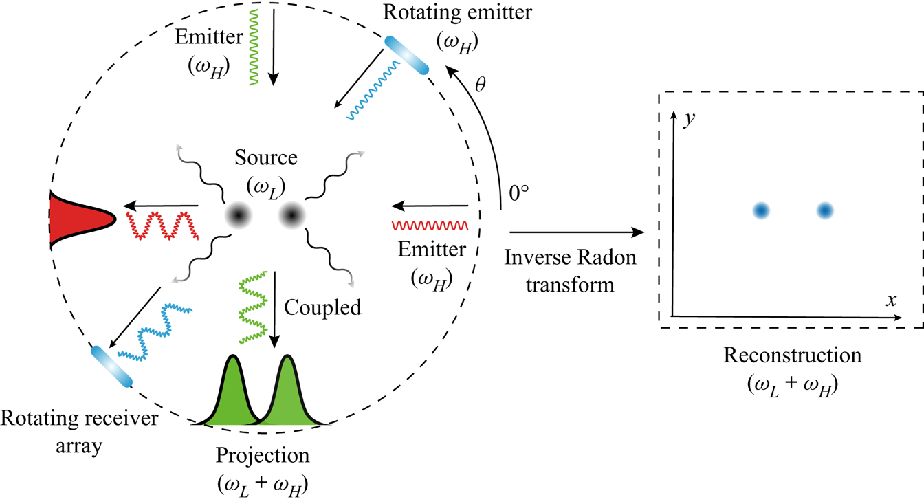
Figure 1 illustrates the key steps of the proposed method. First, high-frequency incident waves at angular frequency $\omega _H$ are introduced from various directions towards the target sound sources. In practical applications, the plane wave can be synthesised by employing an array of emitters, as shown in figure 1. Alternatively, a point source located at a far distance could also approximately yield a plane wave when the curvature of the wavefront is small and the amplitude is slowly varying. Here $\omega$ represents the angular frequency, and the subscript $(\cdot )_H$ denotes the high-frequency component. The low-frequency components are denoted by the subscript $(\cdot )_L$. Then, the incident waves will interact with the low-frequency target sound sources at $\omega _L$, which would produce new equivalent sources at $\omega _L+\omega _H$ due to the nonlinear effect (Westervelt Reference Westervelt1963; Beyer Reference Beyer1973). The acoustic signatures at $\omega _L+\omega _H$ are then recorded by an array of receivers placed in the opposite direction (to the emitters).

Figure 1.

Conceptual illustration of the extended-resolution imaging method for low-frequency sources at $\omega _L$. The emitters (to produce high-frequency plane waves at $\omega _H$) and receivers (to record the induced waves at $\omega _L+\omega _H$) are placed at different angles $\theta$. The acoustic image is reconstructed by performing the inverse Radon transform using data from the receivers.

The detailed mathematical formulations are given in § 3. Notably, the particular discussions therein for the induced nonlinear sound sources modelled from the flow governing equations are to some extent similar to those in the parametric acoustic array (Westervelt Reference Westervelt1963). However, the two methods are actually very different. The acoustic parametric array is often employed to generate acoustic beams with desired directivity patterns for sonar applications or inverse detection of medium properties. In contrast, the current study focuses on the extended-resolution imaging of low-frequency sources to account for the testing needs in aeroacoustic applications.

Physically, the induced sound signals perceived by the receivers can be regarded as the projection of the low-frequency target source at $\omega _L$ being swept by the external high-frequency plane wave at $\omega _H$. In practice, the distribution of low-frequency sound sources could be arbitrary (and unknown), and the projections of different sound sources swept by a single plane wave could be overlapped at the receivers. For example, as shown in figure 1, the two sources located at the $x_1$-axis being subjected to the incident wave at the incident angle $\theta =0^\circ$ can yield a single overlapped projection (which is presented in red in the figure). In contrast, for a plane wave at an alternative incident angle of $\theta =90^\circ$, the source locations can be identified as illustrated by the green peaks shown in figure 1. To this end, the external plane waves should be introduced from various directions, with incident angle $\theta$ ranging from $0^\circ$ to $360^\circ$, for practical applications, as the source locations are unknown a priori. Therefore, we need to rotate the emitter and receiver arrays for source imaging (as illustrated by the blue elements in figure 1). However, when necessary, we can also employ fixed emitters and receivers (since they are always in opposite directions), and rotationally adjust the target sources to achieve equivalent and varying incident angles $\theta$.

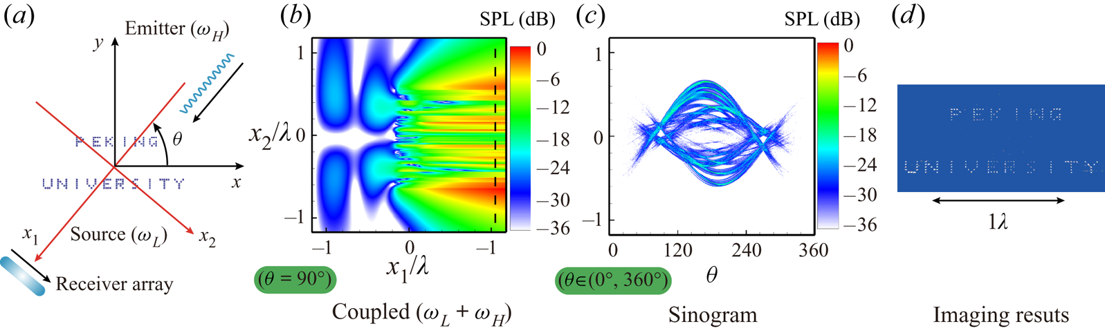
Figure 2 demonstrates the procedures of the proposed methods for extended-resolution source imaging, where $155$ point sources that construct the words ‘PEKING UNIVERSITY’ are studied. The frequency of the sources is $f_L=200$ Hz, and the phases are randomly different. The corresponding wavelength is $\lambda =7.4$ m (in water). The smallest separation distance within the source is $d=0.2~\mathrm {m}\approx 0.027\lambda$, which is far beyond the resolution capability of existing acoustic imaging methods. For this case, we employ incident plane waves at $f_H=120$ kHz from varying directions, as shown in figure 2(a).

Figure 2.

Illustration of the implementation procedure for the proposed extended-resolution imaging method. (a) High-frequency plane waves at $f_H$ are incident onto the point sources at a low frequency $f_L$. (b) The sound pressure distribution at the frequency of $f_L+f_H$ in $(x_1,x_2)$ coordinates when the incident angle is $\theta =90^\circ$. The black dashed line indicates the locations of the receivers. (c) Sinogram of the sound pressure recorded at the receivers for incident plane waves at various $\theta$. (d) The reconstructed sound source distributions.

Without loss of generality, the acoustic signals are recorded in the two-dimensional (2-D) domain for post-processing. Owing to the nonlinear interaction, additional acoustic components at frequency $f=f_L+f_H$ are produced and extracted by performing a Fourier transform on the recorded temporal sound pressure signals. As an example, the distribution of the induced sound component due to the nonlinearity for $\theta =90^\circ$ is shown in figure 2(b). The recorded sound component is directly linked to the low-frequency sources. For this demonstration case, the sound pressure is computed by the equivalent source $S_C=\rho _0\partial ^2(u_i^Lu_j^H)/\partial x_i\partial x_j$, where $u_i^L$ and $u_j^H$ are the acoustic particle velocities of the low-frequency sources and high-frequency plane waves, respectively. The details of the theoretical derivation are given in § 3. In particular, the sound pressure at the receivers, as indicated by the black dashed line in figure 2(b), is recorded. As given in the following analysis, when $\theta =0^\circ$, the recorded sound pressure at the observer/receiver $(x_1,x_2)$ can be approximately computed as

(2.1)\begin{equation} p(x_1,x_2,t) \approx \textrm{i}\rho_0A_Hk_H\exp(\textrm{i}\omega t - \textrm{i}k x_1) \int_{-\infty}^{x_1}u_1^L(\xi_1,x_2)\exp(\textrm{i}k_L\xi)\,\mathrm{d}\xi_1, \end{equation}

where $\omega =2{\rm \pi} f=2{\rm \pi} f_L+2{\rm \pi} f_H = \omega _L+\omega _H$ is the angular frequency of the induced sound, $k_H=\omega _H/c_0$, $k_L=\omega _L/c_0$ and $k=k_H+k_L$ are the acoustic wavenumbers, $c_0$ is the speed of sound, $\rho _0$ is the density, $u_1^L$ is the acoustic particle velocity of the low-frequency sound in the $x_1$-direction, and $A_H$ is the amplitude of the incident plane wave. It is worthwhile to mention that the rotating coordinates $(x_1, x_2)$ are shown in figure 2(a) with respect to the stationary coordinates $(x, y)$. The term $\exp (\textrm {i}\omega t - \textrm {i}k x_1)$ in (2.1) represents the dispersion relation of the induced sound at $f=f_L+f_H$. At the same time, the integral part suggests that the recorded sound at the receivers is the spatially accumulated projection of the low-frequency sound sources swept by the plane wave.

The integral in (2.1) represents a Fourier transform that would select the proper wavenumber component, i.e. the integral is non-zero if and only if the integration path $\xi _1\in (-\infty ,x_1)$ goes across any source location at $(\xi _1, x_2)$. Therefore, the relative locations in the $x_2$-direction are identified. To obtain the complete information of the sources in the whole space, the same procedure is performed in various directions, corresponding to the Fourier transform along different integration paths. When $\theta$ ranges from $0^\circ$ to $360^\circ$, the distribution of the sound pressures on the receivers at various transverse locations, as indicated by the black dashed line in figure 2(b), can be obtained. The pressure distribution on the $\theta$–$x_2$ domain is referred to as a sinogram, as shown in figure 2(c) for this guiding example. Finally, by performing the inverse Radon transform (Wu & Toksöz Reference Wu and Toksöz1987; Natterer Reference Natterer2001) on the sinogram, the original low-frequency sound sources can be reconstructed, and the result is shown in figure 2(d).

It should be mentioned that figure 2 demonstrates the procedures where the incident plane waves and the receiver arrays are simultaneously rotated. Mathematically, there would be little difference when the sources are rotated (while the emitters and receivers are fixed). Such a change of coordinate system would not have any influence on the final results. Moreover, to acquire the sound field in the whole field (see figure 2b) is expensive and unnecessary in practical experiments, and can therefore be omitted. Hence, we only need to acquire the data at the receivers to produce the sinogram.

3. Acoustic analogy-based tomography

In this section, details of the theoretical background of the proposed testing method, including the physics of the nonlinear coupling, the link between the low-frequency and induced equivalent sources, the solutions of the extended-resolution imaging and the associated mathematical techniques, are given. The derivations are based on the acoustic analogy along with the Born approximation. The same theoretical manipulations were adopted in our former study (Huang, Zhong & Liu Reference Huang, Zhong and Liu2014). Readers who are interested only in the proposed testing method can directly jump to the numerical and experimental demonstrations in the following sections.

3.1. Equivalent acoustic sources

First, we explain the wave model. The derivation starts from the inviscid fluid governing equations that allow for the direct study of the sound generation and propagation with the nonlinearity considered. By neglecting viscosity effects, we use the Euler equations, which consist of the following time-dependent continuity and momentum equations:

(3.1)\begin{gather} \frac{\partial\mathcal{R}}{\partial t} + {\frac{\partial(\mathcal{R} U_i)}{\partial x_i} }= 0, \end{gather}

(3.2)\begin{gather} \frac{\partial(\mathcal{R} U_i)}{\partial t} + {\frac{\partial(\mathcal{R} U_iU_j)}{\partial x_j} }+ \frac{\partial P}{\partial x_i} = 0, \end{gather}

where $\mathcal {R}$, $\boldsymbol {U}$ and $P$ are flow density, velocity and pressure, respectively. Following the standard practice in deriving the wave equation, we apply $\partial /\partial t$ and $\partial /\partial x_i$ to (3.1) and (3.2), respectively, and subtract the resultant equations, resulting in

(3.3)\begin{equation} \frac{\partial^2\mathcal{R}}{\partial t^2} - \frac{\partial^2P}{\partial x_i^2} = {\frac{\partial^2(\mathcal{R} U_iU_j)}{\partial x_i\partial x_j}}. \end{equation}

The procedures are substantially similar to the acoustic analogy that recasts the flow governing equations to an inhomogeneous wave equation (Lighthill Reference Lighthill1952).

Next, we decompose the flow variables into the uniform mean components denoted by $(\cdot )_0$ and the fluctuation components

\[ P = p_0 + p, \quad\mathcal{R}=\rho_0 + \rho, \quad U_{i} = U_{i_0}+u_{i}. \]

For practical applications, there could be some background mean flow, which could (1) produce aerodynamic noise that needs to be identified, and (2) influence the sound propagation and radiation. Both are challenging, and the related detailed discussion of the physics problem may distract our focus here, which is primarily on the development of a new method. To this end, as an early stage in our series of research, for simplicity, we assume that the background medium is stationary such that $U_{i_0}\equiv 0$ and $p_0$ and $\rho _0$ are uniform. For isentropic fluids, the pressure fluctuation and density fluctuation satisfy the relation $p=\rho c_0^2$, where $c_0$ is the speed of sound for the background fluid medium. Then, we rewrite (3.3) as an inhomogeneous wave equation in terms of the pressure fluctuation $p$:

(3.4)\begin{equation} \frac{1}{c_0^2}\frac{\partial^2p}{\partial t^2} - \frac{\partial^2p}{\partial x_i\partial x_i} = {\frac{\partial^2(\rho_0 u_iu_j+\rho u_iu_j)}{\partial x_i\partial x_j}. } \end{equation}

Here, the term on the right-hand side is the equivalent acoustic source, which is represented by $S(\boldsymbol {x}, t)$ in the remaining text, where $\boldsymbol {x} = (x_1, x_2)$. Physically, (3.4) suggests that sound waves are produced due to the spatial distribution and coupling of the fluctuations.

3.2. The Born approximation

Next, we explain the appearance of the equivalent sources when external high-frequency waves are incident on low-frequency acoustic sources. Equation (3.4) is exactly derived from the flow governing equations. However, it is difficult to solve that equation, as the equivalent source $S(\boldsymbol {x}, t)$ contains unknown variables such as $u_i$ and $\rho$. Under the small-amplitude assumption of the fluctuation variables, we can omit $\rho u_iu_j$ since they are of the third order of the fluctuations while $\rho _0 u_iu_j$ are of the second order. Then, the remaining part in $S(\boldsymbol {x},t)$ is evaluated by the Born approximation (Huang etal. Reference Huang, Zhong and Liu2014).

The particle velocities of the low-frequency and high-frequency sound waves are denoted as $u_{i,j}^L(\boldsymbol {x}, t)= u_{i,j}^L(\boldsymbol {x})\exp (\textrm {i}\omega _{L}t)$ and $u_{i,j}^H(\boldsymbol {x},\boldsymbol {t})=u_{i,j}^H(\boldsymbol {x})\exp (\textrm {i}\omega _{H}t)$, respectively. Usually, the interaction between the two sound components can induce new sound components that will contribute to velocity fluctuation. However, we further assume that the corresponding source is of low amplitude such that the velocity fluctuation in $S(\boldsymbol {x},t)$ is approximately computed as $u_{i,j}(\boldsymbol {x}, t)=u_{i,j}^L(\boldsymbol {x}, t) + u_{i,j}^H(\boldsymbol {x}, t)$. Then the equivalent source $S(\boldsymbol {x},t)$ is evaluated as

(3.5)\begin{align} S(\boldsymbol{x}, t) & \approx \frac{\partial^2}{\partial x_i\partial x_j} \left[\rho_0(u_{i}^L(\boldsymbol{x}) \exp({\textrm{i}\omega_{L}t}) + u_{i}^H(\boldsymbol{x})\exp({\textrm{i}\omega_{H}t}))\right.\nonumber\\ &\quad \left.\times(u_{j}^L(\boldsymbol{x}) \exp({\textrm{i}\omega_{L}t}) + u_{j}^H(\boldsymbol{x}) \exp({\textrm{i}\omega_{H}t}))\right]\nonumber\\ &= \underbrace{S_{L}(\boldsymbol{x})\exp({2\textrm{i}\omega_{L}t})}_{S_L(\boldsymbol{x}, t)}+ \underbrace{S_{H}(\boldsymbol{x})\exp({2\textrm{i}\omega_{H}t})}_{S_H(\boldsymbol{x}, t)}+ \underbrace{S_C(\boldsymbol{x})\exp({\textrm{i}(\omega_{L}+\omega_{H})t})}_{S_C(\boldsymbol{x}, t)}, \end{align}

which clearly shows that new wave components at frequencies other than $\omega _L$ and $\omega _H$ would appear due to the nonlinear coupling and interaction. The three terms are denoted as $S_L$, $S_H$ and $S_C$, depending on the corresponding (angular) frequency.

For the low-frequency source $S_L$, the associated angular frequency $2\omega _{L}$ is still so small that it would prevent high-resolution imaging operations. For the high-frequency source $S_H$ at the angular frequency $2\omega _H$, the associated amplitude $S_{H}(\boldsymbol {x})$ does not contain any information about the sound components at $\omega _L$, from which it would be impossible to reconstruct the target sources at $\omega _L$. For the interaction term $S_C$, the angular frequency is $\omega =\omega _{L}+\omega _H\gg \omega _L$, and the amplitude can be calculated as

(3.6)\begin{equation} S_C(\boldsymbol{x}, t) = 2 {\frac{\partial^2(\rho_0u_{i}^Lu_{j}^H)}{\partial x_i\partial x_j}}, \end{equation}

which contains information about the low-frequency target sound at $\omega _L$. Also, $\omega =\omega _L+\omega _H$ could be sufficiently high to yield satisfactory imaging resolution when $\omega _{H} \gg \omega _L$. Hence, we will focus on the coupled components $S_C$ at the angular frequency of $\omega$.

The propagation of the corresponding sound pressure is governed by the following inhomogeneous wave equation:

(3.7)\begin{equation} \frac{1}{c_0^2}\frac{\partial^2p}{\partial t^2} - \frac{\partial^2p}{\partial x_i^2} = S_C(\boldsymbol{x})\exp({\textrm{i} {(}\omega_{L}+\omega_{H} {)}t}). \end{equation}

Once the equation is solved, the induced particle velocity can be obtained. We may also solve the inhomogeneous wave equations using $S_L$ and $S_H$, respectively, to compute the induced velocity at other frequencies. Those induced fluctuations can then be added to $u_i^L+u_i^L$ to update the evaluation of $u_i$, leading to the higher-order Born approximations (He, Zhong & Huang Reference He, Zhong and Huang2019). However, the process will become convoluted and is undesirable for practical application. Moreover, the coupling between those components can only yield induced sound at different frequencies other than $\omega =\omega _L+\omega _H$. Therefore, by performing the Fourier transform, we can filter out those components such that the analysis to reconstruct the low-frequency sound from $S_C$ (at $\omega$) is not influenced.

3.3. Solution of the induced sound

Next, we explicitly (and approximately) compute the induced sound at $\omega =\omega _L+\omega _H$. Without loss of generality, we assume that the external high-frequency plane wave only propagates along the $x_1$-axis (i.e. the incident angle is $\theta =0^\circ$) in the 2-D domain:

(3.8a,b)\begin{equation} {u}^H_1(\boldsymbol{x},t) = A_{H} \exp({\textrm{i}\omega_{H}t-\textrm{i}k_{H}x_1}), \quad {u}^H_2(\boldsymbol{x},t) =0, \end{equation}

where $A_H$ is the amplitude and $k_{H}={\omega _{H}}/{c_0}$ is the acoustic wavenumber of the high-frequency component. Also, we represent the particle velocities of the low-frequency sound waves in both the $x_1$- and $x_2$-directions as

(3.9)\begin{equation} {u}_{1,2}^{L}(\boldsymbol{x},t)={u}_{1,2}^{L}(\boldsymbol{x})\exp({\textrm{i}\omega_{L}t}). \end{equation}

Substituting (3.8a,b) and (3.9) into (3.6), we obtain the representation of the equivalent source $S_C$ as

(3.10)\begin{equation} S_C(\boldsymbol{x},t)= 2\rho_0A_{H}\frac{\partial^2}{\partial x_1\partial x_j} \underbrace{\left[{u}_j^L(\boldsymbol{x})\exp({-\textrm{i}k_{H}x_1})\right]}_{{g}(\boldsymbol{x})} \exp({\textrm{i}\omega t}), \end{equation}

where $\omega =\omega _H + \omega _L$.

The function ${g}(\boldsymbol {x})$ defined in (3.10) consists of a rapidly oscillating component $\exp ({-\textrm {i}k_{H}x_1})$ and a slowly varying component ${u}^L_j(\boldsymbol {x})$. As a result, the spatial derivative of ${g}(\boldsymbol {x})$ is dominated by the rapidly changing part, leading to

(3.11)\begin{align} S_C(\boldsymbol{x},t)&=-2\rho_0A_{H}k_{H}^2\exp({\textrm{i}\omega_{H}t-\textrm{i}k_{H}x_1}) {u}_1^L(\boldsymbol{x})\exp({\textrm{i}\omega_{L}t}) (1+\mathscr{E}_1)\nonumber\\ &\approx -2\rho_0A_{H}k_{H}^2\exp({\textrm{i}\omega_{H}t-\textrm{i}k_{H}x_1}) {{u}_1^L(\boldsymbol{x})\exp({\textrm{i}\omega_{L}t} )}. \end{align}

Here $\mathscr {E}_1$ is the approximation error due to the omission of the derivatives of the low-frequency components, and it can be computed as

\[ \mathscr{E}_1=\frac{\textrm{i}}{u_1^L(\boldsymbol{x}) k_H}\left(2\frac{\partial u_1^L(\boldsymbol{x})}{\partial x_1}+\frac{\partial u_2^L(\boldsymbol{x})}{\partial x_2}\right) - \frac{1}{u_1^L(\boldsymbol{x}) k_H^2}\frac{\partial^2 u_i^L(\boldsymbol{x})}{\partial x_1 \partial x_i}. \]

Knowing that the acoustic particle velocities of the low-frequency sound $u_i^L$ vary in space at the rate of $\exp ({-\textrm {i}k_Lx_1})$ (because the angular frequency is $\omega _L$), it can be deduced that the approximation error $\mathscr {E}_1$ is estimated as

(3.12)\begin{equation} \mathscr{E}_1 \sim \frac{k_L}{k_H}\frac{u_i^L}{u_1^L} + \frac{k_L^2}{k_H^2}\frac{u_i^L}{u_1^L} = O(\epsilon), \end{equation}

where $\epsilon = k_L/k_H$ is a small quantity when $\omega _H\gg \omega _{L}$. In addition, the second- and higher-order terms, if there are any, of $\epsilon$ are omitted in $\mathscr {E}_1$.

The physical interpretation of (3.11) is that the coupled source $S_C$ is carried by the plane wave at $\omega _H$, while its amplitude varies slowly in space at a similar rate to the low-frequency sound $u_j^L$. As a result, (3.7) can be approximately written as

(3.13)\begin{align} \frac{1}{c_0^2}\frac{\partial^2p}{\partial t^2} - \frac{\partial^2p}{\partial x_1^2} &\approx -2\rho_0A_{H}k_{H}^2\exp({\textrm{i}\omega_{H}t-\textrm{i}k_{H}x_1}){{u}_1^L(\boldsymbol{x}) \exp({\textrm{i}\omega_{L}t})}\nonumber\\ &=-2\rho_0A_{H}k_{H}^2{{u}_1^L(\boldsymbol{x})\exp({\textrm{i}k_{L}x_1})}\exp({\textrm{i} \omega t {-}\textrm{ {i}} k x_1}), \end{align}

where $\omega =\omega _{H}+\omega _{L}$ and $k=\omega /c_0$. Also, the source terms have a time dependence of $\exp ({\textrm {i}\omega t})$, i.e. the sound field has an angular frequency $\omega$. Then we can denote the solution of $p(\boldsymbol {x},t)$ by the following prescribed form:

(3.14)\begin{equation} p(\boldsymbol{x},t) = \mathcal{P}(\boldsymbol{x})\exp({\textrm{i}\omega t - \textrm{i}k x_1}). \end{equation}

The exponential term $\exp (\textrm {i}\omega t- \textrm {i}kx_1)$ accounts for the dispersion relation of the induced sound.

It is easy to show that

(3.15a,b)\begin{equation} \frac{\partial^2p}{\partial t^2} = -\omega^2\mathcal{P}(\boldsymbol{x}) \exp({\textrm{i}\omega t - \textrm{i}kx_1}), \quad \frac{\partial^2p}{\partial x_1^2} = \left[\frac{\partial^2\mathcal{P}}{\partial x_1^2} - 2\textrm{i}k\frac{\partial\mathcal{P}}{\partial x_1} - k^2 \mathcal{P}\right] \exp({\textrm{i}\omega t - \textrm{i}kx_1}). \end{equation}

Then (3.13) can be written as

(3.16)\begin{equation} \frac{\partial^2\mathcal{P}}{\partial x_1^2} - 2\textrm{i}k \frac{\partial\mathcal{P}}{\partial x_1} \approx \underbrace{2\rho_0A_{H}k_{H}^2{u}_1^L(\boldsymbol{x})\exp({\textrm{i}k_{L}x_1})}_{h(\boldsymbol{x})}, \end{equation}

where the time derivative term $(1/c_0^2)(\partial ^2p/\partial t^2) = -(\omega ^2/c_0^2)p$ is cancelled by the term $k^2\mathcal {P}\exp (\textrm {i}\omega t - \textrm {i}kx_1)$ due to the spatial derivative. For simplicity, the source term on the right-hand side is denoted as $h(\boldsymbol {x})=2\rho _0A_{H}k_H^2{u}_1^L(\boldsymbol {x})\exp ({\textrm {i}k_{L}x_1})$, which is slowly varying because both $\exp (\textrm {i}k_Lx_1)$ and $u_1^L$ are related to the low-frequency sound. We can also deduce that the wavenumbers of $h(\boldsymbol {x})$ are close to $k_L$ such that

(3.17a,b)\begin{equation} \frac{\partial h(x_1)}{\partial x_1}\sim k_Lh(x_1)\quad \Rightarrow\quad\frac{\partial^nh(x_1)}{\partial x_1^n}\sim k_L^nh(x_1). \end{equation}

To solve the equation, we denote

\[ \mathcal{Q} = \frac{\partial\mathcal{P}}{\partial x_1}, \]

and then (3.16) is rewritten as

(3.18)\begin{equation} \frac{\partial\mathcal{Q}}{\partial x_1} - 2\textrm{i}k\mathcal{Q} \approx h(\boldsymbol{x}), \end{equation}

in which the omitted approximation error is $\mathscr {E}_1h(\boldsymbol {x}) = O(\epsilon ) h(\boldsymbol {x})$. Considering that we only study the differentials with respect to $x_1$, the partial derivative $\partial /\partial x_1$ can then be replaced by $\mathrm {d}/\mathrm {d}x_1$ in the following derivations. Next, (3.18) can be regarded as a first-order ordinary differential equation (ODE) with respect to $\mathcal {Q}$, and the solution can be easily obtained as

(3.19)\begin{equation} \mathcal{Q}(x_1,x_2) = \exp({2\textrm{i}kx_1})\int_{-\infty}^{x_1}h(\xi_1,x_2)\exp({-2\textrm{i}k\xi_1})\, \mathrm{d}\xi_1 = \exp({2\textrm{i}kx_1}) I_0(x_1), \end{equation}

where the second argument $x_2$ has vanished from $I_0$ for simplicity. In addition, $I_0$ can be deduced by introducing the following relation:

(3.20)\begin{align} I_n(x_1) &= \int_{-\infty}^{x_1}h^{(n)}(\xi_1)\exp({-2\textrm{i}k\xi_1})\,\mathrm{d}\xi_1 \nonumber\\ & = \frac{\textrm{i}}{2k}\int_{-\infty}^{x_1}\left\{ {\frac{\mathrm{d}}{\mathrm{d}\xi_1}[h^{(n)}(\xi_1)\exp({-2\textrm{i}k\xi_1})] }-h^{(n+1)}(\xi_1)\exp({-2\textrm{i}k\xi_1})\right\} \mathrm{d}\xi_1\nonumber\\ &=\frac{\textrm{i}}{2k}\left[h^{(n)}(\xi_1)\exp({-2\textrm{i}k\xi_1})\right]_{- \infty}^{x_1} - \frac{\textrm{i}}{2k}I_{n+1}(x_1), \end{align}

and $h^{(n)}(x_1) = \mathrm {d}^nh/\mathrm {d}x_1^n$ is the $n\textrm {th}$-order derivative with respective to $x_1$. Also, the low-frequency sound waves vanish in the far field. Then, the relation with $h^{(n)}(\xi _1=-\infty )=0$ can be employed such that

\[ \left[h^{(n)}(\xi_1)\exp({-2\textrm{i}k\xi_1})\right]_{-\infty}^{x_1} = h^{(n)}(x_1)\exp({-2\textrm{i}kx_1}). \]

Therefore, from the recursive relation in (3.20), $I_0$ can be computed as an infinite series:

(3.21)\begin{align} I_0(x_1) &=\frac{\textrm{i}}{2k}h(x_1)\exp({-2\textrm{i}kx_1} )- \frac{i}{2k}I_1 = \cdots \nonumber\\ &= \frac{\textrm{i}}{2k}h(x_1)\exp({-2\textrm{i}kx_1}) - \sum_{n=1}^{\infty}\left(\frac{\textrm{i}}{2k}\right)^{n+1}h^{(n)}(x_1) \exp({-2\textrm{i}kx_1}). \end{align}

Recalling that $h(x_1)$ is slowly varying, the spatial derivatives of $h(x_1)$ can be approximately estimated by using (3.17a,b). Next, we can use the relation $k_L/k = k_L/(k_L+k_H)=\epsilon /(1+\epsilon )=O(\epsilon )$. Then, we have

(3.22)\begin{equation} \sum_{n=1}^{\infty}\left(\frac{\textrm{i}}{2k}\right)^{n+1}h^{(n)}(x_1) \sim \frac{\textrm{i}}{2k}\sum_{n=1}^{\infty}\left(\frac{\textrm{i}k_L}{2k}\right)^{n}h(x_1) \approx \frac{\textrm{i}}{2k}\frac{\textrm{i}\epsilon}{2}\frac{h(x_1)}{1-\textrm{i}\epsilon/2} = \frac{- h(x_1)}{4k}O(\epsilon), \end{equation}

where we have employed $|\textrm {i}k_L/2k| \approx \epsilon /2 \ll 1$. By combining (3.19), (3.21) and (3.22), the solution for $\mathcal {Q}$ can be evaluated as

(3.23)\begin{equation} \mathcal{Q}(\boldsymbol{x}) = \exp({2\textrm{i}kx_1}) \left[\frac{\textrm{i}}{2k}h(x_1) - \frac{O(\epsilon)}{4k}h(x_1)\right]\exp({-2\textrm{i}kx_1}) = \frac{\textrm{i}h(x_1)}{2k} - \frac{h(x_1)}{4k}O(\epsilon). \end{equation}

Recalling that $h(\boldsymbol {x})=2\rho _0A_{H}k_H^2{u}_1^L(\boldsymbol {x})\exp ({\textrm {i}k_{L}x_1})$ and that $k_H^2/k = k_H^2/(k_L+k_H) \approx k_H(1-\epsilon )$, the first-order ODE for $\mathcal {P}$ is

(3.24)\begin{equation} \frac{\partial \mathcal{P}}{\partial x_1} =\mathcal{Q}(\boldsymbol{x})= \textrm{i}\rho_0A_Hk_Hu_1^{L}(\boldsymbol{x})\exp(\textrm{i}k_Lx_1)(1 + \mathscr{E}_2), \end{equation}

and the approximation error is

(3.25)\begin{equation} \mathscr{E}_2 =-\left(1-\frac{\textrm{i}}{2}\right)O(\epsilon)=O(\epsilon). \end{equation}

Comparing with the remaining term on the right-hand side of (3.24), $\mathscr {E}_2$ is negligibly small when $\epsilon =k_L/k_H\ll 1$. In this case, the solution for $\mathcal {P}$ can be obtained as

(3.26)\begin{equation} \mathcal{P}({x_1,x_2}) = \textrm{i}{k_{H}}\rho_0A_{H}\int_{-\infty}^{x_1}{u}_1^L(\xi_1,x_2) \exp({\textrm{i}k_L\xi_1}) \,\mathrm{d}\xi_1. \end{equation}

From (3.14), the coupled pressure $p$ at the angular frequency $\omega =\omega _{L}+\omega _{H}$ is

(3.27)\begin{equation} p(\boldsymbol{x},t) = \textrm{i}k_{H}\rho_0A_{H} \exp({\textrm{i}\omega t-\textrm{i}kx_1}) \int_{-\infty}^{x_1}{u}_1^L(\xi_1,x_2)\exp({\textrm{i}k_{L}\xi_1})\,\mathrm{d}\xi_1, \end{equation}

which is the final formulation that we would apply to theoretical studies, numerical approximations and experimental preparations. For plane waves incident from other directions $\theta$, a similar formulation can be obtained by using the new coordinate system $X_1=x_1\cos \theta +x_2\sin \theta$ and $X_2=-x_1\sin \theta +x_2\cos \theta$. It is worthwhile to mention that the above derivations are simply conducted for 2-D configurations, but the extension to three-dimensional space should be straightforward. We also wish to admit that the representation of the induced sound pressure is to some extent similar to the results of the parametric acoustic array (Westervelt Reference Westervelt1963), whose attention, nevertheless, was mainly focused on the generation of acoustic beams with desired directivity patterns.

For practical applications, sources are more often than not of multiple frequencies, e.g. $f_L$ and $f_L^*$. By following (3.27), the corresponding projections would have different frequencies, such as $f=f_L+f_H$ and $f^*=f_L^*+f_H$, which can be separately extracted by performing the Fourier transform. Moreover, another concern is that the frequency of the induced sound may, coincidentally, be the same as that of the other target source, e.g. $f_L+f_H = f_L^*$, leading to erroneous results. In practice, we can simply address this issue by setting the incident plane waves with much higher frequency than the frequencies of the target sources of interest.

4. Numerical demonstration

The guiding example in § 2 was prepared by using the equivalent source model given in § 3, where a couple of simplifications and assumptions have been adopted to enable the theoretical derivations. To further demonstrate the performance of the proposed imaging approach, here we conduct 2-D numerical simulations of the Euler equations that directly model the entire nonlinear processes. We believe that the numerical simulations would also justify the simplifications and assumptions that have been made in the theoretical model. In the simulations, the low-frequency target sound wave sources are introduced into the right-hand side of the Euler equations, as follows:

(4.1)\begin{equation} \left.\begin{array}{c@{}} \displaystyle\dfrac{\partial U_i}{\partial t} + U_i\dfrac{\partial U_j}{\partial x_i} +\dfrac{1}{\mathcal{R}}\dfrac{\partial P}{\partial x_i} = {0}, \\ \displaystyle\dfrac{\partial\mathcal{R}}{\partial t} + U_i\dfrac{\partial \mathcal{R}}{\partial x_i} + \mathcal{R}\dfrac{\partial U_i}{\partial x_i} = \sum_{n=1}^{N}A_n{\exp\left(-\dfrac{r^2_n}{b^2}\ln2\right)} \cos(\omega_Lt),\\ \displaystyle\dfrac{\partial P}{\partial t} + U_i\dfrac{\partial P}{\partial x_i} + \gamma P\dfrac{\partial U_i}{\partial x_i} = c_0^2 \sum_{n=1}^{N}A_n{\exp\left(-\dfrac{r^2_n}{b^2}\ln2\right)}\cos(\omega_Lt). \end{array}\right\} \end{equation}

Here $\gamma =1.4$ is the ratio of specific heats of the ideal gas; $\omega _L$ and $b$ are the angular frequency and half-bandwidth of the low-frequency point sources, respectively; $N$ is the number of low-frequency point sources; $r_n=((x-x_{n})^2+(y-y_n)^2)^{1/2}$ is the distance to the $n\textrm {th}$ point source located at $(x_n,y_n)$; and $A_n$ is the amplitude. The equations are solved using high-order finite difference schemes (Hu, Hussaini & Manthey Reference Hu, Hussaini and Manthey1996; Ashcroft & Zhang Reference Ashcroft and Zhang2003), and buffer zones (Richards etal. Reference Richards, Zhang, Chen and Nelson2004) are employed in the boundaries to achieve the non-reflecting boundary condition and to incorporate the high-frequency incident plane waves. In this work, the frequencies of the target point sources and external plane waves are $f_L=50$ Hz and $f_H=5$ kHz, corresponding to the low- and high-frequency wavelengths of $\lambda =6.8$ m and $\lambda _H=0.068$ m, respectively. The amplitude of the plane wave is 100 Pa and the amplitude of each point source is $A_n=0.1\rho _0/\omega _L$.

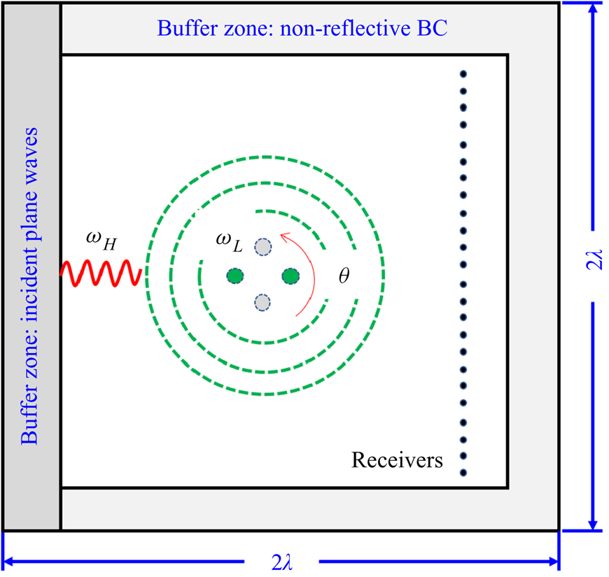
Figure 3 shows the schematic of the numerical simulations. For convenience, the locations of the inflow buffer zone (to introduce the high-frequency plane waves at $\omega _H$) and the receivers (to record the resultant induced sound pressure at $\omega _H+\omega _L$) are fixed, and the locations of the point sources are rotationally adjusted to yield the equivalent $\theta$. The numerical simulations are conducted in the 2-D domain with the dimensions of $2\lambda \times 2\lambda$, where $\lambda =c_0/f_L$ is the wavelength of the low-frequency sources. Because the current case set-up is rotationally symmetrical, the equivalent incident angle $\theta$ ranges from $-90^\circ$ to $90^\circ$ at an interval of ${\rm \Delta} \theta =2^\circ$, i.e. 91 cases are studied. The results at the remaining angles are obtained based on the symmetry of the problem.

Figure 3.

Schematic of the numerical simulations for the proposed extended-resolution acoustic imaging method. The plane waves are always introduced from the left boundary, and the source locations are rotationally adjusted to achieve the equivalent incident angles $\theta$.

A challenge in conducting the numerical simulations is that the wavelengths are significantly different for the high-frequency and low-frequency wave components. On the one hand, the dimensions of the computational domain should be large enough to allow the propagation of the low-frequency sound at $\omega _L$. On the other hand, sufficiently dense grids are required in the whole computational domain to avoid numerical dissipation for the high-frequency wave components. Currently, there are more than 12 grid points within a wavelength of the high-frequency sound $\lambda _H$. Consequently, the total grid number for this 2-D problem is approximately $8\times 10^7$. Also, the half-bandwidth for the point sources is $b=0.0474~\mathrm {m}\approx 0.7\lambda _H$, within which there are approximately nine grid points. In this work, we use the Alibaba Cloud supercomputing platform with 48 Xeon E5-2682 processors and 48 GB memory. For each simulation (at a given incident angle), it takes approximately 2.5 h to complete the calculation. The total $91$ cases can be conducted simultaneously, depending on the availability of computational resources. The sound pressures are recorded on $1200$ receivers as marked with black dots in figure 3. The sampling frequency is $f_s\approx 10f_H$, and the total sampling time is $0.5$ s, which equals 25 periods of the low-frequency sound. Once the data are collected, the reconstruction with our approach takes less than $5$ min to yield the acoustic images on an ordinary desktop computer.

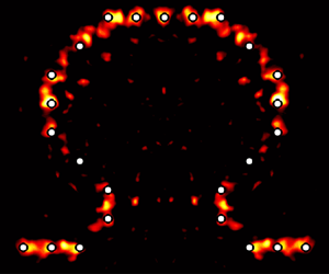
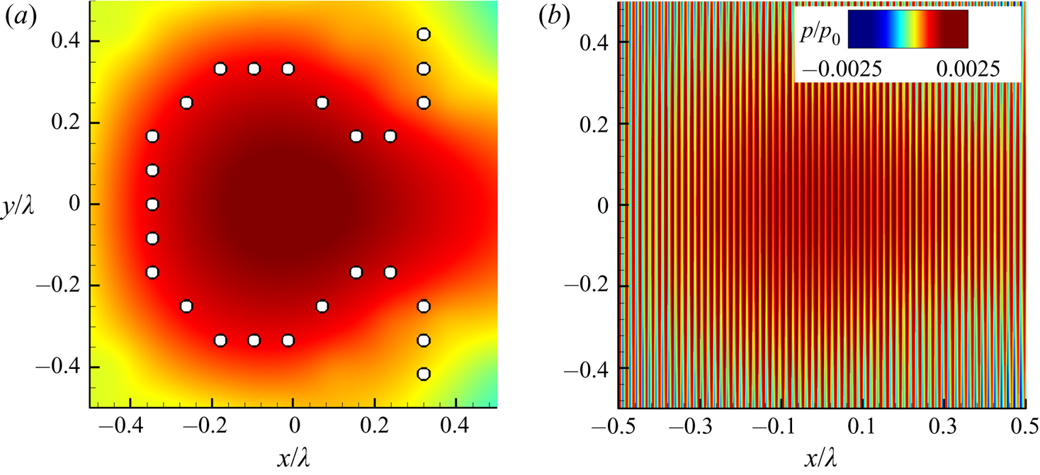
The demonstration case studies $25$ point sources that constitute the Greek letter ‘${\rm \Omega}$’, which represents a classical test set-up in imaging reconstructions. The smallest separation distance between the sources is almost $0.1\lambda$. The high-frequency plane waves have a frequency of 5 kHz. When the incident angle is $\theta =90^\circ$ (in the simulation the sources are rotated by $90^\circ$ equivalently), without introducing the plane wave, the locations of the sources along with the corresponding sound pressure distribution are shown in figure 4(a). Owing to the superposition of the point sources, it seems that the sound field has a maximum distribution in the centre of the computational domain. However, the sound field does not present any distinguishable structure of the source distribution since the distances are much smaller than the wavelength $\lambda$.

Figure 4.

Instantaneous sound distributions of the 25 low-frequency sources that form the letter ‘${\rm \Omega}$’. (a) Sound field produced by the low-frequency sources, which are indicated by the small circles. (b) Sound field of the total field with both low-frequency sources and high-frequency plane wave at the incident angle of $\theta =90^\circ$.

Next, figure 4(b) shows the instantaneous sound pressure distribution when the low-frequency sources are subjected to the incident plane wave at $\theta =90^\circ$.

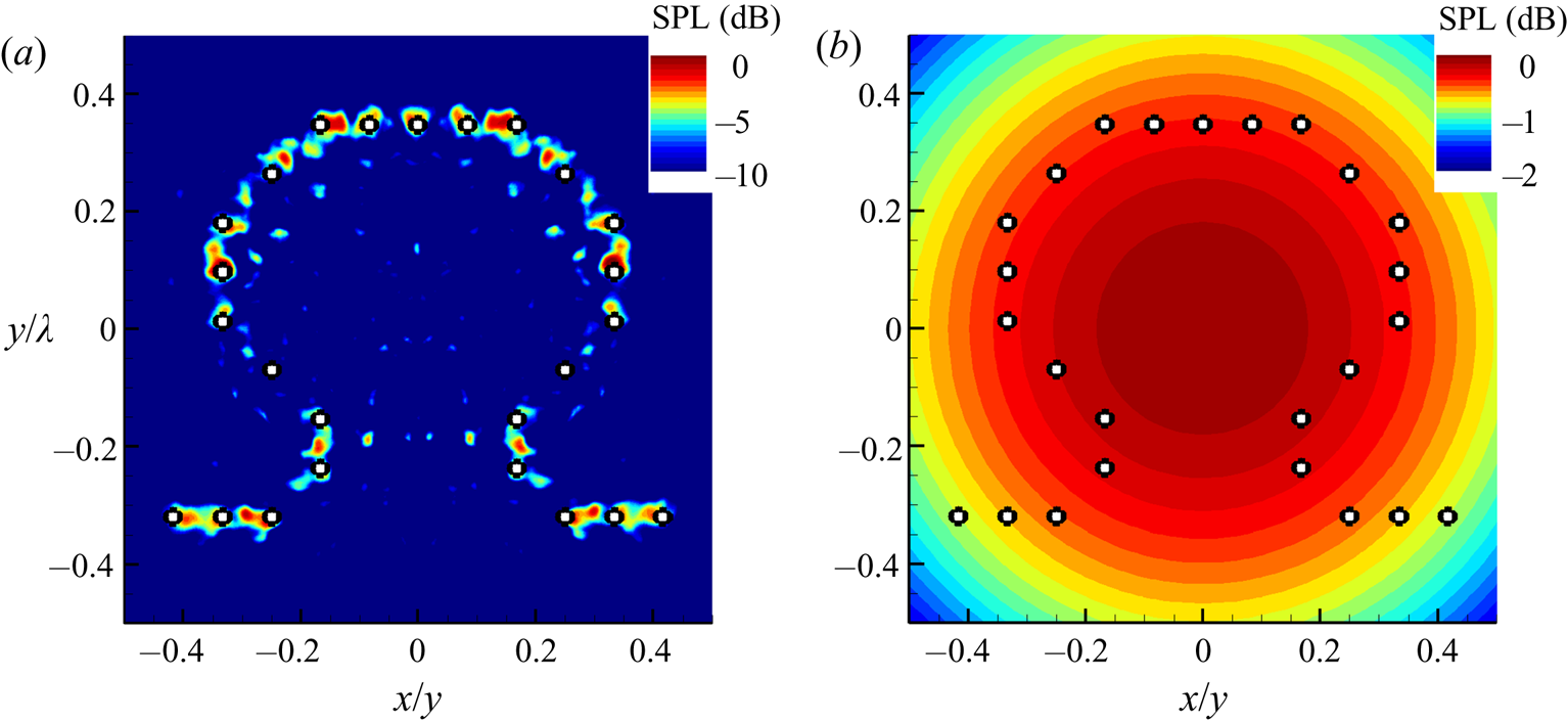
The acoustic imaging results based on the proposed method using the data collected from the $91$ computations are shown in figure 5. In general, figure 5(a) shows that both the locations and amplitudes of most point sources are reconstructed satisfactorily. Of course, it must be noted that some of the sources, such as the sixth one from the left, are not reconstructed completely, which is probably caused by the overlapping with our sources during the sweeping and/or numerical errors. The imaging performance could be further improved by reducing the interval of the incident angle ${\rm \Delta} \theta$ and by increasing $f_H$ (which is now $100f_L$) at a cost of extra computational resources. Nevertheless, the distribution of the ‘${\rm \Omega}$’ profile and the amplitudes are overall correct. In contrast, figure 5(b) shows the imaging result by the conventional beamforming, by which all point sources are completely indistinguishable.

Figure 5.

Acoustic images for 25 sources that form the Greek letter ${\rm \Omega}$ at 50 Hz using: (a) the proposed extended-resolution imaging method, and (b) the conventional beamforming method. The circles in each figure indicate the locations of the point sources.

Overall, from this numerical simulation case, we can conclude that the conventional method would be unable to help to reveal the associated physics when the frequency of interest is so low that it is beyond its imaging resolution, while our approach could be helpful because of the extended-resolution capability. Moreover, the reconstruction results based on direct simulations are consistent with those results based on the equivalent source model, which should help to justify those simplifications and assumptions adopted in the above theoretical developments in § 3.

5. Experimental demonstration

Next, we design and prepare experiments to demonstrate the performance of the proposed method. The experiment is conducted in a small, shallow water test rig established at Peking University. The speed of sound in the water is $c_0=1400$ m s$^{-1}$. The dimensions of the water tank are $0.8~\textrm {m} \times 1.1~\textrm {m} \times 0.1~\textrm {m}$. The boundaries of the rig are treated with pieces of acoustic rubber to minimise reflections. The size of each acoustic rubber piece is approximately $10~\textrm {cm} \times 10~\textrm {cm} \times 5~\textrm {cm}$. The width of the wedge is 1 cm and the height is $5$ cm. The amplitude of the reflecting wave is approximately 12 dB smaller than the calibration incident waves. 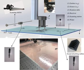The water depth is carefully controlled to be uniformly thin at $h=7$ mm, which enables us to assume a 2-D acoustic field inside the water. Figure 6 shows the whole experimental set-up.

Figure 6.

Experimental set-up for the proposed extend-resolution acoustic imaging method: (1) high-frequency emitters to generate plane waves at $f_H=120$ kHz; (2) two low-frequency acoustic sources at $f_L=200$ Hz with separation distance of $0.2$ m (approximately $0.027\lambda$); (3) rotation stage to hold and rotate the two acoustic sources; (4) array of receivers with aperture of $0.8$ m, with the distance to the two low-frequency sources being approximately $0.5$ m; (5) scanning station that holds the receivers; and (6) the shallow water tank.

We deploy the Brüel & Kjær 8103-type hydrophones in the water to produce high-frequency incident waves, as well as to measure the induced sound waves due to nonlinear coupling. In this work, we use a single hydrophone as emitter and the wavefront is circular. Nevertheless, with the increase of distance (from the hydrophone to low-frequency sources, approximately $0.6$ m in this work), the curvature of incident wavefronts becomes so small that this would approximate incident plane waves.

The low-frequency target sound waves are emitted from two off-the-shelf loudspeakers with a diameter of $d=18$ mm. In addition, the two loudspeakers are enclosed by bubble wraps, which are carefully controlled to be tangent to the water surface (rather than inserting into the water) to prevent the incident plane wave from being scattered from the two loudspeakers. The speakers have a flat frequency response between 100 Hz and 15 kHz. In this work, the loudspeakers are supported by a rotation stage such that the equivalent incident angle $\theta$ can be accurately adjusted. The main component of the rotation stage is the Daheng Optics table type GCM-1107M. In the experiments, the speakers are electrically driven by power amplifiers and signal generator at the lower frequency of 200 Hz. The corresponding wavelength in the water is 7 m. 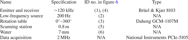Also, we deployed a screw rail to hold the receiver, which can be adjusted to different transverse locations ranging from $y=-0.4$ m to 0.4 m at an interval of 1 cm to record the sound signals consecutively. The equivalent aperture of the line sensor array is 0.8 m, which is still much smaller than the wavelength of the low-frequency sources and is, therefore, challenging for the conventional beamforming methods in acoustic imaging. The acoustic signals are acquired by using the National Instruments PCIe-5105. The sampling frequency is 2 MHz and the sampling time is 5 s. Table 1 gives detailed information about the main experimental components. In this work, the loudspeakers are not synchronised such that the sources are not in phase.

Table 1.

A summary of the experimental parameters.

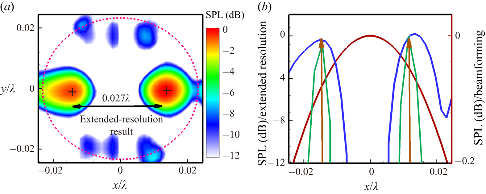
The sinogram is obtained with the data recorded on the receivers when the two point sources are rotated from $0^\circ$ to $360^\circ$ at an interval of ${\rm \Delta} \theta =22.5^\circ$. By performing an inverse Radon transform on the sinogram, we can reconstruct the acoustic image. As shown in figure 7(a), the proposed extended-solution approach identifies the two isolated sources well with a high dynamic range of 12 dB.

Figure 7.

Acoustic imaging results of the shallow water tank experiment. (a) Contour map result using the extended-resolution method. The beamforming results with the dynamic range of 0.1 dB is represented by the red dashed line. (b) Comparison of results along the $x$-axis. The two arrows are the actual source locations. The solid red curve represents the beamforming result, which does not identify the sources correctly. The solid blue curves and solid green lines are the results of the proposed method using the experimental and numerical data, respectively.

As a comparison, we also perform conventional beamforming using the same experimental data. The contour of the beamforming results is represented by the red dashed line in figure 7(a) with a very small dynamic range of only $0.1$ dB. In this case, with such a small dynamic range, the actual two point sources would still be incorrectly identified as a single one because the separation distance $0.027\lambda$ is too small to be distinguishable by conventional methods. We also wish to emphasise that post-processing type deconvolution methods (Brooks & Humphreys Reference Brooks and Humphreys2006) cannot resolve this issue.

Figure 7(b) compares the imaging performance of the acoustic imaging methods by quantifying imaging results on the line $y=0$. Again, by using the data collected in the experiments, only one lobe is found in the beamforming results with a meaningless dynamic range of 0.2 dB, i.e. the two sources are indistinguishable. In contrast, by using the proposed method, the locations and amplitudes of the two isolated point sources are correctly identified. We also conduct simulations for this case using the aforementioned numerical method in § 4, where the practical environmental uncertainties such as reflections and electromagnetic interference are completely absent. As a result, the associated imaging results should be improved, and figure 7(b) shows that the corresponding lobes in the source imaging are relatively narrowed.

6. Summary

In this work, we propose an extended-resolution imaging method for low-frequency sound sources. The procedures and performances are demonstrated using both numerical and experimental examples. The theoretical analysis based on acoustic analogy is conducted to explain the physical model, to simplify and solve the governing equations, and to clarify the difference between and connection to other methods/techniques. First, the nonlinearity of the sound waves is of crucial importance: the low-frequency sound sources (at $\omega _L$) are projected to a high-frequency counterpart (at $\omega _{L}+\omega _H$) by introducing external plane waves (at $\omega _{H}$) due to the nonlinear interactions. Then, the induced sound waves recorded at the receivers are decoupled and reconstructed by the inverse Radon transform to reconstruct the target sources. Essentially, the acoustic analogy and the Born approximation are incorporated into the tomography. We wish to emphasise that the popular term ‘super-resolution’ is deliberately avoided in this paper as the final imaging resolution is not superior to that of the high-frequency incident waves.

For the low-frequency sources of interest, the numerical and experimental results have demonstrated that the proposed technique can produce acoustic images with much higher resolution than the capability of conventional beamforming approaches. In this work, the low-frequency sources considered have a separation distance smaller than one-tenth to one-thirtieth of the corresponding wavelength, which is far beyond the resolution capability of the conventional beamforming methods. Moreover, the proposed method is theoretically straightforward and can be realised using relatively simple system designs. It shares similarities with the tomography technologies, so that the associated signal-processing methodologies and hardware are mature. Overall, the imaging technique could be a potential candidate for source imaging in acoustic and aeroacoustic applications, though much more effort is expected to tackle the practical issues. Future studies should consider the impacts of turbulent flows and solid boundaries (essentially by reformulating (3.7)), and consider to design and implement demonstrations that are more directly relevant to practical aeroacoustic applications.