Public opinion research is currently in the midst of several sweeping methodological transformations. For the better part of the past 60 years, most surveys have been based on probability samples, usually using the Mitofsky–Waksberg random digit dialing (RDD) procedure (Waksberg Reference Waksberg1978). Under RDD, calls are directed to randomly generated phone numbers within certain area codes and exchanges. For a time, this was an effective method in part because all residential landlines had some known (or plausibly estimated) positive probability of inclusion and because the target population was mostly reachable by landline.
In recent decades, however, the effectiveness of this method is being seriously questioned, forcing survey methodologists to come up with various ways to overcome its limitations. The need for improvements are especially pronounced, given several highly publicized polling “misses” in 2016: Brexit and the election of Donald Trump. Most public polls estimated a Remain victory in the UK. In the US, most national polls correctly estimated a victory for Hillary Clinton in the national popular vote, but state-specific polls were off—particularly in the “blue wall” states of Pennsylvania, Michigan, and Wisconsin—leading to a mistaken impression that Clinton would win the Electoral College and the Presidency.
Examples of recent innovations include cell phone supplements and internet polling. The prevalence of cell phones has made landline-only surveys inadequate, especially when trying to survey certain groups like young people or Hispanics. Cell phone supplements are increasingly recommended and used to combat this problem (AAPOR Cell Phone Task Force 2010). On top of this, response rates are in continual decline, increasing survey costs and placing the plausibility of weighting schemes that account for nonresponse into question. Many research firms are moving away from telephone surveys altogether as a result, and indeed away from probability sampling, preferring to use less expensive internet surveys (AAPOR Task Force 2013).
While these issues apply to surveys in general, political surveys present added sets of unique challenges. Registered or likely voters, as opposed to all adults, are often the target population. Likely voter screens—in which the interviewer asks one or a series of questions to determine whether a respondent is a likely voter and should continue with the survey—have been used for years, but they have many problems. First, the additional survey responses required to implement the screen make them costly. Second, the Gallup likely voter screen has been shown to bias its sample toward respondents who are excited by short-term political events, leading to exaggerated bounces and samples that are not easily comparable over time (Erikson, Panagopoulos, and Wlezien Reference Erikson, Panagopoulos and Wlezien2004). It is plausible that this happens when using likely voter screens outside of Gallup as well. Third, Rogers and Aida (Reference Rogers and Aida2011) used validated voting records to show that respondents are surprisingly bad at predicting whether or not they will vote, leading them to ask, “Why Bother Asking?”
Weighting or (post)stratification techniques mitigate some of these problems, but employing them properly is an additional challenge. The census is inappropriate for weighting toward likely or registered voter populations because it does not provide information on voting or registration. Alternatives exist, such as exit polls or the Current Population Survey’s (CPS) Voting and Registration Supplement, but they also have substantial problems. Exit polls have become increasingly problematic and difficult to implement (Barreto et al. Reference Barreto, Guerra, Marks, Nuño and Woods2006), and they are not available in every state or jurisdiction. And the CPS is itself a survey that relies on self-reported turnout and registration, leading to overreported estimates for these key measures. The extent of overreporting in the CPS is often misunderstood even by sophisticated researchers and practitioners due to a unique choice of how to code responses to the turnout question in the CPS (Hur and Achen Reference Hur and Achen2013).
Fortunately, new resources are available to help survey methodologists approach these serious challenges. Computational power is increasingly abundant and inexpensive, complemented by the explosion of newly available data sources. Together, these allow for smart and flexible statistical approaches to correct for some of these known biases and expand the inferential capabilities of survey analysts. For example, Ghitza and Gelman (Reference Ghitza and Gelman2013) show that multilevel regression and poststratification (MRP), in combination with census population estimates, could be used to construct survey estimates for demographic subgroups within states, estimates which cannot be plausibly estimated using standard techniques. When it comes to presidential forecasting, as another example, statistical approaches—such as those implemented on the popular websites fivethirtyeight.com and pollster.com—supplement traditional poll aggregation techniques to produce state-by-state preelection forecasts which were highly accurate in 2008 and 2012 but less accurate in 2016. Wang et al. (Reference Wang, Rothschild, Goel and Gelman2015) span both of these domains, using MRP to produce accurate state-level projections from highly nonrepresentative survey data collected from Microsoft’s Xbox gaming platform.
In this article, we are interested in one new data source in particular—national voter registration databases—and in how that data source can be used in conjunction with modern statistical techniques to improve the analysis of political surveys. These databases are a particularly attractive candidate for this purpose. Because the Secretary of State in each state is required by law to maintain a full list of registered voters, these databases enumerate the full target population of registered voters. Because they, again by law, keep track of who voted in every election,Footnote 1 they can be used to construct and enumerate a plausible likely voter population easily or to show the verified voter population after an election has taken place. Many states allow people to affiliate themselves with their desired political party at the time of registration, providing a stable record for perhaps the most important variable in structuring citizens’ political preferences (Campbell et al. Reference Campbell, Converse, Miller and Stokes1964). Finally, although these voter registration lists have been available to political scientists and survey methodologists in the past, only recently have they become easily accessible on a national scale, through private political vendors who collect, cleanse, standardize, and sell access to these databases to political campaigns, nonprofits, and academic institutions.
Other scholars have already documented certain ways these databases can be used. Green and Gerber (Reference Green and Gerber2006) tackle the problem of sampling a likely voter universe, arguing that registration-based sampling (RBS) allows for better stratification criteria due to the inclusion of auxiliary vote history variables. Rivers (Reference Rivers2007) uses large-scale databases in general, among which voter databases are a subset, to develop a sample-matching technique for web surveys. Rogers and Aida (Reference Rogers and Aida2011) show that records of past voting behavior from voter registration lists are substantially more accurate than self-prediction in forecasting future voter turnout behavior. McDonald (Reference McDonald2007) finds that the demographic distribution of the electorate on voter files matches expectations from election administration statistics and the CPS. Ansolabehere and Hersh (Reference Ansolabehere and Hersh2012) use voter databases to provide a valuable validation of multiple survey measures, such as turnout, registration, partisanship, and voting method. And these databases are increasingly used across a wide spectrum of political science research (Hersh and Schaffner Reference Hersh and Schaffner2013; Enos and Fowler Reference Enos and Fowler2014; Jackman and Spahn Reference Jackman and Spahn2015; Mann and Klofstad Reference Mann and Klofstad2015; Coppock and Green Reference Coppock and Green2016; Fraga Reference Fraga2016; Hersh and Nall Reference Hersh and Nall2016).
We extend MRP by applying it in combination with these new large-scale databases. In doing so, we propose a general method for survey analysis. The process proceeds by (1) either drawing a survey sample directly from the voter database or matching responses from an already existing survey to the database; (2) using auxiliary data from the database to construct a flexible statistical model on the quantity (or quantities) of interest; (3) projecting inferences from the statistical model to the full target population on an individual level; and (4) using the projected individual-level inferences, which can be seen as a pseudosurvey dataset, to construct larger group-level inferences about either the electorate as a whole or subgroups within the electorate.
We illustrate with an example, in which preelection polls from the 2012 presidential election are matched to a high-quality voter registration database and candidate preference estimates are produced for the full registered voter population. As we show through the article, these estimates, and the method in general, have a number of desirable properties. Our estimates appear stable and plausible to a high degree of geographic and subgroup specificity. They are similar to exit polls at both the national and state levels, and they can be used to drill down to much smaller geographies or subgroups than what is available from exit polls alone. It is easy to produce estimates for both the registered or verified voter populations. Finally, auxiliary information available in the voter databases allows for powerful and informative secondary analyses, beyond the standard inferences available from surveys alone.
At the same time, gains from using these new databases are not achieved without cost, and limitations and open problems remain. Our method requires expertise in both statistical modeling and the handling of “big data,” and the differences in data coverage across jurisdictions can lead to complications. Our example model is also built in a postelection context, and we frame it as a supplement to exit polls. In this postelection context, we leverage important information to improve our inferences (county-level election returns, turnout data). An obvious extension is in preelection polling and forecasting, where certain challenges remain. We discuss some of the open challenges in using our framework for survey analysis moving forward.
Although our approach is, in some sense, simply an application of an existing statistical method (MRP), this paper illustrates how better data and more computational resources can improve and deepen public opinion estimates obtained through MRP. We extend the “deep interactions” estimates of Ghitza and Gelman (Reference Ghitza and Gelman2013), increasing the breadth of the multilevel model from five factors to twelve.Footnote 2 Politically important covariates—such as party registration and past voting behavior—are available on the target population dataset, in contrast to the data available on the census, allowing us to incorporate them into the model and inferences.
We also take advantage of the scale of our data by making a conceptual move toward individual-level records. Ghitza and Gelman (Reference Ghitza and Gelman2013) produce inferences for subgroup-level population cells—African American women in Kansas, for example—which could be arbitrarily combined to provide poststratified estimates for larger groups. We build a model and score it on the database of over 190 million people, facilitating more flexible poststratification. Each individual-level population cell is, in reality, a group-level cell conditional on the 12 factors in the model, 15 additional continuous covariates, and the functional form of the model.
It is important to note that, although the use of these voter databases is still relatively rare in both academic political science and publicly available political polls, they have already become important tools within political campaigns and civic advocacy organizations. The methods presented here can be seen as falling within a family of techniques already used inside these organizations.Footnote 3 Still, our method is a substantial departure even in that context, for three reasons. First, the so-called “microtargeting models” in political campaigns have primarily been used to drive individual-level voter contact—they are used to rank the priority of contacting individuals on a person-by-person basis, as opposed to finding precise point estimates. Second, these models are generally applied toward individual-level political marketing, rarely (or inappropriately) in the context of finding group-level estimates, which is the driving motivation behind this paper. Third, this is the first time that measures of uncertainty are propagated through the full process. Though our method does not account for all of the uncertainty in the process (as described in Section 4), we account for and display estimates of sampling and modeling uncertainty through the full procedure.
The paper will proceed as follows. We describe the voter registration database, along with the surveys that have been matched to the database to facilitate the analysis. We then lay out our statistical and computational methods—the statistical model, variable specification, and computational details. Once these tasks are completed, we share our results, illustrating several examples of what can be done with our model-based inferences. We close with the discussion.
1 Data
We use data from a voter registration database to approximate 2012 presidential voting preferences (Ghitza and Gelman Reference Ghitza and Gelman2019). Our strategy is to use self-reported presidential voting preferences from a phone survey to build a statistical model predicting vote choice conditional on covariates from the database. To do this, we need two primary data sources—a national database of registered voters and a survey that is matched to that database.
Lists of registered voters are collected and maintained on a state-by-state basis, or in some states at a lower geographic level, by the Secretary of State. Scholars who have wanted to use this data in the past were often forced to collect this data directly from these local governments, with that data collection chore sometimes problematic due to the varying nature, cost, and quality of the data across jurisdictions. In this paper, we partnered with Catalist, LLC to use their national voter registration database. As Ansolabehere and Hersh (Reference Ansolabehere and Hersh2012) explain, Catalist collects, standardizes, and enhances the data available from the raw voter lists alone:
Catalist is a political data vendor that sells detailed registration and microtargeting data to the Democratic Party, unions, and left-of-center interest groups. Catalist and other similar businesses have created national voter registration files in the private market. They regularly collect voter registration data from all states and counties, clean the data, and make the records uniform. They then append hundreds of variables to each record. For example, using the registration addresses, they provide their clients with census information about the neighborhood in which each voter resides. Using name and address information, they contract with other commercial firms to append data on the consumer habits of each voter. (Ansolabehere and Hersh Reference Ansolabehere and Hersh2012, p. 441)
The work that goes into maintaining a high-quality dataset of this kind is quite complicated and detailed. Indeed, the quality of inferences drawn from this data is quite clearly dependent on the quality of the data in the database. Fortunately, Ansolabehere and Hersh provide a substantial amount of detail into Catalist’s matching methods, along with various forms of verification of Catalist’s data quality:
Three factors give us confidence that Catalist successfully links respondents to their voting record and thus provides a better understanding of the electorate than survey responses alone. These three factors are (1) an understanding of the data-cleansing procedure that precedes matching, which we learned about through over twenty hours of consultation time with Catalist’s staff; (2) two independent verifications of Catalist’s matching procedure, one by us and one by a third party that hosts an international competition for name-matching technologies; and (3) an investigation of the matched CCES, in which we find strong confirmatory evidence of successful matching. (Ansolabehere and Hersh Reference Ansolabehere and Hersh2012, p 442)
We pulled our data for this paper from Catalist at two points—just before the election, in November 2012, and after Catalist collected individual voter turnout records, in May 2013. By using data from both of these versions of the database, we were able to capture (1) people who were registered for the election but subsequently dropped off the file because they did not vote in 2012, and (2) new registrants who did not yet make it onto the voter rolls prior to the election.Footnote 4 Our target universe, then, comprises all people who had either an active or inactive voter registration status on either one of these two files, both of whom are eligible to vote in all states. Catalist also maintains records for people who have been dropped off the voter rolls as well as unregistered voting-aged people, but we do not consider them in this analysis. In total, our final target universe is 191,430,104 registered voters. Catalist’s full dataset is not generally available to scholars, but they do offer a 1% sample via a standard academic subscription as well as other data that can be purchased on a custom basis. In the Appendix, we show the similarity between estimates drawn from the full dataset and a 1% sample.
Our survey is collected from two sources. The first is a set of “tracking” surveys administered by Greenberg Quinlan Rosner Research (GQRR), a polling firm in Washington, DC. These surveys were pulled using RBS, with telephone numbers provided by Catalist. The RBS procedure produces a random sample of the registered voter population, conditional on the registered voter having a valid and recorded phone number. This will not, in general, produce a random sample of the full voting population due to some voters not having phone numbers and nonresponse. Here, we rely on the MRP procedure to correct for these biases, conditional on the covariates accounted for in the model. The second is a set of surveys collected for Democracy Corps, an independent nonprofit research organization. It uses RDD prescreened by Survey Sampling International for households with valid landline phones. This produces a random sample of the landline population, conditional on nonresponse, and again we will rely on MRP to produce estimates for the voting population. These survey responses were matched to the Catalist dataset using name, address, gender, birth year, and phone number in order to append the voter file covariates that we use for MRP. The matching procedure introduces some uncertainty into our procedure, in that a small percentage of survey respondents will be mismatched—that is, incorrect covariates will be appended to a survey response because the matching system incorrectly assigns the respondent to an incorrect database record, perhaps somebody with the same name and birth year but a different birth day.Footnote 5 Both types of surveys were conducted by GQRR and were provided by the AFL–CIO for this research. The data includes respondents from all 50 states and the District of Columbia, with data collection stratified by region and both sets of surveys including a cell phone supplement. All calls were conducted from the same call center, with the same supervising staff and training procedures. In total, these surveys sum to 17,424 respondents who expressed a preference for either Pres. Obama or Gov. Romney, collected from March 1 up to (but not including) Election Day, November 6, 2012.
2 Methods
2.1 Statistical Model
We model vote choice in the 2012 presidential election. The
 $n$
survey respondents are indexed using
 $i=1,\ldots ,n$
.
 $y_{i}$
indicates stated presidential support, with
 $y_{i}=1$
for the Democratic incumbent Barack Obama and
 $y_{i}=0$
for the Republican challenger Mitt Romney. Assuming that the survey respondents are independently and identically sampled, the data model is
 $y_{i}\sim \text{Bernoulli}(\unicode[STIX]{x1D703}_{i})$
, where
 $\unicode[STIX]{x1D703}_{i}$
is the probability of Obama support.
Our model is thus a logistic regression, which we will fit using a multilevel model. The response variable
 $y$
comes from the survey, but all of the input variables come from Catalist’s database. This is the key decision that allows us to project our inferences to the full target population—because all of the input variables are available for the full population through Catalist’s database, our resulting regression equation can be trivially used to project
 $\unicode[STIX]{x1D703}_{1}\ldots \unicode[STIX]{x1D703}_{N}$
onto the full
 $N$
members of the database.
We will build up our model in stages. It is convenient to split
 $\unicode[STIX]{x1D703}$
into two parts. The first represents varying intercepts for different discrete factors in the model and the second captures slopes for input variables that are not easily characterized as factors.
Varying intercepts. For concreteness, the population has
 $K$
factors, indexed as
 $j_{1}=\{1,\ldots ,J_{1}\}$
;
 $j_{2}=\{1,\ldots ,J_{2}\};\ldots ;\,j_{k}=\{1,\ldots ,J_{K}\}$
. These factors are variables in the database—such as gender, race, party registration, or state of residence—all of which can be split up into discrete levels; the number of levels for each
 $k$
factor is indexed using
 $J_{k}$
. The association between each of these variables and
 $y$
can be captured through a series of varying intercepts. The varying intercepts for factor
 $K$
are denoted as
 $\unicode[STIX]{x1D6FC}_{1}^{k}\ldots \unicode[STIX]{x1D6FC}_{J_{k}}^{k}$
, and so the resulting nonnested (crossed) equation is
 $$\begin{eqnarray}\displaystyle \unicode[STIX]{x1D703}_{i}=\text{logit}^{-1}\left(\displaystyle \mathop{\sum }_{k=1}^{K}\unicode[STIX]{x1D6FC}_{j_{k[i]}}^{k}\right). & & \displaystyle\end{eqnarray}$$
This model can be interpreted as a multilevel version of a logistic regression including “base” effects only. We would like to include two-way interactions between all of the factors as well. As such, there are
 $S$
total factors, including the set of all base factors plus two-way interactions, and
 $\unicode[STIX]{x1D6FC}^{s}$
replaces
 $\unicode[STIX]{x1D6FC}^{k}$
as our set of varying intercepts:
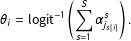 $$\begin{eqnarray}\displaystyle \unicode[STIX]{x1D703}_{i}=\text{logit}^{-1}\left(\displaystyle \mathop{\sum }_{s=1}^{S}\unicode[STIX]{x1D6FC}_{j_{s[i]}}^{s}\right). & & \displaystyle\end{eqnarray}$$
As an illustration, say our model only has
 $K=3$
base factors—sex (male; female), race (white; black; Hispanic; other), and state (51 states including the District of Columbia). There are therefore
 $S=6$
total factors—the original three plus sex
 $\times$
race, sex
 $\times$
state, and race
 $\times$
state—and this would imply
 $A=2+4+51+2\times 4+2\times 51+4\times 51=269$
total varying intercepts. With even this small number of factors, it becomes clear that using a multilevel model, instead of trying to include all interaction terms in a classic logistic regression, is the preferred approach.
Some prior information is necessary for us to expect a reasonable output with this many parameters. We regularize by setting zero-centered normal priors on all of the intercepts—
 $\unicode[STIX]{x1D6FC}^{s}\sim \text{Normal}(0,\unicode[STIX]{x1D70E}_{s})$
—and allowing the scale parameters to be estimated from the data. In our model, we will end up with
 $S=75$
. We model the scale parameters as coming from a common half-
 $t$
distribution,
 $\unicode[STIX]{x1D70E}_{s}\sim t^{+}(0,8,\unicode[STIX]{x1D70E}_{0})$
, with a uniform hyperprior on
 $\unicode[STIX]{x1D70E}_{0}$
. We do not expect the particular functional form of the
 $t$
model to be crucial; we choose it because it regularizes the estimates of
 $\unicode[STIX]{x1D70E}_{s}$
while allowing them to vary to the extent this is suggested by the data.
Varying slopes. On top of the
 $K$
discrete factors, Catalist’s auxiliary data also includes variables that are best treated as continuous. A few examples are age and estimated household income, which are individual-level characteristics, as well as geographic attributes such as percent of a person’s geographic area that is African American, data that is collected at geographies as small as census block groups.
These continuous inputs can be easily represented as varying slopes in our model. Let
 $L$
denote the number of continuous variables, and let
 $X$
denote the standardized
 $n\times L$
matrix of these variables for our
 $n$
survey respondents. To speed up computation, we standardize the variables by subtracting the mean and dividing by two standard deviations (Gelman and Hill Reference Gelman and Hill2007).
 $\unicode[STIX]{x1D6FD}^{1}\ldots \unicode[STIX]{x1D6FD}^{L}$
then indicate the
 $L$
slopes, and each of these slopes could in theory vary by each of the
 $S$
factors. In this case, the slopes are indexed
 $\unicode[STIX]{x1D6FD}_{s}^{1}\ldots \unicode[STIX]{x1D6FD}_{s}^{L}$
, with sets of
 $\unicode[STIX]{x1D6FD}$
s for each factor
 $s$
. If we subscript column
 $l$
of matrix
 $X$
as
 $X_{l}$
, the final equation is written as
 $$\begin{eqnarray}\displaystyle \unicode[STIX]{x1D703}_{i}=\text{logit}^{-1}\left(\displaystyle \mathop{\sum }_{s=1}^{S}\unicode[STIX]{x1D6FC}_{j_{s[i]}}^{s}+\displaystyle \mathop{\sum }_{l=1}^{L}\displaystyle \mathop{\sum }_{s=1}^{S}X_{l}\unicode[STIX]{x1D6FD}_{s[i]}^{l}\right) & & \displaystyle\end{eqnarray}$$
with the
 $\unicode[STIX]{x1D6FD}$
s having identical regularizing prior as the
 $\unicode[STIX]{x1D6FC}$
s. In practice, we do not vary all of our slopes by all of our factors, as this would lead to too many parameters for our model to reliably estimate. But this last equation accurately reflects the generalized form of the model.
2.2 Input Variables
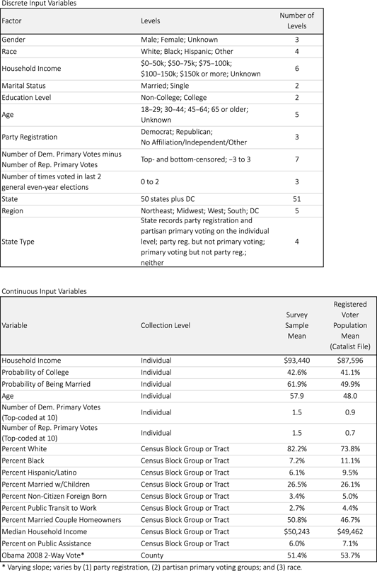
Ghitza and Gelman (Reference Ghitza and Gelman2013) fit a similar statistical model using up to five base factors and three continuous variables. Newly available software makes it easier to fit a larger statistical model, so our model is expanded considerably. Table 1 lists all of our variables. In the top panel, we have expanded from five factors to twelve. We include standard demographic variables—gender, race, household income, marital status, education level, and age.Footnote 6 Note that some of these variables include “Unknown” values. We keep these values as separate levels in the model. Consider gender as an example; some small percentage of values will be labeled as Unknown, in both the survey and the full poststratification database. We estimate vote choice for the Unknown group and project that onto the database and poststratified estimates themselves.
Variables from the Catalist database that are used as inputs into our statistical model. The twelve discrete variables include standard demographic and geographic factors, along with political variables such as party registration. Continuous variables are modeled as linear predictors, including individual-level data along with geographic variables collected at the census block group level or census tract level where that is not available. Differences between the survey sample and full registration database are easily apparent by looking at average values for these continuous variables.

We also include three political variables that are not available on the census and, indeed, are only available for any large population through voter databases such as the Catalist database. Most importantly, we use party registration, which is a close proxy for party identification, perhaps the dominant structural variable in American political behavior. By including this as a covariate, we gain a great deal of predictive power in our inferences. By using a person’s registration status as recorded on official records, we have the added benefit of eliminating the possibility of reverse causality or endogeneity that might exist if we used self-reported party ID and vote choice from within a single survey. Because registering with a certain political party is not allowed in some states, we use partisan primary voting as an additional strong indicator of partisan preferences. As noted earlier, voter registration databases keep records of past voting behavior—which elections were voted in, not which candidate was chosen. Some of those elections are partisan primaries, in which case voting in that election is a good indicator of partisanship and future voting preferences. Finally, we note each person’s level of political engagement, as reflected in how many times (s)he voted in the last two even-year general elections. Importantly, by interacting this with all of the other covariates in the model, we account for the relationship between each of those covariates and vote choice conditional on level of political engagement.
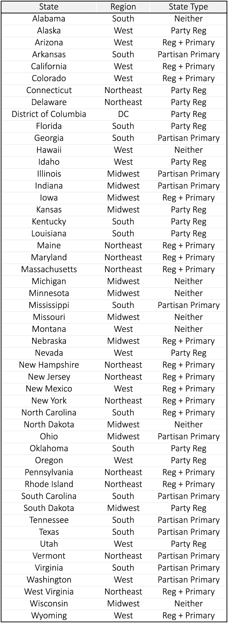
Definitions of state-level variables used in the MRP model.
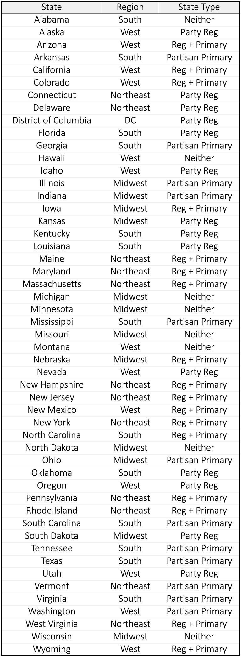
We also include state as a factor, as well as region and state type, both of which are defined on the state level and annotated in Table 2. By including state, again interacted with all of the other covariates, we allow for different effects in different states, if those differences are supported by the data. We partially pool within region to allow the model to pick up on regional trends in cases where there is not enough data to support state-specific trends. Finally, state type is used to distinguish different administrative levels of record-keeping across states. Some states allow for registering with a particular party, some states record partisan primary voting, and some states do both or neither. The four state types encompass these combinations and allow other covariates to have different levels of importance in different state types. For example, in states where most people are registered as Democrats or Republicans, we expect party registration to have a large effect and soak up much of the variance in the equation. But in states with a small number of party registrants, we would like other covariates, such as income and race, to be able to have a larger impact on our final estimates.
Next we move to our continuous input variables, all included as linear predictors. Note that some are individual-level variables which mirror variables that have also been included as discrete factors. In a classical regression setting, we would have to choose whether to include each variable as a single linear variable or as groups of indicator variables in order to avoid multicollinearity. One benefit of using the multilevel model here is that we can include these variables as both, allowing the model to pick up on strong linear effects through the continuous variable and also allowing for nonlinear or even nonmonotonic effects through the factors. We also include nine census geographic variables, defined at either the census block group level or, where that level of specificity is not available, at the tract level. Finally, we include county-level vote choice from the 2008 election as the last variable. Because of the importance of this variable in particular, we allow the slope to vary by party registration, partisan primary voting groups, and race.
We list the sample and population means for each of the continuous variables in Table 1 as well. This provides two benefits: first, the reader can get a sense of reasonable values; second, we can immediately see that the sample and the population of registered voters are quite different for some variables. The sample has notably higher income, is older, votes in more primary elections, and lives in areas that are generally whiter and less urban—note that the sample features less public transit to work, less on public assistance, and more married couples with homeowners. The poststratification method described here automatically adjusts estimates to account for these biases, conditional on the covariates included and the model specification.
2.3 Computation
We fit the hierarchical regression using Stan (Stan Development Team 2013) and R (R Core Team 2012), using the roughly 17,000 survey responses containing self-reported vote intent and the described covariates.Footnote 7 This is one layer of computational complexity: when we consider all of the varying intercepts and varying slopes, there are 2484 total coefficients to consider (along with eighty additional hyperparameters). They represent the varying intercepts for almost 7 million combinations of each of the discrete factors, along with slopes for all of the continuous variables detailed earlier. We also want to project measures of uncertainty along with point estimates, so we draw 100 samples of each parameter from the posterior distribution of the model.Footnote 8
We then project
 $\unicode[STIX]{x1D703}$
to the full database, creating a 191 million
 $\times$
100 matrix
 $M$
, with
 $M$
representing 100 posterior draws of our estimated
 $\unicode[STIX]{x1D703}$
for each registered voter. Because
 $M$
is so large, we need to use a database that can efficiently store and handle computations of this magnitude.Footnote
9
We use the Vertica Analytic Database 5.0 with a four-node cluster (Lamb et al.
Reference Lamb, Fuller, Varadarajan, Tran, Vandiver, Doshi and Bear2012). We are agnostic as to whether this particular database solution is the most efficient for this problem, allowing us to analyze our resulting inferences, in conjunction with the remaining auxiliary data from Catalist, relatively quickly and easily using generic SQL syntax. It facilitates a relatively painless interface with R, in which we use the RJDBC package (Urbanek Reference Urbanek2012) to interface with the database using Vertica’s generic JDBC driver.
2.4 Poststratification and Intercept Correction
Once we have our matrix
 $M$
, it is trivial to aggregate
 $\unicode[STIX]{x1D703}$
s to provide poststratified estimates for arbitrarily defined populations of interest. To provide a point estimate for Obama support for the entire registered voter population, we could simply compute the average
 $\unicode[STIX]{x1D703}$
over the entire matrix. We could also perform the same calculation for specific geographies (such as state, county, congressional district, or state legislative district), demographically defined subgroups, or combinations of the two. In fact, we are now able to compute poststratified estimates for any subgroup that can be defined using any of Catalist’s auxiliary data.
One last step is a county-level intercept correction. Using county-level election returns and Catalist’s vote history records, we correct each county’s final estimate, within each of our 100 sample draws, to reflect actual vote totals. Let
 $\unicode[STIX]{x1D709}_{c}$
indicate the number of Obama voters for each county (or county-equivalent)
 $c=1,\ldots ,3143$
and let
 $C$
denote the set of registered voters in county
 $c$
. We derive the adjusted Obama support estimate
 $\unicode[STIX]{x1D703}_{i}^{\ast }$
for each registered voter
 $i\in C$
as follows:
 $$\begin{eqnarray}\displaystyle \unicode[STIX]{x1D6FF}_{c} & = & \displaystyle \text{argmin}\left(\text{abs}\left(\unicode[STIX]{x1D709}_{c}-\displaystyle \mathop{\sum }_{i\in C}\text{logit}^{-1}(\text{logit}(\unicode[STIX]{x1D703}_{i})+\unicode[STIX]{x1D6FF})\right)\right)\end{eqnarray}$$
 $$\begin{eqnarray}\displaystyle \unicode[STIX]{x1D703}_{i}^{\ast } & = & \displaystyle \text{logit}^{-1}(\text{logit}(\unicode[STIX]{x1D703}_{i})+\unicode[STIX]{x1D6FF}_{c})\quad \forall i\in C,\end{eqnarray}$$
where abs() is the absolute value function and argmin() is a function that finds the
 $\unicode[STIX]{x1D6FF}$
that minimizes the expression. This process simply applies a constant logistic adjustment
 $\unicode[STIX]{x1D6FF}_{c}$
to each registered voter in county
 $c$
to make sure that the total number of estimated Obama voters is correct.
While design-based inferences are unbiased conditional on perfect random sampling of the population, our model-based poststratified inferences avoid systematic error conditional on the covariates included in the model and the functional form of the hierarchical regression, plus the just-described county intercept correction. Omission of predictors that are correlated with vote preference, after accounting for the modeled covariates, may cause bias. This is why we specified such a flexible statistical model earlier and one that included as many covariates as it did. It is, of course, unreasonable to suggest that our model captures all variation for all possible subsets of the database, but we feel that our model is sufficiently broad that it captures a great deal of the important variation in our dataset. Indeed, one of the benefits of using the Catalist dataset is that they provide these variables at a national level. Those attempting to use our method using a pure voter registration file provided by a Secretary of State’s office will be limited to using only the covariates that are provided systematically across the states being examined, and the problem of unobservable variables may be magnified considerably.
3 Model-Based Inferences
We illustrate several examples of poststratified model inferences by (a) comparing our inferences to classical exit polls and (b) deriving county-level small-area estimates on a number of characteristics. These examples are not chosen in order to answer a deep causal question but rather to provide face validation and highlight the flexibility of this approach.
3.1 Comparison to Exit Polls
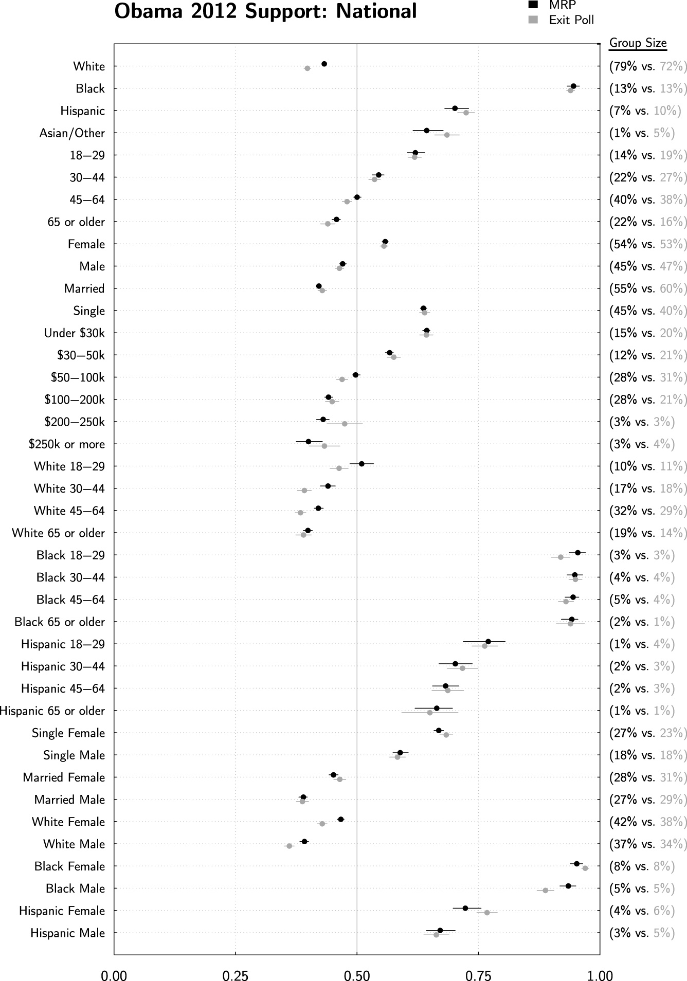
Figure 1 compares standard exit poll estimates (in gray) to our MRP estimates (in black) for various demographic subgroups on a national level. The exit poll estimates are the reported results provided to various news organizations on election night by Edison research.Footnote 10 We compute confidence intervals assuming simple random sampling, given the reported two-way vote share and sample size of the poll. In truth, these confidence intervals should be larger to account for the more complex sampling design, but data to compute these more complicated estimates are not publicly available.
The MRP estimates were constructed using the method described above. Because Catalist’s database indicates who voted in the 2012 election, it is trivial to produce poststratified Obama support estimates among 2012 voters, and it is equally trivial to create separate estimates for different subgroups—such as estimates for different geographies and subgroups within those geographies. In doing so, we compute estimates that are conceptually similar to the exit polls. We also draw 95% credible intervals for all of our estimates using the 100 sample draws from the model. As a result, we propagate sampling and modeling uncertainty through all of our estimates.Footnote 11
The dominant takeaway from Figure 1 is that the national MRP estimates are very close to the exit polls. There is a strong association between race and voting preferences—African Americans supported Obama at 94% according to both sources and Hispanics were at 70% and 72% for the exit polls and MRP, respectively, within the margin of error for each estimate.
MRP estimates (in black, with 95% credible intervals) are compared to standard exit poll estimates (in gray, with naively computed 95% confidence intervals). The vertical red line is provided as a reference, indicating overall Obama support. Estimates are quite similar at the national level, despite the fact that the exit polls were not used in any way to inform the MRP estimates. This provides face validation for the MRP method.
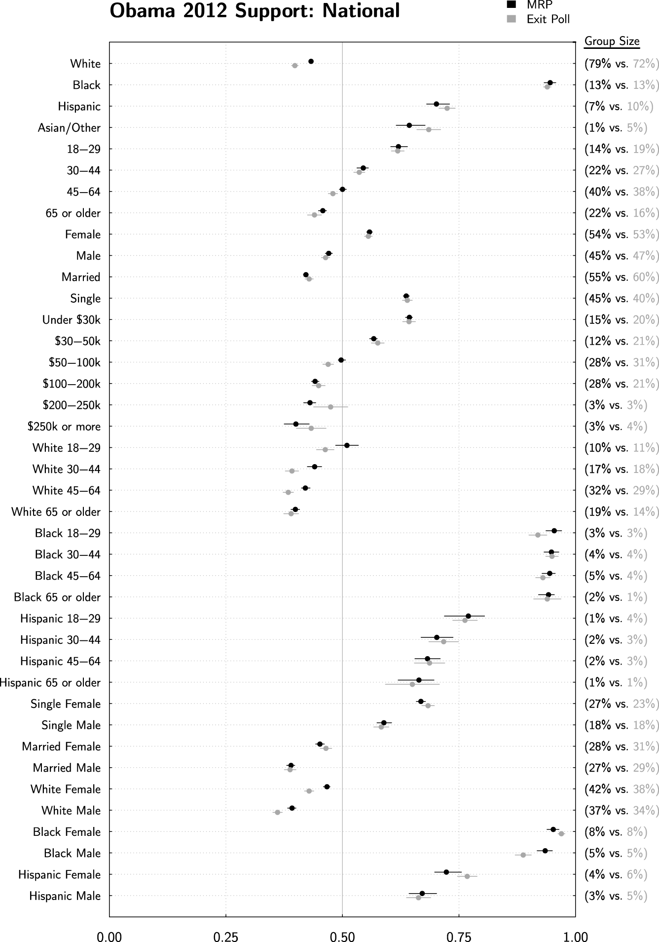
MRP has slightly higher Obama support levels among white voters—43% as compared to 40% in the exit polls. The MRP estimates are precise here, leading to an estimate that is statistically significantly different than the exit poll. But how could this be, given that both MRP and the exit polls add up to the final true vote total? The change is accounted for by different estimates of the white proportion of the voting electorate, as indicated on the right of the plot. According to Catalist’s data, 78% of the electorate was white, in comparison to 72% for the exit poll. When considering the group sizes and estimated support levels together in tandem, both the exit polls and MRP add up to the same final number.
It is worth stepping back and considering why these estimates might be different. Exit polls are surveys that rely on sampling and weighting strategies, both of which have experienced increased levels of scrutiny in recent years due to problems in their resulting estimates. Catalist collects data directly from each Secretary of State’s voter registration list. Although it is tempting to say, then, that the Catalist numbers are correct, we note that, in most states, Catalist’s race designation itself comes from a statistical model. Ansolabehere and Hersh (Reference Ansolabehere and Hersh2012) show that Catalist’s race model is quite accurate, but it is, of course, not perfect.Footnote 12 To extend the critique further, Catalist’s matching system, though again very accurate, does not capture everybody in the database with 100% accuracy. For this reason, we are agnostic as to which is the “better” estimate. Instead, we note that both estimates are indeed very close to one another, and we interpret the MRP estimate as a supplement to existing exit polls. This interpretation extends to the remainder of our results.
To continue along Figure 1, we see that most differences between MRP and the exit polls are statistically indistinguishable or very close to zero. Where they are different, it is only by a few percentage points, and the general characterization of all of the major trends are essentially exactly the same. Young voters were more likely to support Obama, as were women, single people, and lower income families. When we view the various two-way interactions that are available in the exit polls, we see that our MRP estimates are also essentially the same.Footnote 13
This provides a great deal of face validation to our MRP estimates. The exit poll data were not used in any way to inform our estimates, and still we ended up with almost exactly the same results at the national level.
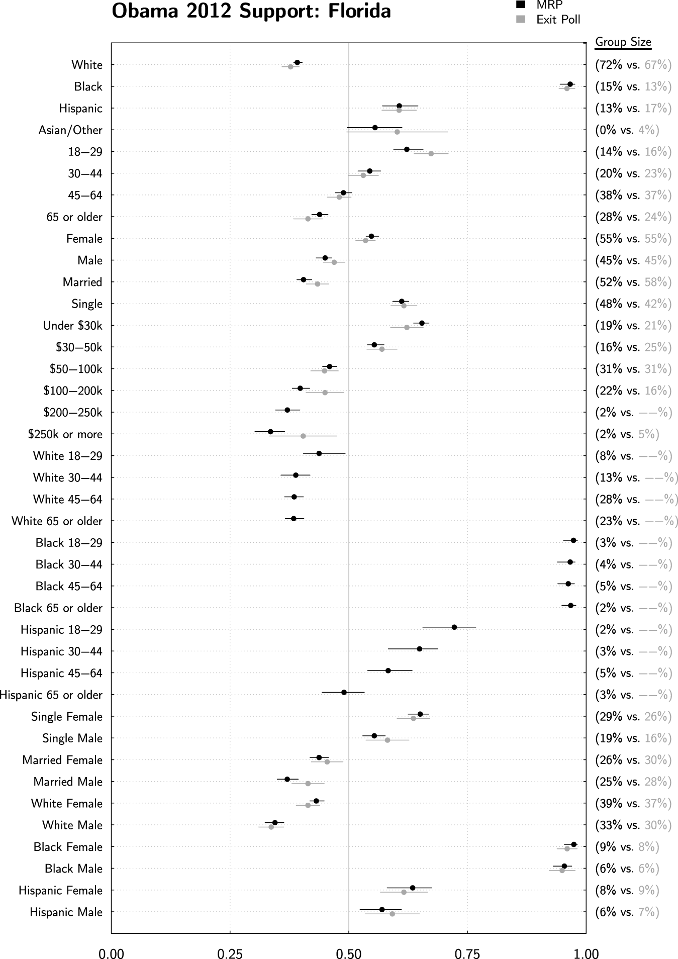
MRP estimates are trivially extended to the state level, here being compared to exit polls in Florida. Again the MRP and exit poll estimates are nearly identical, and at times, they are quite different than the national estimates, such as for Hispanics. Age/race interactions were not reported by the exit polls due to the small sample size, but they are easily estimated using MRP.

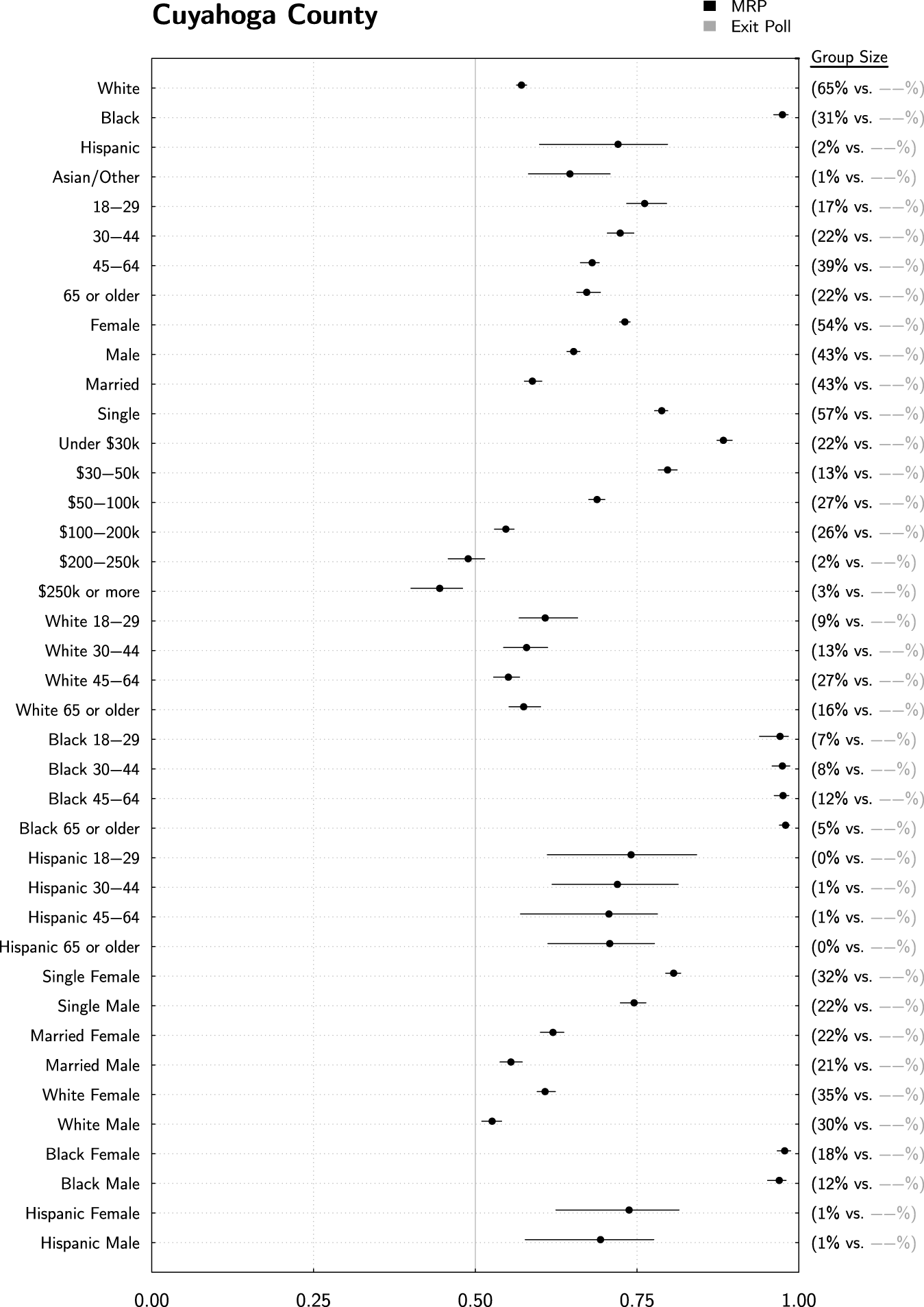
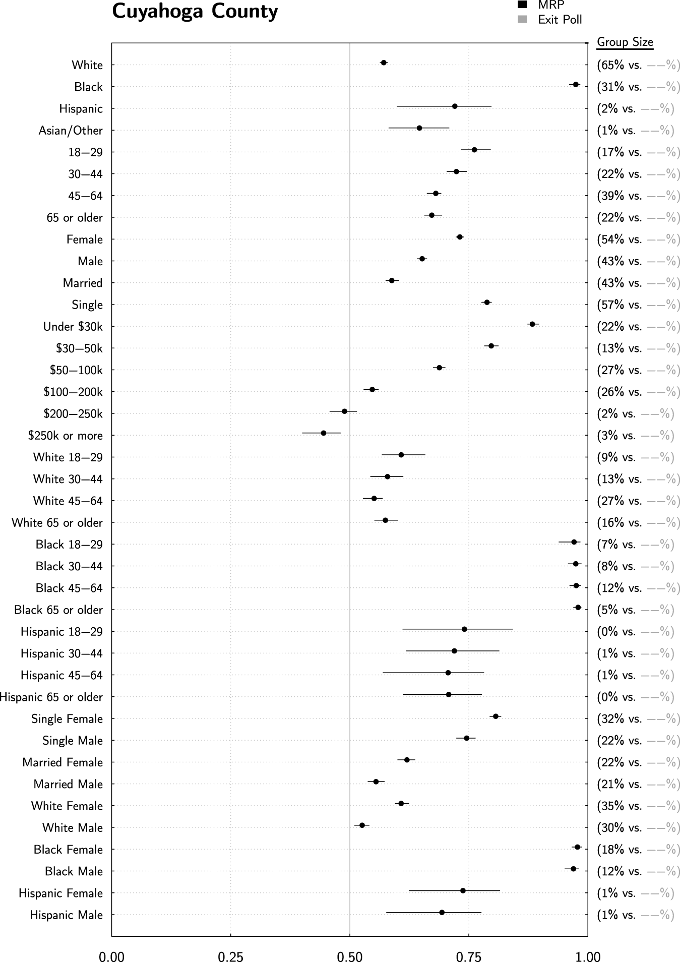
MRP estimates can be used to construct pseudoexit polls for geographies at the substate level. Here we show estimates for Cuyahoga County in Ohio, home of Cleveland and consistently an important indicator of Democratic support in this important battleground state. Caution should be used when projecting to substate geographies, however, because not all substate indicators are explicitly included in our statistical model. Still, our estimates appear reasonable.
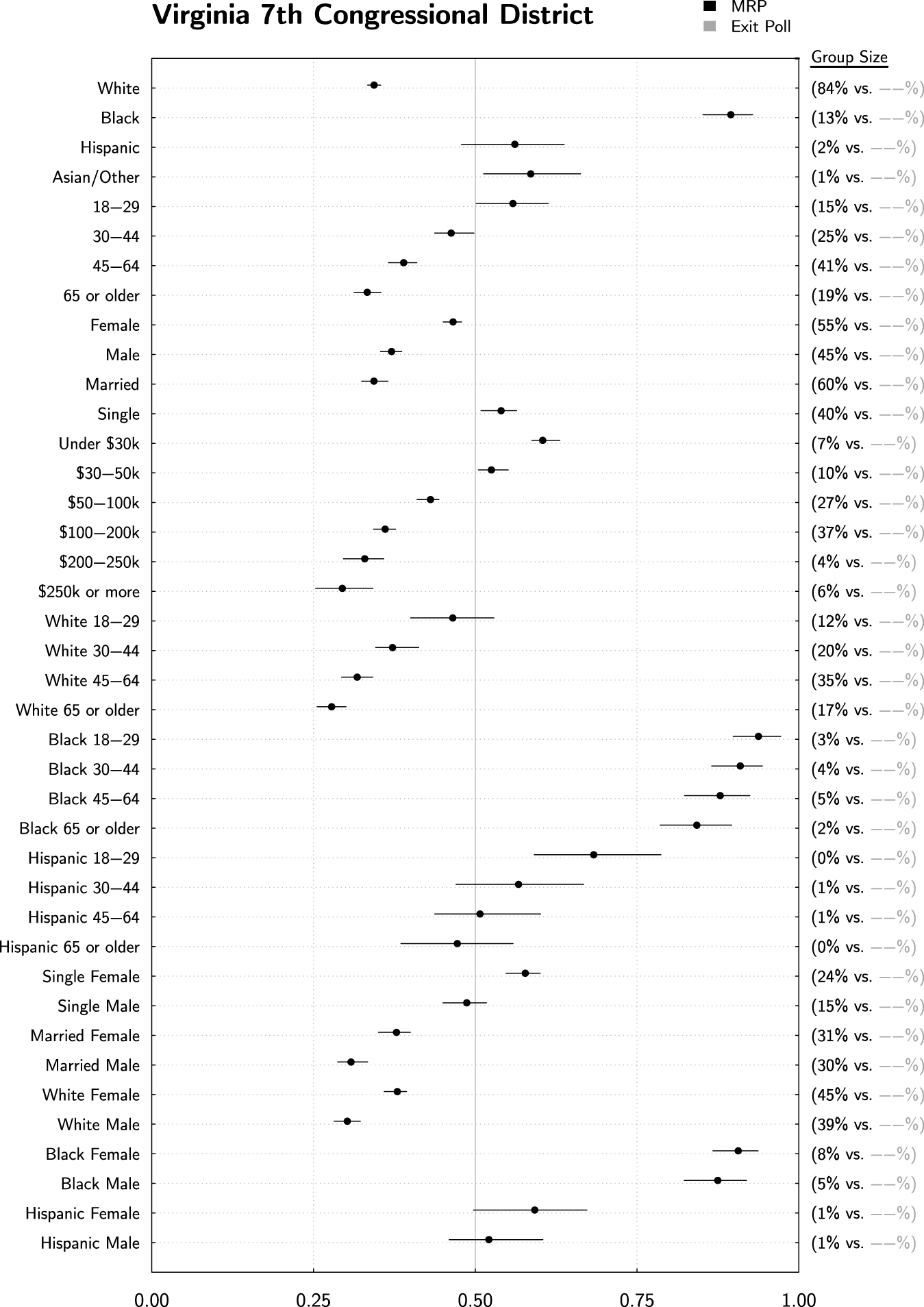
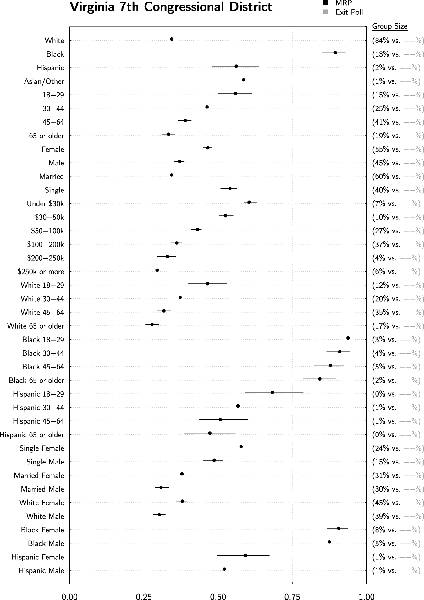
Catalist’s database keeps track of most relevant political geographies down to state legislative districts and precincts. Here, we show estimates for former US House Majority Leader Eric Cantor (R)’s district. These estimates may be helpful for scholars studying representation or any other area where these behavioral estimates might be useful and not otherwise available.
These similarities extend to state-level inferences, as shown, for example, for Florida in Figure 2. Again, almost all differences between MRP and the exit poll are essentially zero or very small. They are also at times quite different from the national estimates. Note that Obama support for Hispanics has now dropped to 61% for both the exit poll and MRP estimates, in part due to the larger Cuban population in Florida. For the MRP estimate, this change is reflective of four things: (1) a state intercept which shifted all estimates in the state by a similar amount (on the logistic scale); (2) county-level intercept shifts which accomplished the same thing on a county level; (3) state/race interactions in the model, which were included to allow just this type of variation; and (4) a different distribution of other covariates for the Florida Hispanic population as compared to the national Hispanic population. For example, the two-way registration rate among Hispanics is 75% Democratic nationally, compared to 58% among Hispanics in Florida alone. Because our model and poststratification account for all of these covariates simultaneously, our final estimates have the benefit of taking all of this additional information into account.
Also note the age/race estimates in Figure 2. The state-level exit polls did not report estimates for these groups within Florida, presumably due to lack of sufficient sample size. Our MRP estimates are easily computed and shown here. Comparing these estimates to others within Figure 2, as well as comparing to national estimates in Figure 1, builds confidence that these estimates are both reasonable and specific to Florida, for the same reasons as just stated.
This exemplifies one of the main contributions of our approach—namely, the ability to produce reasonable estimates for populations where exit polls either do not have sufficient sample size or where exit polls do not exist at all. Cost and complexity are leading fewer and fewer states to conduct exit polls. Our approach produces inferences for all states as well as substate geographies. Figure 3 displays our pseudoexit poll for Cuyahoga county in Ohio. Ohio is perennially an important battleground state, and Cuyahoga, which encompasses Cleveland, is always a stronghold of Democratic support and an important county in deciding who will win the state (and usually the country). Our approach easily leads to voting estimates for the county that are not calculable by any other means. We can easily see, for example, that 31% of the county is African American, supporting Obama at 97%. A majority (64%) is white, with an estimated 57% Obama support. Moving beyond race, we see that there is a substantial association between income and voting here, with a 43 percentage point gap between the richest and poorest group in Cuyahoga (45%–88%). Similarly, Figure 4 displays our estimates for Virginia’s 7th Congressional District, home to former Majority Leader Rep. Eric Cantor (R). For scholars interested in representation on the Congressional level, these types of estimates may prove valuable. Catalist keeps track of political geographies down to precincts and state legislative districts, and so these types of estimates can be drawn down to those levels as well.
With that said, a word of caution is in order regarding the use of our estimates within these small geographies. For national- or state-level estimates, our model explicitly incorporates parameters to account for differences reflected in the survey data—in other words, if there is a difference between Florida and the rest of the country, there is a varying intercept explicitly included in the model to capture that difference. When we go to the substate level, our estimates will avoid systematic error only to the extent that variation in voting patterns at that substate level is captured by the covariates that we have included in our model. If there is something special and different happening in VA-7 that is not reflective of the underlying distribution of the population as reflected in our model’s covariates, then that difference will be missed by our model and our final estimates. This word of caution indeed applies more generally—not just to geographies below the state level but to any subgroup that is defined by covariates not explicitly included in our model.
We should note that if we were particularly interested in Congressional Districts, we could in fact alter our statistical model to include terms to explicitly account for them. We refrain from doing so here because this would add a substantial number of additional parameters to the model.
Despite this limitation, we conjecture that these estimates can still be quite useful, even for small geographies and subgroups that are defined by characteristics not explicitly included in the model. Even in these cases, the estimates capture the impact of all the covariates that are included—all of the demographic, geographic, and political variables shown in Table 1—and they account for the underlying joint distribution of all of those covariates in simultaneity. Although those factors alone do not capture all variation for these small subgroups, they should still capture quite a bit. In cases where it is difficult or impossible to get any estimates at all, these imperfect estimates could be used as a reasonable approximation.
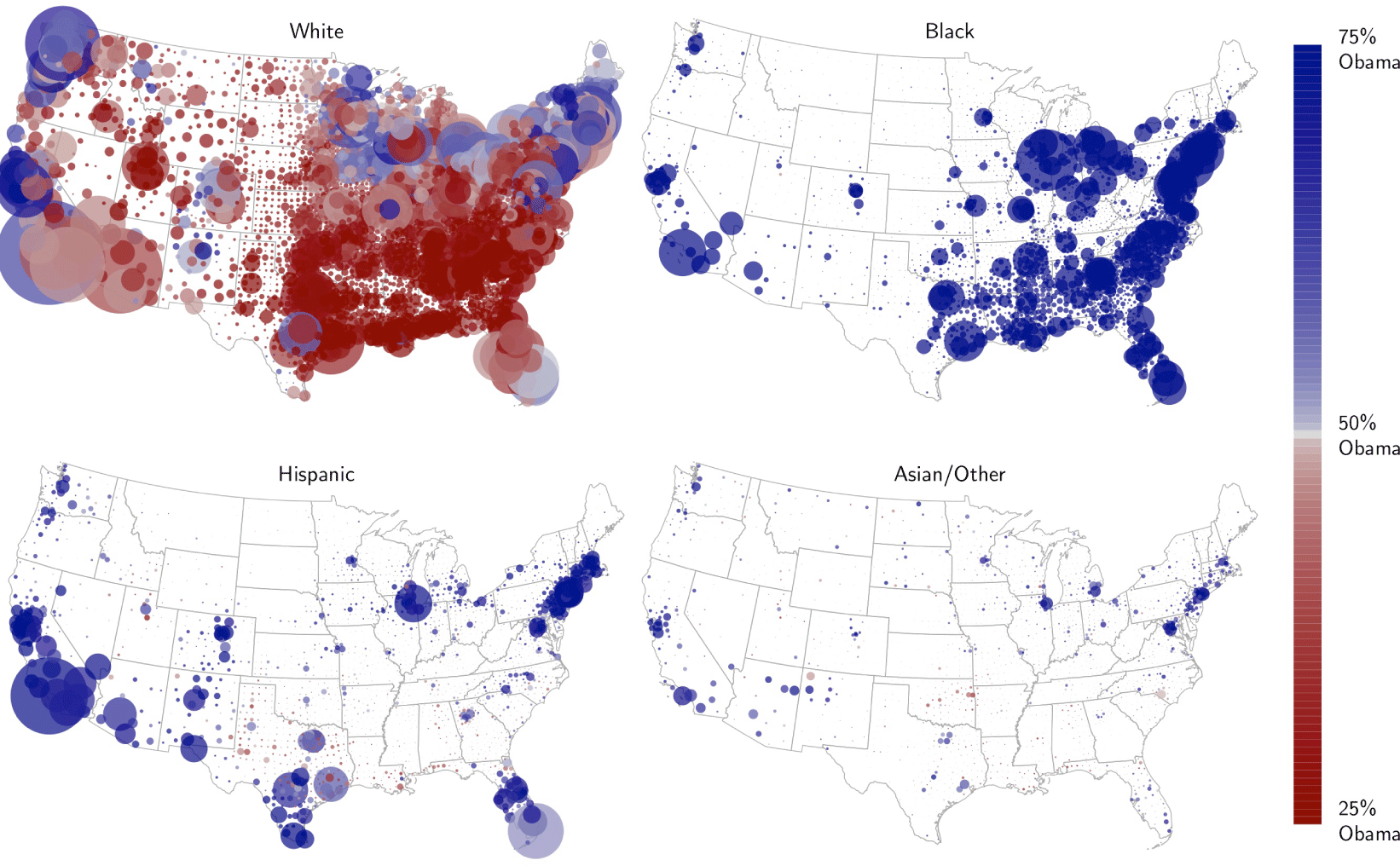
Small area estimates for racial voting trends, broken out by county. Each county is shown as a bubble, with size indicating number of 2012 voters in order to draw attention toward densely populated groups and color indicating Obama support. These maps confirm and clarify a number of widely discussed trends—Southern Whites voted overwhelmingly against Obama and African Americans supported him all over the map. High-population Hispanic areas had high levels of Obama support, but smaller Hispanic areas, particularly in the South, were more Republican. This was also true among Asians and other races. Interestingly, Hispanic support in Texas and Florida was lower than the national average, even in high-population areas.

3.2 Small Area Estimation
Small area estimation approaches refer to model-based methods used to derive inferences for small groups where “direct” design-based survey estimates are not appropriate. Direct estimates are usually design-based, in that they make use of survey weights, and the associated inferences (standard errors, confidence intervals, etc.) are based on the probability distribution induced by the sample design. In contrast, small-area methods use auxiliary data available at the small-area level to make predictions at that level (Rao Reference Rao2005). Rao defines a domain as “large if the domain sample size is large enough to yield direct estimates of adequate precision; otherwise, the domain is regarded as small …we generally use the term ‘small area’ to denote any subpopulation for which direct estimates of adequate precision cannot be produced” (Rao Reference Rao2005, p. xxi).
Our method clearly falls under this umbrella term. To the extent that small-area estimates are useful in political science research, methods such as the one discussed here are necessary, due to the lack of precise direct survey estimates for geographies even as high as the state level, and particularly for subgroups within states or smaller geographies. In the previous section, we gave a number of examples of small-area estimates. In this section, we provide a few additional illustrations.
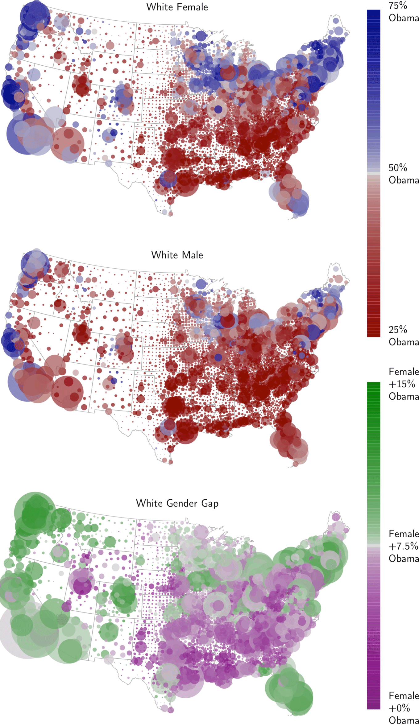
First, consider Figure 5. Here, we show Obama support estimates for every county in the lower forty-eight states, broken out by race. Each county is shown as a bubble, with size indicating number of voters in 2012 and color indicating Obama support, censored at 25% and 75%.Footnote 14 These maps confirm a number of known trends—Southern Whites voted overwhelmingly against President Obama, as seen in the sea of dark red all over the South. Indeed, the only counties that appear slightly blue in the top-left are near Miami and Austin. African Americans supported Obama overwhelmingly and in all geographies.
For Hispanics, we see high levels of Obama support in high-population Hispanic areas, especially California and New York. Note, however, that Hispanic support is lower than the national average in Texas and Florida, mirroring results from our earlier exit poll comparison plots. Interestingly, we also see that Hispanic support appears to be substantially lower in geographies with a small number of Hispanics, particularly in the South. This is also true for Asian/other races. We will revisit this data shortly.
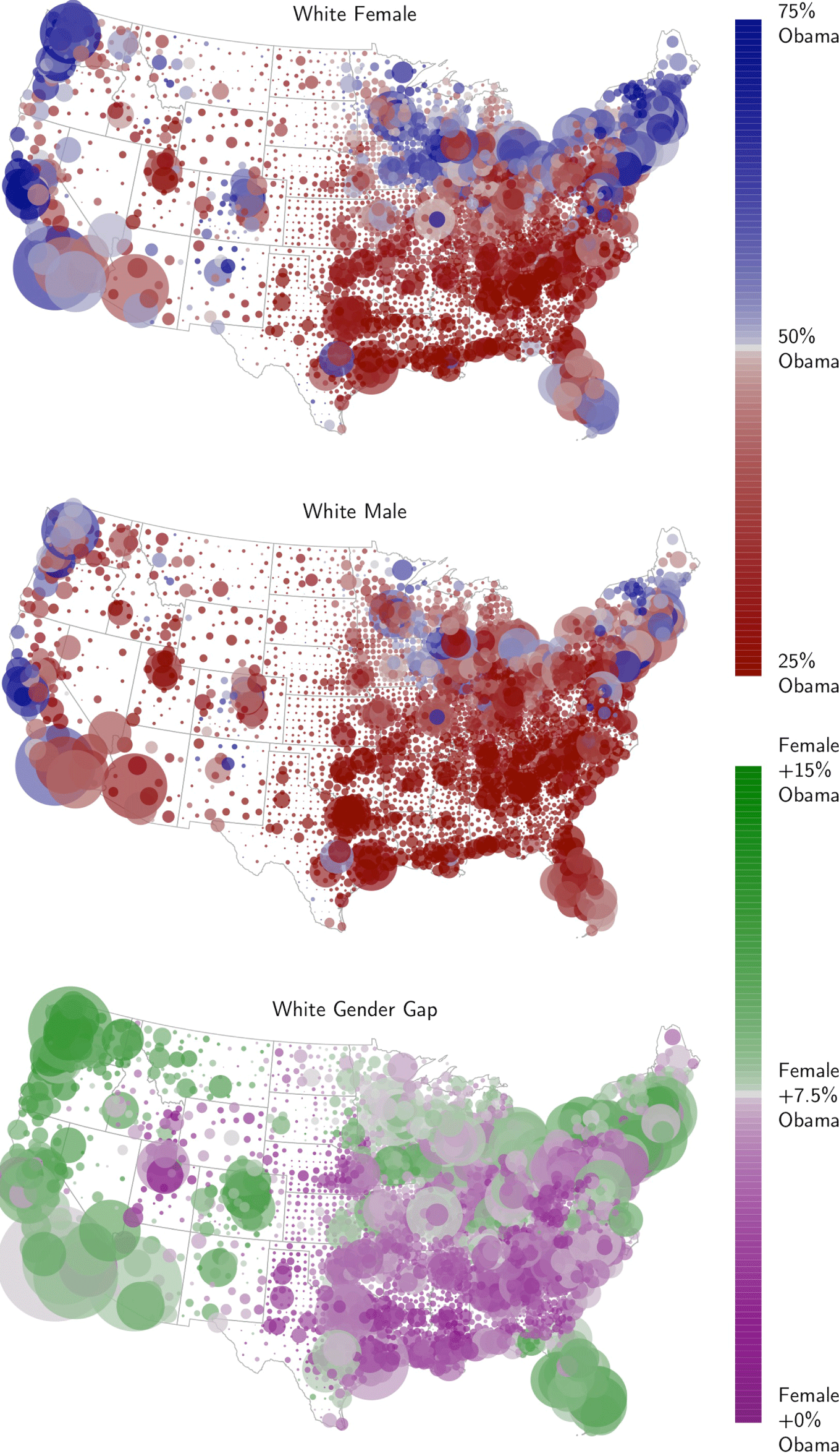
In our framework, we are not limited to looking at one covariate at a time. In Figure 6, we illustrate the preferences of white voters in slightly more detail, now conditioning on gender. Here we can see aspects of the much-discussed gender gap—namely, that it seems to exist in the North and West but not in the South. Another interpretation of this data is that voting among white males is relatively consistent across the country, while the familiar geographic voting trends among whites is primarily associated with different voting rates among women. In other words, white males as a whole generally voted against Obama, all over the country. The only notable exceptions are in a few places in the Northeast, the West coast, and around Chicago. Among white women, Obama enjoys considerable support in those places and in other areas as well. Indeed, among white voters, familiar geographic trends appear to be driven primarily by the voting preferences of women.
The gender gap among white voters. White males voted against Obama fairly consistently, with only a few exceptions. White females are more varied, following geographic trends that election analysts have grown accustomed to seeing—namely, more Democratic support in areas outside of the South. The difference between the two is plotted at the bottom.
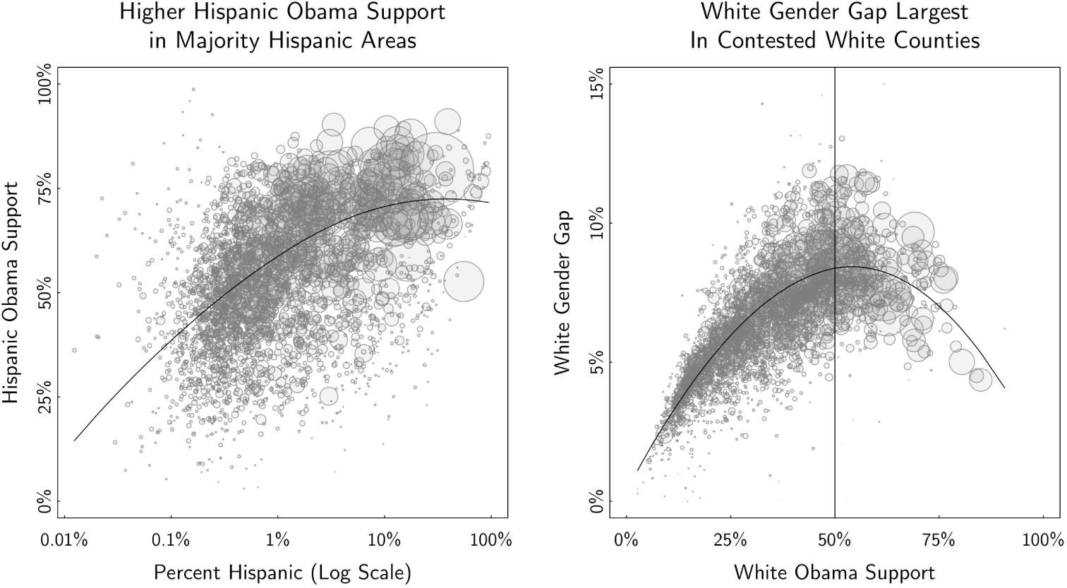
Trends from the last two maps are shown here as scatter plots. (L) We see an association between higher Hispanic density and higher Hispanic support for Obama. (R) Strongly Republican counties are homogeneous, as are the small number of white Democratic strongholds. The white gender gap is, somewhat tautologically, most pronounced in contested white counties.
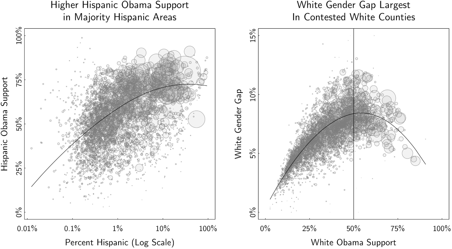
Figure 7 examines these two trends as scatter plots, with each bubble again representing a single county and size reflecting the voting population size. On the left, we see the earlier trend about Hispanics more clearly—majority Hispanic areas feature more Hispanic support for Obama, while it seems that areas with a small population of Hispanics tended to vote for Romney. On the right, the gender gap is plotted against overall support, among white voters only. Strongly Republican counties are quite homogeneous, in that there is essentially no gender gap whatsoever. This is also roughly true for strongly Democratic counties, although these do not really exist among white voters alone. The largest gender gap is seen in moderate or contested counties, here defined as places where the white vote is close to 50/50.
We see two possible interpretations to this data. On one hand, this can be seen as a function of modeling vote choice on the logistic scale—a single “gender effect” applied on the logistic scale will imply a larger effect at the midpoint of the logistic curve. On the other hand, nearly all binary models of vote choice are done on the logistic scale in part as an explicit attempt to see these sorts of differences. By looking at the results of our estimates in this way, as opposed to a single coefficient, we more clearly see the trends that our model imply, which are particularly salient when we consider all of the other covariates and interactions included in our model. Indeed, from a substantive perspective, this plot seems to make a great deal of sense. In Republican strongholds like the South, white voting preferences are homogeneous. This is similarly true in the few white Democratic strongholds (big cities like New York, San Francisco, Seattle, Chicago, and Washington DC, along with much of the Northeast). Everywhere else, where white voting is more moderate, there are much clearer differences between genders.
We make no claims about causal direction here—perhaps women in Republican strongholds (conversely, men in Democratic strongholds) are influenced by their neighbors to promote homogeneity of voting; conversely, perhaps higher Democratic support among women leads to more moderate areas in general. Unfortunately, our observational data are insufficient in answering these deeper causal questions.
Indeed, we do not attempt to parse either of these trends any further, except to point out that they seem relevant toward examining various open questions in American politics. There is an active literature on minority voting habits and the effects of majority minority districts (Barreto, Segura, and Woods Reference Barreto, Segura and Woods2004), for example, questions which could benefit from these types of small-area estimates. These observational data could be used to supplement regression discontinuity designs, natural experiments, and other formal methods of causal inference.
4 Discussion
We have laid out a new approach to deriving public opinion estimates using MRP and voter registration databases. At a conceptual level, our approach is, in some ways, simply a survey adjustment procedure. Normally, the goal of survey adjustment is to allow inferences from the survey sample, of size
 $n$
, to approximate the distribution of the full target population, of size
 $N$
. Standard adjustment procedures, such as survey weighting, attempt to correct for noncoverage in the sampling frame and differential nonresponse rates through a single model. The direction of the correction is, almost exclusively, to alter the sample to match the population.
We turn this on its head, by taking the survey sample as it is, and using our statistical model and poststratification to project inferences from the sample onto the full
 $N$
target population itself. We can do this because, through the voter registration database, we have access to data about the target population in much more detail than was previously possible. In other words, because we can observe the full
 $N$
of the target population directly, with many more important covariates available, we are less interested in altering the
 $n$
survey responses than in using them to properly project our inferences to the full
 $N$
database.
Both approaches require a model—in traditional procedures, the sample is collected and nonresponse is modeled conditional on covariates. Then the quantity of interest (QOI) is examined, assuming nonresponse was modeled properly. This is convenient because it only requires a single model (the nonresponse model), and once that is done, each QOI can be examined naively in a computationally inexpensive manner, i.e. through simple calculation of proportions. Assuming this is all done properly, results are unbiased, but the variance of these inferences can be high, sometimes prohibitively so, especially in small-area estimation problems. In contrast, our process models the QOI directly on all of our covariates and then poststratifies inferences onto the full
 $N$
individuals themselves. We automatically correct for noncoverage and nonresponse, conditional on our auxiliary covariates, at the same time that we are projecting our inferences. Once this is done, again naive techniques such as proportions can be used. Resulting estimates have lower variance than design-based methods, especially in small-area estimation problems, appearing stable and plausible to a high degree of geographic and subgroup specificity. Auxiliary data available in the voter databases can also facilitate powerful and informative secondary analyses.
Our method is particularly attractive when used in conjunction with voter registration databases. Instead of weighting surveys to the census or to exit polls, these databases provide (1) a more accurate picture of the registered voting population; (2) the ability to construct a verified voter population through the use of past voting records; and (3) the ability to use powerful and stable political covariates such as party registration in the survey correction procedure.
We have argued that the resulting estimates provide a good supplement to existing exit polls. It is instructive to compare our process to the type of informal analyses that are typically done after an election. Postelection analyses often proceed by examining exit polls, geographic election returns, or both. Demographic and partisan trends are parsed out from the exit polls, and geographic trends are loosely related to demographic criteria through census data. With these data points in hand, pundits, election analysts, and scholars form a story about how different groups voted in the election and how those voting choices relate to the messaging and preferred policy choices of the candidates. In our view, analyses of this kind, while informal and of varied quality, are generally a reasonable approach. Our approach is fairly similar—we are interested in understanding who voted for which candidate. The benefit of our method, though, is that we take all of these disparate data sources—polling, geographic election returns, and population data—and put them together under a single well defined framework in order to achieve the best possible estimates.
There are many benefits to this approach, but we also caution the reader as to some of the difficulties and open research challenges. First, using voter registration databases as done here necessitates a substantial investment in statistical and “big data” expertise. These databases do not fit on a laptop, and moving into the realm of computations involving hundreds of millions of records is quite a different skill set than the one required for thousands of respondents in a survey.
Second, despite the improved data quality that is provided by vendors like Catalist, data coverage remains variable in different geographies. This could potentially bias results if not treated properly. For most of the data presented in this paper, our statistical model explicitly accounted for the covariates of interest—when that is the case, the statistical model should adjust for any such differences to the extent that those changes are apparent in the survey data and ignorability assumptions are not violated. But when we step outside of that framework, our results are more highly dependent on data quality and coverage. This is a generally important point that should be considered whenever conducting analyses using voter registration databases.
Third, inferential uncertainty is an area that requires a great deal of additional research. We successfully propagated sampling and modeling uncertainty in our modeling parameters through our entire process. But this is certainly not the only source of uncertainty in the process. Additional considerations include uncertainty introduced through (a) measurement error from Secretary of State data; (b) Catalist’s matching system, which does not guarantee that matches are 100% accurate; (c) statistical covariates, such as income or education—we have treated them as fixed in this paper, but they themselves are at times built from statistical models and thus have uncertainty in and of themselves; and (d) modeling choices—here we used a single model, namely a flexible multilevel model defined very specifically as described earlier; it is important to understand whether and under what conditions our estimates could change dependent on model specification.
Fourth, the observant reader may have noticed that the survey we used in this paper covered a long stretch of the campaign, from March through November. This was done out of necessity because we needed sufficient sample size to fit our complicated statistical model. However, one of the main goals of political polling is to look at changes over time; and, indeed, the question of how these estimates might change over time within a single campaign is still open and quite important.
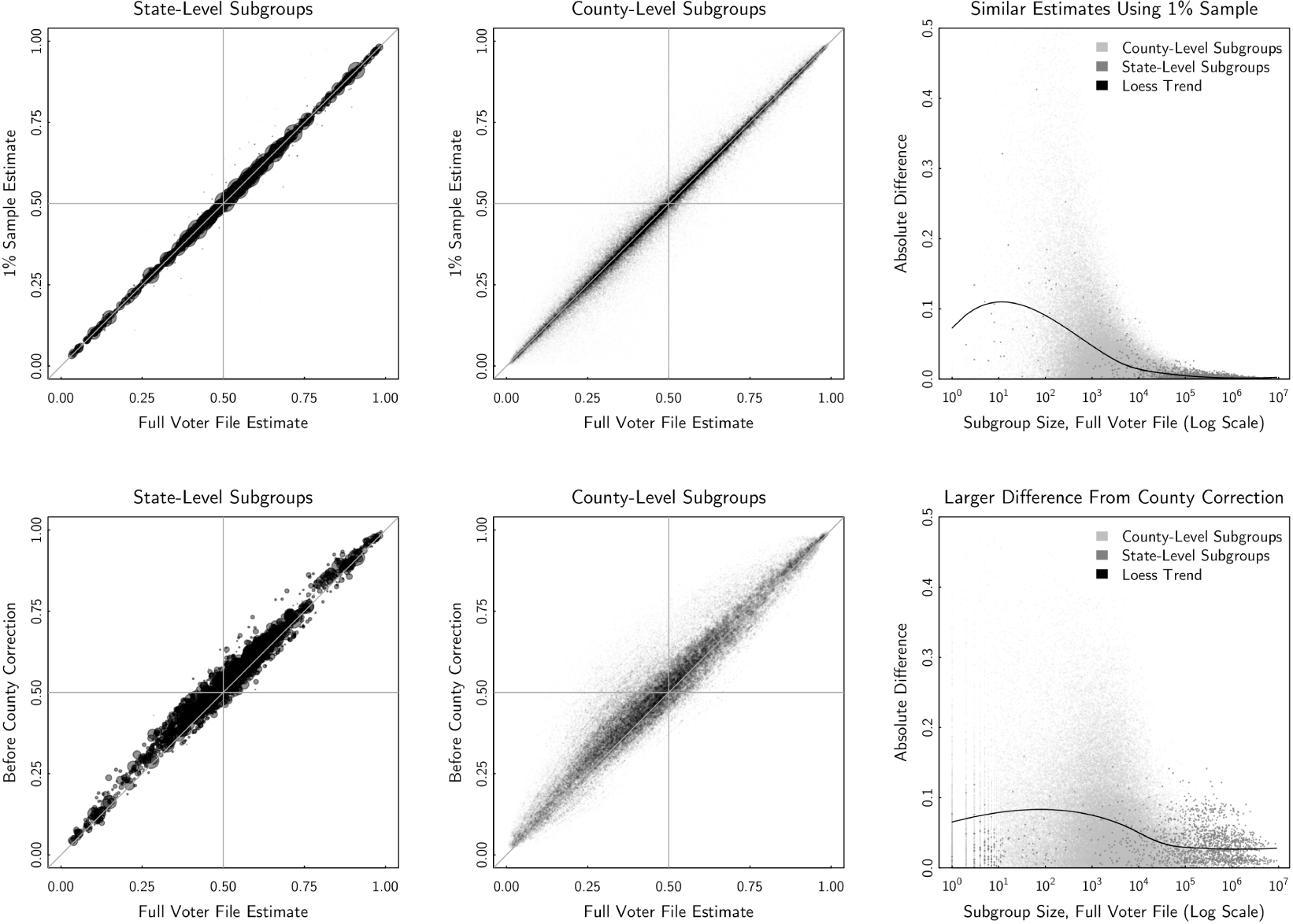
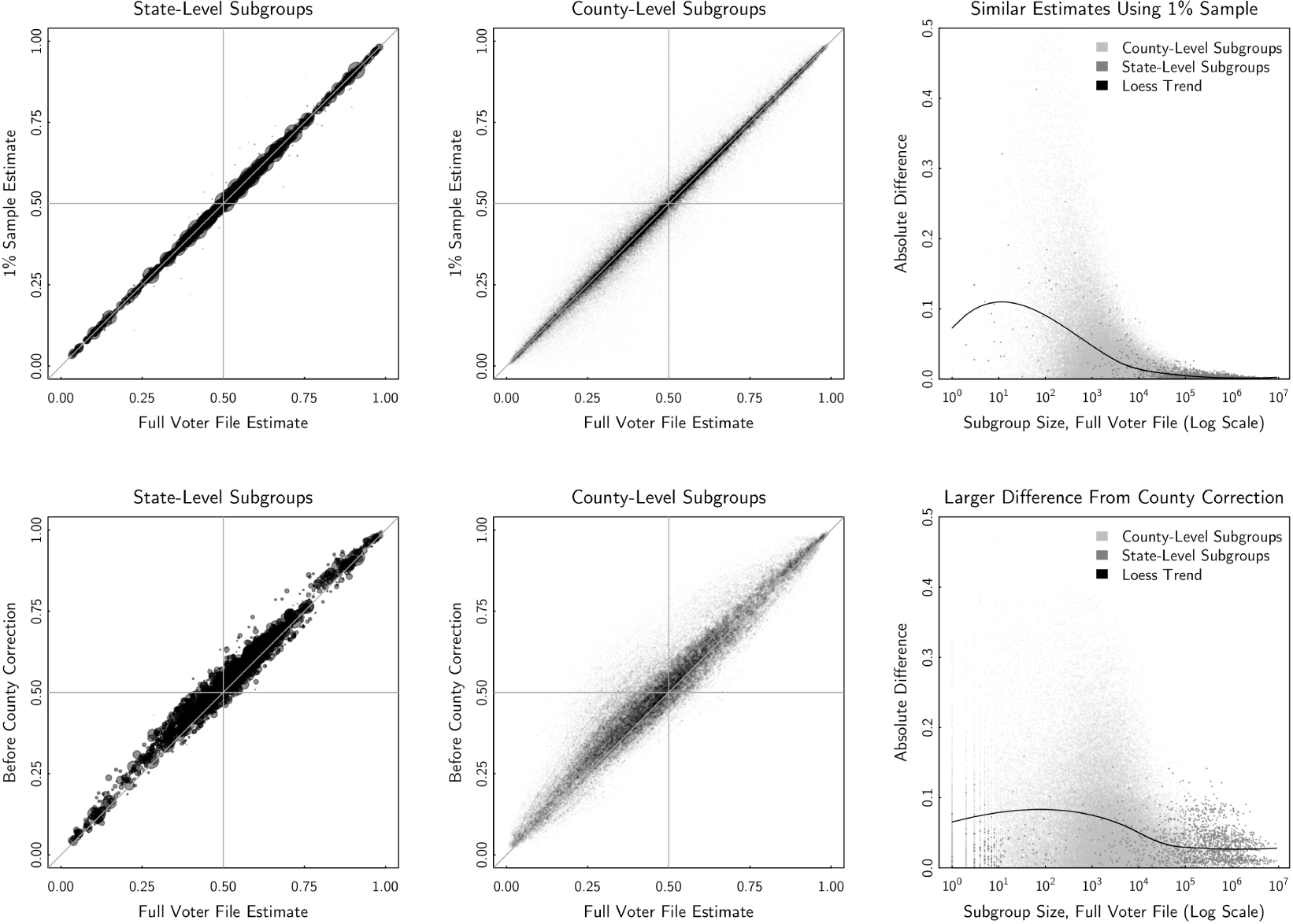
Fifth, a related question involves the importance of the intercept correction step. Our estimates in this paper had the benefit of knowing the “right answer” through county-level election returns, for the population as a whole. This is fine in a postelection context, but it is a somewhat ad-hoc correction that is not generally available for most estimates of public opinion. What about the preelection context? The bottom panel of Figure 8 in the Appendix compares precorrection estimates to our final corrected estimates and shows that the precorrection estimates were biased slightly upwards. Our sense is that has to do with different data quirks across states in the voter registration file. For example, in West Virginia, despite the state voting strongly Republican in recent years, especially at the federal level, Democrats have a 19 percentage point advantage in registration.Footnote 15 Party registration is strongly associated with vote choice nationally, and there are only 134 survey responses from West Virginia, so the interaction term that might correct for this in the multilevel model does not have enough data to make this correction in the model alone. Given more survey responses, the multilevel model might be sufficient in making this correction; more likely, some custom solution that accounts for these known data discrepancies may also solve these problems.Footnote 16 This is an important area of future research.
Sixth, we have not addressed how to look at multiple survey measures at the same time. A common use of survey data is to produce cross-tabs, i.e. joint distributions involving multiple questions from the same survey—Obama support separated by self-reported ideology, as an example. Although our method can create estimated inferences for survey measures one at a time, it is unclear how to combine those estimates due to the probabilistic nature of our resulting inferences. In the notation of our statistical model,
 $y$
is a discrete 0/1, but
 $\unicode[STIX]{x1D703}$
is a probability. There are various possible solutions—such as binning the continuous
 $\unicode[STIX]{x1D703}$
s into discrete groups, integrating over all possible values, or modeling the joint density across multiple dimensions—but the properties of these estimators still need to be worked out. A related problem involves modeling nondichotomous outcomes, such as third party candidates. Here, again, a possible solution is modeling the joint probability of the three outcomes.
With these caveats in mind, we emphasize that this is an area of exciting opportunity for public opinion as a whole. MRP is an improvement over standard weighting methods in extrapolating from small survey datasets to larger population datasets, and we show that MRP estimates are reasonable even for very small groups, given the appropriate population-level dataset as a poststratification target. This facilitates detailed analyses that were very difficult, if not impossible, to perform otherwise, such as producing exit polls for electorally important counties. This general approach can be extended to other areas where estimates from a small and nonrepresentative dataset are to be projected onto a larger population database and where both have a rich and overlapping set of modeling covariates to produce a reasonable model. Voter registration databases include particularly powerful covariates, such as registration and vote history, to supplement survey data and allow for interesting supplemental analyses. Although it is technically challenging to produce these types of estimates at the moment, the continued advancement of computational and data storage resources ensure that it will become easier to do this type of work in the future. It is incumbent upon survey methodologists to keep up with these new opportunities and develop the newest and best methods to take advantage of them.
Data Availability Statement
The replication materials for this paper can be found in Ghitza and Gelman (Reference Ghitza and Gelman2019).
Appendix
Comparison of estimates. The top panel compares poststratified using the full Catalist voter file vs. a 1% sample. Estimates from the 1% sample are noisy for small groups but are around or below 1 percentage point, on average, for groups with greater than 10,000 registered voters. The bottom panel compares final estimates to precounty-correction estimates. Here the differences are larger, as described in the Section 4.
Catalist’s full dataset is not generally available to scholars, but they do offer a 1% sample via an academic subscription. Scholars who want to apply our method may be interested in how it performs when poststratifying against the 1% sample.Footnote 17
The top panel of Figure 8 compares estimates poststratified using the full voter file (as shown in the bulk of the paper) to those poststratified using the same method on the 1% sample alone. The top-left and top-middle panels show state- and county-level subgroups, with the size of each bubble indicating the size of the group. In both cases, the two estimates are shown to be highly correlated. The third panel shows the root mean squared difference between the estimates (full vs. 1%) as a function of subgroup size. For small groups, the differences can be large, but for groups sized greater than roughly 10,000 registered voters, the difference is around or below 1 percentage point, on average. One advantage of using the 1% sample is that it reduces the computational and storage necessities described in the Section 2.3 of the paper. Because the M database is 100 times smaller, operations should be much faster and easier to manage using this approach, at the cost of added variance to smaller subgroup estimates.
The bottom panel compares final estimates to precounty-correction estimates. Here the differences are larger, as the final estimates are lower, on average.