

1. Introduction
Anthony Hallam is well known for his pioneering work on the end-Triassic extinction. His work was the first to highlight the association of the biotic crisis with ocean anoxia and sea-level changes (Hallam, Reference Hallam1981; Hallam & Wignall, Reference Hallam and Wignall1999). Perhaps less appreciated, he was also the first to collect high-resolution carbon isotopic data spanning the extinction horizon (Hallam & Goodfellow, Reference Hallam and Goodfellow1990; Hallam, Reference Hallam1994; Morante & Hallam, Reference Morante and Hallam1996) and was therefore the first to identify what we now recognize as one of the hallmarks of the end-Triassic extinction: the negative δ13C excursion associated with the disappearance of the Triassic biota.
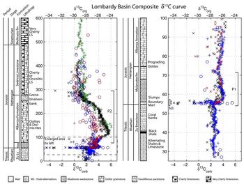
The stratigraphically abrupt drop in δ13C of carbonate and organic carbon coincident with the last occurrence of Triassic biota has now been identified in numerous, globally distributed Triassic–Jurassic boundary (T–J) sections (Hallam, Reference Hallam1994; Ward et al. Reference Ward, Haggart, Carter, Wilbur, Tipper and Evans2001; Hesselbo et al. Reference Hesselbo, Robinson, Surlyk and Piasecki2002; Galli et al. Reference Galli, Jadoul, Bernasconi and Weissert2005; Ruhl, Kürschner & Krystyn, Reference Ruhl, Kürschner and Krystyn2009; Ruhl et al. Reference Ruhl, Bonis, Reichart, Damsté and Kürschner2011; Greene et al. Reference Greene, Martindale, Ritterbush, Bottjer, Corsetti and Berelson2012). It has also been the focus of several modelling studies aimed at constraining the mass of Central Atlantic Magmatic Province (CAMP) -derived volatiles and/or volume of methane released (Beerling & Berner, Reference Beerling and Berner2002) as well as the associated impacts on ocean chemistry such as acidification (Berner & Beerling, Reference Berner and Beerling2007; Paris et al. Reference Paris, Donnadieu, Beaumont, Fluteau and Goddéris2012) and warming (Huynh & Poulsen, Reference Huynh and Poulsen2005). These models, which focused on the boundary interval, assumed a complete return to steady state and full recovery after the initial negative δ13C excursion. However, recently developed carbon isotope records extending through Hettangian succession have shown that the negative δ13C excursion is followed by a protracted interval of 13C enrichment (Fig. 1). This portion of the T–J carbon cycle perturbation has yet to be explored by modelling, leaving incomplete our understanding of the events associated with the end-Triassic mass extinction and ensuing recovery. Moreover, the recently developed high-resolution chronologies for CAMP activity (Schoene et al. Reference Schoene, Guex, Bartolini, Schaltegger and Blackburn2010; Blackburn et al. Reference Blackburn, Olsen, Bowring, McLean, Kent, Puffer, McHone, Rasbury and Et-Touhami2013), coupled to pCO2 estimates from proxy measurements on palaeosols interbedded with the basalts (Schaller, Wright & Kent, Reference Schaller, Wright and Kent2011; Schaller et al. Reference Schaller, Wright, Kent and Olsen2012), allow the investigation of the relationship between volcanic activity and 13C enrichment (and by inference, ocean chemistry) in unprecedented detail.
Carbon isotope record of the uppermost Triassic and lowermost Jurassic from the Lombardy Basin, Italy. This is one of the geochemically best-characterized sections presently available with both organic and carbonate carbon showing co-enrichments, an indication that the δ13C signal is primary in origin and representative of the original ocean water chemistry. The large negative excursion at the extinction (N1) is followed by a small positive excursion (P1) and a large protracted excursion (P2). Data from Bachan et al. (Reference Bachan, de Schootbrugge, Fiebig, McRoberts, Ciarapica and Payne2012). δ13Corg hollow circles, δ13Ccarb all other symbols.

Here we use a global biogeochemical box model to explore the carbon cycle consequences of CAMP-associated perturbations and to constrain the conditions under which the recovery from the end-Triassic mass extinction may have taken place. In particular, we attempt to answer the question of how pCO2 and ocean carbonate chemistry may have changed during the recovery and what bounds can be placed on their values in light of the δ13C records.
2. Model description
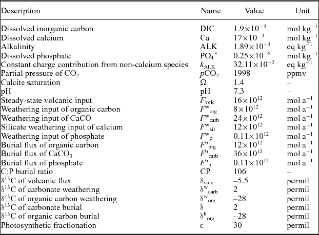
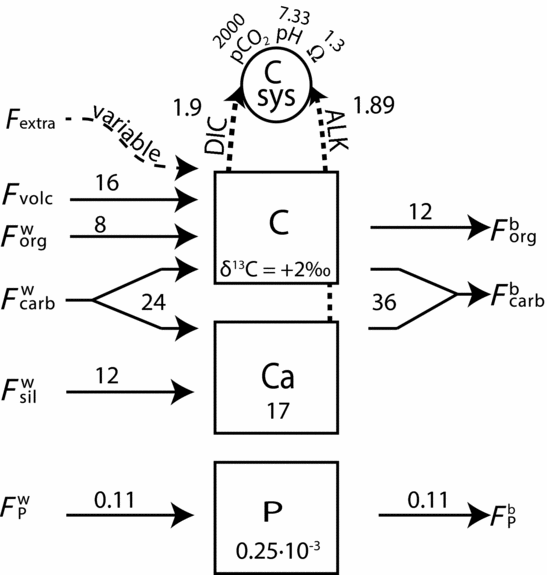
Our model comprises a mass box representing the total carbon in the ocean–atmosphere system, an isotopic-mass box representing the overall isotopic composition of that carbon, as well as boxes representing the total calcium and phosphorus in a well-mixed ocean (Fig. 2, Tables 1–3). Inputs to the boxes correspond to delivery of carbon and alkalinity from volcanism and weathering to the ocean. Outputs from the boxes correspond to the burial of calcium carbonate and organic matter from the ocean in marine sediments (Fig. 2, Table 3). In addition, the carbon box includes a variable F extra input by which we perturb the model.
Steady-state values for model fluxes and reservoirs. Flux values after DePaolo (Reference DePaolo2004) and Kump & Arthur (Reference Kump and Arthur1999). Dissolved calcium based on Horita, Zimmeerman & Holland (Reference Horita, Zimmermann and Holland2002) and pCO2 after Berner (Reference Berner2006). Magnitude of photosynthetic fractionation from Hayes, Strauss & Kaufman (Reference Hayes, Strauss and Kaufman1999). Concentrations of carbon, calcium and phosphate converted to masses using an ocean volume of 1.32×10²¹ L and salinity of 1.035 kg L−1. k ALK is the sum of charges from all cations excluding Ca2+.

Governing equations

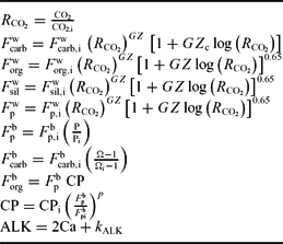
Weathering and burial feedbacks. Fluxes with w superscript represent weathering and b burial. Fluxes with i subscript are initial steady-state values. All others are time-varying values. Weathering feedback parameterization after Berner (Reference Berner2004): G = 3.3, Z = 0.09, Z c = 0.07.

Sketch of model. Ca and P boxes represent the oceanic reservoirs of calcium and phosphate, and the C box represents the ocean–atmosphere pool of carbon. Inputs and outputs correspond to weathering and burial fluxes of carbon, alkalinity and phosphate into and from the ocean. Csys denotes the carbonate system solver. Numbers in boxes and adjacent to DIC and ALK are concentrations in mmol kg−1; pCO2 is in units of ppm; and numbers on fluxes are rates in Tmol (1012 moles) per year. Flux names, descriptions and steady-state values given in Tables 1–3.

We set initial model attributes to match a postulated latest Triassic steady state (Table 1). The initial value of dissolved calcium (17 mM) was taken from Horita, Zimmermann & Holland (Reference Horita, Zimmermann and Holland2002) and the initial value for pCO2 (2000 ppm) from Berner (Reference Berner2006). Initial values for alkalinity (ALK, 1.8 mEq kg−1) and dissolved inorganic carbon (DIC, 1.9 mM) were chosen to yield the appropriate pCO2, together with the ocean calcite supersaturation commensurate with the modern whole-ocean average of 1.3 (Berner & Beerling, Reference Berner and Beerling2007). We used modern ocean volume (1.32×10²¹ L) and salinity (35 ppt) to convert concentrations to masses. The values for inputs and outputs from the boxes were taken from DePaolo (Reference DePaolo2004) and Kump & Arthur (Reference Kump and Arthur1999) and modified to yield a steady-state δ13C value of +2‰. The baseline magnitude of photosynthetic fractionation was taken from Hayes, Strauss & Kaufman (Reference Hayes, Strauss and Kaufman1999). A full list of the model steady-state attributes is given in Table 1.
In the model we calculate ocean chemistry parameters (pH, pCO2 and Ω) from ALK and DIC at every time-step using a carbonate system solver based on Zeebe & Wolf-Gladrow (Reference Zeebe and Wolf-Gladrow2001) and the code in Emerson & Hedges (Reference Emerson and Hedges2008). The values for ALK and DIC are determined from the calcium and carbon boxes, respectively. For simplicity, the contribution of all other conservative ions to ocean alkalinity is assumed constant.
Feedbacks in the model (Table 3) include a dependence of all weathering fluxes on pCO2 using the parameterization of Berner (Reference Berner2004), which includes a different weathering coefficient for carbonate rocks reflecting their increased susceptibility to dissolution compared to crystalline silicate rocks. Carbonate burial is set to be first-order dependent on the carbonate saturation state Ω, such that Ω > 1 results in carbonate burial and Ω < 1 results in carbonate dissolution (a negative flux). Phosphate burial is set to be first-order dependent on phosphate concentration. Organic carbon burial is set by the product of phosphate burial and the C:P burial ratio. The C:P burial ratio itself is set to be proportional to phosphate burial, resulting in a strong sensitivity of organic carbon burial to increased phosphate input.
The model is designed to address a medium range of deep-time perturbations: those that are longer than the rate of cycling of carbon between surface reservoirs, which is smaller than a few thousand years (ka), but shorter than the hundred million year (Ma) timescale of fluxes in and out of sedimentary reservoirs (e.g. Garrels & Perry, Reference Garrels, Perry and Goldberg1974). Consequently, we assume that the flow of carbon between surface reservoirs such as soils, land biota, atmosphere and shallow and deep oceans are in steady state and can be treated as one homogenous reservoir. Because of this assumption of steady state, the model is not suitable for simulating perturbations occurring on timescales shorter than the longest internal process, which is the mixing time of the oceans (on the order of a few thousand years; Broecker & Peng, Reference Broecker and Peng1982). We further leave the treatment of isotopic gradients between the shallow and deep ocean (Kump, Reference Kump1991) as well as spatial heterogeneities (Panchuk, Holmden & Kump, Reference Panchuk, Holmden and Kump2005) for future work. We also assume that the imbalance between organic and carbonate carbon weathering and burial is compensated by volcanic input, which is itself sourced by metamorphic degassing and reverse weathering of the excess burial. We therefore assume that the inputs and outputs are closed outside the model by cycling of carbon between sedimentary reservoirs. For readers interested in additional details or running the model on their own, the Matlab code is provided in the online Supplementary Material (available at http://journals.cambridge.org/geo).
3. Results
Below we present the model response to CO2 injections of three different durations: 20, 100 and 500 ka. We explore the effects of differing δ13C values of the injected carbon for the 20 ka perturbation, and discuss the impacts of changing the model parameters that control the sensitivity of organic carbon burial and attendant 13C enrichment for the other scenarios. We then assemble the model runs into a multi-perturbation scenario in an effort to fit the CAMP degassing chronology and δ13C record.
3.a. Single perturbation scenario
The magnitude, duration and isotopic composition of the volatile releases from CAMP activity are key variables in modelling the associated carbon cycle perturbation. Estimates for the magnitude of volatile release vary: Schaller et al. (Reference Schaller, Wright, Kent and Olsen2012) use a value of 3.5×10¹⁷ mol (moles) of CO2 to represent a single volatile release pulse and assume four of them for a total of 1.4×10¹⁸ mol; Berner & Beerling (Reference Berner and Beerling2007) use a value of 1.76×10¹⁸ mol carbon for the total integrated release; and Paris et al. (Reference Paris, Donnadieu, Beaumont, Fluteau and Goddéris2012) use, in addition to the value of Berner & Beerling (Reference Berner and Beerling2007), a low value of 1.2×10¹⁷ and a high value of 2.9×10¹⁸ mol for the total volatile release. These estimates are generally obtained by multiplying the average volatile load of basalt (0.6%) by the reconstructed volume of the province (<4×10 km3; McHone, Reference McHone2003) times the assumed degassing fraction (100%).
These estimates are likely conservative however, as they assume no interaction of the igneous province with the abundant rift and passive margin sediments through which the CAMP intruded. Geochemical evidence from distinctive, fine-grained domains within CAMP volcanic rocks in the southern Iberian peninsula yield elevated CaO and 87Sr/86Sr (Martins et al. Reference Martins, Madeira, Youbi, Munhá, Mata and Kerrich2008), suggesting a 2–10% assimilation of a pure CaCO3 end-member which would imply an order of magnitude increase in degassed CO2 over unadulterated basalt. Sills in the Amazonian basin intruding into carbonate and evaporite sediments have an average thickness of 500 m and cover an area of 1×10⁶ km2 (Marzoli et al. Reference Marzoli, Renne, Piccirillo, Ernesto, Bellieni and Min1999). Moreover, CAMP basalts abut coal bodies in the eastern USA (Robbins, Wilkes & Textoris, Reference Robbins, Wilkes, Textoris and Manspeizer1988), suggesting possible degassing of CO2 and thermogenic methane from coal (Ogden & Sleep, Reference Ogden and Sleep2012). The total magnitude of interaction between CAMP basalts and sediments is difficult to quantify, but if even a fraction of CAMP basalts had a similar magnitude of sediment interaction, the amount of carbon released by CAMP may have been substantially underestimated. Similarly, interactions with sediments could lead to an either more 13C-enriched or more 13C-depleted carbon isotopic signature of the evolved volatiles, depending upon the isotope composition of the sediments. Volatiles released from the interaction between basalts and coals (Retallack & Jahren, Reference Retallack and Jahren2008; Ogden & Sleep, Reference Ogden and Sleep2012) would have a δ13C value closer to −20‰ whereas interaction with carbonates would lead to a δ13C more positive than −5.5‰, possibly close to 0‰. A pulse of methane triggered by CAMP volcanism (Beerling & Berner, Reference Beerling and Berner2002) would have a value of −50‰ to −100‰ depending on whether the gas was thermogenic or biogenic in origin. Additionally, it is possible (though highly uncertain) that the emitted magmatic carbon itself may have been 13C-depleted through interactions with pools of isotopically light carbon in the mantle (Deines, Reference Deines2002; Cartigny, Reference Cartigny2010; Paris et al. Reference Paris, Donnadieu, Beaumont, Fluteau and Goddéris2012).
3.a.1. 20 ka release
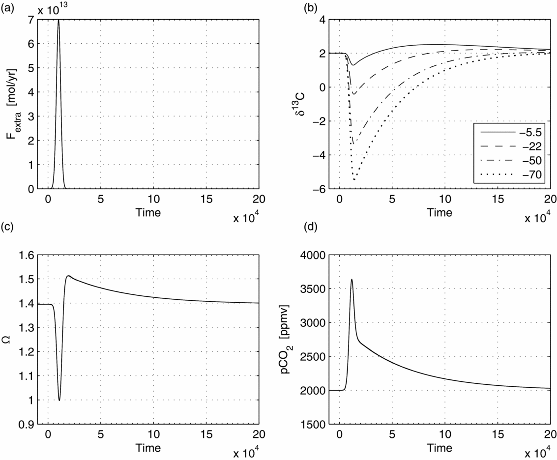
The modelled carbon cycle response to a release of 3.5×10¹⁷ mol of carbon over 20 ka (Fig. 3) is a decline in the δ13C of the ocean (Fig. 3b), a sharp decline followed by a rise in the carbonate saturation state (Ω, Fig. 3c) and a 1.5-fold increase in pCO2 (Fig. 3d), followed by a return to steady state. Assigning more negative δ13C values to the carbon input (Fig. 3b) causes the minimum δ13C values to decline: with an igneous value of −5.5‰ (solid line) the δ13C of seawater decreases from a baseline of 2‰ to a minimum of 1.3‰; with an input of −22‰, corresponding to the input of organic carbon (dashed line), the δ13C of seawater reaches a minimum of −0.4‰; with an input of −50‰, corresponding to thermogenic methane release (dot-dashed line), the δ13C of seawater declines to a minimum of −3.3‰; and with an input of −70‰, corresponding to release of biogenic methane (dotted line), the δ13C of seawater falls to a minimum of −5.5‰. All minima are reached c. 13 ka after the start of the perturbation, which nearly coincides with the peak emission rate at 10 ka. The corresponding decline in saturation state is a result of rapidly increasing oceanic DIC, which reduces the relative abundance of the carbonate ion. A minimum saturation value of 0.99 is reached 11 ka after the perturbation start. Increased calcium concentrations due to increased input from weathering and carbonate dissolution following the CO2 injection lead to a saturation overshoot that peaks at a value of 1.5 c. 18 ka after perturbation start.
Model responses to a single short pulse of carbon simulated by a Gaussian-shaped perturbation with a duration of 20 ka, a total mass of 3.5×10¹⁷ mol, and varying isotopic values. (a) The added carbon flux. (b) δ13C responses for four different carbon isotopic values of the input: solid line −5.5‰; dashed line −22‰; dash-dot line −50‰; and dotted line −70‰. (c) Calcite supersaturation response. (d) pCO2 response. Total run duration is 200 ka.

The pCO2 peak shows two distinct phases characterized by very different slopes. The first is a sharp peak that is driven largely by the volatile emission pulse itself, as is evident by the correspondence between the two curves. During the perturbation, the input of carbon is rapid enough that inputs of alkalinity from carbonate dissolution and silicate weathering are insufficient to counter the increase in pCO2. After the perturbation ends, the input of alkalinity from silicate weathering coupled with burial of carbonate sediments and organic matter drives a gradual reduction in pCO2 back to its pre-excursion baseline. We note that a 20 ka duration for the carbon injection is close to the maximal timescale to effect whole-ocean acidification, as the response time of carbonate dissolution is limited to this timescale by residence time of carbonate in the ocean. The sharp drop in δ13C and carbonate saturation in the model (Fig. 3) indicates that the perturbation is near instantaneous and that releasing carbon on a shorter timescale would make little difference to the modelled response.
3.a.2. 100 ka and 500 ka releases
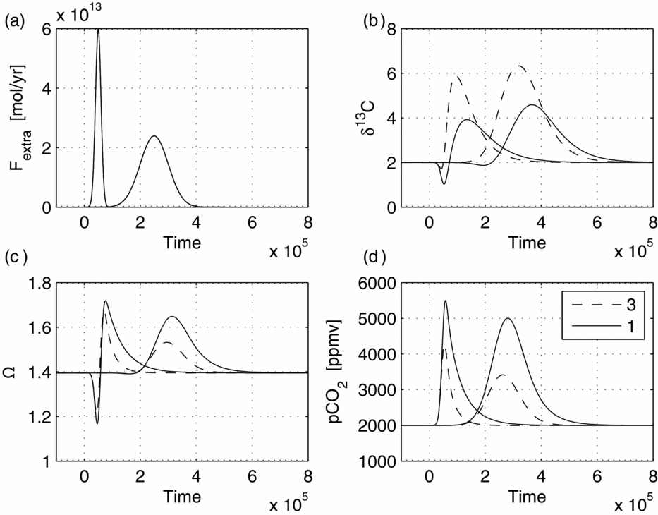
The modelled carbon cycle response to the release of 1.5×10¹⁸ mol of carbon over 100 ka and the release of 3×10¹⁸ mol over 500 ka (both with a δ13C of −5.5‰) are given in Figure 4. The main difference between the 20 ka release (modelled above) and the modelled releases of carbon over hundreds of thousands of years is that the latter drive an increase in pCO2 that is of a sufficiently long duration to stimulate organic carbon burial and effect substantial 13C enrichments. In the first case (1.5×10¹⁸ mol over 100 ka), the rate of carbon emission is still rapid enough that a transient decline in δ13C from 2‰ to 1‰ occurs before the burial of organic carbon increases the δ13C values. In the case of 3×10¹⁸ mol over 500 ka, the decline in δ13C driven by the volatile release is completely offset by the increase in δ13C driven by the increase in organic carbon burial. The magnitude of the resulting 13C enrichment in the two runs is similar (1.9‰ in the 100 ka run versus 2.6‰ in the 500 ka run), indicating that the doubling of the total amount of carbon is approximately offset by the five-fold increase in the duration over which it is released. This numerical result demonstrates that the timescales over which the volcanic degassing occurs have an important impact on 13C enrichment. While shorter pulses are more effective at driving negative δ13C excursions, longer releases are required to drive positive δ13C excursions the longer a release, the more effective it is at driving 13C enrichment.
Model response to a protracted release of carbon. In all panels solid lines are runs with C:P to the first power and dashed lines are runs with C:P to the third power. Increasing the strength of the feedback on organic carbon burial results in an increase in the δ13C response, a decreased response of the carbonate saturation and a decreased response of pCO2. (a) Excess volcanic input from the release of 1.5×10¹⁸ mol of carbon over 100 ka and 3×10¹⁸ released over 500 ka. (b) δ13C responses. (c) Calcite saturation responses. (d) pCO2 responses. Run duration is 800 ka.

In all cases, the positive δ13C excursion lags peak carbon input. In the case of the release of 1.5×10¹⁸ mol over 100 ka, peak δ13C (3.9‰) occurs 78 ka after the maximum rate of carbon emission. In the case of the release of 3×10¹⁸ mol over 500 ka, peak δ13C value (4.6‰) occurs 118 ka after the maximum rate of carbon emission. Similar trends occur in modelled ocean saturation and pCO2. The release of 1.5×10¹⁸ mol over 100 ka drives a transient decline in saturation state (Ω = 1.2) that is closely associated with peak emissions (only 2 ka later), followed by a saturation overshoot (Ω = 1.7) 24 ka after the maximum in the rate of carbon emissions. In all cases pCO2 reaches a maximum in close association with volatile release; in the first case it reaches 4200 ppm only 6 ka after peak volatile release and in the second case it peaks at 3415 ppm 13 ka after peak volatile release.
3.a.3. Sensitivity to anoxia
The inputs and outputs of phosphorus and the degree to which organic carbon burial is decoupled from P outputs are key variables in determining the magnitude and timing of positive excursions in δ13C. Specifically, enhanced remineralization of phosphate is crucial for producing and sustaining positive δ13C excursions because it allows for a decoupling of the burial of phosphate from the burial of alkalinity in a way that weathering inputs cannot. Volcanic activity can lead to increased weathering and input of PO4 3− (either by increasing pCO2 and global weathering or by erupting abundant, highly weatherable basalts), leading to increased organic carbon burial associated with the increased phosphate availability. However, the accompanying increase in the input flux of alkalinity from weathering (which can be thought of as the Ca2+ derived from dissolution of calcium carbonates and calcium silicates) will result in no net change in the fraction of organic carbon burial, and therefore no change in δ13C. For example, a doubling of weathering leading to a doubling of phosphate input will drive a doubling of organic carbon burial. At the same time however, it will double the input of alkalinity and therefore carbonate carbon burial so that, overall, the perturbation to weathering does not lead to any steady-state change in δ13C. The main conclusion is that silicate weathering cannot drive substantial 13C enrichment and that intervals of elevated δ13C require an additional burial-related feedback on phosphate and organic carbon burial. A corollary is that if CO2 drawdown is associated with 13C enrichment, then silicate weathering must be secondary to organic carbon burial in effecting the drawdown.
The theoretical argument for the existence of a burial-related phosphate feedback fits well with the long-standing observation that the burial of phosphate and organic matter can be decoupled via variation in ocean redox conditions. Specifically, phosphate is preferentially released back into the water column in sediments beneath anoxic bottom waters (Ingall, Bustin & Cappellen, Reference Ingall, Bustin and Cappellen1993; van Cappellen & Ingall, Reference van Cappellen and Ingall1994). This mechanism allows large quantities of organic carbon to be buried without simultaneously sequestering the phosphate needed to sustain further productivity or causing immediate and offsetting increases in the inorganic carbon burial flux. Although there are currently no records of P accumulation covering the Late Triassic – Early Jurassic time interval, observations across Mesozoic Ocean Anoxic Events (OAEs) – which share many traits with the Early Jurassic recovery interval (not the least of which are positive δ13C excursions) – show that both the C:P ratio and absolute concentration of P increase in tandem with δ13C (Mort et al. Reference Mort, Adatte, Föllmi, Keller, Steinmann, Matera, Berner and Stüben2007; März et al. Reference März, Poulton, Beckmann, Küster, Wagner and Kasten2008). The anoxia–productivity feedback therefore likely plays a critical role in sustaining the elevated organic carbon burial required for generating positive δ13C excursions.
Certain factors can precondition the ocean towards anoxia and therefore enable the anoxia–productivity feedback to expand and take hold. Elevated temperatures lead to decreased oxygen solubility in the ocean, and certain continental configurations favour nutrient trapping leading to elevated PO4 3− concentrations in certain parts of the ocean (Meyer & Kump, Reference Meyer and Kump2008). A compilation of PO4 3− and H2S concentrations in modern euxinic basins (fjords, the Black Sea) reveals that the two covary and that the linear relation has an intercept (interpreted as the threshold for euxinia) at approximately double the modern deep ocean [PO4 3−] concentrations (Meyer & Kump, Reference Meyer and Kump2008; Ozaki, Tajima & Tajika, Reference Ozaki, Tajima and Tajika2011). A 10× increase in phosphate concentrations leads to pervasive euxinia in a model calibrated to end-Permian conditions (Meyer, Kump & Ridgwell, Reference Meyer, Kump and Ridgwell2008), with peak intensity occurring in oxygen minimum zones which expand substantially. Sea level can also play a role in P cycling through its control on the area of shelf sediments, the chief locus of P and organic carbon deposition. This control is likely to have been amplified during times of extensive euxinia on the continental shelves.
In our modelling effort, we attempt to capture the essence (but obviously not all the details) of the anoxia–productivity feedback (van Cappellen & Ingall, Reference van Cappellen and Ingall1994) by allowing the C:P burial of organic carbon to vary as a function of phosphate output, which is itself first-order dependent on the oceanic mass of phosphate (Table 3). When weathering increases as a result of elevated pCO2, both the modelled inputs and outputs of phosphate increase. The burial of organic carbon also increases, but in a non-linear fashion relative to the phosphate burial flux (Tsandev, Reed & Slomp, Reference Tsandev, Reed and Slomp2012). At steady state, organic carbon burial is tied to P burial via a C:P ratio of 106:1; this ratio however increases when the P burial flux increases, leading to a strong increase in organic carbon burial and therefore δ13C.
To explore the sensitivity of the model to the strength of the parameterized relationship between C:P and P burial, we triple the exponent on the C:P dependence on the phosphate burial so that the relationship becomes cubic instead of linear. Model results under this assumption are given in Figure 4 in dashed lines. Under the larger exponent, the δ13C increase is larger (Fig. 4b) and the increases in carbonate saturation and pCO2 are smaller (Fig. 4c, d) given the same amount of carbon released. This behaviour occurs because the stronger the diversion of the excess volcanic carbon towards organic carbon burial, the smaller the perturbation to the carbonate-silicate sub-cycle, which is the source of the increases in Ω and pCO2. That is, increasing the ‘ease’ with which organic carbon burial occurs per increase in pCO2 means that less change in pCO2 is required to achieve the same level of organic carbon burial and 13C enrichment.
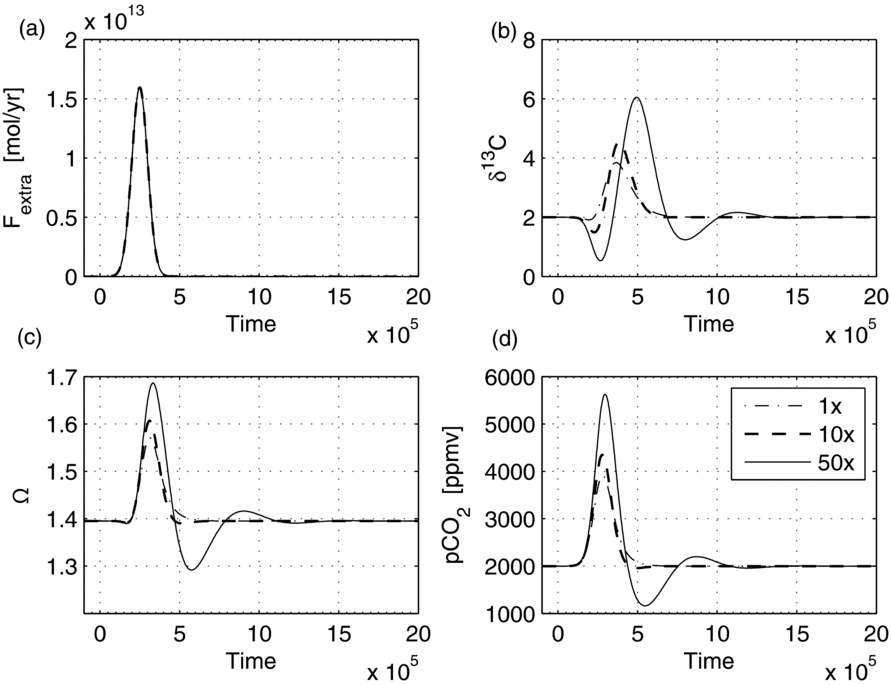
Modifying the starting phosphate concentration in the ocean also increases the magnitude of the δ13C response to perturbation but, less obviously, also leads to a qualitative change in the response of the system (Fig. 5). Increasing the initial phosphate concentration to 10× and 50× leads to damped oscillations that propagate through the entire model, and are expressed in δ13C (Fig. 5b), Ω (Fig. 5c) and pCO2 (Fig. 5d). As we use a variable-step solver tailored for stiff problems (ode15s; Shampine & Reichelt, Reference Shampine and Reichelt1997) the oscillatory outcome is a genuine model response and not an artefact arising from solver instability or round-off accumulation.
Illustration of model sensitivity to initial oceanic PO4 3− concentrations under a scenario of the release of 2×10¹⁸ mol over 500 ka. Dot-dashed line is 1× present oceanic level (0.25 μmol kg−1), dashed line 10× and solid line 50×. Panels as in Figure 4. Increasing the initial phosphate concentration leads to increased residence time for organic carbon burial and results in damped oscillations in the model. The pCO2 response also shows an undershoot which, in the 50× case, is coincident with peak δ13C. Run duration is 2 Ma.

Oscillations occur when the initial phosphate concentration is high because the residence time of phosphate in the model increases as the concentrations increase (from c. 3 ka to 150 ka for the extreme, 50× case). In general, in dynamical systems damped oscillations (complex eigenvalues of the Jacobian) can occur when the relaxation timescales of two state variables are similar, and the derivative of one is inversely dependent on the value of other (Zachos & Kump, Reference Zachos and Kump2005; Pollard, Kump & Zachos, Reference Pollard, Kump and Zachos2013). In our model, the carbon box is dependent on the dynamics of P box through the burial of organic carbon, which is P-dependent, while the behaviour of the P cycle is dependent on pCO2 and hence the content of the carbon box; oscillations therefore occur when the response times of the two boxes become similar.
In this scenario, substantial differences in phase occur between the responses of the different model variables. This phenomenon is most noticeable in the 50× case, where δ13C (Fig. 5b) and pCO2 (Fig. 5d) are of nearly opposite phase. In this scenario, peak carbon input is closely followed by a minimum in δ13C (15 ka later) and a maximum in pCO2 (46 ka later). The subsequent peak in δ13C and minimum in pCO2 lag the peak carbon input substantially (240 ka and 290 ka after peak input, respectively). Moreover, pCO2 declines transiently past its pre-excursion baseline and, due to the lag, coincides with peak δ13C values. Because we do not change the sensitivity of weathering during the model run, this intriguing result indicates that a pCO2 undershoot can occur even without enhanced continental weathering and co-occurs with elevated δ13C.
3.b. Multiple perturbations
Multiple lines of evidence suggest that CAMP eruptions were recurrent, pulsed and relatively brief in nature. Blackburn et al. (Reference Blackburn, Olsen, Bowring, McLean, Kent, Puffer, McHone, Rasbury and Et-Touhami2013) used precise U/Pb radiometric dates from zircons in conjunction with astronomically calibrated cyclostratigraphy (Olsen, Schlische & Fedosh, Reference Olsen, Schlische and Fedosh1996) to constrain the timing of eruption to three main phases: a first major eruptive phase roughly coincident with the main extinction interval (HTQ type basalts: Argana Lower, Intermediate and Upper Basalts in Morocco, North Mountain Basalt in the Fundy Basin and Orange Mountain Basalt in the Newark basin); a second pulse 270 ka later (HFQ/LTQ type basalts: Preakness Basalt in the Newark basin, Hickory Grove basalt in the Culpeper Basin and Holyoke Basalt in the Hartford Basin); and a third pulse 620 ka after the extinction (HFTQ-R: Argana Recurrent Unit and Hook Mountain Basalt).
The isotopic composition of carbonate soil nodules developed in palaeosols from sections containing the CAMP basalt flows in North America indicate that individual CAMP eruptions strongly impacted atmospheric pCO2. The isotopic values indicate that pCO2 increased between two- and three-fold following each of the three major volcanic episodes (given relative to the End Triassic Extinction or ETE) at 0, ETE+270 ka, and ETE+620 ka (Schaller, Wright & Kent, Reference Schaller, Wright and Kent2011; Schaller et al. Reference Schaller, Wright, Kent and Olsen2012). Additionally, a fourth increase in pCO2 at ETE+840 does not coincide with any known volcanic pulses, though it is well within the overall time window for CAMP activity (Knight et al. Reference Knight, Nomade, Renne, Marzoli, Bertrand and Youbi2004; Nomade et al. Reference Nomade, Knight, Beutel, Renne, Verati, Féraud, Marzoli, Youbi and Bertrand2007; Verati et al. Reference Verati, Rapaille, Féraud, Marzoli, Bertrand and Youbi2007; Marzoli et al. Reference Marzoli, Jourdan, Puffer, Cuppone, Tanner, Weems, Bertrand, Cirilli, Bellieni and Min2011). It is important to note that, due to its limited time resolution (hundreds of thousands of years), the proxy likely gives a lower time-averaged bound. The effect of aliasing may have been particularly important during the few hundred years immediately following each eruption, when pCO2 may have been substantially higher than indicated by the proxy. The falloff from peak pCO2 values is observed to occur on timescales of hundreds of thousands of years which Schaller, Wright & Kent (Reference Schaller, Wright and Kent2011) and Schaller et al. (Reference Schaller, Wright, Kent and Olsen2012) interpret to result from silicate weathering. However, c. 90% of the decline in pCO2 following a carbon pulse occurs within the first 10 ka when carbon dioxide is absorbed by the ocean and removed by carbonate dissolution (Archer, Kheshgi & Reimer, Reference Archer, Kheshgi and Reimer1997; Rampino & Caldeira, Reference Rampino and Caldeira2011). Only the remaining 10% of the excess pCO2 is removed by silicate weathering on timescales of hundreds of thousands of years. We therefore suggest that the protracted e-folding times of CO2 drawdown indicated by the palaeosol proxy are best interpreted to reflect waning degassing from the basalt flows and/or protracted thermogenic CO2 devolatilization from intruded sediments, rather than extremely slow continental weathering following near-instantaneous pulses. In other words, intervals of elevated pCO2 lasting hundreds of thousands of years likely require sustained carbon input on those same timescales.
Lastly, the δ13C decline immediately below the oldest basalts in Morocco (Deenen et al. Reference Deenen, Ruhl, Bonis, Krijgsman, Kuerschner, Reitsma and van Bergen2010; Dal Corso et al. Reference Dal Corso, Marzoli, Tateo, Jenkyns, Bertrand, Youbi, Mahmoudi, Font, Buratti and Cirilli2014) indicates an earlier injection of 13C-depleted carbon that preceded the eruption of the first basalts, perhaps by as little as 10–20 ka. Specifically, if the Talcott and Orange Mountain Basalts (above which the palaeosol proxy indicates that pCO2 levels increased) are younger than the Argana basalt, which is underlain by sediments whose δ13C values are already decreasing, then an additional pulse of 13C-depleted carbon predating the basalts is required to accommodate the declining δ13C values, even in the absence of an indication for an additional pCO2 pulse in the North American palaeosol record. The decline in δ13C below the basalts in Morocco is unlikely to be a result of contact metamorphism from the basalts above, as metamorphic devolatilization would drive off labile components which tend to be 13C-depleted (Hayes, Kaplan & Wedeking, Reference Hayes, Kaplan, Wedeking and Schopf1983), leading to more elevated δ13C values in the residuum. The evidence therefore supports a total of five carbon pulses: an initial short (<20 ka) pulse of highly 13C-depleted carbon, and the four releases identified by the pCO2 palaeosol proxy (of which the first three correspond to known CAMP flows) which we postulate had a volcanic δ13C signature. A scenario in which the first pulse of carbon was related to devolatilization associated with intrusion of CAMP basalts into coals or organic-rich sedimentary basins (perhaps associated with establishment of the volcanic plumbing), while the other pulses were mostly associated with degassing of the basalt flows themselves, could account nicely for our postulated heterogeneity in the δ13C of the emitted volatiles.
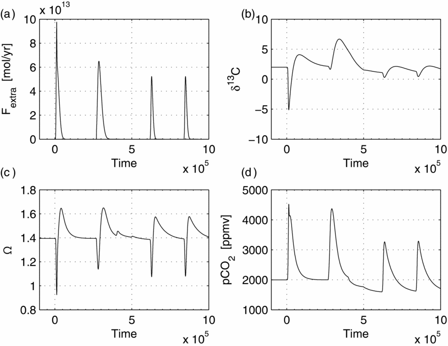
Assuming a linear relationship between the volcanic forcing and the δ13C response (as in Fig. 4, as opposed to Fig. 5), it is possible to apply five perturbations to the model with a spacing suggested by the chronology above and to tune model and perturbation parameters to the observed δ13C record (Fig. 6). With the timing of the perturbations constrained, there are still three degrees of freedom left: the duration of the volatile release; the amount of degassed carbon; and its isotopic composition. We describe our choices with respect to the negative N1 excursion (−5‰), the positive P1 excursion (+4‰) and the large protracted P2 excursion (+6‰).
Model output under a multi-perturbation scenario. A pulse of highly depleted carbon (−70‰) with a more 13C enriched tail (−5.5‰) is used to model the first negative–positive couplet corresponding to the N1 and P1 δ13C excursions. A second more protracted pulse of volcanic carbon (−5.5‰) is used to drive the protracted second positive excursion (P2). A 17% increase in silicate weathering is initiated at 400 ka to drive a decline in baseline δ13C. The anoxia sensitivity is further lowered from 3 to 1 power at 500 ka to achieve a more muted effect of the last two carbon pulses on δ13C. Total run duration is 1 Ma. Panels as in Figure 4.

The negative N1 excursion can be readily produced in the model, while simultaneously reproducing the observed doubling of pCO2 from 2000 ppm to 4000 ppm by assuming a 20 ka Gaussian-shaped pulse of 3.5×10¹⁷ mol of CO2 with an isotopic value of −70‰. This value is similar to that calculated by Ruhl et al. (Reference Ruhl, Bonis, Reichart, Damsté and Kürschner2011). The duration (20 ka) of the pulse of carbon is sufficiently short to drive a drop in the saturation state of the ocean in conjunction with the drop in δ13C.
Replicating the subsequent positive excursion (P1, +4‰) within our model requires a more complex emission scenario. The model indicates that the organic carbon burial generated by a single methane release is too small to drive a +4‰ excursion (Figs 3, 6), and that additional carbon input is required. However, a single pulse of 3.5×10¹⁷ mol C over 60 ka (the inferred maximal duration of the HTQ basalts) is insufficient to drive such a positive excursion, even assuming complete return to a 2‰ baseline following the release of the methane (c. 200 ka), a relatively enriched value (−5.5‰) of the emitted carbon and a strong (cubed power) feedback on organic carbon burial. We find that a Gaussian pulse of 1.2×10¹⁸ mol of CO2 released over 60 ka, starting when methane peaks, produces the patterns of changes observed in the δ13C and pCO2 proxy records. We further set the Gaussian to be strongly left-skewed so that the combined shape of the two perturbations (methane and CO2) is a spike that descends smoothly into a protracted right tail. The reason that we chose this particular parameterization is that, although two symmetric Gaussian pulses lead to identical effects on δ13C as the single composite, the two pulses lead to two resolvable peaks in pCO2 and Ω, phenomena for which we currently lack evidence. Following the methane pulse by a more protracted flux of volcanic carbon leads to a rapid recovery and an increase in δ13C, so that a small positive δ13C excursion results.
Replicating the large (+6‰) P2 excursion requires an order of magnitude more carbon. To simultaneously honour the carbon isotope record and the pCO2 constraints, this carbon must be released over a longer timescale. We find that the asymmetric release of 2×10¹⁸ mol over 150 ka (the inferred duration of the LTQ/HFQ basalts) can account for both observations quite well. In the model, 3.9-fold and 4.1-fold increases in organic carbon burial are associated with the P1 and P2 positive δ13C excursions, but both excursions are associated with only a 1.6-fold increase in carbonate carbon burial. In absolute terms, peak carbon removal rates are 23 Tmol a−1 (1 Tmol = 1012 mol) via carbonate burial but 35 Tmol a−1 and 39 Tmol a−1 via organic carbon burial. Since carbonate carbon burial represents the sum of carbonate and silicate weathering, the greater burial of organic carbon (necessary to drive up δ13C values) indicates that the decline in pCO2 following the first two peaks is more strongly driven by organic carbon burial than by silicate weathering.
We set the fourth and fifth volatile releases (at ETE+620 and ETE+840 ka) to 7.5×10¹⁷ of CO2 at −5.5‰ over 100 ka each in an effort to account for the 1–2‰ positive excursions and the approximate doubling of pCO2 that are observed. Introducing a larger amount of carbon in each pulse results in a larger pCO2 peak (closer to the observed proxy values), but also produces larger δ13C excursions as well as larger drops in carbonate saturation, predictions which are inconsistent with the geologic evidence. Even with these ‘compromise’ values, we find that a lowering of the anoxia sensitivity in the model is required from cubic (power of 3) to linear (power of 1) to achieve the apparently much muted impact of these pulses on δ13C. If the original sensitivity is instead maintained, the resulting positive excursions are closer to 2‰ than 1‰ in magnitude.
The final perturbation required to account for the isotopic record in the Lombardy Basin is an additional carbonate sink. In the Lombardy Basin, the δ13C record stabilizes at a value close to 1‰ following the P2 excursion, c. 1‰ lower than the 2‰ baseline typical of the uppermost Triassic. A similar trend occurs in the Queen Charlotte Islands (Williford et al. Reference Williford, Ward, Garrison and Buick2007), indicating that it is likely a global phenomenon. If so, this shift in baseline requires an increase in the delivery of alkalinity from weathering relative to carbon from volcanism. In our model, we find that increasing weathering by 17% (2×10¹⁸ mol increase from the 12×1018 mol a−1 baseline) beginning at 500 ka, together with the decrease in the anoxia exponent and approximately in line with the peak of the P2 excursion, can account for the decline in δ13C baseline values. This increase in weathering in the model triggers a decrease in pCO2, as well as a decline in organic carbon burial. The 17% increase in weathering we apply is comparable to, though smaller than, the 1.5× to 2× increase calculated by Schaller et al. (Reference Schaller, Wright, Kent and Olsen2012) using the model of Bergman, Lenton & Watson (Reference Bergman, Lenton and Watson2004). In this scenario (shift in baseline δ13C), in contrast to the CO2 drawdown associated with positive excursions, the increased delivery of alkalinity from carbonate and silicate weathering are the predominant factors in the CO2 drawdown. It is attractive to speculate that this model result corresponds to an increase in the delivery of alkalinity from fresh CAMP basalts that were erupted in the tropics, where high temperatures and abundant rainfall contributed to vigorous chemical attack and rapid mineral dissolution. Lastly, although we describe the model outputs in terms of the δ13C of carbonates, incorporating a variable CO2 and PO4 3−-dependent fractionation (Kump & Arthur, Reference Kump and Arthur1999) makes no significant difference in the model output. The δ13C of organic carbon faithfully tracks the values of the carbonate carbon δ13C as the response is very nearly saturated at the high-baseline pCO2 (2000 ppm). At this pCO2 the initial fractionation is already very near the maximal possible expressed fractionation.
4. Discussion
The key features of the carbon isotopic record of the Triassic–Jurassic transition are the N1, P1 and P2 excursions (Figs 1, 7, 8), which are known from globally distributed sections. The ‘initial’ N1 negative δ13C excursion, which co-occurs with the end-Triassic extinction, is one of the most widely observed features of the T–J carbon isotopic record (Hallam & Goodfellow, Reference Hallam and Goodfellow1990; Hallam, Reference Hallam1994; Morante & Hallam, Reference Morante and Hallam1996; McRoberts, Furrer & Jones, Reference McRoberts, Furrer and Jones1997; Pálfy et al. Reference Pálfy, Demény, Haas, Hetényi, Orchard and Veto2001; Hesselbo et al. Reference Hesselbo, Robinson, Surlyk and Piasecki2002; Guex et al. Reference Guex, Bartolini, Atudorei and Taylor2004; Galli et al. Reference Galli, Jadoul, Bernasconi and Weissert2005; Ward et al. Reference Ward, Garrison, Williford, Kring, Goodwin, Beattie and McRoberts2007; Ruhl, Kürschner & Krystyn, Reference Ruhl, Kürschner and Krystyn2009; Clémence et al. Reference Clémence, Bartolini, Gardin, Paris, Beaumont and Page2010; Deenen et al. Reference Deenen, Ruhl, Bonis, Krijgsman, Kuerschner, Reitsma and van Bergen2010; Ruhl, Veld & Kürschner, Reference Ruhl, Deenen, Abels, Bonis, Krijgsman and Kürschner2010; Črne et al. 2011; Ruhl et al. Reference Ruhl, Bonis, Reichart, Damsté and Kürschner2011; Bachan et al. Reference Bachan, de Schootbrugge, Fiebig, McRoberts, Ciarapica and Payne2012; Lindström et al. Reference Lindström, de Schootbrugge, Dybkjær, Pedersen, Fiebig, Nielsen and Richoz2012; Dal Corso et al. Reference Dal Corso, Marzoli, Tateo, Jenkyns, Bertrand, Youbi, Mahmoudi, Font, Buratti and Cirilli2014). It has even been proposed as a chemostratigraphic marker for the stage boundary (McRoberts, Ward & Hesselbo, Reference McRoberts, Ward and Hesselbo2007). Although its timing is increasingly well constrained (Schaltegger et al. Reference Schaltegger, Guex, Bartolini, Schoene and Ovtcharova2008; Schoene et al. Reference Schoene, Guex, Bartolini, Schaltegger and Blackburn2010), uncertainty remains with respect to its magnitude as recorded in organic and carbonate carbon (see Greene et al. Reference Greene, Martindale, Ritterbush, Bottjer, Corsetti and Berelson2012 and Bachan, van de Schootbrugge & Payne, 2014 for discussion). Nevertheless, that a coincidence of extinction, acidification and a negative δ13C excursion is the null expectation under a carbon-release scenario (Fig. 3) is a strong argument in favour of a primary exogenic origin for the N1 excursion. Our modelling joins previous work (Beerling & Berner, Reference Beerling and Berner2002; Berner & Beerling, Reference Berner and Beerling2007; Paris et al. Reference Paris, Donnadieu, Beaumont, Fluteau and Goddéris2012) in supporting the notion that rapid release of large amounts of 13C-depleted carbon can account for both the negative δ13C excursion and a drop in the carbonate saturation state associated with the extinction.
Additionally, our modelling highlights a required association between the negative carbon-isotope excursion and subsequent burial of organic carbon such that a speedy ‘bounce-back’ in δ13C resulted. The duration of the recovery from a release of light carbon, if only by dilution, is between 100 and 500 ka (Fig. 3; Beerling & Berner, Reference Beerling and Berner2002). Assuming that the negative δ13C excursion represents such a protracted time interval requires that a substantial portion of Hettangian time be concentrated in 1 m of marl in the Lombardy Basin, Italy, while the rest of it is represented by over 600 m of sediment; it also requires that in St Audrie's Bay, UK, up to 500 ka is represented in 50 cm of sediment of the Lilstock Formation, while the entire Hettangian above (c. 2 Ma) is represented by 70 m of Blue Lias Formation (Ruhl et al. Reference Ruhl, Deenen, Abels, Bonis, Krijgsman and Kürschner2010). In Austria, we find it equally unlikely that so much time would be concentrated in less than 20 cm of strata in the Eiberg Basin in what are otherwise expanded sections (Ruhl, Kürschner & Krystyn, Reference Ruhl, Kürschner and Krystyn2009). Furthermore, the N1 negative excursion in the Lombardy Basin is observed to be completely contained within the extinction-marl (Bachan, van de Schootbrugge & Payne, Reference Bachan, de Schootbrugge and Payne2014). If the extinction-marl is acidification-induced (Hautmann, Reference Hautmann2004), its duration, and therefore that of the excursion, cannot be longer than a few thousand years, which is the response time of the carbonate system in the ocean (Broecker, Reference Broecker1971). It is therefore probable that substantial amounts of organic carbon were buried immediately following the injection of the 13C-depleted carbon such that the isotopic values rebounded quickly.
Consistent with the supposition that organic carbon burial immediately followed carbon introduction, a small (2‰) positive excursion occurs immediately above the N1 negative excursion near the base of the Planorbis zone (the P1 excursion). In the UK, this carbon isotope excursion is very well characterized in both carbonate carbon and organic carbon in Lyme Regis, Lavernock Point and Doniford sections (Korte et al. Reference Korte, Hesselbo, Jenkyns, Rickaby and Spötl2009; Clémence et al. Reference Clémence, Bartolini, Gardin, Paris, Beaumont and Page2010). In both the Lombardy Basin, southern Alps, Italy (Bachan et al. Reference Bachan, de Schootbrugge, Fiebig, McRoberts, Ciarapica and Payne2012) and New York Canyon, Nevada, USA (Bartolini et al. Reference Bartolini, Guex, Spangenberg, Schoene, Taylor and Schaltegger2012), the P1 excursion is distinctly recognizable (Figs 1, 7). It is followed by the much larger positive P2 excursion (up to +6‰) recorded in Kennecott Point, Queen Charlotte Islands, British Columbia (Williford et al. Reference Williford, Ward, Garrison and Buick2007), New York Canyon, Nevada, USA (Bartolini et al. Reference Bartolini, Guex, Spangenberg, Schoene, Taylor and Schaltegger2012) and the Lombardy Basin, southern Alps, Italy (Bachan et al. Reference Bachan, de Schootbrugge, Fiebig, McRoberts, Ciarapica and Payne2012).
The positive δ13C excursions are likely global and synchronous. In the Lombardy Basin the 13C enrichment associated with P2 excursion occurs in both carbonate and organic carbon from the same samples (Bachan et al. Reference Bachan, de Schootbrugge, Fiebig, McRoberts, Ciarapica and Payne2012), a robust indication that it was already present in the original water column and is not diagenetic. The occurrence of the P2 excursion in both δ13Corg and δ13Ccarb further discounts a compositional control on δ13C (van de Schootbrugge et al. Reference van de Schootbrugge, Payne, Tomasovych, Pross, Fiebig, Benbrahim, Föllmi and Quan2008). In addition, the P2 excursion also occurs in organic carbon from extra-Tethyan sections in British Columbia and Nevada. The P2 excursion is not apparent in the δ13C of bulk organic carbon in the Newark basin (Whiteside et al. Reference Whiteside, Olsen, Eglinton, Brookfield and Sambrotto2010) and only occurs in muted form in Saint Audrie's Bay (Ruhl et al. Reference Ruhl, Deenen, Abels, Bonis, Krijgsman and Kürschner2010; Hüsing et al. Reference Hüsing, Beniest, van der Boon, Abels, Deenen, Ruhl and Krijgsman2014). In both sections small-scale variability is much more prominent than any long-term trend; in Saint Audrie's Bay over 2‰ of bed-to-bed variability occurs, while in the Newark basin it is closer to 7‰ so that intense local C-cycling may have masked the expression of global δ13C trends.
A few broader considerations are pertinent to the question of synchroneity of the positive excursions. An increase in the δ13C of the ocean–atmosphere pool will result from increased organic carbon burial irrespective of where it occurs: it can be localized and intense or extra-regional and diffuse. Nonetheless, in places where the rate of carbon export from the surface waters exceeds the rate at which the waters are mixed, local 13C enrichment can arise without an accompanying increase in organic carbon burial. Some variation in the magnitude of the P2 excursion is apparent, suggesting the existence of regional carbon-isotopic gradients: the P2 excursion reaches +6‰ in northern Italy while reaching only +4‰ in southern Italy (Bachan et al. Reference Bachan, de Schootbrugge, Fiebig, McRoberts, Ciarapica and Payne2012). It is, however, not possible to explain the entire magnitude of the excursion in this way. The burial of 13C-enriched carbonates in one locality (without corresponding burial of organic carbon) must lead to a reduction in the δ13C of carbonates deposited elsewhere due to the constraints imposed by mass balance. In fact, the reason that local deviations from the global δ13C record can exist (e.g. Swart, Reference Swart2008) is precisely because they are local, and therefore have little leverage on the global carbon cycle. A positive δ13C excursion can be local, but it cannot be both ‘local’ and widespread at the same time without incurring carbon cycle imbalances.
A historical perspective is also valuable. The question of whether positive carbon-isotope excursions represent synchronous chronostratigraphic markers has played out numerous times (the Cenomanian–Turonian boundary is a notable early example; Scholle & Arthur, Reference Scholle and Arthur1980; Bralower, Reference Bralower1988). The debate has so far been consistently resolved in favour of the δ13C values being synchronous and the biostratigraphy diachronous. While this is no guarantee that the T–J boundary δ13C record follows the same trend, it does offer a strong expectation that it should.
The observed enrichment in 13C indicating elevated levels of organic carbon burial following the end-Triassic extinction is also consistent with long-standing observations that the earliest Jurassic was a period of widespread anoxia and deposition of organic-rich sediments (Hallam, Reference Hallam1995). For instance, the Hettangian-aged Blue Lias Formation in the UK has TOC levels in the range of 1–10% for the majority of the section, even exceeding 10% in some horizons (Ruhl et al. Reference Ruhl, Deenen, Abels, Bonis, Krijgsman and Kürschner2010). In the Lombardy Basin, the beds immediately above the extinction marl (belonging to the Malanotte Formation) are relatively TOC-rich dark-coloured finely bedded micrites and shales (Galli et al. Reference Galli, Jadoul, Bernasconi, Cirilli and Weissert2007; Bachan et al. Reference Bachan, de Schootbrugge, Fiebig, McRoberts, Ciarapica and Payne2012). Nevertheless, studies of organic carbon burial in modern marine environments (Berner, Reference Berner1982) indicate that the bulk of organic carbon burial occurs in shelf environments and near river deltas, where abundant clays are present for rapid burial of adsorbed organic carbon and short oxygen exposure times minimize remineralization (Hartnett et al. Reference Hartnett, Keil, Hedges and Devol1998). In these environments, organic carbon is not highly concentrated. Thus, even though black shales are indicative of anoxia and locally high productivity, they do not necessarily constitute an avenue of significant organic carbon burial. Consequently, though cases of correspondence between the geochemical evidence and sedimentological observations are reassuring, the widespread preservation of black shales is not required to demonstrate elevated rates of organic carbon burial. Our modelling, based on the δ13C record, offers a quantitative estimate of the increase in organic carbon burial which was required to produce the positive excursions: in our multi-perturbation modelling scenario 3.9- and 4.3-fold increases in organic carbon burial are required to produce the P1 and P2 excursions, respectively.
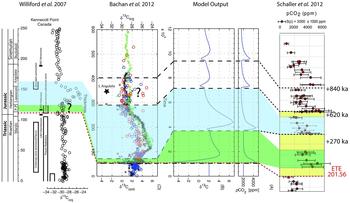
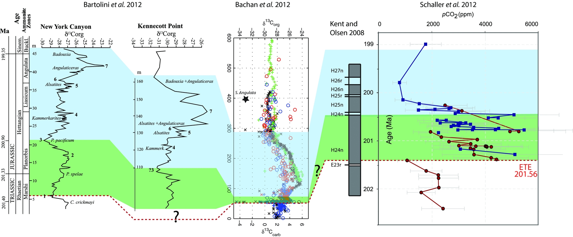
Although the magnitude of the P2 positive δ13C excursion is increasingly well-constrained, its timing during the Hettangian period remains incompletely understood. Careful consideration of the available biostratigraphic and radiometric constraints reveals that there are currently two possible (and conflicting) age assignments for the P2 positive excursion, with very different implications for its impacts on ocean–atmosphere chemistry. The first assignment is an early–middle Hettangian (Planorbis–Liassicum) age, while the other is a middle–late Hettangian (Liassicum–Angulata) age. The first age assignment is based on the biostratigraphy and isotopic observations from Kennecott Point, Queen Charlotte Islands, British Columbia (Carter & Hori, Reference Carter and Hori2005; Ward et al. Reference Ward, Garrison, Haggart, Kring and Beattie2004; Longridge et al. Reference Longridge, Carter, Haggart and Smith2007a , Reference Longridge, Carter, Smith and Tipper b , Reference Longridge, Palfy, Smith and Tipper2008; Williford et al. Reference Williford, Ward, Garrison and Buick2007) and from the Lombardy Basin, Italy (Kronecker, Reference Kronecker1910; Gaetani, Reference Gaetani1970; Galli et al. Reference Galli, Jadoul, Bernasconi, Cirilli and Weissert2007; Jadoul & Galli, Reference Jadoul and Galli2008; van de Schootbrugge et al. Reference van de Schootbrugge, Payne, Tomasovych, Pross, Fiebig, Benbrahim, Föllmi and Quan2008; Bachan et al. Reference Bachan, de Schootbrugge, Fiebig, McRoberts, Ciarapica and Payne2012). In both these sections, the excursion extends from near the Triassic–Jurassic boundary to well below the Hettangian–Sinemurian boundary (Fig. 7). In contrast with the above age assignments (early–middle Hettangian), Bartolini et al. (Reference Bartolini, Guex, Spangenberg, Schoene, Taylor and Schaltegger2012) assign a late Hettangian (Angulata Zone) age for the P2 excursion, based on the observation that in New York Canyon, Nevada, the excursion is situated within Angulata-aged beds. Bartolini et al. (Reference Bartolini, Guex, Spangenberg, Schoene, Taylor and Schaltegger2012) also point out that a large positive excursion of the same age occurs in low-resolution data in Lyme Regis, UK, found in the supporting material of Whiteside et al. (Reference Whiteside, Olsen, Eglinton, Brookfield and Sambrotto2010). They further reinterpret the stratigraphy of Longridge et al. (Reference Longridge, Palfy, Smith and Tipper2008) for Kennecott Point so that a late Hettangian age is also obtained there for the excursion. However, this reinterpretation implies that the boundary was previously grossly misplaced there (Fig. 8). Available radiometric ages highlight the difficulty in reconciling the two age assignments. The most recent radiometric age for the end-Triassic extinction is 201.564±0.015 Ma (Blackburn et al. Reference Blackburn, Olsen, Bowring, McLean, Kent, Puffer, McHone, Rasbury and Et-Touhami2013), a small change from the 201.58±0.28 Ma obtained by Schaltegger et al. (Reference Schaltegger, Guex, Bartolini, Schoene and Ovtcharova2008) and 201.31±0.43 Ma of Schoene et al. (Reference Schoene, Guex, Bartolini, Schaltegger and Blackburn2010), suggesting convergence in its absolute age. An age of 199.43±10 Ma for the Hettangian–Sinemurian boundary was obtained by Guex et al. (Reference Guex, Schoene, Bartolini, Spangenberg, Schaltegger, O’Dogherty, Taylor, Bucher and Atudorei2012) from an ash bed in Badouxia-canadensis-containing beds in Peru, close to the Hettangian–Sinemurian boundary (updated from an age of 199.53±0.29 Ma obtained by Schaltegger et al. Reference Schaltegger, Guex, Bartolini, Schoene and Ovtcharova2008). These data indicate a c. 2 Ma duration for the Hettangian period. Interpolating between the tie-points suggests that either the P2 excursion spanned slightly less than the first half of the Hettangian age (Planorbis–Liassicum zones) and that significant time passed between its decline and the base of the Sinemurian (perhaps the entire Angulata zone, up to 1 Ma), or that it began c. 1 Ma into the Hettangian age and peaked near its end. The two age assignments for the P2 excursion are therefore mutually exclusive.
Stratigraphic correlations and implications for carbon cycle dynamics if the P2 positive δ13C excursion is of early–middle Hettangian in age. Under this scheme the P1 and P2 excursions are associated with individual pulses of CAMP volatiles and peaks in pCO2.

Correlations and implications for carbon cycle dynamics if the P2 excursion (excursion 7 of Bartolini et al. Reference Bartolini, Guex, Spangenberg, Schoene, Taylor and Schaltegger2012) is late Hettangian in age (compare with Figure 7). Under this scheme the P1 excursion (excursion 2 of Bartolini et al. Reference Bartolini, Guex, Spangenberg, Schoene, Taylor and Schaltegger2012) is correlative with the entire interval of pCO2 perturbations. The P2 positive excursion is then coincident with the pCO2 undershoot (see Fig. 5). Note that this interpretation implies that the boundary has been previously misplaced at Kennecott Point.

Because the record of CAMP pulses in Morocco and North America are all dated to within 1 Ma of the extinction and do not extend past the first half of the Hettangian period (the last CAMP basalt in North America is dated at ETE+620 ka, which is at 200.9 Ma; Blackburn et al. Reference Blackburn, Olsen, Bowring, McLean, Kent, Puffer, McHone, Rasbury and Et-Touhami2013), an early Hettangian age for the excursion would suggest synchroneity with the volcanism in the Newark basin and elsewhere (Fig. 7). If, on the other hand, the P2 carbon isotope excursion is late Hettangian in age, then even the last of the volatile pulses (at ETE+840 ka) could not have corresponded with it. In that case, the isotope excursion would be coincident with the cooling and pCO2 undershoot identified by Schaller et al. (Reference Schaller, Wright, Kent and Olsen2012) (Fig. 8). Hence, in the first option the P1 and P2 positive excursions are associated with warming and pCO2 peaks (Fig. 7), whereas in the second option the P2 excursion is associated with cooling, pCO2 drawdown and even undershoot (Fig. 8).
If the first correlation is correct, then our multiple-perturbation modelling run (Fig. 6) offers a carbon cycle scenario that honours both the pCO2 and δ13C constraints (Fig. 7). The perturbation scheme comprises 5 pulses of carbon: the first is highly 13C-depleted pulse (−70‰) which corresponds to the N1 negative δ13C excursion. It grades smoothly into a second volcanic carbon emission (−5‰) which corresponds to the P1 excursion and the third pulse corresponds to the P2 excursion. The last two pulses have very muted effects on δ13C and correspond to CO2 drawdown (putatively due to increased delivery of alkalinity from CAMP volcanic rocks).
If, however, the latter correlation is correct (Fig. 8), then our model runs in which damped oscillations occur offer a potential explanation (Fig. 5). In those runs, the pCO2 minimum coincides with peak δ13C values so that they are of nearly opposite phase and, most importantly, substantially lag the carbon input pulse. In this scenario, the pCO2 drawdown recognized in the palaeosol proxy record would have been driven by enhanced organic carbon burial, rather than due to increased weathering of CAMP basalts. Intriguingly, under this correlation the complex carbon cycle behaviour would be entirely due to internal dynamics and would be triggered by (but not driven by) the perturbations associated with CAMP volcanism.
If the latter correlation is correct, a key question arises: if the P2 positive excursion occurs well after the volcanic carbon pulses have finished, why then does the δ13C record only show a single positive δ13C excursion in the Planorbis zone (the P1 excursion) and no hint of multiple pulses (Fig. 8)? The total duration of the four pCO2 pulses (nearly 1 Ma) is much longer than the residence time of carbon in the ocean–atmosphere system, implying that the pulses should be individually distinguishable in their effects on the global carbon cycle and δ13C. A complete failure of the (global) carbon isotope record to record the four individual pulses of carbon or their aliasing somehow into a single positive δ13C excursion (the P1 excursion) – on top of the special consideration (elevated P concentrations) required to explain the lag between the carbon pulses and the P2 excursion – would constitute a substantial challenge to our understanding of carbon cycle dynamics.
The key to further progress is distinguishing between these very different carbon cycle scenarios by improving the age constraints on the P2 excursion. At least one prediction that can be offered is that if the P2 excursion is late Hettangian as opposed to early Hettangian in age, the geomagnetic polarity reversals correlative to H24R–H27N (Kent & Olsen, Reference Kent and Olsen2008; Muttoni et al. Reference Muttoni, Kent, Jadoul, Olsen, Rigo, Galli and Nicora2010) should occur in the Albenza Formation (as opposed to the Sedrina Limestone) in the Lombardy Basin, Italy and in the Sunrise Formation in New York Canyon, Nevada.
5. Conclusions
Consistent with previous studies (Beerling & Berner, Reference Beerling and Berner2002; Berner & Beerling, Reference Berner and Beerling2007; Paris et al. Reference Paris, Donnadieu, Beaumont, Fluteau and Goddéris2012), our modelling of Triassic–Jurassic carbon cycle dynamics suggests that the rapid input of highly 13C-depleted carbon (−70‰) can explain the negative excursion in δ13C and increase in atmospheric pCO2 associated with the end-Triassic mass extinction (Fig. 3). Such a scenario can also account for ocean acidification, consistent with selective extinction of heavily calcified marine invertebrate animals (Kiessling & Simpson, Reference Kiessling and Simpson2011) and lithological evidence for a carbonate dissolution event (Hautmann, Reference Hautmann2004). However, our model further indicates that rapid rebound from the most negative carbon isotope values requires that burial of substantial amounts of organic carbon quickly followed the carbon injection. Such rapid organic carbon burial likely occurred primarily on the continental shelves where expansion of existing oxygen minimum zones would have been most rapid (on the order of thousands to tens of thousands of years).
Our modelling also indicates that volcanic carbon pulses of sufficient duration and magnitude can give rise to positive δ13C excursions through acceleration of organic carbon burial (Fig. 4). However, when the phosphorus residence time in the model is increased damped oscillations occur, indicating that a more complex carbon cycle response to a single disturbance is possible (Fig. 5). In the first case, there is a tight coupling between elevated δ13C and CO2 input and the increased δ13C is associated with declining (but still elevated) pCO2 (Fig. 4), whereas in the second case the elevated δ13C is in opposite phase to pCO2 and lags the carbon input substantially (Fig. 5).
Uncertainty regarding the timing during the Hettangian period of peak δ13C values (the P2 excursion) leaves open two possibilities corresponding to the two different carbon cycle scenarios. The first option is that the P2 positive excursion is of early–middle Hettangian age, which implies that it coincided with CAMP-related volcanic pulses. In this case a multi-pulse model scenario can be fitted to the isotopic record (Fig. 6) and the P1 and P2 excursions correspond directly to pulses of carbon from CAMP volcanics (Fig. 7). The second option is that the P2 excursion is of a middle–late Hettangian age, in which case it lagged the CAMP volatile pulses substantially, and was associated with pCO2 drawdown and perhaps even undershoot (Fig. 8). Our model runs in which damped oscillations occur offer a potential carbon-cycle-based explanation for this observation. If the former scenario is correct, then the δ13C perturbations did not extend past 500 ka after the extinction, and the biotic recovery was under way even as the final two pulses of CAMP volcanism (at ETE+620 ka and ETE+840 ka) were occurring. However, if the latter scenario is correct, then carbon cycle instability persisted for up to a million years past the cessation of pulsed CAMP activity, and stabilization was only achieved at the beginning of the Sinemurian period. The protracted delay between the physical forcing and biotic response in the latter case implicates ocean biogeochemical dynamics as the cause for the delayed recovery and carbon cycle instability. Improving the geochronological constraints on the P2 excursion will help determine whether the recovery from the end-Triassic mass extinction was delayed by internal dynamics of the exogenic carbon cycle or repeated external perturbations.
Acknowledgements
The authors thank the editor (P. Wignall) and an anonymous reviewer for comments which greatly improved this manuscript. AB gratefully acknowledges support from a National Science Foundation Graduate Research Fellowship.
Supplementary material
To view supplementary material for this article, please visit http://dx.doi.org/10.1017/S0016756815000126.