




No CrossRef data available.
LIKELIHOOD RATIO ORDERING OF THE INSPECTION PARADOX
Published online by Cambridge University Press: 01 October 2004
Abstract
In this article, some results on stochastic comparisons of the inspection paradox introduced by Ross [Probability in the Engineering and Informational Sciences 17: 47–51 (2003)] are established in the sense of the likelihood ratio order.
Information
- Type
- Research Article
- Information
- Probability in the Engineering and Informational Sciences , Volume 18 , Issue 4 , October 2004 , pp. 503 - 510
- Copyright
- © 2004 Cambridge University Press
1. INTRODUCTION AND THE MAIN RESULTS
Ross [3] introduced the following interesting inspection paradox. Consider a total of n families, each having children who attend a certain school. Let Xi denote the number of children of family i, i = 1,…,n, and assume that the Xi are independent and identically distributed (i.i.d.) with probability mass function

, and finite mean μ. Now, one of the school children is randomly chosen, and let I denote the number of the family to which the selected child belongs. (Sometimes, we use In to emphasize the number of the families.) Ross [3] proved that for X1 ≤lr XI,

and

The formal definitions of the order ≤lr and of the other stochastic orders are given in Definition 1.1.
The purpose of this article is to investigate some results on stochastic comparisons of the above inspection paradox in the sense of the likelihood ratio order. More precisely, we establish the following theorems.
Theorem 1.1: If X ≥lr Y, then XI ≥lr YI.
Theorem 1.2: For

.
Theorem 1.3: If X is PF2 (Pólya frequency of order 2) (i.e., X has a logconcave mass function), then XI is PF2.
The proofs of Theorems 1.1–1.3, as well as some remarks, are given in Section 2.
Finally, some stochastic orders that will be used in this note are recalled in the following definition.
Definition 1.1: Let X and Y be two random variables with respective survival functions F and G. We say that X is smaller than Y
[bull ] in the usual stochastic order, denoted by X ≤st Y, if F(t) ≤ G(t) for all t or, equivalently,

for all increasing functions φ for which the expectations exist;
[bull ] in the hazard rate order, denoted by X ≤hr Y, if G(t)/F(t) is increasing in t for which the ratio is well defined;
[bull ] in the likelihood ratio order, denoted by X ≤lr Y, if X and Y have respective density functions (or mass functions) f and g and if g(t)/f (t) is increasing in t for which the ratio is well defined.
Here and henceforth, the terms “increasing” and “decreasing” mean “non-decreasing” and “nonincreasing,” respectively.
The relationships among these orders are shown in the following diagram (see Shaked and Shanthikumar [4] and Müller and Stoyan [2]):

2. PROOFS AND REMARKS
We first give two lemmas which are used in the sequel.
Lemma 2.1 (Shanthikumar and Yao [5]): Let X and Y be two random variables. Then, X ≥lr Y if and only if for two independent random variables

such that

, we have

where

means equality in distribution, and

is the collection of bivariate functions
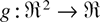
defined as follows:

Lemma 2.2: For any

, define the function
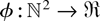
by

Then,

.
Proof: Without loss of generality, assume that s ≥ t ≥ 0. Then,

which holds if

However, this is true since gy(y) = 0 and gy(x) is increasing in

. Therefore,

. █
We are now in a position to prove Theorems 1.1–1.3.
Proof of Theorem 1.1: Let

denote the probability mass functions of X1 and Y1, respectively, and assume without loss of generality that {X1,…,Xn} and {Y1,…,Yn} are independent. From Eq. (1.1), it follows that for each

,

Note that X ≥lr Y implies pjX/pjY is increasing in j. Hence, to prove XI ≥lr YI, it suffices to prove that for each r = 2,…,n,
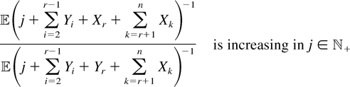
or, equivalently,

where

.
Let W be a random variable which has the same distribution as W and is independent of everything else. Then, Eq. (2.3) reduces to

We now turn to prove Eq. (2.4). To do so, set ψ(x,y;s,t) = φs,t(x,y) for each fixed

, where ψs,t is defined by Eq. (2.1). Then,
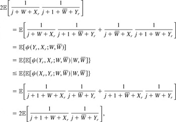
where the inequality follows from Lemmas 2.1 and 2.2 and the assumption that Xr ≥lr Yr. This establishes Eq. (2.4) and, thus, completes the proof. █
Proof of Theorem 1.2: Let

for k ≥ 1. It follows from Eq. (1.1) that to prove XIn ≤lr XIn+1, it suffices to prove that

is increasing in

, so we need to prove that

Let Tn−1 and Sn−1 be i.i.d. such that Tn−1 is independent of Xn, and let ψ(x,y;s,t) be as defined in the proof of Theorem 1.1. Then,

where the inequality follows from Lemmas 2.1 and 2.2 and the fact that 0 ≤lr Xn. This completes the proof. █
Proof of Theorem 1.3: First, note that

Since X1 ∈ PF2 implies that pj /pj+1 is increasing in j, to prove XI ∈ PF2 we need to verify that

or, equivalently,
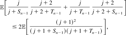
where Sn−1 and Tn−1 are i.i.d.
In order to prove Eq. (2.6), it suffices to verify that for

,
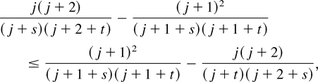
which is equivalent to

(abbreviated to L1 /L11 ≤ L2 /L22). By cumbersome simplification, it can be checked that

implying Eq. (2.7). This completes the proof. █
Remarks:
1. In Theorem 1.1, the likelihood ratio order cannot be replaced by the usual stochastic order; that is, X ≥st Y does not in general imply XI ≥st YI, as shown by the following counterexample. For n = 2, let the mass function of X1 be

and let the mass function of Y1 be

. It is easy to see that X ≥st Y but X [nge ]hr Y. From Eq. (1.1), it follows that

which implies that XI [nge ]st YI. It is still an open problem whether X ≥hr Y implies XI ≥hr YI or XI ≥st YI.
2. It is well known that X is PF2 if and only if X ≤lr X + x for all

(see Theorem 1.C.22 of [4]). Observing this, one might believe that Theorem 1.3 is a direct consequence of Theorem 1.1 by using

However, the assertion (2.8) is, in general, not correct, as shown by the following counterexample. Let n = 2, p1 = p2 = ½, and x = 1. It is easy to check that

implying that Eq. (2.8) is not true. It is still an open problem whether X being IFR (increasing failure rate) implies that XI is IFR. For the definition of IFR, see Barlow and Proschan [1].
3. Theorem 1.3 states that the PF2 property or logconcavity is preserved under the inspection paradox. However, the logconvexity is not, in general, preserved, as shown by the following counterexample. Let n = 2 and X be a geometric random variable with mass function

, where q = 1 − p ∈ (0,1). It is seen that pj is logconvex in

and that
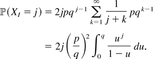
Then,

which imply that

is not increasing in

when p is small enough. Therefore,

is not logconvex in

for some p.
4. Let {N(t),t ≥ 0} be a renewal process with interarrival times

, where the Xi are i.i.d. The random variable XN(t)+1 represents the length of the renewal interval that contains the time point t. The inspection paradox of renewal theory is well known in the literature, which states that XN(t)+1 ≥st X1. In fact, it was shown in [3] that XN(t)+1 ≥lr X1 if X is absolutely continuous. Future research would be necessary to investigate some stochastic comparisons and preservation properties for this model. Such a study is more difficult and might be done elsewhere.
Acknowledgments
This work was supported by the National Natural Science Foundation of China (grant No. 10171093) and one grant from the Chinese Academy of Sciences.
References
REFERENCES
Barlow, R.E. &
Proschan, F.
(1975).
Statistical theory of reliability and life testing.
New York:
Holt, Rinehart, and Winston.
Müller, A. &
Stoyan, D.
(2002).
Comparison methods for stochastic models and risks.
West Sussex:
Wiley.
Ross, S.M.
(2003).
The inspection paradox.
Probability in Engineering and Informational Sciences
17:
47–51.Google Scholar
Shaked, M. &
Shanthikumar, J.G.
(1994).
Stochastic orders and their applications.
New York:
Academic Press.
Shanthikumar, J.G. &
Yao, D.
(1991).
Bivariate characterization of some stochastic order relations.
Advances in Applied Probability
23:
642–659.Google Scholar
 You have
Access
- 1
- Cited by