1 Introduction
Rao, Shukla & Yu (Reference Rao, Shukla and Yu1990) have first theoretically predicted the existence of extremely low phase speed dust-acoustic (DA) waves in which inertia (restoring force) is provided by the dust mass (thermal pressure of electrons and ions). This theoretical prediction of Rao et al. (Reference Rao, Shukla and Yu1990) has then been conclusively verified by Barkan, Merlino & D’Angelo (Reference Barkan, Merlino and D’Angelo1995). The discovery of the DA waves (Rao et al. Reference Rao, Shukla and Yu1990; Barkan et al. Reference Barkan, Merlino and D’Angelo1995) leads to a number investigations (Eliasson & Shukla Reference Eliasson and Shukla2004; Heinrich, Kim & Merlino Reference Heinrich, Kim and Merlino2009; Mamun & Cairns Reference Mamun and Cairns2009; Shukla & Eliasson Reference Shukla and Eliasson2012; Dev, Sharma & Deka Reference Dev, Sharma and Deka2015a ) on DA shock waves not only from theoretical points of view (Eliasson & Shukla Reference Eliasson and Shukla2004; Mamun & Cairns Reference Mamun and Cairns2009; Shukla & Eliasson Reference Shukla and Eliasson2012; Dev et al. Reference Dev, Sharma and Deka2015a ), but also from the view of laboratory experiments (Heinrich et al. Reference Heinrich, Kim and Merlino2009). The theoretical works (Eliasson & Shukla Reference Eliasson and Shukla2004; Mamun & Cairns Reference Mamun and Cairns2009; Shukla & Eliasson Reference Shukla and Eliasson2012; Dev et al. Reference Dev, Sharma and Deka2015a ) are based on a three-component dusty plasma system containing charged dust species of single polarity, and electron and ion species following the Maxwellian distribution function.
The electron and ion species do not only follow a Maxwellian distribution, but also follow various non-thermal distribution functions depending on space and laboratory plasma situations. The most commonly used non-thermal distribution function is the Schamel distribution function (Schamel Reference Schamel1972, Reference Schamel1973, Reference Schamel1986) which explains the trapping of the electron or/and ion species in many space and laboratory plasma situations (Schamel Reference Schamel1986; Andersson et al. Reference Andersson, Ergun, Newman, McFadden, Carlson and Su2002; Ergun et al. Reference Ergun, Andersson, Main and Su2002), where a significant part of the electron or/and ion species is confined to a finite region of phase space, and is forced to bounce back and forth (Schamel Reference Schamel1972, Reference Schamel1973, Reference Schamel1986). The effects of trapped electrons on ion-acoustic solitary waves was first examined by Schamel (Reference Schamel1973). It has also been observed by numerical simulation that a significant amount of the ion species is trapped in the wave potential of the DA waves (Winske et al. Reference Winske, Gary, Jones, Rosenberg, Chow and Mendis1995). The effects of trapped ion species on DA shock waves have been studied by a number of authors (Adhikary et al. Reference Adhikary, Deka, Dev and Sarma2014; Dev et al. Reference Dev, Sharma, Deka and Adhikary2015b ; El-Hanbaly et al. Reference El-Hanbaly, El-Shewy, Sallah and Darweesh2015; Adhikary et al. Reference Adhikary, Misra, Deka and Dev2017) who have shown the existence of the DA shock waves with stronger nonlinearity in a dusty plasma system containing a negatively charged dust fluid (Rao et al. Reference Rao, Shukla and Yu1990), ion species following the Schamel distribution function (Schamel Reference Schamel1972), and an electron species following the Maxwellian distribution function.
Recently, the study of linear (D’Angelo Reference D’Angelo2001, Reference D’Angelo2002; Shukla & Rosenberg Reference Shukla and Rosenberg2006) and nonlinear (Mamun & Shukla Reference Mamun and Shukla2002; Sayed & Mamun Reference Sayed and Mamun2007; Mamun Reference Mamun2008; Verheest Reference Verheest2009; Mamun & Schlickeiser Reference Mamun and Schlickeiser2015, Reference Mamun and Schlickeiser2016) DA waves in plasmas with micron or sub-micron sized charged dust grains of opposite polarity has received a great deal of attention because of their direct relevance to different regions of space (Chow, Mendis & Rosenberg Reference Chow, Mendis and Rosenberg1993; Horányi, Morfill & Grun Reference Horányi, Morfill and Grun1993; Mendis & Rosenberg Reference Mendis and Rosenberg1994; Havnes et al. Reference Havnes, Troim, Blix, Mortensen, Naesheim, Thrane and Tonnesen1996) and different laboratory devices (Trigwell et al. Reference Trigwell, Grable, Yurteri, Sharma and Mazumder2003; Zhao et al. Reference Zhao, Castle, Inculet and Bailey2003). Mamun & Shukla (Reference Mamun and Shukla2002) have considered a two-component dusty plasma system containing a dust fluid of opposite polarity, and studied the arbitrary amplitude DA solitary waves. Sayed & Mamun (Reference Sayed and Mamun2007) considered a four-component dusty plasma containing dust fluids of opposite polarity, and Boltzmann distributed electrons and ions, and showed the existence small amplitude DA solitary waves with either a positive or negative potential depending on the dusty plasma parameters by deriving the standard Korteweg–de Vries (KdV) equation. Mamun (Reference Mamun2008) has considered the same model of Sayed & Mamun (Reference Sayed and Mamun2007), and showed the coexistence of arbitrary amplitude DA solitary waves with both positive and negative potentials. Verheest (Reference Verheest2009) have considered plasmas with negative and positive cold dust fluids, and non-thermal electrons and ions, and have shown the coexistence of arbitrary amplitude DA solitary waves along with double layers. Mamun & Schlickeiser (Reference Mamun and Schlickeiser2015, Reference Mamun and Schlickeiser2016) have considered a self-gravitating opposite polarity dust–plasma medium, and examined the effects of the self-gravitational field on the formation of the solitary (Mamun & Schlickeiser Reference Mamun and Schlickeiser2015) and shock (Mamun & Schlickeiser Reference Mamun and Schlickeiser2016) waves by deriving the standard KdV (Burgers) equation. To the best knowledge of the authors, up to now, no investigation has been made of the effect of trapped electrons or ions on the shock waves formed in an opposite polarity dust–plasma medium. Therefore, in our present work, we consider an opposite polarity dust–plasma system containing a cold, viscous dust fluid of opposite polarity, ions following the Schamel distribution function (Schamel Reference Schamel1972, Reference Schamel1973, Reference Schamel1986) and electrons following the Maxwellian distribution function, and study the effects of the ion trapped distribution on the DA shock waves, which are found to exist in such an opposite polarity dust–plasma system.
This manuscript is structured as follows. The governing equations are provided in § 2. The modified Burgers (MB) equation and its analytical solution is derived in § 3. The basic features of the DA shock waves are identified by the numerical analysis of the analytical solution of the MB equation in the same section (§ 3). A brief discussion is finally presented in § 4.
2 Governing equations
We consider the nonlinear propagation of the DA waves in an unmagnetized dusty plasma system containing cold, viscous charged dust fluids of opposite polarity, ions following a Schamel distribution function (Schamel Reference Schamel1972, Reference Schamel1973, Reference Schamel1986) and Boltzmann distributed electrons (Rao et al. Reference Rao, Shukla and Yu1990). It is assumed that the phase speed of the DA waves is much lower than the thermal speeds of electrons and ions, but much higher than that of the positively and negatively charged dust. The nonlinear dynamics of these low frequency DA waves in such a dusty plasma system is described by the normalized equations in the form
 $$\begin{eqnarray}\displaystyle & \displaystyle \frac{\unicode[STIX]{x2202}n_{1}}{\unicode[STIX]{x2202}t}+\frac{\unicode[STIX]{x2202}}{\unicode[STIX]{x2202}x}(n_{1}u_{1})=0, & \displaystyle\end{eqnarray}$$
 $$\begin{eqnarray}\displaystyle & \displaystyle \frac{\unicode[STIX]{x2202}u_{1}}{\unicode[STIX]{x2202}t}+u_{1}\frac{\unicode[STIX]{x2202}u_{1}}{\unicode[STIX]{x2202}x}=\frac{\unicode[STIX]{x2202}\unicode[STIX]{x1D713}}{\unicode[STIX]{x2202}x}+\unicode[STIX]{x1D702}_{1}\frac{\unicode[STIX]{x2202}^{2}u_{1}}{\unicode[STIX]{x2202}x^{2}}, & \displaystyle\end{eqnarray}$$
 $$\begin{eqnarray}\displaystyle & \displaystyle \frac{\unicode[STIX]{x2202}n_{2}}{\unicode[STIX]{x2202}t}+\frac{\unicode[STIX]{x2202}}{\unicode[STIX]{x2202}x}(n_{2}u_{2})=0, & \displaystyle\end{eqnarray}$$
 $$\begin{eqnarray}\displaystyle & \displaystyle \frac{\unicode[STIX]{x2202}u_{2}}{\unicode[STIX]{x2202}t}+u_{2}\frac{\unicode[STIX]{x2202}u_{2}}{\unicode[STIX]{x2202}x}=-\unicode[STIX]{x1D6FC}\frac{\unicode[STIX]{x2202}\unicode[STIX]{x1D713}}{\unicode[STIX]{x2202}x}+\unicode[STIX]{x1D702}_{2}\frac{\unicode[STIX]{x2202}^{2}u_{2}}{\unicode[STIX]{x2202}x^{2}}, & \displaystyle\end{eqnarray}$$
 $$\begin{eqnarray}\displaystyle & \displaystyle \frac{\unicode[STIX]{x2202}^{2}\unicode[STIX]{x1D713}}{\unicode[STIX]{x2202}x^{2}}=n_{1}-\unicode[STIX]{x1D707}n_{2}+\unicode[STIX]{x1D707}_{e}e^{\unicode[STIX]{x1D70E}\unicode[STIX]{x1D713}}-\unicode[STIX]{x1D707}_{i}n_{i}, & \displaystyle\end{eqnarray}$$
where
 $n_{1}$
(
 $n_{2}$
)
 $n_{i}$
is the negative dust (positive dust) ion number density normalized by its equilibrium value
 $n_{10}$
(
 $n_{20}$
)
 $n_{i0}$
;
 $Z_{1}(Z_{2})$
is the number of electrons (protons) residing on a negative (positive) dust grain’s surface;
 $m_{1}$
(
 $m_{2}$
) is the mass of the negative (positive) dust grain;
 $u_{1}$
(
 $u_{2}$
) is the negative (positive) dust fluid speed normalized by
 $C_{1}=(Z_{1}k_{B}T_{i}/m_{1})^{1/2}$
in which
 $k_{B}$
(
 $T_{i}$
) is the Boltzmann constant (ion temperature);
 $\unicode[STIX]{x1D713}$
is the electrostatic wave potential normalized by
 $k_{B}T_{i}/e$
(with
 $e$
being the magnitude of the charge of an electron);
 $\unicode[STIX]{x1D702}_{1}$
(
 $\unicode[STIX]{x1D702}_{2}$
) is the viscosity coefficient normalized by
 $m_{1}n_{10}\unicode[STIX]{x1D714}_{p1}\unicode[STIX]{x1D706}_{D}^{2}$
(
 $m_{2}n_{20}\unicode[STIX]{x1D714}_{p1}\unicode[STIX]{x1D706}_{D}^{2}$
) for a negative (positive) dust fluid component;
 $t$
is the time variable normalized by the inverse of the negative dust plasma frequency
 $\unicode[STIX]{x1D714}_{p1}^{-1}=[4\unicode[STIX]{x03C0}Z_{1}^{2}e^{2}n_{10}/m_{1}]^{-1/2}$
;
 $x$
is the space variable normalized by the Debye radius
 $\unicode[STIX]{x1D706}_{D}=(Z_{1}k_{B}T_{i}/4\unicode[STIX]{x03C0}Z_{1}^{2}e^{2}n_{10})^{1/2}$
;
 $\unicode[STIX]{x1D6FC}=Z_{2}m_{1}/Z_{1}m_{2}$
,
 $\unicode[STIX]{x1D707}_{e}=n_{e0}/Z_{1}n_{10}$
,
 $\unicode[STIX]{x1D707}_{i}=n_{i0}/Z_{1}n_{10}$
and
 $\unicode[STIX]{x1D70E}=T_{i}/T_{e}$
in which
 $T_{e}$
is the electron temperature. We note that the coefficient
 $\unicode[STIX]{x1D707}=Z_{2}n_{20}/Z_{1}n_{10}=1+\unicode[STIX]{x1D707}_{e}-\unicode[STIX]{x1D707}_{i}$
of
 $n_{2}$
in (2.5) is determined from the charge neutrality condition at equilibrium (viz.,
 $n_{i0}+Z_{2}n_{20}=n_{e0}+Z_{1}n_{10}$
).
To study small, but finite amplitude nonlinear structures,
 $n_{i}$
can be expressed as (Schamel Reference Schamel1973)
 $$\begin{eqnarray}\displaystyle & \displaystyle n_{i}=1-\unicode[STIX]{x1D713}-\frac{4(1-\unicode[STIX]{x1D6FD})}{3\sqrt{\unicode[STIX]{x03C0}}}(-\unicode[STIX]{x1D713})^{3/2}+\frac{1}{2}\unicode[STIX]{x1D713}^{2}, & \displaystyle\end{eqnarray}$$
where
 $\unicode[STIX]{x1D6FD}$
, defined as the ratio of the free ion temperature (
 $T_{i}$
) to the trapped ion temperature (
 $T_{it}$
), is a parameter determining the number of trapped ions (Schamel Reference Schamel1972, Reference Schamel1973, Reference Schamel1986). We note that
 $\unicode[STIX]{x1D6FD}<0$
represents a vortex-like excavated trapped ion distribution and
 $\unicode[STIX]{x1D6FD}=1$
(
 $\unicode[STIX]{x1D6FD}=0$
) represents a Maxwellian (flat-topped) distribution.
3 MB equation
To derive the MB or modified Korteweg–de Vries (MKdV) equation from the governing equation one must find an appropriate coordinate frame in which the motion of the wave can be described smoothly. Actually, stretching the coordinates helps to see in detail what happens at different scales in distance or time.
To include the effects of trapped electrons (Schamel Reference Schamel1973) on ion-acoustic solitary waves, Schamel (Reference Schamel1973) first derived the MKdV equation by introducing stretching coordinates:
 $\unicode[STIX]{x1D709}=\unicode[STIX]{x1D716}^{1/4}(x-V_{p}t)$
and
 $\unicode[STIX]{x1D70F}=\unicode[STIX]{x1D716}^{3/4}t$
, where
 $\unicode[STIX]{x1D716}$
is a smallness parameter measuring the weakness of the dispersion (
 $0<\unicode[STIX]{x1D716}<1$
) and
 $V_{p}$
is the phase speed of the waves under consideration. The use of these stretching coordinates is valid when the effect of dissipation is negligible in comparison with that of dispersion. On the other hand, for the opposite situation, where the effect of dispersion is negligible in comparison with that of dissipation, Mamun & Shukla (Reference Mamun and Shukla2010) have modified these stretching coordinates in the form
 $\unicode[STIX]{x1D709}=\unicode[STIX]{x1D716}^{1/2}(x-V_{p}t)$
and
 $\unicode[STIX]{x1D70F}=\unicode[STIX]{x1D716}t$
, and have derived the MB equation, where the effects of trapped electrons and dissipation are included. These stretching coordinates have then been used by many authors (e.g. Adhikary et al. (Reference Adhikary, Deka, Dev and Sarma2014), Dev et al. (Reference Dev, Sharma and Deka2015a
), Adhikary et al. (Reference Adhikary, Misra, Deka and Dev2017), etc.) in order to derive the MB equation. Therefore, to include the combined effects of nonlinearity (due to trapped ions) and viscous forces acting in dust fluids of opposite polarity, we use the stretching coordinates (Mamun & Shukla Reference Mamun and Shukla2010; Adhikary et al.
Reference Adhikary, Deka, Dev and Sarma2014; Dev et al.
Reference Dev, Sharma and Deka2015a
; Adhikary et al.
Reference Adhikary, Misra, Deka and Dev2017),
 $$\begin{eqnarray}\left.\begin{array}{@{}c@{}}\unicode[STIX]{x1D709}=\unicode[STIX]{x1D716}^{1/2}(x-V_{p}t),\\ \unicode[STIX]{x1D70F}=\unicode[STIX]{x1D716}t,\end{array}\right\}\end{eqnarray}$$
and expand the variables
 $n_{s}$
,
 $u_{s}$
and
 $\unicode[STIX]{x1D713}$
, in power series of
 $\unicode[STIX]{x1D716}$
(Schamel Reference Schamel1973; Mamun & Shukla Reference Mamun and Shukla2010; Adhikary et al.
Reference Adhikary, Deka, Dev and Sarma2014):
 $$\begin{eqnarray}\displaystyle n_{s}=1+\unicode[STIX]{x1D716}n_{s}^{(1)}+\unicode[STIX]{x1D716}^{3/2}n_{s}^{(2)}+\cdots \,, & & \displaystyle\end{eqnarray}$$
 $$\begin{eqnarray}\displaystyle u_{s}=0+\unicode[STIX]{x1D716}u_{s}^{(1)}+\unicode[STIX]{x1D716}^{3/2}u_{s}^{(2)}+\cdots \,, & & \displaystyle\end{eqnarray}$$
 $$\begin{eqnarray}\displaystyle \unicode[STIX]{x1D713}=0+\unicode[STIX]{x1D716}\unicode[STIX]{x1D713}^{(1)}+\unicode[STIX]{x1D716}^{3/2}\unicode[STIX]{x1D713}^{(2)}+\cdots \,, & & \displaystyle\end{eqnarray}$$
where
 $s=1(2)$
stands for negative (positive) dust species. We use (2.6)–(3.4) in (2.1)–(2.5), and develop equations in various powers of
 $\unicode[STIX]{x1D716}$
. To the lowest order in
 $\unicode[STIX]{x1D716}$
, we have
 $$\begin{eqnarray}\displaystyle & \displaystyle n_{1}^{(1)}=-\frac{1}{V_{p}^{2}}\unicode[STIX]{x1D713}^{(1)}, & \displaystyle\end{eqnarray}$$
 $$\begin{eqnarray}\displaystyle & \displaystyle u_{1}^{(1)}=-\frac{1}{V_{p}}\unicode[STIX]{x1D713}^{(1)}, & \displaystyle\end{eqnarray}$$
 $$\begin{eqnarray}\displaystyle & \displaystyle n_{2}^{(1)}=\frac{\unicode[STIX]{x1D6FC}}{V_{p}^{2}}\unicode[STIX]{x1D713}^{(1)}, & \displaystyle\end{eqnarray}$$
 $$\begin{eqnarray}\displaystyle & \displaystyle u_{2}^{(1)}=\frac{\unicode[STIX]{x1D6FC}}{V_{p}}\unicode[STIX]{x1D713}^{(1)}, & \displaystyle\end{eqnarray}$$
 $$\begin{eqnarray}\displaystyle & \displaystyle V_{p}=\sqrt{\frac{1+\unicode[STIX]{x1D707}\unicode[STIX]{x1D6FC}}{\unicode[STIX]{x1D707}_{i}+\unicode[STIX]{x1D707}_{e}\unicode[STIX]{x1D70E}}}. & \displaystyle\end{eqnarray}$$
This expression for
 $V_{p}=\unicode[STIX]{x1D714}/k$
(where
 $\unicode[STIX]{x1D714}$
(
 $k$
) is the angular frequency (propagation constant)) represented by (3.9) provides the linear dispersion relation for the DA waves propagating in the opposite polarity dust–plasma medium under consideration. This dispersion relation indicates that the DA waves under condition are stable since
 $\unicode[STIX]{x1D707}=Z_{2}n_{2}/Z_{1}n_{1}\geqslant 0$
, where
 $\unicode[STIX]{x1D707}=0$
means no positive dust fluid component. The dispersion relation implies that, for fixed normalizing quantities (derived from dust mass and charge density of negative dust and ion temperature), the phase speed
 $V_{p}$
increases with the increase in charge density and the mass of positive dust, and the electron temperature, but decreases with the increase in the electron and ion number densities. We note that only the part of the free (but not part of the trapped) ions following the Schamel distribution function (Schamel Reference Schamel1973) participate in the linear propagation of the DA waves.
To the next higher order in
 $\unicode[STIX]{x1D716}$
, we obtain a set of equations in the form
 $$\begin{eqnarray}\displaystyle & \displaystyle \frac{\unicode[STIX]{x2202}n_{1}^{(1)}}{\unicode[STIX]{x2202}\unicode[STIX]{x1D70F}}-V_{p}\frac{\unicode[STIX]{x2202}n_{1}^{(2)}}{\unicode[STIX]{x2202}\unicode[STIX]{x1D709}}+\frac{\unicode[STIX]{x2202}u_{1}^{(2)}}{\unicode[STIX]{x2202}\unicode[STIX]{x1D709}}=0, & \displaystyle\end{eqnarray}$$
 $$\begin{eqnarray}\displaystyle & \displaystyle \frac{\unicode[STIX]{x2202}u_{1}^{(1)}}{\unicode[STIX]{x2202}\unicode[STIX]{x1D70F}}-V_{p}\frac{\unicode[STIX]{x2202}u_{1}^{(2)}}{\unicode[STIX]{x2202}\unicode[STIX]{x1D709}}-\frac{\unicode[STIX]{x2202}\unicode[STIX]{x1D713}^{(2)}}{\unicode[STIX]{x2202}\unicode[STIX]{x1D709}}-\unicode[STIX]{x1D702}_{1}\frac{\unicode[STIX]{x2202}^{2}u_{1}^{(1)}}{\unicode[STIX]{x2202}\unicode[STIX]{x1D709}^{2}}=0, & \displaystyle\end{eqnarray}$$
 $$\begin{eqnarray}\displaystyle & \displaystyle \frac{\unicode[STIX]{x2202}n_{2}^{(1)}}{\unicode[STIX]{x2202}\unicode[STIX]{x1D70F}}-V_{p}\frac{\unicode[STIX]{x2202}n_{2}^{(2)}}{\unicode[STIX]{x2202}\unicode[STIX]{x1D709}}+\frac{\unicode[STIX]{x2202}u_{2}^{(2)}}{\unicode[STIX]{x2202}\unicode[STIX]{x1D709}}=0, & \displaystyle\end{eqnarray}$$
 $$\begin{eqnarray}\displaystyle & \displaystyle \frac{\unicode[STIX]{x2202}u_{2}^{(1)}}{\unicode[STIX]{x2202}\unicode[STIX]{x1D70F}}-V_{p}\frac{\unicode[STIX]{x2202}u_{2}^{(2)}}{\unicode[STIX]{x2202}\unicode[STIX]{x1D709}}+\unicode[STIX]{x1D6FC}\frac{\unicode[STIX]{x2202}\unicode[STIX]{x1D713}^{(2)}}{\unicode[STIX]{x2202}\unicode[STIX]{x1D709}}-\unicode[STIX]{x1D702}_{2}\frac{\unicode[STIX]{x2202}^{2}u_{2}^{(1)}}{\unicode[STIX]{x2202}\unicode[STIX]{x1D709}^{2}}=0, & \displaystyle\end{eqnarray}$$
 $$\begin{eqnarray}\displaystyle & \displaystyle n_{1}^{(2)}-\unicode[STIX]{x1D707}n_{2}^{(2)}+\unicode[STIX]{x1D707}_{e}\unicode[STIX]{x1D70E}\unicode[STIX]{x1D713}^{(2)}+\unicode[STIX]{x1D707}_{i}\unicode[STIX]{x1D713}^{(2)}+\frac{4\unicode[STIX]{x1D707}_{i}(1-\unicode[STIX]{x1D6FD})}{3\sqrt{\unicode[STIX]{x03C0}}}(-\unicode[STIX]{x1D713}^{(1)})^{3/2}=0. & \displaystyle\end{eqnarray}$$
Now, using (3.5)–(3.14), one can eliminate
 $n_{1}^{(2)}$
,
 $n_{2}^{(2)}$
,
 $u_{1}^{(2)}$
,
 $u_{2}^{(2)}$
and
 $\unicode[STIX]{x1D713}^{(2)}$
, and can finally obtain
 $$\begin{eqnarray}\displaystyle & \displaystyle \frac{\unicode[STIX]{x2202}\unicode[STIX]{x1D713}^{(1)}}{\unicode[STIX]{x2202}\unicode[STIX]{x1D70F}}+A\sqrt{-\unicode[STIX]{x1D713}^{(1)}}\frac{\unicode[STIX]{x2202}\unicode[STIX]{x1D713}^{(1)}}{\unicode[STIX]{x2202}\unicode[STIX]{x1D709}}=C\frac{\unicode[STIX]{x2202}^{2}\unicode[STIX]{x1D713}^{(1)}}{\unicode[STIX]{x2202}\unicode[STIX]{x1D709}^{2}}, & \displaystyle\end{eqnarray}$$
where
 $A$
and
 $C$
are nonlinear and dissipative coefficients, and are given by
 $$\begin{eqnarray}\displaystyle & \displaystyle A=\frac{{V_{p}}^{3}\unicode[STIX]{x1D707}_{i}(1-\unicode[STIX]{x1D6FD})}{\sqrt{\unicode[STIX]{x03C0}}(1+\unicode[STIX]{x1D707}\unicode[STIX]{x1D6FC})}, & \displaystyle\end{eqnarray}$$
 $$\begin{eqnarray}\displaystyle & \displaystyle C=\frac{1}{2(\unicode[STIX]{x1D6FE}_{m}+\unicode[STIX]{x1D6FE}_{z})}[\unicode[STIX]{x1D6FE}_{m}\unicode[STIX]{x1D702}_{1}+\unicode[STIX]{x1D6FE}_{z}\unicode[STIX]{x1D702}_{2}+(1-\unicode[STIX]{x1D707})\unicode[STIX]{x1D6FE}_{m}(\unicode[STIX]{x1D702}_{1}-\unicode[STIX]{x1D702}_{2})], & \displaystyle\end{eqnarray}$$
in which
 $\unicode[STIX]{x1D6FE}_{m}=m_{2}/m_{1}$
and
 $\unicode[STIX]{x1D6FE}_{z}=Z_{2}/Z_{1}$
. Equation (3.15) is the MB equation describing the DA shock waves in plasmas with dusty fluids of opposite polarity, trapped ions and Boltzmann distributed electrons. This type of MB equation arises due to the balance between the nonlinearity, which is due to the trapped ions, and the dissipation, which is due to the viscous forces acting in dusty fluids of opposite polarity. We note that for
 $\unicode[STIX]{x1D702}_{1}\simeq \unicode[STIX]{x1D702}_{2}\simeq \unicode[STIX]{x1D702}$
, the dissipation coefficient represented by (3.17) reduces to
 $$\begin{eqnarray}C=\frac{\unicode[STIX]{x1D702}}{2}.\end{eqnarray}$$
Now, for a frame moving with a speed
 $U_{0}$
, the stationary localized solution (Adhikary et al.
Reference Adhikary, Deka, Dev and Sarma2014; Dev et al.
Reference Dev, Sharma, Deka and Adhikary2015b
; Adhikary et al.
Reference Adhikary, Misra, Deka and Dev2017) of the MB equation (3.19) is given by
 $$\begin{eqnarray}\displaystyle & \displaystyle \unicode[STIX]{x1D713}=-\unicode[STIX]{x1D713}_{m}^{2}\left[1-\tanh \left(\frac{\unicode[STIX]{x1D709}-U_{0}\unicode[STIX]{x1D70F}}{\unicode[STIX]{x1D6E5}}\right)\right]^{2}, & \displaystyle\end{eqnarray}$$
where
 $\unicode[STIX]{x1D713}$
,
 $\unicode[STIX]{x1D713}_{m}$
and
 $\unicode[STIX]{x1D6E5}$
are given by
 $$\begin{eqnarray}\displaystyle & \displaystyle \unicode[STIX]{x1D713}=\unicode[STIX]{x1D713}^{(1)} & \displaystyle\end{eqnarray}$$
 $$\begin{eqnarray}\displaystyle & \displaystyle \unicode[STIX]{x1D713}_{m}=\frac{3U_{0}}{4A}, & \displaystyle\end{eqnarray}$$
 $$\begin{eqnarray}\displaystyle & \displaystyle \unicode[STIX]{x1D6E5}=\frac{4C}{U_{0}}. & \displaystyle\end{eqnarray}$$
It is obvious that, as the speed
 $U_{0}$
increases, the amplitude (width) increases (decreases), and that the viscosity coefficient
 $\unicode[STIX]{x1D702}$
does not have any effect on the amplitude, but it does have significant effects on the width of the DA shock waves (as
 $\unicode[STIX]{x1D702}$
increases, the width of the DA shock waves increases significantly).
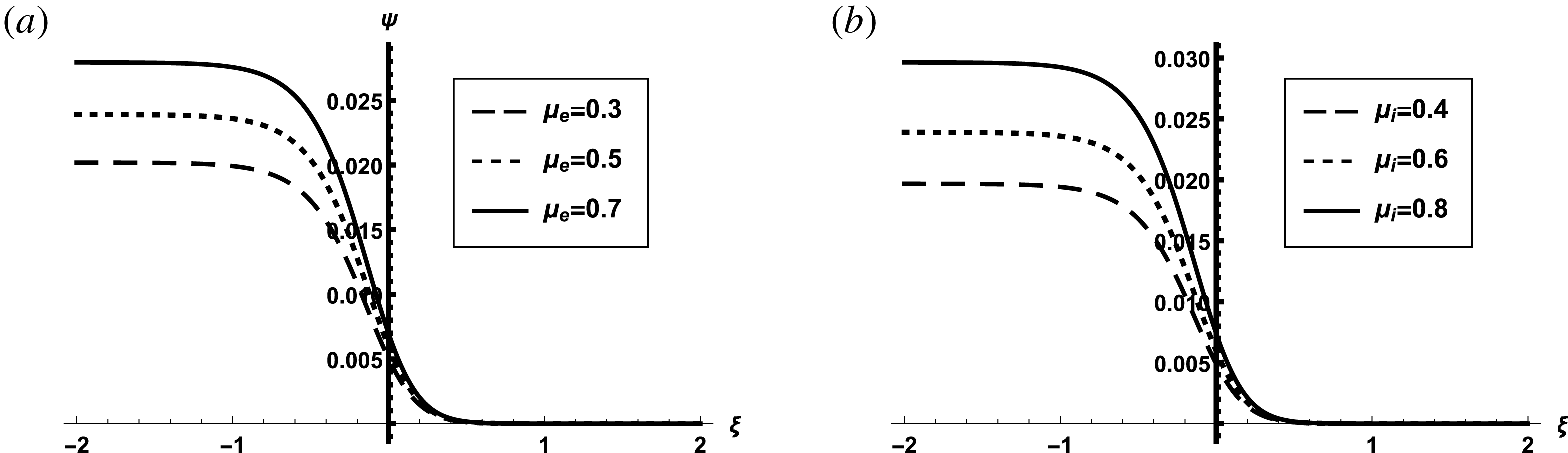
The shock profiles (
 $\unicode[STIX]{x1D713}$
versus
 $\unicode[STIX]{x1D709}$
curves) for three different values of
 $\unicode[STIX]{x1D707}_{e}$
along with
 $\unicode[STIX]{x1D707}_{i}=0.4$
(a) and for three different values of
 $\unicode[STIX]{x1D707}_{i}$
along with
 $\unicode[STIX]{x1D707}_{e}=0.3$
(b). The other parameters are always fixed (viz.
 $\unicode[STIX]{x1D6FC}=0.3$
,
 $\unicode[STIX]{x1D6FD}=-0.5$
,
 $\unicode[STIX]{x1D70E}=0.3$
and
 $\unicode[STIX]{x1D702}=0.02$
).

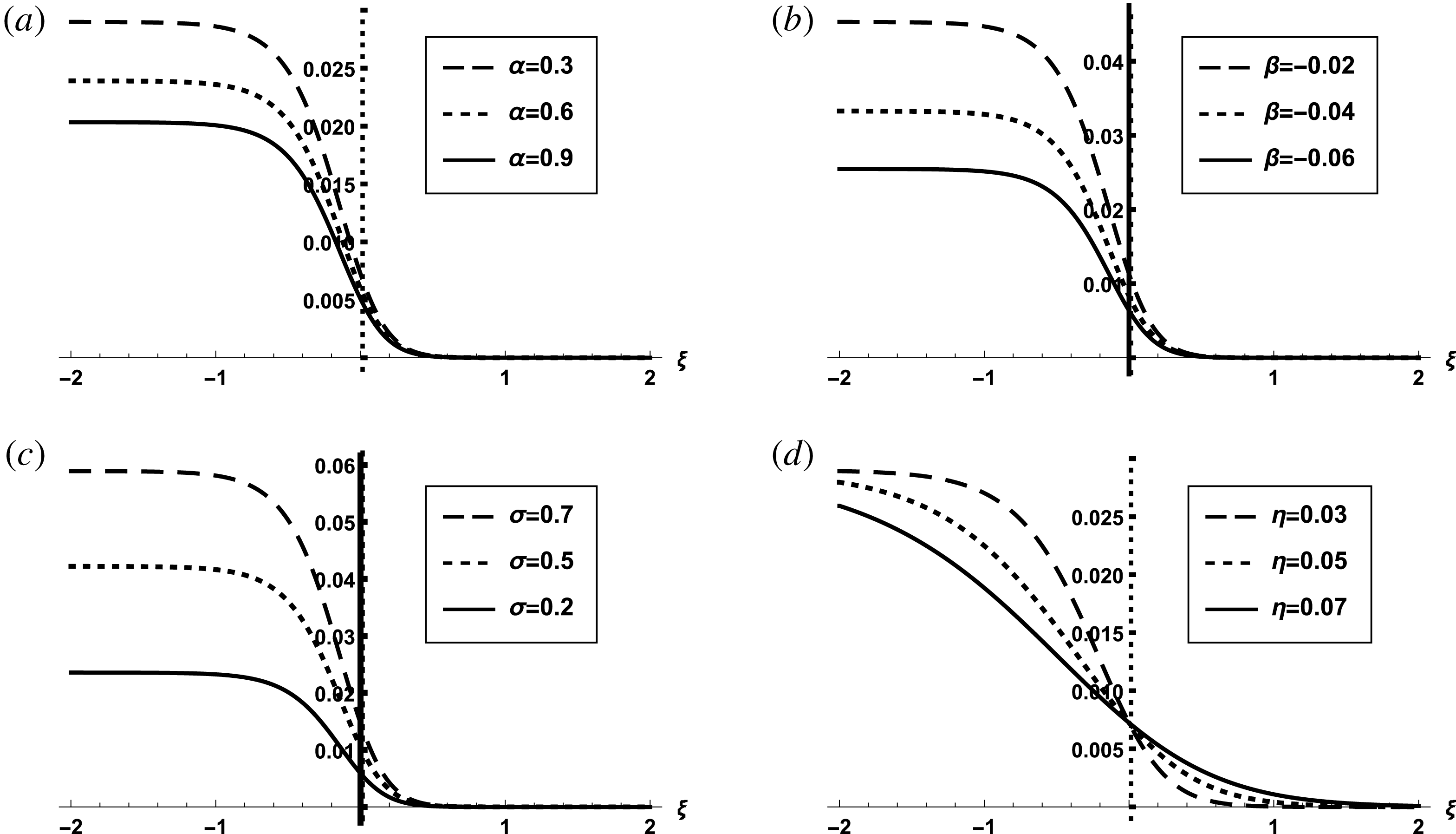
The shock profiles (
 $\unicode[STIX]{x1D713}$
versus
 $\unicode[STIX]{x1D709}$
curves) for three different values of
 $\unicode[STIX]{x1D6FC}$
along with fixed values of the other parameters,
 $\unicode[STIX]{x1D6FD}=-0.5$
,
 $\unicode[STIX]{x1D70E}=0.3$
and
 $\unicode[STIX]{x1D702}=0.02$
(a); for three different values of
 $\unicode[STIX]{x1D6FD}$
along with fixed values of the other parameters,
 $\unicode[STIX]{x1D6FC}=0.3$
,
 $\unicode[STIX]{x1D70E}=0.3$
and
 $\unicode[STIX]{x1D702}=0.02$
(b); for three different values of
 $\unicode[STIX]{x1D70E}$
along with fixed values of the other parameters,
 $\unicode[STIX]{x1D6FC}=0.3$
,
 $\unicode[STIX]{x1D6FD}=-0.5$
and
 $\unicode[STIX]{x1D702}=0.02$
(c); for three different values of
 $\unicode[STIX]{x1D702}$
along with fixed values of the other parameters,
 $\unicode[STIX]{x1D6FC}=0.3$
,
 $\unicode[STIX]{x1D6FD}=-0.5$
and
 $\unicode[STIX]{x1D70E}=0.3$
(d). The other two parameters,
 $\unicode[STIX]{x1D707}_{e}$
and
 $\unicode[STIX]{x1D707}_{i}$
are always fixed (viz.
 $\unicode[STIX]{x1D707}_{e}=0.6$
and
 $\unicode[STIX]{x1D707}_{i}=0.5$
).

To identify the effects of
 $\unicode[STIX]{x1D707}_{e}$
,
 $\unicode[STIX]{x1D707}_{i}$
 $\unicode[STIX]{x1D6FC}$
,
 $\unicode[STIX]{x1D6FD}$
,
 $\unicode[STIX]{x1D70E}$
and
 $\unicode[STIX]{x1D702}$
on the DA shock structures, we have numerically analysed the solution (3.19) of the MB equation (3.15). The numerical results are displayed in figures 1 and 2, which indicate that (i) the DA shock structures with stronger nonlinearity are formed with
 $\unicode[STIX]{x1D713}>0$
; (ii) the amplitude (width) of the DA shock structures increases (decreases) with the increase in the values of
 $\unicode[STIX]{x1D707}_{e}$
,
 $\unicode[STIX]{x1D707}_{i}$
,
 $\unicode[STIX]{x1D6FD}$
and
 $\unicode[STIX]{x1D70E}$
; (iii) the amplitude (width) of the DA shock structures decreases (increases) with the increase in the values
 $\unicode[STIX]{x1D6FC}$
and
 $\unicode[STIX]{x1D702}$
.
4 Discussion
We have considered the nonlinear propagation of the DA waves in an unmagnetized dusty plasma system containing cold, viscous charged dust fluids of opposite polarity, ions following the Schamel distribution function (Schamel Reference Schamel1972, Reference Schamel1973, Reference Schamel1986) and Maxwellian electrons. We have used the reductive perturbation method to derive the MB equation which gives rise to the DA shock waves with stronger nonlinearity. The results which have been obtained from this theoretical investigation can be pointed out as follows:
(i) The Schamel distribution function (Schamel Reference Schamel1972, Reference Schamel1973, Reference Schamel1986) has three regimes: two represent high energy free ions, and one in between these two regimes represents trapped ions. The free (trapped) ions participate in linear (nonlinear) propagation of the DA waves under consideration.
(ii) The DA waves under condition are stable since
 $\unicode[STIX]{x1D714}^{2}>0$
, and for fixed normalizing quantities (derived from the mass and charge density of negative dust and the ion temperature), the phase speed
$V_{p}$
increases with the increase in charge density and mass of the positive dust, and the electron temperature, but decreases with the increase in electron and ion number densities.
(iii) The viscosity of dust fluids of opposite polarity is the source of dissipation, and is responsible for the formation of the DA shock waves in plasmas with dust fluids of opposite polarity, trapped ions and Maxwellian electrons.
(iv) The DA shock structures with stronger nonlinearity are formed with
$\unicode[STIX]{x1D713}>0$
. Their amplitude (width) increases (decreases) with increase in the values of
$\unicode[STIX]{x1D707}_{e}$
,
$\unicode[STIX]{x1D707}_{i}$
,
$\unicode[STIX]{x1D6FD}$
and
$\unicode[STIX]{x1D70E}$
but their amplitude (width) decreases (increases) with the increase in the values of
$\unicode[STIX]{x1D6FC}$
and
$\unicode[STIX]{x1D702}$
.(v) The nonlinearity of the DA shock waves as the solution of the MB equation is much stronger than that as the solution of the standard Burgers equation. This stronger nonlinearity is due to the effect of the trapped ions.


The ranges of all the dusty plasma parameters (viz.,
 $\unicode[STIX]{x1D707}_{e}$
,
 $\unicode[STIX]{x1D707}_{i}$
,
 $\unicode[STIX]{x1D6FC}$
,
 $\unicode[STIX]{x1D6FD}$
,
 $\unicode[STIX]{x1D70E}$
and
 $\unicode[STIX]{x1D702}$
) used in this numerical analysis are very wide and are relevant to space (viz., cometary tails (Chow et al.
Reference Chow, Mendis and Rosenberg1993; Mendis & Rosenberg Reference Mendis and Rosenberg1994), the upper mesosphere (Havnes et al.
Reference Havnes, Troim, Blix, Mortensen, Naesheim, Thrane and Tonnesen1996), Jupiter’s magnetosphere (Horányi et al.
Reference Horányi, Morfill and Grun1993) and laboratory dusty plasma situations (Heinrich et al.
Reference Heinrich, Kim and Merlino2009). Therefore, the results of our present investigation should be useful to understanding of the nonlinear features of the electrostatic disturbances in space and laboratory dusty plasmas.
It is important to note that the stretching coordinates
 $\unicode[STIX]{x1D709}=\unicode[STIX]{x1D716}^{1/4}(x-V_{p}t)$
and
 $\unicode[STIX]{x1D70F}=\unicode[STIX]{x1D716}^{3/4}t$
, which are designed for the situation where the effect of dissipation for the wave under consideration is negligible in comparison with that of dispersion for the same, gives rise to the MKdV equation (Schamel Reference Schamel1973). On the other hand, the stretching coordinates
 $\unicode[STIX]{x1D709}=\unicode[STIX]{x1D716}^{1/2}(x-V_{p}t)$
and
 $\unicode[STIX]{x1D70F}=\unicode[STIX]{x1D716}t$
are designed for the opposite situation, where the effect of dispersion for the wave under consideration is negligible in comparison with that of dissipation for the same. Therefore, the nonlinear coefficients in the MKdV and MB equations are identical, but the dissipation (dispersion) terms disappears in the MKdV (MB) equation. It is observed that the nonlinearity in the MKdV and MB equations is stronger than that in standard KdV and Burgers equations.
To conclude, we propose to perform a new experiment to verify the results that we have presented in this work, and also expect to observe the effects of the important plasma parameters on DA shock structures in both laboratory and space plasmas with dust particles of opposite polarity and trapped particles.