2.1. Governing equations

We start from the inviscid, incompressible, hydrostatic and Boussinesq momentum, continuity and internal energy equations (e.g. Cushman-Roisin & Beckers Reference Cushman-Roisin and Beckers2011)

(2.1a)$$\begin{gather} \frac{\textrm{D} \boldsymbol{u}_{tot}(\boldsymbol{x},z,t)}{\textrm{D}t}+ \boldsymbol{f}\times\boldsymbol{u}_{tot}(\boldsymbol{x},z,t) ={-}\frac{1}{\rho_0}\boldsymbol{\nabla} p_{tot}(\boldsymbol{x},z,t), \end{gather}$$

(2.1b)$$\begin{gather}\frac{\partial p_{tot}(\boldsymbol{x},z,t)}{\partial z}+\rho_{tot}(\boldsymbol{x},z,t) g=0, \end{gather}$$

(2.1c)$$\begin{gather}\boldsymbol{\nabla} \boldsymbol{\cdot} \boldsymbol{u}_{tot}(\boldsymbol{x},z,t) + \frac{\partial w_{tot}(\boldsymbol{x},z,t)}{\partial z}=0, \end{gather}$$

(2.1d)$$\begin{gather}\frac{\textrm{D} \rho_{tot}(\boldsymbol{x},z,t)}{\textrm{D}t}=0, \end{gather}$$

where $\boldsymbol {x}\equiv (x,y)$ is the horizontal plane, $z$ is the upward vertical axis, $\boldsymbol {\nabla }\equiv (\partial /\partial x, \partial /\partial y)$ is the horizontal divergence operator, $t$ is the time, $\textrm {D}/\textrm {D}t$ the material derivative, and $\boldsymbol {u}_{tot}\equiv (u_{tot}, v_{tot}), w_{tot}, p_{tot}$ and $\rho _{tot}$ are respectively the total horizontal velocity, vertical velocity, pressure and density; $\boldsymbol {f}\equiv f\hat {z}$ with $f$ being the inertial (Coriolis) frequency and $\hat {z}$ the unit upward vector; $\rho _0$ is the reference density (due to the Boussinesq approximation) and $g$ the gravitational acceleration. We note that the hydrostatic approximation made in (2.1b) is generally valid for large-scale, lower-mode ITs, which are the focus of the present paper. Non-hydrostatic effects can be important for higher IT modes (e.g. in estuaries).

We consider the total field as a superposition of a rapidly evolving tidal flow field and a time-averaged (or slowly evolving) background field (e.g. Kunze Reference Kunze1985)

(2.2a)$$\begin{gather} \boldsymbol{u}_{tot}(\boldsymbol{x},z,t)=\boldsymbol{U}(\boldsymbol{x},z; t_0, \tau)+\boldsymbol{u}(\boldsymbol{x},z,t), \end{gather}$$

(2.2b)$$\begin{gather}w_{tot}(\boldsymbol{x},z,t)=W(\boldsymbol{x},z; t_0, \tau)+\boldsymbol{w}(\boldsymbol{x},z,t), \end{gather}$$

(2.2c)$$\begin{gather}\rho_{tot}(\boldsymbol{x},z,t)=\rho_0-\frac{\rho_0}{g}b_{tot}(\boldsymbol{x},z,t),\quad b_{tot}=B(\boldsymbol{x},z; t_0, \tau)+b(\boldsymbol{x},z,t), \end{gather}$$

(2.2d)$$\begin{gather}p_{tot}(\boldsymbol{x},z,t)=p_0(z)+P(\boldsymbol{x},z; t_0, \tau)+p(\boldsymbol{x},z,t), \end{gather}$$

where ($\boldsymbol {U}(\boldsymbol {x},z; t_0, \tau ), W(\boldsymbol {x},z; t_0, \tau )$) is the $[t_0, t_0+\tau ]$ time-averaged flow field defined by

(2.3a,b)\begin{equation} \boldsymbol{U} = \int_{t=t_0}^{t_0+\tau} \boldsymbol{u}_{tot} \, \textrm{d} t, \quad W = \int_{t=t_0}^{t_0+\tau} w_{tot} \, \textrm{d} t, \end{equation}

where $\tau$ is a time scale much larger than the tidal period; ($\boldsymbol {u}(\boldsymbol {x},z,t), w(\boldsymbol {x},z,t)$) is the oscillatory tidal flow field; and $b_{tot}(\boldsymbol {x},z,t) \equiv -g\rho '(\boldsymbol {x},z,t)/\rho _0$ is the buoyancy term that is further decomposed into its time-averaged $B(\boldsymbol {x},z; t_0, \tau )$ and oscillatory $b(\boldsymbol {x},z,t)$ parts, where $\rho '(\boldsymbol {x},z,t)\equiv \rho _{tot}(\boldsymbol {x},z,t)-\rho _0$ is the perturbed density due to stratification, mean flow and ITs. The hydrostatic pressures $p_0(z), P(\boldsymbol {x},z; t_0, \tau )$ and $p(\boldsymbol {x},z,t)$ are determined respectively from $\rho _0, B(\boldsymbol {x},z)$ and $b(\boldsymbol {x},z,t)$.

For notational simplicity, we will hereafter omit writing the dependence of the background field on $t_0$ and $\tau$, but one should keep in mind that the background field evolves slowly with a time scale $\tau$ that is (much) larger than the tidal period. The equations governing the small amplitude oscillatory tidal flow (Kelly & Lermusiaux Reference Kelly and Lermusiaux2016) are obtained by subtracting the time-averaged background part from the total (2.1) using (2.2) and neglecting the component of wave–wave interactions, which gives

(2.4a)$$\begin{gather} \frac{\partial \boldsymbol{u}}{\partial t}+(\boldsymbol{U}\boldsymbol{\cdot}\boldsymbol{\nabla})\boldsymbol{u} +(\boldsymbol{u}\boldsymbol{\cdot}\boldsymbol{\nabla})\boldsymbol{U} + w\frac{\partial \boldsymbol{U}}{\partial z} + W\frac{\partial \boldsymbol{u}}{\partial z} + \boldsymbol{f}\times\boldsymbol{u} ={-}\frac{1}{\rho_0}\boldsymbol{\nabla} p, \end{gather}$$

(2.4b)$$\begin{gather}\frac{1}{\rho_0}\frac{\partial p}{\partial z}-b=0, \end{gather}$$

(2.4c)$$\begin{gather}\boldsymbol{\nabla} \boldsymbol{\cdot} \boldsymbol{u} + \frac{\partial w}{\partial z}=0, \end{gather}$$

(2.4d)$$\begin{gather}\frac{\partial b}{\partial t}+(\boldsymbol{U}\boldsymbol{\cdot}\boldsymbol{\nabla})b +(\boldsymbol{u}\boldsymbol{\cdot}\boldsymbol{\nabla})B+W\frac{\partial b}{\partial z}+wN^2=0, \end{gather}$$

where $N(\boldsymbol {x},z)$ is the spatially varying background buoyancy frequency, with

(2.5)\begin{equation} N^2(\boldsymbol{x},z) \equiv \frac{\partial B}{\partial z}. \end{equation}

Note that, although we neglect the wave–wave interactions in (2.4), when we diagnose a full PE simulation the time average of the wave–wave interactions is fully preserved in the background fields (see (3) in Kelly & Lermusiaux Reference Kelly and Lermusiaux2016).

The tidal field is governed by (2.4) in a vertically bounded domain from $z=-H(\boldsymbol {x})$ to $z=0$. We assume simplified boundary conditions

(2.6)\begin{equation} w=0, \quad \text{at } z=0\ \text{and}\ z={-}H(\boldsymbol{x}). \end{equation}

The error introduced by (2.6) is of the same order as the small errors done in the hydrostatic approximation given that $\alpha \sim O(H/L)$, where $\alpha$ is the boundary slope due to surface elevation and sloping bottom topography, and $L$ is the horizontal scale. Specifically, for $\alpha \sim O(H/L)$, we neglect a vertical velocity component of $O(U_hH/L)$ in the flow field, where $U_h$ is the characteristic horizontal velocity. This approximation is of the same order as the hydrostatic approximation used to neglect the vertical velocity component in (2.4b) (Cushman-Roisin & Beckers Reference Cushman-Roisin and Beckers2011) and is therefore justified. This simplification facilitates the vertical-mode decomposition introduced in § 2.2, although more accurate ways to specify the boundary conditions exist (Griffiths & Grimshaw Reference Griffiths and Grimshaw2007; Kelly Reference Kelly2016). The ultimate validity of the derivation including this simplification can be evaluated by comparison with the PE simulations.

2.2. Projection onto vertical modes and CTE

We consider the tidal field described by (2.4) subject to (2.6). The traditional vertical decomposition of ITs can be obtained by considering constant topography, zero mean flow and zero horizontal buoyancy gradient. Under these conditions, (2.4) can be solved, leading to decoupled orthogonal vertical modes as the solution of an eigenvalue problem depending only on $N^2(z)$ and $H$. With the complexities added by the varying mean flow, topography and buoyancy frequency in (2.4), the decoupling of vertical modes is not possible (the horizontal variation of the background prohibits the vertical modes being independent of the horizontal location, and the depth-varying background renders the eigenvalue problem to be of the Taylor–Goldstein form, yielding non-orthogonal eigenmodes, see Duda et al. Reference Duda, Lin, Buijsman and Newhall2018; Huang et al. Reference Huang, Wang, Zhang, Yang, Zhou, Yang, Zhao and Tian2018). However, as in Kelly & Lermusiaux Reference Kelly and Lermusiaux2016, we can use a different treatment by decomposing the vertical tidal structure into prescribed orthogonal vertical modes determined from local $N^2(\boldsymbol {x},z)$ and $H(\boldsymbol {x})$, and deriving equations governing the evolution of the modal amplitudes at all locations in the horizontal plane. Although this treatment results in equations involving the coupling of the vertical modes, it is still desirable as it replaces the vertical dependence of ITs with modal representation. With the major dynamics of IT captured by the lowest few modes which contain most of the energy and propagate for a long distance (e.g. Nash et al. Reference Nash, Kunze, Lee and Sanford2006; Alford & Zhao Reference Alford and Zhao2007), the modal approach provides a reduced-order model for the IT.

Therefore, we consider the expansion of the IT field as a series of vertical modes (Kelly & Lermusiaux Reference Kelly and Lermusiaux2016)

(2.7a)$$\begin{gather} \boldsymbol{u}(\boldsymbol{x},z,t)=\sum_{n=0}^\infty \boldsymbol{u}_n(\boldsymbol{x},t)\phi_n(\boldsymbol{x},z,\tau), \end{gather}$$

(2.7b)$$\begin{gather}p(\boldsymbol{x},z,t)=\sum_{n=0}^\infty p_n(\boldsymbol{x},t)\phi_n(\boldsymbol{x},z,\tau), \end{gather}$$

(2.7c)$$\begin{gather}w(\boldsymbol{x},z,t)=\sum_{n=0}^\infty w_n(\boldsymbol{x},t)\varPhi_n(\boldsymbol{x},z,\tau), \end{gather}$$

(2.7d)$$\begin{gather}b(\boldsymbol{x},z,t)=\sum_{n=0}^\infty b_n(\boldsymbol{x},t)N^2(\boldsymbol{x},z)\varPhi_n(\boldsymbol{x},z,\tau), \end{gather}$$

where $n$ is the mode number, $\boldsymbol {u}_n(\boldsymbol {x},t), p_n(\boldsymbol {x},t), w_n(\boldsymbol {x},t)$ and $b_n(\boldsymbol {x},t)$ are modal amplitudes. Here, $\varPhi _n(\boldsymbol {x},z,\tau )$ and $\phi _n(\boldsymbol {x},z,\tau )$ are the vertical modes determined locally at each $\boldsymbol {x}$. As we did for the background fields, we will omit writing the dependency of the vertical modes on $\tau$. For $n \geq 1$, the internal baroclinic modes (mode-$1$ to mode-$n$) are defined by a prescribed eigenvalue problem (cf. Gill & Clarke Reference Gill and Clarke1974)

(2.8)\begin{equation} \frac{\partial^2 \varPhi_n}{\partial z^2} + \frac{N^2}{c_n^2}\varPhi_n=0,\quad \text{with}\ \varPhi_n(\boldsymbol{x},0)=\varPhi_n(\boldsymbol{x},-H)=0, \end{equation}

with $c_n$ being the eigenspeed, and

(2.9)\begin{equation} \phi_n(\boldsymbol{x},z)\equiv \frac{\partial \varPhi_n(\boldsymbol{x},z)}{\partial z}. \end{equation}

For $n=0$, we define the barotropic mode (mode-$0$) to be $\varPhi _0=0$ and $\phi _0$ as a non-zero constant (with values to be determined by specific normalization), satisfying the vertical dependence of the barotropic tidal flow. Under these definitions, the eigenfunctions $\varPhi _n(\boldsymbol {x},z)$ and $\phi _n(\boldsymbol {x},z)$ are both orthogonal at each location $\boldsymbol {x}$, and the boundary conditions in (2.6) are satisfied. We further choose a normalization

(2.10a)$$\begin{gather} \int_{{-}H}^0 N^2 \varPhi_m \varPhi_n \, \textrm{d} z = c_n^2 \delta_{mn},\quad n \geq 1, \end{gather}$$

(2.10b)$$\begin{gather}\int_{{-}H}^0 \phi_m \phi_n \, \textrm{d} z = \delta_{mn}, \end{gather}$$

where $\delta _{mn}$ is the Kronecker delta function. We note that the normalization used in (2.10) differs from that in Kelly & Lermusiaux (Reference Kelly and Lermusiaux2016) by a factor of $H$. This simplifies the form of the CTE when the co-varying features of the background fields are considered.

The momentum and pressure CTEs can then be derived by projecting (2.4) onto the vertical modes (2.7), (2.8) and (2.9). Due to the simultaneous consideration of mean flow in (2.4) and horizontally varying topography and buoyancy in (2.7), new three-way interaction terms can be expected, in contrast to the separate treatment in Kelly & Lermusiaux (Reference Kelly and Lermusiaux2016). Specifically, we depth integrate the product of (2.4a) with $\phi _n$, and the product of (2.4d) with $\varPhi _n$. From (2.4b) and (2.4c), $p_n$ is related to $b_n$, and $w_n$ to $u_n$ (where integration by parts and Leibniz's rule are used, see Kelly et al. Reference Kelly, Lermusiaux, Duda and Haley2016), and the projections of (2.4a) and (2.4d) lead to the CTEs

(2.11a)\begin{align} & \frac{\partial \boldsymbol{u}_n}{\partial t} + \sum_{m=0}^{\infty} \left[ (\boldsymbol{U}_{nm}\boldsymbol{\cdot}\boldsymbol{\nabla} + C_{nm} - W_{nm})\boldsymbol{u}_m + \boldsymbol{u}_m \boldsymbol{\cdot} \boldsymbol{\mathcal{U}}^g_{nm} + \left(\sum_{l=0}^{\infty}\boldsymbol{u}_l\boldsymbol{\cdot} \boldsymbol{T}_{ml}-\boldsymbol{\nabla}\boldsymbol{\cdot}\boldsymbol{u}_m\right)\boldsymbol{U}^z_{nm} \right] \nonumber\\ &\quad + \boldsymbol{f}\times\boldsymbol{u}_n ={-}\frac{1}{\rho_0} \left(\boldsymbol{\nabla} p_n + \sum_{m=0}^{\infty} p_m\boldsymbol{T}_{mn}\right), \end{align}

and

(2.11b)\begin{align} &\frac{\partial p_n}{\partial t} + \sum_{m=0}^{\infty} \left[ (\boldsymbol{U}^p_{nm} \boldsymbol{\cdot} \boldsymbol{\nabla} + C^p_{nm} + W^p_{nm})p_m - \rho_0\boldsymbol{u}_m\boldsymbol{\cdot} \boldsymbol{B}_{nm} \right]\nonumber\\ &\quad ={-}\rho_0 c_n^2 \boldsymbol{\nabla}\boldsymbol{\cdot} \boldsymbol{u}_n + \rho_0c_n^2\sum_{m=0}^{\infty} \boldsymbol{u}_m \boldsymbol{\cdot} \boldsymbol{T}_{nm}, \end{align}

where the momentum mode-coupling coefficients are defined as

(2.12a)$$\begin{gather} \boldsymbol{U}_{nm}=\int_{{-}H}^0 \boldsymbol{U} \phi_m \phi_n \, \textrm{d} z, \end{gather}$$

(2.12b)$$\begin{gather}\text{(*)}\quad C_{nm}=\int_{{-}H}^0 \boldsymbol{U} \boldsymbol{\cdot} \boldsymbol{\nabla} \phi_m \phi_n \, \textrm{d} z, \end{gather}$$

(2.12c)$$\begin{gather}W_{nm}=\int_{{-}H}^0 \frac{N^2}{c_m^2} W\varPhi_m \phi_n \, \textrm{d} z, \end{gather}$$

(2.12d)$$\begin{gather}{\boldsymbol{\mathcal{U}}}^g_{nm} = \int_{{-}H}^0 \boldsymbol{\nabla}\boldsymbol{U} \phi_m \phi_n \, \textrm{d} z, \end{gather}$$

(2.12e)$$\begin{gather}\boldsymbol{U}^z_{nm} = \int_{{-}H}^0 \frac{\partial \boldsymbol{U}}{\partial z} \varPhi_m \phi_n \, \textrm{d} z, \end{gather}$$

(2.12f)$$\begin{gather}\boldsymbol{T}_{nm}=\int_{{-}H}^0\phi_m\boldsymbol{\nabla}\phi_n \, \textrm{d} z, \end{gather}$$

(2.12g)$$\begin{gather}\boldsymbol{U}^p_{nm} = \int_{{-}H}^0 \boldsymbol{U} \frac{N^2}{c_m^2} \varPhi_m \varPhi_n \, \textrm{d} z, \end{gather}$$

(2.12h)$$\begin{gather}\text{(*)}\quad C^p_{nm} = \int_{{-}H}^0 \frac{\boldsymbol{U}}{c_m^2} \boldsymbol{\cdot} \boldsymbol{\nabla} (N^2\varPhi_m)\varPhi_n \, \textrm{d} z, \end{gather}$$

(2.12i)$$\begin{gather}W^p_{nm} = \int_{{-}H}^0 \frac{W}{c_m^2} \frac{\partial}{\partial z}(N^2\varPhi_m)\varPhi_n \, \textrm{d} z, \end{gather}$$

(2.12j)$$\begin{gather}\boldsymbol{B}_{nm} = \int_{{-}H}^0 \boldsymbol{\nabla} B \phi_m \varPhi_n \, \textrm{d} z, \end{gather}$$

and where we denoted the new three-way interaction terms with a ($*$). In (2.12), we use symbols $\boldsymbol {U}$ and $W$ (with subscript) to represent the coupling due to mean flow, $\boldsymbol {B}$ the coupling due to (only) horizontal buoyancy gradient, $\boldsymbol {T}$ the coupling due to horizontally varying topography and buoyancy and $C$ the coupling due to the co-existent mean flow and horizontally varying topography and buoyancy. The terms of $C$ (arising from the three-way co-existent mean flow and horizontal variation of basis functions) were not considered in Kelly & Lermusiaux (Reference Kelly and Lermusiaux2016) and Kelly et al. (Reference Kelly, Lermusiaux, Duda and Haley2016), due to the separate treatment of the mean flow and topographic coupling. In addition, the modal $W$ term, resulting from the vertical mean velocity, is kept for the completeness of the present derivation. The effects of $C$ in modelling the interaction of ITs with the co-existent background features are showcased in § 3.

2.3. Modal energy CTE

We define the modal energy density $E_n$ as the (tidally averaged) energy of mode $n$ per surface area. By computing $E_n$ as the depth integration of the kinetic energy and available potential energy (e.g. Kang & Fringer Reference Kang and Fringer2010), we obtain

(2.13)\begin{equation} E_n=\frac{1}{2}\rho_0 \langle |\boldsymbol{u}_n|^2 \rangle + \frac{1}{2} \,\frac{\langle \,p_n^2\rangle} {\rho_0 c_n^2}, \end{equation}

where the angle brackets denote the time average over a tidal period. The evolution equation of $E_n$ can be obtained by summing the averaged results of the product of (2.11a) with $\rho _0\boldsymbol {u}_n$ and the product of (2.11b) with $p_n/(\rho _0c_n^2)$. This gives

(2.14)\begin{equation} \frac{\partial E_n}{\partial t} + \boldsymbol{\nabla} \boldsymbol{\cdot} F_n = A_n + R_n + TC_n, \end{equation}

where

(2.15)\begin{equation} F_n = \langle \,p_n \boldsymbol{u}_n \rangle, \end{equation}

is the modal energy flux,

(2.16)\begin{align} A_n &={-} \sum_{m=0}^{\infty} \left[ \vphantom{\frac{1}{\rho_0c_n^2}}\rho_0 (\langle\boldsymbol{U}_{nm}\boldsymbol{\cdot}\boldsymbol{\nabla}\boldsymbol{u}_m\boldsymbol{\cdot}\boldsymbol{u}_n \rangle - W_{nm}\langle \boldsymbol{u}_m \boldsymbol{\cdot} \boldsymbol{u}_n \rangle)\right.\notag\\ &\quad +\left. \frac{1}{\rho_0c_n^2} (\langle\boldsymbol{U}^p_{nm} \boldsymbol{\cdot} \boldsymbol{\nabla} p_m p_n\rangle + W^p_{nm} \langle \,p_m p_n \rangle) \right], \end{align}

is the advection of modal energy by the mean flow and

(2.17)\begin{equation} R_n ={-} \sum_{m=0}^{\infty} \left[ \rho_0 \left( \langle \boldsymbol{u}_m \boldsymbol{\cdot} \boldsymbol{\mathcal{U}}^g_{nm}\boldsymbol{\cdot} \boldsymbol{u}_n \rangle - \langle (\boldsymbol{\nabla}\boldsymbol{\cdot}\boldsymbol{u}_m) \boldsymbol{u}_n \rangle \boldsymbol{\cdot} \boldsymbol{U}^z_{nm} \right) - \frac{\langle \,p_n\boldsymbol{u}_m \rangle}{c_n^2} \boldsymbol{\cdot} \boldsymbol{B}_{nm} \right], \end{equation}

represents the rate of energy exchange between the tidal flow and the varying background mean flow and buoyancy fields. In $R_n$, the first two terms (shear production) describe the rate of work done by the radiation stress (Longuet-Higgins & Stewart Reference Longuet-Higgins and Stewart1960, Reference Longuet-Higgins and Stewart1961) of the tidal flow on the strain of the mean flow, and the last term (buoyancy production) represents the rate of work done by the buoyancy flux of the tidal flow on the background density variation. Finally,

(2.18)\begin{align} TC_n &={-} \sum_{m=0}^{\infty} \left[ \underbrace{\rho_0 C_{nm} \langle \boldsymbol{u}_m \boldsymbol{\cdot} \boldsymbol{u}_n \rangle + \frac{1}{\rho_0c_n^2} C^p_{nm} \langle \,p_m p_n \rangle}_{\text{new three-way terms}} + \langle \,p_m\boldsymbol{u}_n \rangle \boldsymbol{\cdot} \boldsymbol{T}_{mn} - \langle \,p_n \boldsymbol{u}_m \rangle \boldsymbol{\cdot} \boldsymbol{T}_{nm} \right.\nonumber\\ &\quad +\left. \rho_0 \left\langle \left(\sum_{l=0}^{\infty}\boldsymbol{u}_l\boldsymbol{\cdot}\boldsymbol{T}_{ml}\right) \boldsymbol{u}_n \right\rangle \boldsymbol{\cdot} \boldsymbol{U}^z_{nm} \right], \end{align}

is the modal conversion due to the heterogeneous ocean background, including mean flow and horizontally varying buoyancy and topography. The presence of $TC_n$ is purely due to the heterogeneous background, excluding the physical effects incorporated in $A_n$ and $R_n$. The new three-way terms in (2.18) are the effects of co-existent background features, arising from (2.12b) and (2.12h). We also provide a dimensional analysis of the modal energy CTE terms in Appendix B.

3.1. Idealized test cases and CTE validation

We consider a series of idealized two-dimensional cases (table 1 and figure 1) of the generation of IT at a shelfbreak region affected by a surface current (which can be caused by wind stress). These test cases extend the idealized test of Zhang & Duda (Reference Zhang and Duda2013). The modelling domain has a size of $61 \times 225$ km with 500 m horizontal resolution and 100 terrain-following coordinates in the vertical. The baseline topography is the hyperbolic tangent portion of that in Zhang & Duda (Reference Zhang and Duda2013) (we eliminate the initial linear term since we consider an open plateau instead of a closed coastal endpoint). The baseline background density is a horizontally uniform profile corresponding to a summertime climatology in the Middle Atlantic Bight region (Lermusiaux & Robinson Reference Lermusiaux and Robinson1999; Zhang et al. Reference Zhang, Gawarkiewicz, McGillicuddy and Wilkin2011; Zhang & Duda Reference Zhang and Duda2013). The baseline background velocity is a southward flow confined to the upper 90 m, with a quartic velocity profile that goes from 50 cm s$^{-1}$ at the surface to 0 cm s$^{-1}$ at 90 m. The background features of the baseline simulation are shown in figure 1(a). We force the idealized cases with barotropic tides at the $M_2$-frequency. We obtain the barotropic tides by solving a simplified one-dimensional tidal model where we assume the surface elevation uniformly moves up and down with an amplitude of 0.5 m. The resulting velocities have an amplitude that varies between 0.25 and 5.5 cm s$^{-1}$. With these small tidal velocities, the linearization made in (2.4) is adequate. We initialize the test case with a superposition of the background state and the barotropic tides. At the open boundaries we apply a combination of the superposition of the background and tidal fields with radiative corrections. The (baroclinic) ITs are generated at the shelfbreak region, with the influence of the surface current, which then propagates to both the deep and shallow water regions. The simulation is performed using the PE model of Multidisciplinary Simulation, Estimation and Assimilation Systems (MSEAS-PE; Haley & Lermusiaux Reference Haley and Lermusiaux2010; Haley, Agarwal & Lermusiaux Reference Haley, Agarwal and Lermusiaux2015) until a stationary IT field is developed (with $\partial E_n/ \partial t=0$). For the remaining idealized test cases, we vary the background fields. We multiply the background velocity by factors of 2, $-$1 and $-$2 (i.e. reversing the flow). We also consider a case with local velocity profiles that extend to the bottom ($H$). The maximum velocity over the shelf is set to 200 cm s$^{-1}$ northward at the surface with zero at the bottom. Over deeper regions the maximum velocity is set to match the transport over the 90 m depths (figure 1b). We also take the case with the southward flow in the upper 90 m and 100 cm s$^{-1}$ maximum, and increase/decrease the topographic slope by a factor of 2 (white lines in figure 1a). Lastly, we take this southward flow case and increase/decrease the vertical gradient of the density profile by a factor of 2 (figure 1c).

Figure 1.

The computational domain and background features for the various idealized cases. (a) The topography (brown) and background density (colour map) with background velocity (arrows) for most of the test cases. Cases 1–4 have peak velocities of 50 cm s$^{-1}$, 100 cm s$^{-1}$, $-$50 cm s$^{-1}$ and $-$100 cm s$^{-1}$, respectively. Also shown are the steeper topography (white dash-dot line) and less steep topography (white dotted line). (b) The topography and background velocity magnitude (colour map) and direction (arrows) for the cases with velocity extending to the local bottom. Note that the background flow is such that the transport is maintained. (c) The different density profiles used.

Table 1.

The parameter space for the idealized experiments. The baseline topography and density profile refer to those used in Zhang & Duda (Reference Zhang and Duda2013).

The purpose of this idealized analysis is to test the validity of the CTE (2.11), and in particular, to illustrate the effect of the new terms $C_{nm}$ and $C^p_{nm}$ in regions with co-existent mean flow and topography variation. For this purpose, we re-group terms in (2.11) as $RD_{\boldsymbol {u}}=MC_{\boldsymbol {u}}$ and $RD_p=MC_p$, where $RD$ represents the remainder of the traditional terms (e.g. Cushman-Roisin & Beckers Reference Cushman-Roisin and Beckers2011) of modal IT propagating in a quiescent background, and $MC$ represents mode-coupling terms due to the interaction with the background

(3.1a)\begin{gather} RD_{\boldsymbol u}={-}\frac{\partial \boldsymbol{u}_n}{\partial t} - \boldsymbol{f}\times\boldsymbol{u}_n - \frac{1}{\rho_0} \boldsymbol{\nabla} p_n, \end{gather}

(3.1b)\begin{gather} MC_{\boldsymbol u}= \sum_{m=0}^{\infty} \left[\vphantom{\sum_{l=0}^{\infty}} (\boldsymbol{U}_{nm}\boldsymbol{\cdot}\boldsymbol{\nabla} + C_{nm} - W_{nm})\boldsymbol{u}_m + \boldsymbol{u}_m \boldsymbol{\cdot} \boldsymbol{\mathcal{U}}^g_{nm}\right. \nonumber\\ \qquad\qquad\qquad + \left.\left(\sum_{l=0}^{\infty}\boldsymbol{u}_l\boldsymbol{\cdot} \boldsymbol{T}_{ml}-\boldsymbol{\nabla}\boldsymbol{\cdot}\boldsymbol{u}_m\right)\boldsymbol{U}^z_{nm} + \frac{1}{\rho_0} p_m\boldsymbol{T}_{mn} \right], \end{gather}

(3.1c)$$\begin{gather} RD_p={-}\frac{\partial p_n}{\partial t}-\rho_0 c_n^2 \boldsymbol{\nabla}\boldsymbol{\cdot} \boldsymbol{u}_n, \end{gather}$$

(3.1d)$$\begin{gather}MC_p=\sum_{m=0}^{\infty} \left[ (\boldsymbol{U}^p_{nm} \boldsymbol{\cdot} \boldsymbol{\nabla} + C^p_{nm} + W^p_{nm})p_m - \rho_0\boldsymbol{u}_m\boldsymbol{\cdot} \boldsymbol{B}_{nm} - \rho_0c_n^2 \boldsymbol{u}_m \boldsymbol{\cdot} \boldsymbol{T}_{nm} \right]. \end{gather}$$

The $M_2$-frequency Fourier coefficients of $RD_{\boldsymbol {u}_1,p_1}(x)$ and $MC_{\boldsymbol {u}_1,p_1}(x)$ of the mode-1 IT (at an arbitrary phase) are plotted in figure 2. It is clear that the mode-coupling terms $MC$ account for the remainders of the traditional terms $RD$, showing the effectiveness of CTE in describing the interaction of ITs with both the mean flow and topography variation. The oscillations of the curves at $x<90$ km correspond to the wavelength of the generated ITs at the shelfbreak which propagates towards the shallow water region.

Figure 2.

Comparisons of the $M_2$-frequency Fourier coefficients (at an arbitrary phase) of (a) $RD_{u_1}(x)$ and $MC_{u_1}(x)$ (with and without three-way interaction terms) and (b) $RD_{p_1}(x)$ and $MC_{p_1}(x)$ (with and without three-way interaction terms). The regions near the two boundaries, affected by the numerical sponge layer model, are not plotted.

The magnitude of the new terms $C_{nm}$ (2.12b) and $C^p_{nm}$ (2.12h) is quantified by comparison to that of terms in (2.11) (to obtain the non-dimensional ratio). This shows that the new terms are important when both the topography variation and mean flow are significant. To illustrate this, we define a relative error $\tilde {\mathcal {E}}_{\boldsymbol {u}_1,p_1}\equiv |RD_{\boldsymbol {u}_1,p_1}-MC_{\boldsymbol {u}_1,p_1}| / |RD_{\boldsymbol {u}_1,p_1}|$. The value of $\tilde {\mathcal {E}}_{\boldsymbol {u}_1,p_1}$ is evaluated in the region (depth over $200\ \textrm {m} \sim 800\ \textrm {m}$) with both significant topography variation and mean flow. The mean and maximum values of $\tilde {\mathcal {E}}_{\boldsymbol {u}_1,p_1}$ are listed in table 2, obtained with and without terms $C_{nm}$ and $C^p_{nm}$ in $MC_{\boldsymbol {u}_1,p_1}$. It shows that including the new terms reduces the error and thus enhances the accuracy of CTE with co-existent background features.

Table 2.

Relative error $\tilde {\mathcal {E}}_{u_1,p_1}$ in the region (depth over $200\ \textrm {m} \sim 800\ \textrm {m}$) with both significant topography variation and mean flow.

In figure 3, we examine the modal energy CTE budget (W m$^{-2}$) of the mode-1 IT for the idealized test cases presented in figure 1. We start with the case of the background flow consisting of a southward velocity confined to the upper 90 m with a maximum of 50 cm s$^{-1}$ and the standard background slope and density gradient (figure 3a). We notice that overall, $\boldsymbol {\nabla } \boldsymbol {\cdot } F_1, A_1$ and $TC_1$ are all approximately the same magnitude, with $\boldsymbol {\nabla } \boldsymbol {\cdot } F_1$ and $TC_1$ balancing over the topographic slope and $\boldsymbol {\nabla } \boldsymbol {\cdot } F_1$ and $A_1$ balancing away from the slope. Over the slope, the new three-way interaction terms largely balance the local contributions from $A_1$ and contribute on average 15 % to $TC_1$, with peak values of 38 %. If we increase the maximum background velocity to 100 cm s$^{-1}$ (figure 3b), we see that, over the slope, $\boldsymbol {\nabla } \boldsymbol {\cdot } F_1$ remains approximately the same as the previous case, while $TC_1, A_1$ and the contributions from the three-way interactions all increase, as expected from the dimensional analysis. The three-way interactions still balance $A_1$ over the slope but now can account for an average of 22 % of $TC_1$, with peak values of 66 %–100 %. On the shelf, $\boldsymbol {\nabla } \boldsymbol {\cdot } F_1$ and $A_1$ still largely balance. In this region, the three-way interactions can account for a higher fraction of $TC_1$. We next consider the effects of reversing the background flow. Figure 3(c) shows the case of a northward background flow confined to the upper 90 m with a maximum of 50 cm s$^{-1}$. All the contributions away from the main slope are greatly attenuated. Over the slope, $\boldsymbol {\nabla } \boldsymbol {\cdot } F_1$ and $TC_1$ remain largely in balance, although the extreme peaks of $TC_1$ can be 50 % smaller than in the southward case. Here, $A_1$ and the three-way terms remain in approximate balance. The average contribution of the three-way terms is 18 % of $TC_1$, with peaks of 40 %–50 %. Increasing the maximum background flow to 100 cm s$^{-1}$ brings back some of the $\boldsymbol {\nabla } \boldsymbol {\cdot } F_1$ and $A_1$ contributions on the shelf, figure 3(d). Over the slope, $\boldsymbol {\nabla } \boldsymbol {\cdot } F_1$ remains approximately the same, while $A_1$ and the three-way terms increase (again, consistent with our dimensional analysis). Here, $A_1$ and $TC_1$ oscillate in space and either one or the other approximately balances $\boldsymbol {\nabla } \boldsymbol {\cdot } F_1$, depending on the location. In this test case, the new three-way interaction terms on average account for 48 % of $TC_1$, with peaks of 100 %. For the last background velocity test, we have a northward velocity throughout the entire water column. Over the shelf, the maximum velocity is 200 cm s$^{-1}$, the local maximum velocity decreases with the total water depth to maintain a constant transport, figure 3(e). The modal energy is decreased everywhere, largely driven by the greatly decreased background velocity over most of the slope where $TC_1$ dominates $\boldsymbol {\nabla } \boldsymbol {\cdot } F_1$ and $A_1$. We also notice that the three-way interactions account for 98 % of $TC_1$ on average. The next pair of tests explore the effects of varying the topographic slope. In figure 3( f), we see the effects of increasing the slope by a factor of two compared to the case in figure 3(b). We see that modal energy is increased for all terms. The contributions from $TC_1$ tend to dominate the other terms. The contributions from the three-way terms approximately balance $A_1$ and contribute 36 % to $TC_1$, with peaks of 52 %. Decreasing the topographic slope by a factor 2 decreases the modal energy, figure 3(g) for all terms. We see that modal energy is reduced for all terms. Over the slope, the contributions from $TC_1$ dominate the modal energy CTE budget with the three-way interaction contributing an average of 63 % to $TC_1$ with peaks of 100 %. On the shelf away from the slope, $\boldsymbol{\nabla} \boldsymbol{\cdot}F_1$ and $A_1$ tend to be the main contributors. The contributions of the three-way terms to $TC_1$ are much more variable and span the range 0 %–100 % of $TC_1$. The last pair of cases explore the effects of varying the vertical gradient of the background density profile. Increasing the density gradient increases $\boldsymbol {\nabla } \boldsymbol {\cdot } F_1, A_1$, and $TC_1$ by 50 %–100 % (figure 3h). The three-way terms generally experience less of an increase, contributing on average 20 % to $TC_1$, with peaks of 90 %. Overall, the relative importance of the three-way terms is slightly decreased by the increased density gradient. This is consistent with the dimensional analysis which had a small factor multiplying the three-way terms scaled by by $N^2$. Lastly decreasing the vertical gradient of the background density profile decreases $\boldsymbol {\nabla } \boldsymbol {\cdot } F_1, A_1$, and $TC_1$ (figure 3i). The three-way terms now contribute 32 % of $TC_1$ on average, with peaks of 100 %, leading to a slight increase in the relative importance of the three-way terms.

Figure 3.

The modal energy CTE budget (W m$^{-2}$) of the mode-1 IT for several idealized test cases. (a) Southward velocity confined to upper 90 m ($V_{max}=50$ cm s$^{-1}$); (b) southward velocity confined to upper 90 m ($V_{max}=100$ cm s$^{-1}$); (c) northward velocity confined to upper 90 m ($V_{max}=50$ cm s$^{-1}$); (d) northward velocity confined to upper 90 m ($V_{max}=100$ cm s$^{-1}$); (e) northward velocity in entire water column (constant transport, $V_{max}$=200 cm s$^{-1}$ on the shelf); ( f) as in (b) but topographic slope increased by a factor of 2; (g) as in (b) but topographic slope decreased by a factor of 2; (h) as in (b) but ${\partial \rho }/{\partial z}$ increased by a factor of 2; (i) as in (b) but ${\partial \rho }/{\partial z}$ decreased by a factor of 2.

3.2. Middle Atlantic Bight region

We now study the IT dynamics including three-way interactions in the Middle Atlantic Bight (MAB) region ($\sim 39^\circ \textrm {N}, 73^\circ W$). It consists of a broad shelf with strong tides, near-inertial wave activity, significant freshwater influences, a shelfbreak with a front, a slope to a strong western boundary current, the Gulf Stream and a recirculating deep western boundary current (e.g. Beardsley, Boicourt & Hansen Reference Beardsley, Boicourt and Hansen1976). The Gulf Stream sheds warm-core rings that can interact with the shelf and shelfbreak front. Additional topographic interactions occur at the Hudson Canyon (and lesser canyons). The MAB is also impacted by tropical storms (Gangopadhyay, Robinson & Arango Reference Gangopadhyay, Robinson and Arango1997; Tang et al. Reference Tang2007, and references therein).

Our MAB ocean re-analysis has its origin in the Shallow Water 2006 (SW06) and Autonomous Wide Aperture Cluster for Surveillance (AWACS) 2006 experiments (Tang et al. Reference Tang2007; Chapman & Lynch Reference Chapman and Lynch2010). During those experiments, real-time MSEAS-PE forecasts were issued (Lermusiaux et al. Reference Lermusiaux, Haley, Leslie, Logoutov and Robinson2006; Haley & Lermusiaux Reference Haley and Lermusiaux2010; Lin et al. Reference Lin, Newhall, Duda, Lermusiaux and Haley2010; Colin et al. Reference Colin2013) assimilating real-time data (Newhall et al. Reference Newhall2007; Lynch & Tang Reference Lynch and Tang2008; Colosi et al. Reference Colosi, Duda, Lin, Lynch, Newhall and Cornuelle2012). Following the experiments, a series of over 1400 re-analyses were completed, culminating in an ocean re-analysis for the period 14 August 2006 to 24 September 2006 using the MSEAS-PE with data assimilation. The details of the simulation can be found in Appendix A.1. The computational domain and topography are shown in figure 4(a). The mean surface flow for a 62 h period and an instantaneous surface flow are shown in figure 4(b) and figure 4(c). The ITs are mainly generated as the barotropic tidal flow sloshes the sloping topography around the continental shelfbreak (depth 80 to 2000 m), locally interacting with the shelfbreak front. The generated ITs interact on the deep side with the Gulf Stream and the horizontal buoyancy gradient (not shown) as they propagate through slowly varying topography (depth $2000 \sim 4000\ \textrm {m}$). On the shelf, they also interact with the shelf currents, buoyancy field and slowly varying topography.

Figure 4.

Middle Atlantic Bight region. (a) The computational domain, with the bathymetry (m) indicated by coloured contour levels; (b) 62 h averaged surface velocity during a modal IT analysis period (2100Z 6 September 2006 to 1000Z 9 September 2006); (c) instantaneous surface velocity at maximum tides (0900Z 8 September 2006). Velocity magnitude shown is limited to 75 cm s$^{-1}$.

The energy budget of the mode-1 IT, as formulated in (2.14), is computed from the MSEAS-PE re-analysis simulation and illustrated in figure 5 for a 62 h period of very strong spring tides (2100Z 6 September 2006 to 1000Z 9 September 2006, see background fields in figure 4). This region is similar to the baseline idealized case. The background density profile is a close match and, away from the Gulf Stream, the background velocity is surface intensified in the upper 100 m. Over the upper slope (near the shelfbreak front), the background velocity penetrates deeper, nearly to the bottom. We thus expect more contributions from the three-way interactions in these regions. The slope is a factor of 2–4 steeper than the baseline case, so we also expect an overall increase in the modal CTE energy. The positive values of the divergence of the mode-1 energy flux $\boldsymbol {\nabla }\boldsymbol {\cdot } F_1$ (figure 5a) on the continental shelfbreak indicate a significant generation of ITs (affected by the shelfbreak front). This generation is mainly explained by the topography–buoyancy part of the modal conversion $TC_1$ (figure 5d). The three-way interactions with the mean flow and topography (figure 5e) are smaller at most locations. However, at local hot spots where both topographic variation and mean flow are significant (e.g. at the shelfbreak, near $38.5^\circ \textrm {N}, 73.5^\circ W$, as can be observed in figures 4 and 5e), during this strong tidal period, we find that the three-way interaction terms account for 10 %–30 % of the term $TC_1$ (the three-way interaction is then the major interaction in this region).

Figure 5.

The modal energy CTE budget (W m$^{-2}$) of the mode-1 IT in the Middle Atlantic Bight region for the 62 h analysis period 2100Z 6 September 2006 to 1000Z 9 September 2006 (figure 4): (a) $\boldsymbol {\nabla }\boldsymbol {\cdot } F_1$; (b) $A_1$; (c) $R_1$; (d) $TC_1$ and (e) new three-way contributions to $TC_1$.

The interactions are also significant in the Gulf Stream region. The divergence of the mode-1 energy flux $\boldsymbol {\nabla }\boldsymbol {\cdot } F_1$ is there mainly balanced by the advection of the mode-1 energy by the mean flow $A_1$ (figure 5b) and, to a lesser extent, by energy exchanges between mode-1 IT and variable background fields $R_1$, i.e. the shear (varying mean flow) and buoyancy (varying density) production terms (figure 5c), and by modal conversions with topography $TC_1$, mostly involving two-way terms (figure 5d). However, we find that, in local hot spots, the new three-way interaction terms (figure 5e) contribute at least 50 % to $TC_1$ in the Gulf Stream. On the shelf, inshore of the shelfbreak, we observe that the dominant contributions to the divergence of mode-1 energy flux $\boldsymbol {\nabla }\boldsymbol {\cdot } F_1$ come from the combined energy exchanges due to shear and buoyancy productions $R_1$ and from the two-way part of the modal conversion $TC_1$.

We have also compared the non-dimensional groups of the three-way term ((B8) and subsequent text) to figure 5(e). The leading-order group, $Ro\, f T$, does predict the strong contributions along the shelfbreak and the weaker contributions in the Gulf Stream. It also captures processes unrelated to the semi-diurnal ITs.

3.3. Palau Island region

We now study the IT dynamics with three-way interactions in the Palau Island region ($\sim 7.5^\circ \textrm {N}, 134.6^\circ \textrm {E}$). It consists of an island chain with narrow shelves and tides and a ridge with steep topography to the deep ocean with eddy fields and broad currents. The Palau archipelago (figure 6a) sits atop a plateau $O(50\ \textrm {m})$ along the Kyushu-Palau ridge with a deep trench $O(8000\ \textrm {m})$ to the southeast. The surrounding abyssal plain is $O(4500\ \textrm {m})$ deep. Across the southern boundary of the domain, the North Equatorial Counter Current (NECC) flows to the east. North of the domain, the North Equatorial Current (NEC) flows to the west. Between these two, a surface flow impinges on the archipelago from the southeast and flows around and over the plateau to the northwest, generating vorticity and eddies (figure 6c). The ITs are generated mainly along the ridge, and they propagate both westward and eastward, interacting with the currents and the varying topography. Additionally, flow separation, wake eddies and lee waves are generated as the currents flow around the islands and over the ridge. These wake processes are now known to have significant impacts on the overall energy budget and to enhance local mixing and potentially the transport of mass and nutrients. These interactions occur over a wide range of scales, from the $O(1000\ \textrm {km})$ scale of the NEC and NECC, through wake eddies on the scale of Palau island $O(100\ \textrm {km})$, submesoscales $O(10\ \textrm {km})$, tidally influenced wake eddies $O(1\ \textrm {km})$ and all the way to turbulent scales $O(\textrm {mm})$ (Johnston et al. Reference Johnston2019a,Reference Johnstonb; MacKinnon et al. Reference MacKinnon, Alford, Voet, Zeiden, Shaun Johnston, Siegelman, Merrifield and Merrifield2019, and references therein).

Figure 6.

Palau Island region. (a) The computational domain, with the bathymetry (m) indicated by coloured contour levels; (b) 62 h averaged surface velocity (magnitude shown is limited to 75 cm s$^{-1}$) during a modal IT analysis period (0900Z 17 May 2015 to 2200Z 19 May 19 2015); (c) instantaneous snapshot of the relative vorticity field at 2 m depth on 1200Z 19 May 2015.

The FLow Encountering Abrupt Topography (FLEAT; Johnston et al. Reference Johnston2019b) program was created to improve our understanding of the above interactions. As part of FLEAT, a large number of simulations were completed, leading to an ocean re-analysis for the Palau Island region from 8–19 May 2015, using the data-assimilative MSEAS-PE modelling system. The simulation set-up and methodology are provided in Appendix A.2. The computational domain is shown in figure 6(a). The mean surface flow for a 62 h period and an instantaneous relative vorticity field at 2 m, shown in figures 6(b) and 6(c), clearly indicates the main currents and the eddies of multiple scale.

The energy budget of the mode-1 IT, as formulated in (2.14), is computed from the MSEAS-PE re-analysis simulation and illustrated in figure 7 for a 62 h period during the spring tides (0900Z 17 May 2015 to 2200Z 19 May 2015, see background fields in figure 6). This region is somewhat similar to the baseline idealized case. The vertical gradient background density profile has a similar magnitude although the main pycnocline is a bit broader. The background velocity is surface intensified in the upper 150 m, with deeper extensions near the ridge. The topography is significantly steeper (in places a factor of 10 steeper). We thus expect contributions from the three-way interactions to be more confined to the ridge areas with deeper velocity penetration. And we expect an overall increase in the modal CTE energy over the baseline case. The positive value of $\boldsymbol {\nabla }\boldsymbol {\cdot } F_1$ along the ridge shows the significant generation of mode-1 IT at a rate of $O(40\ \textrm {mW}\ \textrm {m}^{-2})$. The negative value of $\boldsymbol {\nabla }\boldsymbol {\cdot } F_1$ occurs mainly at the edge of the trench as the IT propagates toward a shallower region, indicating a reduction in modal energy flux in the propagation direction. In the vicinity of the ridge, we find that the divergence of the mode-1 energy flux $\boldsymbol {\nabla }\boldsymbol {\cdot } F_1$ (figure 7a) is largely balanced by modal conversions due to the heterogeneous ocean background $TC_1$ (figure 7d), mostly here due to two-way terms involving the horizontally varying buoyancy and topography, and the vertical gradients of the mean flow. The new three-way interactions (figure 7e) locally account for approximately 10 %–20 % of the total topography-linked modal conversion ($TC_1$) around regions of steep topography and relatively strong mean flow (strong horizontal shear in topography or buoyancy), with $TC_1$ being a significant contributor to the energy budget. As we found in the MAB case, the non-dimensional group of the leading-order three-way term, i.e. $Ro \, f T$, see (B8) and subsequent text, does predict the main contributions of the three-way terms but also captures processes unrelated to the semi-diurnal ITs.

Figure 7.

The modal energy CTE budget (W m$^{-2}$) of mode-1 IT in the Palau island region: (a) $\boldsymbol {\nabla }\boldsymbol {\cdot } F_1$; (b) $A_1$; (c) $R_1$; (d) $TC_1$ and (e) new three-way contributions to $TC_1$.

Importantly, away from the ridge, we find that the advection of the mode-1 energy by the mean flow $A_1$ (figure 7b) typically accounts for 10 %–30 % of the divergence in the modal energy flux and locally can account for 50 % or more of this divergence. Examples of where these relatively larger advections (50 % or more of $\boldsymbol{\nabla}\boldsymbol{\cdot} F_1$) occur include the island-scale eddies around $7.75^\circ \textrm {N}, 133.3^\circ \textrm {E}$ and $8.25^\circ \textrm {N}, 133.9^\circ \textrm {E}$, and in the eastward flowing NECC, especially at the meander around $7.75^\circ \textrm {N}$, in the range $135^\circ \text {--} 136^\circ \textrm {E}$. Just as important in these regions is the energy exchange between the mode-1 IT and variable background fields through the shear and buoyancy production terms $R_1$ (figure 7c). Away from the ridge, these terms typically account for 10 %–20 % of the divergence in the modal energy flux, with local contribution of up to 50 % or more. For example, such larger exchanges (50 % or more of $\boldsymbol {\nabla }\boldsymbol {\cdot } F_1$) occur around the meander in the NECC and near the northernmost of the two island-scale eddies, in part because it entrains more water that upwelled in the lee of the ridge and thus enhances the buoyancy shear (not shown).

In summary, the above results clearly indicate that the interactions of ITs with island eddies, currents and buoyancy shear above steep topography can be significant. Here, they account for 10 %–30 % of the total redistribution of energy ($\boldsymbol {\nabla }\boldsymbol {\cdot } F_1$) through the advection of mode-1 energy by the mean flow ($A_1$) and exchanges of mode-1 and background energy via shear and buoyancy productions ($R_1$). In addition, the new three-way interaction terms can locally account for 10 % of the mode-1 energy conversion ($TC_1$), due to interactions of mode-1 with co-existent background features over the Kyushu-Palau ridge.

4.1. Theory

We consider the interaction of ITs with a barotropic two-dimensional $(x,y)$ steady large-scale current. Although we do not constrain the horizontal variation of the current, it can be assumed to be an f-plane geostrophic flow $\boldsymbol {U}=(U,V)$ given by

(4.1a,b)\begin{equation} U(x,y)={-}\frac{1}{f\rho}\frac{\partial P}{\partial y},\quad V(x,y)=\frac{1}{f\rho}\frac{\partial P}{\partial x}. \end{equation}

Upon the further neglect of horizontal density and topographic variations, the vertical modes of ITs can be decoupled. These modes, propagating horizontally in physical space, are plane waves viewed from the scale of the IT, but their wavenumber and amplitude slowly vary on the scale of the mean flow. This suggests a description of the propagation of the modal IT using the theory of ray tracing (WKB approximation).

In the general theory, the changes of the position $\boldsymbol {x}\equiv (x,y)$ and vector wavenumber $\boldsymbol {k}\equiv (k_x,k_y)$ of a wave group are obtained by purely kinematic considerations (e.g.Peregrine (Reference Peregrine1976), also refer to the consideration for modal IT in Rainville & Pinkel Reference Rainville and Pinkel2006).

(4.2)\begin{equation} \textrm{d} \boldsymbol{x}/ \textrm{d} t=\boldsymbol{c}_g+\boldsymbol{U}, \end{equation}

and

(4.3)\begin{equation} \textrm{d} k_\alpha/ \textrm{d} t={-}\boldsymbol{k}\boldsymbol{\cdot} (\partial \boldsymbol{U}/\partial x_\alpha), \end{equation}

where $\boldsymbol {c}_g$ is the group velocity, $\alpha$ denotes the subscript $x$ or $y$ and $\textrm {d} / \textrm {d} t$ indicates the derivative along a ray.

To derive the variation of wave modal amplitude with the transport, the standard method requires the perturbation expansion of the governing equations and the solution of a solvability problem at certain order (e.g. Mei, Stiassnie & Yue Reference Mei, Stiassnie and Yue1989). We shall follow an alternative approach, by considering the modal energy (2.14) with a local plane wave solution, which correctly yields the same result as the perturbation method (Muller Reference Muller1976). To this end, we consider a modal amplitude of the IT as a plane wave in the form of $\exp [\textrm {i}(kx-\omega t-kUt)]$ with $\omega$ being the intrinsic frequency, where we have rotated the $x$ and $y$ axes so that the wavenumber vector is aligned with the $x$ axis, i.e. $k_x=k$ and $k_y=0$. This treatment simplifies the derivation without loss of generality, as such axis can be defined locally even though the vector wavenumber slowly varies in space. All the modal amplitudes $\boldsymbol {u}_n=(u_n,v_n), p_n, w_n$ and $b_n$ can be written as local amplitude factors $\mathcal {U}_n, \mathcal {V}_n, \mathcal {P}_n, \mathcal {W}_n$ and $\mathcal {B}_n$ multiplying $\exp [\textrm {i}(kx-\omega t-kUt)]$, with

(4.4)\begin{equation} (\mathcal{U}_n, \mathcal{V}_n, \mathcal{P}_n, \mathcal{B}_n)=\left( \frac{i}{k}, \frac{f}{\omega k}, i\rho_0\frac{c_n^2}{\omega}, -\frac{i}{\omega} \right) \mathcal{W}_n, \end{equation}

and the modal energy

(4.5)\begin{equation} E_n=(\rho_0/k^2)\mathcal{W}_n\mathcal{W}_n^*, \end{equation}

with $\omega , k=|\boldsymbol {k}|$ satisfying the dispersion relation

(4.6)\begin{equation} \omega^2=f^2+c_n^2 k^2. \end{equation}

Equations (4.4)–(4.6) are consistent with those obtained from (2.4) with a zero background field. This agrees with the WKB assumption that the presence of a slowly varying current does not affect the local amplitude of the wave (Muller Reference Muller1976), but only the local dispersion relation, i.e. $\omega _a=\omega +kU$ with $\omega _a$ the apparent frequency. Physically, this can be thought of as the current shifting the overall solution horizontally but not affecting the structure of the IT. We note that $u_n$ is out of phase with both $v_n$ and $w_n$ as shown in (4.4). This indicates that the modal waves are Poincare-type waves but with the elliptical particle path inclined with respect to the horizontal plane, and with vertically varying profiles defined by (2.8) and (2.9). The modal group velocity and phase velocity can be obtained from (4.6)

(4.7a,b)\begin{equation} \boldsymbol{c}_{g(n)}=c_n(1-f^2/\omega^2)^{1/2}\hat{\boldsymbol{k}},\quad \boldsymbol{c}_{p(n)}=c_n(1-f^2/\omega^2)^{{-}1/2}\hat{\boldsymbol{k}}, \end{equation}

where $\hat {\boldsymbol {k}}$ is a unit vector in the direction of $\boldsymbol {k}$. We neglect the subscript $n$ of $c_g$ and $c_p$ hereafter for simplicity of presentation, but keep in mind that they are both functions of the mode number.

The evolution of modal energy is derived by substituting (4.4)–(4.6) into (2.14) and using the assumptions of negligible vertical shear of mean flow and topographic variations

(4.8)\begin{equation} \frac{\partial E_n}{\partial t}+\boldsymbol{\nabla} \boldsymbol{\cdot} [ E_n (\boldsymbol{U} + \boldsymbol{c}_g) ] + S_{xx}\frac{\partial U}{\partial x} + S_{yy}\frac{\partial V}{\partial y}=0, \end{equation}

where

(4.9)\begin{equation} S_{xx}=E_n,\ S_{yy}=E_n (\,f^2/\omega^2) \end{equation}

are the radiation stresses representing the IT-induced momentum flux. The absence of $S_{xy}$ and $S_{yx}$ is a convenience due to our choice of local axis that aligns $U$ with the wave vector $\boldsymbol {k}$.

Equation (4.8) was first introduced by Longuet-Higgins & Stewart (Reference Longuet-Higgins and Stewart1960) for surface waves, and sufficiently describes the modulation of the modal energy by the current. We further define the modal wave action as the modal energy divided by the intrinsic frequency $N_n=E_n/\omega$ (Bretherton & Garrett Reference Bretherton and Garrett1968). The evolution of $N_n$ is governed by

(4.10)\begin{align} \frac{\partial N_n}{\partial t}+\boldsymbol{\nabla} \boldsymbol{\cdot} [ N_n (\boldsymbol{U} + \boldsymbol{c}_g) ] &= \frac{1}{\omega} \left\{ \frac{\partial E_n}{\partial t}+\boldsymbol{\nabla} \boldsymbol{\cdot} [ E_n (\boldsymbol{U} + \boldsymbol{c}_g) ] \right\}\notag\\ &\quad + E_n \left\{ \frac{\partial }{\partial t}+(\boldsymbol{U} + \boldsymbol{c}_g) \boldsymbol{\cdot} \boldsymbol{\nabla} \right\} \frac{1}{\omega}. \end{align}

Substituting (4.8) and (4.3) into (4.10), the source terms on the right-hand side vanish and we obtain the conservation of modal wave action

(4.11)\begin{equation} \frac{\partial N_n}{\partial t}+\boldsymbol{\nabla} \boldsymbol{\cdot} [ N_n (\boldsymbol{U} + \boldsymbol{c}_g) ] = 0. \end{equation}

Given the initial condition of the IT, its propagation and evolution in the large-scale geostrophic flow can be fully solved by (4.2), (4.3) and (4.11) (or (4.8)) for each decoupled modal component. This supplements the kinematic consideration in Rainville & Pinkel (Reference Rainville and Pinkel2006) and completes the theory for the modulation of an IT by a large-scale barotropic current.

4.2. Analytical solution of IT modulation by a collinear current

To show the usefulness of the WKB analysis and theory developed in § 4.1, we provide an example of the interaction of the IT with a collinear current $U(x)$ in the stationary state. Since the variation of $U(x)$ in the $x$ direction is compensated by $V(y)$ in the $y$ direction, the current can be considered as a converging or diverging current symmetric to $y=0$, depending on the sign of $U$ and $\partial U/\partial x$. We consider two cases of IT propagating from a quiescent field into a following or opposing current, as sketched in figure 8.

Figure 8.

IT propagating from a quiescent field into a (a) following and (b) opposing current.

The modulation of modal wavenumber of the IT can be determined from (4.3), which is equivalent to the conservation of apparent frequency,

(4.12)\begin{equation} k(c_p+U)=k_0(c_{p0}+U_0), \end{equation}

where $c_p=\omega /k$ is the (modal) phase velocity, and subscript ‘0’ denotes a reference position in the quiescent field, i.e. $U_0=0$. Since $c_p$ and $k$ (also $c_{p0}$ and $k_0$) are related by (4.6), (4.12) is quadratic in $c_p/c_{p0}$, and has the solution

(4.13)\begin{equation} \left(\frac{f^2/k^2+c_n^2}{f^2/k_0^2+c_n^2}\right)^{1/2}= \frac{c_p}{c_{p0}}=\gamma(A-1)+\sqrt{1+\gamma^2 A(A-1)},\end{equation}

where $\gamma \equiv U/c_{p0}$ and $A\equiv c_{p0}^2/c_n^2=1/(1-(\,f/\omega _0)^2)$.

The change of modal energy density of the IT can be determined from (4.11) (or (4.8)), by solving

(4.14)\begin{equation} \frac{E_n}{\omega}(U+c_g)=\frac{E_{n0}}{\omega_0}(U_0+c_{g0}). \end{equation}

This gives

(4.15)\begin{equation} \frac{E_n}{E_{n0}}=\sqrt{\frac{A-1}{A-(c_{p0}/c_p)^2}}\boldsymbol{\cdot} \frac{1}{\gamma A+c_{p0}/c_p}. \end{equation}

The change of modal amplitude can then be determined from (4.4) and (4.5).

The modulation of the modal IT by a collinear current is fully described by (4.13) and (4.15), and plotted in figure 9 for a range of $\gamma$ and representative values of $|\,f/\omega _0|$. It is shown that, for $\gamma >0$, i.e. IT propagates into a forward current, we have $k< k_0, E_n< E_{n0}$ and all modal amplitudes of $\mathcal {U}_n, \mathcal {V}_n, \mathcal {W}_n, \mathcal {P}_n$ and $\mathcal {B}_n$ becoming smaller than the reference values (cf. all panels of figure 9). This means that the modal wavelength is stretched, and all modal amplitudes are decaying. 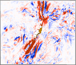For a given following current velocity $U$, these modulation effects are enhanced by larger value of $|\,f/\omega _0|$, i.e. larger rotational effect. This refraction effect is observed in our realistic MAB simulation (§3.2). Figure 10 shows a snapshot of mode-4 ITs, where one can see that the ITs are stretched, with longer wavelength and reduced amplitude, as they travel into the following current.

Figure 9.

Values of $k/k_0$ (Ł, blue), $E_n/E_{n0}$ (${---}$, red) for varying $\gamma$ at (a) $|\,f/\omega _0|=0.1$, (c) $|\,f/\omega _0|=0.6$, (e) $|\,f/\omega _0|=0.9$ and (g) $|\,f/\omega _0|=0.98$. Values of $|\mathcal {U}_n|/|\mathcal {U}_{n0}|$ (, red), $|\mathcal {V}_n|/|\mathcal {V}_{n0}|$ (, yellow), $|\mathcal {W}_n|/|\mathcal {W}_{n0}|$ (, blue), $|\mathcal {P}_n|/|\mathcal {P}_{n0}|$ (, red), $|\mathcal {B}_n|/|\mathcal {B}_{n0}|$ (, green) for varying $\gamma$ at (b) $|\,f/\omega _0|=0.1$, (d) $|\,f/\omega _0|=0.6$, ( f) $|\,f/\omega _0|=0.9$ and (h) $|\,f/\omega _0|=0.98$.

Figure 10.

The $M_2$-frequency meridional component of the mode-4 IT at an arbitrary phase, overlaid with vectors of the surface background (62 h averaged) velocity, showing the increase of the wavelength due to the following Gulf Stream, as highlighted by the black box.

For $\gamma <0$ (but not negative enough to trigger the singularity in (4.15)), i.e. IT propagates into an opposing current, we obtain $k>k_0$ (cf. figure 9a,c,e,g), meaning that the modal wavelength is shortened. The modal amplitudes of $\mathcal {W}_n, \mathcal {P}_n$ and $\mathcal {B}_n$ are amplified and $\mathcal {V}_n$ is suppressed (cf. figure 9(b,d, f,h). The modulations of $E_n$ and $\mathcal {U}_n$ are more complicated. It can be shown that there exists a threshold value of $|\,f/\omega _0| = \mathcal {F}^* \approx 0.958$, below which $E_n/E_{n0}$ and $|\mathcal {U}_n|/|\mathcal {U}_{n0}|$ increase monotonically with the increase of the opposing speed (cf. figure 9(a–f). For $|\,f/\omega _0| > \mathcal {F}^*$ (near-inertial waves), an anomaly occurs: $E_n/E_{n0}$ and $|\mathcal {U}_n|/|\mathcal {U}_{n0}|$ first decrease and then increase with the increase of the opposing velocity (cf. figure 9(g–h). The physical reason for this phenomenon can be elucidated using (4.8). As the modal IT propagates into the opposing current, the group velocity increases due to the refraction effect (cf. (4.7a,b)), which has the tendency to reduce $E_n$. For sufficiently large $|\,f/\omega _0|$ and small $|\gamma |$, this reduction of $E_n$ can exceed the amplification of $E_n$ due to both the increase of the opposing current velocity and the work done by radiation stress. This results in the decrease of $E_n$ in the opposing current, reflected by the decrease of the modal amplitude of $\mathcal {U}_n$. For $\omega _0$ at semidiurnal tidal frequency, the value of inertial frequency with $|\,f/\omega _0| = \mathcal {F}^*$ corresponds to the latitude of $67.4^\circ$ on Earth. These salient behaviours of ITs are distinct from those of the surface waves analysed in Longuet-Higgins & Stewart (Reference Longuet-Higgins and Stewart1961).

For $\gamma$ sufficiently negative, i.e. sufficiently large current opposing the IT, the solution of (4.15) can be singular, which indicates wave focusing. This occurs when $\gamma A + c_{p0}/c_p =0$, which can be solved to obtain the critical value of $\gamma ^*=-\sqrt {1/A}$. For $\gamma \leq \gamma ^*$, the opposing velocity can exceed the local modal group velocity of the IT, and the amplification of the modal energy becomes theoretically infinite due to energy accumulation. In practice, the modes of the IT are expected to break before this point is reached. Values of $\gamma ^*$ for different values of $|\,f/\omega _0|$ are plotted in figure 11, showing that the magnitude of the critical opposing velocity decreases as $|\,f/\omega _0|$ increases. For near-inertial waves with $f$ approaching $\omega _0$, the critical opposing velocity approaches zero. For $f$ close to zero, the modal velocity satisfies $c_g=c_p=c_n=c_{p0}$, and the magnitude of the critical opposing velocity reaches $c_{p0}$.

Figure 11.

Values of $\gamma ^*$ for different values of $|\,f/\omega _0|$.

While figures 9 and 11 apply to each mode of the IT separately, when combined, they describe the propagation of an IT that is a sum of vertical modes. For a given value of $f$ and thus $\gamma ^*$, since higher modes have smaller phase velocity $c_{p0}$, the critical opposing velocity to trigger wave focusing is smaller for higher modes than for lower modes. As the IT propagates into an opposing current, higher modes tend to break at smaller opposing velocity. Therefore, the opposing flow can block the higher modes, and allow the lower modes to pass through (this is in principle similar to the blockage effect of surface waves described in Shyu & Phillips Reference Shyu and Phillips1990). This analysis is consistent with the observation of long-distance propagation of low-mode IT in the ocean, although the IT dynamics in the general case is incomparably more complicated.