1 Introduction
A classifier ensemble is a group of classifiers whose individual decisions are merged in some manner to provide, as an output, a consensus decision. The overarching aim of this approach is to combine outputs of a number of models, also referred to as base classifiers, to generate a single aggregated output that outperforms any of the base classifiers in isolation. The first stage in the process of generating a classifier ensemble is the generation of a collection of base classifiers. One approach is to apply N different learning methods, with a single training data set, to obtain N different classification models. An alternative approach is to create N different portions of data from the training data set and employ a single learning algorithm with each portion. During the learning phase, it is important to adopt an approach that allows the creation of diverse classifiers. It has also been shown that the appropriate selection of base classifiers, rather than simply combining all of them in one single ensemble, may impact upon the final overall classification accuracy (Ruta & Gabrys, Reference Ruta and Gabrys2005; Saeedian & Beigy, Reference Saeedian and Beigy2009). Base classifier selection may be performed in either a static or dynamic manner. In the static approach, the same subset of base classifiers that are selected is applied for all testing samples. In the dynamic approach, selection is performed for each new instance individually.
After obtaining a collection of base classifiers, the next step is to combine their outputs in order to obtain the final decision. During this phase, the main issues to be considered are related to what types of information are going to be combined and which combination method is going to be applied. For an unseen pattern, all base classifiers make their decisions, which subsequently form the input to a combination function. Different methods of combination use different types of base classifier outputs, for example class label or class probability distribution may be used. An alternative approach is to use predictions as a set of attributes to train a combination function in terms of meta-learning (Ting & Witten, Reference Ting and Witten1997).
Combining classifiers and hence the creation of classifier ensembles has been proposed by many studies as a method of improving the performance of a single classifier (Dzeroski & Zenko, Reference Dzeroski and Zenko2004; Bi et al., 2008; Machova & Barcak, Reference Machova and Barcak2006; Danesh et al., Reference Danesh, Moshiri and Fatemi2007; Jurek et al., Reference Jurek, Bi, Wu and Nugent2011). It has already been presented that this approach has the ability to provide better results than applying the single best classifier to the same problem (Danesh et al., Reference Danesh, Moshiri and Fatemi2007). The key to producing the most successful ensemble method can be viewed as an approach that requires applying both, an appropriate combination method in addition to the careful selection of the base classifiers.
In summary, the main goal of designing a classifier ensemble is to obtain the best possible classification accuracy. This area of research has attracted significant interest in recent years. The work presented by Rokach (Reference Rokach2010) considers related work in this field and has been presented in the form of a tutorial, which describes the taxonomy for characterizing ensemble methods and the general process of constructing classifier ensembles, including the key challenges such as: ensemble framework and generation, combination methods, diversity generation, ensemble selection and multi-strategy ensemble learning. In this paper, we have addressed the most important issues in the domain of classifier ensembles; however, it has been the aim of this paper to provide a state of the art review of the most well-known ensemble techniques and to trace the recent attempts, which have been made to improve their performance. Within this paper, we present and compare an updated view on the different modifications of bagging, boosting and stacking, which have been made to these techniques to address some of the drawbacks of the methods namely the low diversity problem in bagging and the over-fitting problem in boosting. We review a number of classifier ensemble selection methods based on both static and dynamic approaches. We demonstrate how different selection criteria namely accuracy, diversity or their combination have been applied to improve the final performance of the ensemble. In addition, we present in the paper some new directions, which have been adopted in the area of classifier ensembles from a range of recently published studies. It is anticipated that the paper will provide a survey of the most well-known ensemble techniques, challenges and trends within these areas and can help others to understand the ensemble process with the aim of stimulating new ideas and new directions in the area of generating classifier ensembles.
The remainder of the paper is organized as follows. Section 2 presents the theoretical framework of classifier ensembles. Section 3 reviews different learning approaches to generation of base classifiers with a focus on different variants of bagging and boosting. In Section 4, we describe different ways of combining outputs of base classifiers. The problem of ensemble selection is introduced in Section 5, followed by the summary of the paper.
2 Theoretical framework
The main idea of combining classifiers is to build an ensemble that will be more effective than any of its individual members operating in isolation. One of the simplest representations of an ensemble framework has been presented in Figure 1.
An example of the representation of a simple ensemble method

In this case, each base classifier is generated by a different learning method and the same training set. The final ensemble output is presented as a weighted average of the outputs of the base classifiers. The weight of each classifier represents its contribution to the final decision. In the simplest case, all weights are made equal to 1. A multitude of investigations have previously demonstrated that the combination of different classifiers can improve the final prediction of the member classifiers (Garcia-Pedrajas, Reference Garcia-Pedrajas2009; Parvin & Alizadeh, Reference Parvin and Alizadeh2011). Hansen and Salamon (Reference Hansen and Salamon1990) showed that for an ensemble of artificial neural networks (ANN), if the accuracy of each model is >0.5 and if their responses are independent, then the larger the number of networks in the ensemble, the smaller the chances of an error by majority voting (MV).
A widely used concept for analyzing supervised learning algorithms is referred to as a noise, bias and variance decomposition of error (Webb & Conilione, Reference Webb and Conilione2003). According to this analysis, the error of a learning algorithm can be decomposed into three aspects namely: noise, bias and variance. These aspects are derived with reference to the performance of a model when trained with different training data. Noise is a measure of an error incurred independently of the learning algorithm, for example class or attribute noise in data. Bias for a particular input is a measure of an average error of the learner trained with different training sets. Variance is a measure of how much the learner's predictions differ as it is applied with different learning data. In other words, it is a measure of sensitivity of the learning algorithm to the training set. A number of different mathematical definitions of bias and variance for classification problem have been proposed (Hansen, Reference Hansen2000). Some widely employed approaches to estimating bias and variance from data are referred to as a holdout approach (Kohavi & Wopert, 1996) or multiple fold cross-validation (Webb, Reference Webb2000). It has been presented that there is a trade-off between bias and variance of classification models (Hansen, Reference Hansen2000). Simple classifiers tend to have large bias and small variance. When the complexity of model increases, the bias becomes smaller, whereas the variance becomes larger. It has been investigated that some ensemble methods can significantly reduce bias and/or variance (Bauer & Kohavi, Reference Bauer and Kohavi1999) of learning algorithms. For example, it has been presented that an ensemble technique referred to as bagging can reduce variance (Valentini, Reference Valentini2004, Reference Valentini2005), therefore it is successful while applied with unstable learners like decision trees (Dietterich, Reference Dietterich2000) or neural networks (Maclin, Reference Maclin1997). It has been presented that another ensemble method, referred to as boosting, can reduce bias and variance, which makes it more effective while applied with some weak learners like decision stumps (Rodríguez & Maudes, Reference Rodríguez and Maudes2008).
In their work, Krogh and Vedelsby (Reference Krogh and Vedelsby1995) presented the generalization error, which expresses the relation between variance and bias in an ensemble under instances of continuous outputs as follows:
 $$E\, = \,\overline{E} {\rm{ - }}\overline{A} $$
where  $$\[--><$>\overline{E} <$><!--$$
represents the weighted average of the errors of the individual ANNs over the input distribution. The error of an individual classifier Ci on instance x is calculated as
 $$\[--><$>{{e}_i}(x)\, = \,{{({{C}_i}(x){\rm{ - }}{{y}_i})}^{\rm{2}}} <$><!--$$
.
 $$\[--><$>\overline{A} <$><!--$$
represents the weighted average of the ambiguities of the individual networks over the input distribution where the ambiguity of a single classifier on input x is defined as the variance of the classifier around the weighted mean
 $$\[--><$>{{a}_i}(x)\, = \,{{({{C}_i}(x){\rm{ - }}C(x))}^{\rm{2}}} <$><!--$$
. The weighted average of ambiguities measures the disagreement among models. Zenobi and Cunningham (Reference Zenobi and Cunningham2001) proposed a measure of ambiguity; hence, Equation (1) would also hold for a classification problem. Considering that for classification problems the most frequently used error measure is the 0–1 loss function, they suggested a measure of ambiguity as presented in the following equation:
 $${{a}_i}(x)\, = \,\left\{ \matrix{ \matrix {\rm{0}} & {{\rm{if}}} \quad {{{C}_i}(x)\, = \,C(x)} \\\end{} \cr\matrix {\rm{1}} & {{\rm{otherwise}}} \hfill\\\end{} \\ \end{} \right$$
From Equation (2) we can see that if the ambiguity is very small the ensemble error will almost be equal to the weighted average of its individual members. We can also see that the ensemble error is always smaller than the average of the individual classifier errors. The conclusion from this work demonstrated that apart from obtaining accurate base classifiers, it is important that they disagree as much as possible. We say that two classifiers disagree if they make mistakes on different groups of instances. By an accurate classifier, we mean the classifier that provides better accuracy in comparison with a random guess. In the same work, Zenobi and Cunningham investigated that finding the optimal weights (α 1, …, αT) for individual classifiers, rather than using the same weights for all of them, can significantly improve the performance of the ensemble.
Schapire et al. (Reference Schapire, Freund, Bartlett and Lee1998) introduced the concept of the classification margin to analyze the behaviors of multiple classifiers. They defined the margin of an instance as the difference between the support given to the correct class and the highest support given to any of the incorrect classes. Let vi,y be the output from classifier Ci for class y. We can calculate the margin of the ensemble on instance (xk, yk) as presented in the following equation:
 $$\overline{m} \, = \,\mathop{\sum}\limits_{i\, = \,{\rm{1}}}^T {{{\alpha }_i}{{m}_i}} $$
where  $$\[--><$>{{m}_i}\, = \,{{\nu }_{i,{{y}_k}}}{\rm{ - }}{\mathop{{\max }}\limits_{{j\, \ne \,k}}} {{\nu }_{i,{{y}_j}}}<$><!--$$
is the margin of a single classifier. One can notice that a margin is a value from the interval of [−1, 1] where the high margin is interpreted as a confident classification. From their observations, it was found that two ensemble methods, bagging and boosting, tended to increase the margin associated with the instances. In addition, it was demonstrated that the generalization error of the ensemble can be improved if we try to increase the margin of the ensemble on training data.
Dietterich (Reference Dietterich2000) in his work presented three reasons why it is often possible to generate a very good ensemble. These were categorised as being statistical, computational and representational. From a statistical point of view, by constructing an ensemble from a small number of classifiers, their votes can be averaged to decrease the risk of selecting the wrong classifiers, from which a decision is to be made. From a computational point of view, if a learning algorithm works by performing a local search it may become stuck in a local optima. An ensemble generated by performing a local search starting from a range of different points can provide an improved approximation compared with an individual classifier. The third reason described by Dietterich was representational. We can consider learning algorithms as a searching space of hypotheses (classifiers) to locate the true classification function. In many machine learning applications, the hypotheses spaces searched are finite and do not contain the true hypotheses. This is caused by applying a finite range of training samples. By calculating the weighted sums of hypotheses, it is possible to expand the space hence increasing the chances for locating the true function. Dietterich confirmed that the key for a successful ensemble method is to generate base classifiers that have an accuracy rate above 0.5 and do not misclassify the same group of instances.
The final problem is referred to as the diversity of base classifiers and has been widely studied in the past. Very often diversity (Melville & Mooney, Reference Melville and Mooney2003; Kuncheva & Whitaker, Reference Kuncheva and Whitaker2003) was considered, following the criteria of individual accuracy, as a criterion for selecting a pool of base classifiers. According to previous research (Hu, Reference Hu2001), diversified models provide uncorrelated decisions, which lead to a more accurate ensemble. Kuncheva and Whitaker (Reference Kuncheva and Whitaker2003) presented 10 different diversity measures. The measures can be pair wise, for example Q statistic and correlation or non-pair wise, for example, entropy and variance. According to the experimental results, all the measures significantly improved the performance of MV. Different techniques such as applying disparate feature subsets (Bryll et al., Reference Bryll, Gutierrez-Osuna and Quek2003), different training sets obtained by clustering (Gan & Xiao, Reference Gan and Xiao2009) and random selection (Breiman, Reference Breiman1996), have been suggested to increase diversity.
3 Ensemble generation
The first stage when building a classifier ensemble involves the process of obtaining a set of different base classifiers. One approach, which may be adopted, is to use a group of N different learning methods (Kittler et al., Reference Kittler, Hatef and Duin1998). In this approach, each base classifier is built using the same training data set and a different learning algorithm. As a result, a number of N different classification models are obtained. The ensuing step is to combine their outputs to provide a final consensus decision. Different approaches that have been adopted for the purposes of combination are described in Section 4.
The second approach, which may be adopted in the process of building a set of base classifiers, relates to the use of a single learning method and different training sets (Dietterich, Reference Dietterich2000). The main issue with this approach is the conversion of the original data set in an efficient manner to obtain a collection of different training data sets. In some techniques, the original data set is divided into N subsets by random selection or clustering. Another approach involves the manipulation of the distribution of the data. Following the creation of the subsets, each base classifier is built using the different subsets and the same learning algorithm. The following sections describe and compare the most popular techniques, based on this approach, which have been investigated.
3.1 Partitioning of the training data set
The most popular technique of obtaining different training sets from a single data set is referred to as bagging. Fundamentally, bagging relates to the approach where the training sets are randomly chosen k times with replacement (bootstrap techniques) from the original data set (Breiman, Reference Breiman1996). With this approach, it is possible that some instances may appear more than once in some of the training sets and some instances may not be present at all. As a result, k training sets (and subsequently k different classifiers), with a size equal to the original set of data, are obtained. The main advantage of bagging is that the individual ensemble members can be independently trained in parallel, which reduces the time required for training. Figure 2 depicts the pseudo-code of the bagging algorithm.
Pseudo-code of bagging algorithm
The disadvantage with bagging is that training subsets generated by random selection with replacement are not totally independent. It has already been noticed that bagging can only improve performance of unstable classifiers (Breiman, Reference Breiman1996), for example decision trees (Dietterich, Reference Dietterich2000) or ANN (Maclin, Reference Maclin1997). These are models that are very sensitive with respect to the small changes in the training data. The reason for this is that in the bagging approach, only unstable learning methods can obtain diverse base classifiers (Breiman, Reference Breiman1996). In the study of Machova and Barcak (Reference Machova and Barcak2006), bagging was applied with binary decision trees to generate base classifiers. Experimental results demonstrated that the minimum number of base classifiers required to obtain the same efficiency as a perfect decision tree, could be found. In this particular case, bagging obtained the best performance when the number of base classifiers was >20.
In the study by Skurichina et al. (Reference Skurichina, Kuncheva and Duin2002), it was suggested that the instability of the model, measured on training data, could be used to predict the accuracy of the bagging technique. It was also shown by Skurichina and Duin (Reference Skurichina and Duin1998), that bagging did not improve the accuracy of stable classifiers. In their work, a modification referred to as ‘nice bagging’ was introduced. In this method, only the bootstrap version of the base classifiers, which perform better than the original model (built with all training data), are included in the ensemble. Although this approach did not improve the bagged model in terms of accuracy, it did improve the stability of the final model.
It has been reported that a support vector machine (SVM) may not be expected to be significantly improved by the bagging technique, due to its stability and high accuracy (Buciu et al., Reference Buciu, Kotropoulos and Pitas2006). In the study by Wang and Lin (Reference Wang and Lin2007), it was proposed to consider bagging for a class-wise expert based on an SVM framework (CeBag). These are classifiers that perform very well with instances from one class and relatively poorly with instances from different classes. For each bootstrap sample, three models were trained: positive and negative wise-class experts together with a mediator classifier. The mediator classifier was responsible for the samples on which the first two experts disagreed. No theoretical analysis was conducted, however, the results demonstrated that the modified version of bagging can be successfully applied in order to improve the performance of the SVM classifier. The proposed method outperformed a single SVM and Bagging SVM in most of the data sets considered. The reason for these results may be related to the increased diversity among the SVM models, taking into account that they focused on different aspects of the samples during the learning phase.
The use of bagging with the nearest neighbor classifier (kNN) (Breiman, Reference Breiman1996) has also been reported as offering optimization challenges. In the work reported by Zhou and Yu (Reference Zhou and Yu2005), bagging was adapted to kNN classifiers by applying randomness to distance metrics. This proposed variant of bagging was referred to as BagInRand. A new distance metric with two parameters, referred to as Minkovdm, was developed by combining value difference metric (VDM) (categorical attributes) (Stanfill & Waltz, Reference Stanfill and Waltz1986) and Minkowsky distance (continuous attributes):
 $${ Minkovd{{m}_{p,q}}({{x}_{\rm{1}}},{{x}_{\rm{2}}}) & \, = \,\left( {VD{{M}_q}({{x}_{{\rm{11}}}},{{x}_{{\rm{21}}}})\, + \, \ldots \, + \,VD{{M}_q}({{x}_{{\rm{1}}j}},{{x}_{{\rm{2}}j}})\, + \,} \right. \cr & {{\left. {{{{\left| {{{x}_{1,\,j\, + \,{\rm{1}}}}{\rm{ - }}{{x}_{2,\,j\, + \,{\rm{1}}}}} \right|}}^p} \, + \, \ldots \, + \,{{{\left| {{{x}_{{\rm{1}},d}}{\rm{ - }}{{x}_{{\rm{2}},d}}} \right|}}^p} } \right)}^{{\rm{1}}/p}} \cr}$$
where x 1 and x 2 are instances represented by d-dimensional vectors: (x 11, …, x 1d) and (x 21, …, x 2d). VDMq (x 1i, x 2i) is the distance between the values of x 1 and x 2 on attribute i. The distance between values w and v on attribute a is computed as
 $$VD{{M}_q}(v,w)\, = \,{{\mathop{\sum}\limits_{c\, = \,{\rm{1}}}^C {\left| {\frac{{{{N}_{a,v,c}}}}{{{{N}_{a,v}}}}{\rm{ - }}\frac{{{{N}_{a,u,c}}}}{{{{N}_{a,u}}}}} \right|} }^q} $$
Na ,v stands for the number of training instances with value v for attribute a. Na ,v ,c denotes the number of training instances from class c with the value v on attribute a and C is the number of classes. The original data set was first bootstrap sampled. Then, for each sample, random values were assigned to the parameters p and q. In this way, each kNN was generated not only with a different training set but also with a different distance metric. Application of the Minkovdm metric to obtain different kNN classifiers did not bring significant improvement over single kNNs. Nevertheless, combination of both: bagging and Minkovdm was reported as offering improved performance in comparison with the single model.
A different modification of bagging referred to as Double-Bagging was introduced by Hothorn and Lausen (Reference Hothorn and Lausen2003). In this approach, the observations that were not part of the bootstrap sample (out-of-bag), were used to train a second classifier. For each bootstrapping step, the out-of-bag sample was used to perform a linear discriminate analysis. The discriminate variables of each bootstrap sample were incorporated as supplementary predictors for the classification tree. One of the advantages with this approach was that the coefficients of the discriminate function were estimated by an independent set of variables. This helped to avoid over-fitted discriminate variables in the tree growing process. The best classifiers studied in the problem, were improved by Double-Bagging in several experiments. A number of the examples investigated demonstrated that this modified version of bagging can provide better performance than the standard one.
A further drawback of bagging, in addition to low diversity, is the large amount of resources required to both store and learn the group of base classifiers. A number of solutions have been proposed, which aim to minimize both of these problems (Estruch et al., Reference Estruch, Ferri, Hernández-Orallo and Ramírez-Quintana2004). The optimization technique developed was based on sharing the joint parts of the models from an ensemble formed by decision trees. For each bootstrap sample a new classifier was built by continuing the construction of the multi-tree (BagMTD). Only nodes that were not considered in the previous iterations were used. In other words, the multi-tree was a single structure containing an ensemble of decision trees that were obtained by bagging, without reusing their joint parts. The training time was significantly reduced while using the multi-tree approach, without loss of classification accuracy.
Zeng et al. (Reference Zeng, Chao and Wong2010) presented that bagging can be improved if only the optimal models from all those generated are selected as base classifiers. The new SBCB (Selecting Base Classifiers on Bagging) algorithm improved a bagging algorithm by applying an optimization process to select the optimal base models according to the diversity and accuracy. First, similar to the process of bagging, a collection of classifiers was built with different bootstrap samples. Then all models were used to classify instances from a given set and those with accuracy lower than 50% were eliminated from the ensemble. Following this the Entropy Measure was applied to select the group of classifiers with the highest diversity. The remaining group of classifiers was considered to comprise the final ensemble. A voting rule was used to combine the predictions from each of the classifiers. The experimental results demonstrated that the proposed SBCB algorithm had the ability to improve the performance of generic bagging.
Given that bagging is a technique of generating diverse classifier ensembles through the manipulation of training data sets, its accuracy may be affected by some characteristics of the training data themselves. For example, it was noticed that the noise inherited in the training data could be used for increasing diversity in the bagging technique proposed by Dietterich (Reference Dietterich2000). In the study by Skurichina et al. (Reference Skurichina, Kuncheva and Duin2002), it has been shown that bagging is mainly effective with a small training sample size, when the number of training instances and dimensionality of the data are comparable. In the same work it was shown that for bagging the diversity (Q statistic) decreases when the training sample size increases.
A variant of bagging, referred to as Wagging (Weights Aggregation), was proposed by Bauer and Kohavi (Reference Bauer and Kohavi1999). Similar to the process adopted in bagging, the training data set was repeatedly perturbed, as an alternative to sampling from it. For the weighting process, Gaussian noise with a given standard deviation and zero mean was added to each weight. At the beginning all instances were uniformly weighted. Noise was added to the weights of the instances in each iteration of the process, and then one classifier was induced.
In the work of Datta and Pihur (Reference Datta and Pihur2010), a novel ensemble classifier generated by a combination of bagging and rank aggregation was proposed. The approach was very similar to the original bagging method, with the difference that instead of one classifier, there were a number of classifiers trained with each bootstrap sample. Following this, each model was used to predict class labels on a group of instances that were not included within the bootstrap sample. A range of performance measures were applied to evaluate the performance of each classifier. The rank aggregation procedure was then used to determine the best performing classifier. As a result, for each bootstrap sample, only one model was selected to be included into the final ensemble. The final decision was calculated by the MV method. Eight individual classifiers were used in the experiments. For all data sets considered, the ensemble obtained a result equal to, or better than the best individual classifier. There was, however, one significant drawback of the proposed approach, which was computational time. Comparing with the original process of bagging, a number of classifiers were trained with each bootstrap sample as opposed to one only. In addition to this, the rank aggregation may also take considerable time if there are a large number of models generated within each iteration.
A method that involved the use of clustering during the pre-processing phase was introduced by Gan and Xiao (Reference Gan and Xiao2009). In that work, each model was trained with a subset of the original training data set. This approach differed from bagging, given that instances were divided according to their features, not by random selection. An improved K-Means algorithm was used to generate a number of different sample subsets. ANNs were used as the base classifier. Each model was trained with one of the clusters and the ensemble was in this instance comprised all the ANNs. The proposed method was compared with bagging and boosting. In all the experiments, the prediction error of the proposed ANN-based ensemble was smaller than the bagging or boosting ANN-based ensemble. We can postulate from this study that clustering may be a more effective way of obtaining different training sets than random selection or data distribution modification. The reason for this could be speculated that the base models are trained on different regions of data and as a result they become local experts. We can speculate that by training base classifiers in this manner, the diversity of the final ensemble can be increased.
3.2 Manipulation of data distribution
An alternative technique, which applies different training data sets and the same learning method, is referred to as boosting (Freund & Schapire, Reference Freund and Schapire1999). Boosting is an iterative approach where the distribution of the training set is dynamically altered, based on the classifier's accuracy. After each base classifier is built and added to the ensemble, all instances are reweighted: those that have been correctly or incorrectly classified loose or gain weight, respectively. The final prediction is made by taking a weighted vote of each base classifier's prediction. The weights are proportional to the accuracy of each classifier relative to its training set. A very effective and well-known boosting method is AdaBoost, introduced by Freund and Schapire (Reference Freund and Schapire1999). The AdaBost algorithm is presented in Figure 3.
The Boosting algorithm AdaBoost
We can notice that unlike bagging, with boosting base classifiers cannot be trained in parallel given that the inputs of one model depend on outputs of others. This has the effect of extending the training time of the ensemble. It has been demonstrated that AdaBoost can improve the accuracy of single classification models such as decision trees (Rodríguez & Maudes, Reference Rodríguez and Maudes2008) or ANNs (Schwenk & Bengio, Reference Schwenk and Bengio2000).
In the bagging method, the biggest drawback is related to the low diversity among the base classifiers. For boosting this problem decreases given that a larger change in the training data can be obtained using this technique. Despite this fact, in many studies it was considered how the performance of boosting applied with stable models can be improved by increasing the diversity of base classifiers. In the work of He et al. (Reference He, Song, Shen and Hai2010), boosting was applied to improve the accuracy of kNN classifiers (Bs-kNN). They modified the original approach by introducing attribute selection into the process of training base classifiers. This resulted in each model being built with different data samples and a different subset of features. In each iteration, they applied the set of features that produced the highest performance gain. The empirical study demonstrated that the improvement of kNN was statistically significant.
An algorithm referred to as Adaptive Graphe-Based K-Nearest Neighbor (A-kNN) was proposed in the work of Murrugarra-Llerena and Lopes (Reference Murrugarra-Llerena and Lopes2011). The idea was to improve the kNN algorithm in the manner of mapping the boosting technique into a graph-based approach. Initially, a kNN network based on the similarity between instances (vertices) was built using the training data, where k was a set value. In other words, each instance was linked with its k nearest neighbors. Next, all instances from the training set were classified using the current network. In the ensuing iterations, the number of links of each vertex (degree of vertex) was modified similar to the example distribution within the AdaBoost algorithm. The number of links was increased for the misclassified examples. The maximum value of k was predefined from the outset. The degree of each instance was increased until the example was correctly classified or the maximum value of k was reached. In the classification phase, for the unseen instance, its closest neighbor is selected from the training set. Based on the number of edges (k) of the closest neighbor, the unseen pattern was classified based on the class labels of its k closest neighbors. In an empirical study, the A-kNN approach was compared with a range of other classifiers: Naive Bayes, SVM, C4.5, single kNN and ensembles (boosting) of those classifiers. The proposed method performed as well or better than the other methods.
Two different improved methods of boosting kNN classifiers were proposed in the work of García-Pedrajas and Ortiz-Boyer (Reference García-Pedrajas and Ortiz-Boyer2009). In the proposed approach, the input space was modified by the means of input selection (kNN.NsRSM) or nonlinear projection (kNN.BSP). In kNN.NsRSM different subspaces, that minimized the weighted error, were selected for each kNN classifier. In other words, a new subset of inputs, relevant to the distribution of the instances, was obtained to train each base classifier. In kNN.BSP, the nonlinear projection was constructed using weight vectors (distribution of the training set) that were obtained using a boosting method. Similar to the previous approach, it aimed to minimize the weighted error for each boosting step. The intention in both of the scenarios was to introduce a level of instability into the kNN learning method through a process of input space modification. A more instable learning method was meant to provide a higher diversity among the base classifiers to be obtained. It appeared that the idea was successful, given that both methods: kNN.NsRSM and kNN.BSP improved performance in comparison with a single kNN model.
A number of studies have been performed with the aim of considering how the AdaBoost technique can be improved in terms of accuracy and efficiency. A variant of the AdaBoost (r-AdaBoost) algorithm was proposed in the study by Rodríguez and Maudes (Reference Rodríguez and Maudes2008). In this case, weak decision trees (stumps) were used as the base classifiers. The concept of the proposed method was to improve the performance of the final ensemble by applying more complex weak models. The approach was based on combining several stumps into a more complex tree without increasing the computational complexity or memory requirements. The parameter r was considered as a level of reuse and it determined the number of classifiers from the former iterations that were going to be used. In other words, rather than applying a single model that was generated in an iteration of AdaBoost, it was combined with r previous classifiers. The concept in the reuse variant of AdaBoost was to combine several weak models into what may be perceived as a not so weak model in an effort to obtain an improved final ensemble. Given that combining models from previous iterations decreases diversity of the models, only two levels of reuse were applied: r = 1 and r = 2. The method improved the classification accuracy of the AdaBoost approach. A similar improvement in performance was not, however, witnessed with more complex decision trees. This approach could be applied with other classification methods, however, it will not be useful with those that generate strong base classifiers.
A different variant of the AdaBoost method (P-AdaBoost), based on the parallel approach, was proposed by Merler et al. (Reference Merler, Capriel and Furlanello2007). In this approach, weights assigned to the instances were estimated from those obtained in the standard AdaBoost process. In the first step, the AdaBoost algorithm was run for a finite number of iterations and all weight vectors were recorded. In the following step, distribution of each data point was estimated from its weight's evaluation. For each base classifier, new values of the weights were assigned randomly, by sampling the respective distribution. The advantage of this technique was a reduced number of iterations compared with the original AdaBoost method. Manipulation of the number of iterations in the first phase allowed control of the computational cost, however, it did not change the number of base classifiers inducted.
Boosting methods, compared with bagging methods, were reported to perform much worse after adding noise to the data (Dietterich, Reference Dietterich2000). In addition, they have been reported as being ineffective when applied with a strong learner (Wickramaratna et al., Reference Wickramaratna, Holden and Buxton2001). Strong models are capable of correctly classifying most of the samples from the training set in the initial first few iterations. As a consequence, weights of a number of difficult instances and outliers become very large and are the main causes to the over-fitting problem; hence, resulting in producing a low accurate outcome. Some additional improvements to boosting methods have been proposed to avoid this known problem.
An SVM is one of the classifiers that cannot usually be considered in conjunction with boosting. A modified version of AdaBoost, referred to as AdaBoostSVM, has nonetheless been investigated by Li et al. (Reference Li, Wang and Sung2005). A set of SVM classifiers with a Radial Basis Function kernel (Schölkopf et al., Reference Schölkopf, Sung, Burges, Girosi, Niyogi and Poggio1997) was generated for AdaBoost by adjusting the kernel parameter instead of using a fixed one. This approach aimed to generate a collection of not very strong classifiers in an effort to avoid the over-fitting problem. The proposed method outperformed AdaBoost with ANNs as base classifiers. Besides this, AdaBoostSVM appeared to work better than a single SVM when applied with unbalanced data. Additionally, in the same work, an improvement based on increasing diversity was proposed (Diverse AdaBoostSVM). The degree of diversity was calculated in each cycle (Melville & Mooney, Reference Melville and Mooney2003). If the degree of diversity value was higher than the predefined threshold the classifier was selected.
A similar SVM weakening strategy, based on adjusting the kernel value, was applied in the work of Wang and Lin (Reference Wang and Lin2007). This approach adopted a new weighting rule that separates instances not only according to classification results but also regarding to the distance from the separating hyper plane. The aim of the approach was to prevent the highlighting of difficult instances or outliers, which usually cause the over-fitting problem.
A boosting technique, referred to as MadaBoost, was proposed by Domingo and Watanabe (Reference Domingo and Watanabe2000). Similar to the previous method reported by Wang and Lin, the aim of the work was to avoid the over-fitting problem through modification of the AdaBoost weighting system. In this case, weights assigned to the instances were bounded by each example's initial probability. This approach aimed to control the growth of the weights and to prevent them from becoming arbitrarily large.
Different solutions that help to avoid the over-fitting problem and improve accuracy in the boosting methods were investigated by Vezhnevets and Barinova (Reference Vezhnevets and Barinova2007). The concept considered was to remove confusing instances from the training data and train AdaBoost with the resulting data. Confusing samples were considered as those that were not correctly classified by a ‘perfect’ Bayesian model. The proposed solution assisted in avoiding the over-fitting problem and reduced classification error.
A derivative of AdaBoost, referred to as Local Boosting, was presented in the study by Zhang and Zhang (Reference Zhang and Zhang2008). The concept was to calculate a local error of each training instance in each cycle and based on this value assign a probability that the instance was going to contribute to the next classifier's learning process. In AdaBoost, weights of all misclassified samples are increased automatically in each iteration. In Local Boosting, the aim was to initially identify all noisy instances that should not be a part of the next base model's learning set. Each misclassified sample was initially compared with its neighborhood. If similar instances had been misclassified, the weight was subsequently increased. If they had been correctly classified, the sample was considered as noise and its weight was subsequently decreased. The proposed approach was found to be more accurate and robust to classification noise compared with AdaBoost.
An approach similar to boosting and bagging, referred to as MultiBoosting was presented by Webb (Reference Webb2000). This approach considered a combination of wagging and boosting. In MultiBoosting base classifiers are generated similar to the process with AdaBoost with the main difference that the weights of the instances are drawn from the Poisson distribution. It was proved by work presented by Webb (Reference Webb2000) in a number of experiments that this technique obtained better mean results than any bagging or AdaBoost decision trees.
3.3 Partitioning the attribute space
Another approach to generating a collection of base classifiers with the same training data set is by applying different feature subspaces. A well-known technique that applies random subspaces to generate ensemble members is referred to as Random Forest (Breiman, Reference Breiman2001). A Random Forest is a classifier ensemble composed of a large number of individual trees. Individual trees are generated similarly as in the bagging process. The input parameters are the size of the ensemble and the number of variables that are used to determine the split at a node of the trees. Each tree is built with one bootstrap sample. For each node, variables that are used to determine the decision are randomly selected. Following the generation of a group of tress, a voting method is applied to generate the final decision. To a certain extent, the Random Forest may be considered as being a variant of the bagging technique. It was demonstrated (Breiman, Reference Breiman2001) that Random Forest performs competitively to boosting and bagging.
A method referred to as Attribute Bagging was proposed in the study by Bryll et al. (Reference Bryll, Gutierrez-Osuna and Quek2003). In this approach, to increase diversity, as opposed to subsets of instances, subsets of attributes were randomly chosen. Different numbers of attributes were investigated and selection did not include replacement. M selected feature subspaces were ranked according to their accuracy on the training data, with only the best k out of M being applied. Based on the analysis performed, it was apparent that such a modification of the bagging technique had the ability to provide better results in both accuracy and stability.
Another method considered for obtaining sets of different base classifiers by subspace selection was presented by Li and Hao (Reference Li and Hao2009). The concept introduced was similar to the process introduced in Attribute Bagging (Bryll et al., Reference Bryll, Gutierrez-Osuna and Quek2003). It involved the training of the classifiers on a different subset of features to obtain a higher level of diversity. In this approach, each feature was considered as one dimension in the Euclidean space. The approach adopted the random Oracle classifier to generate a hyper plane H that split the Euclidean space into two subspaces Ω+ and Ω−. One NB classifier was built in each of the subspaces. The final ensemble consisted of all generated models. The proposed method resulted in being the more successful compared with the bagging or boosting approach when evaluated on a number of data sets.
A method of creating a 1ANN ensemble using feature selection and multiple distance functions (DF-TS-1NN) was proposed by Tahir and Smith (Reference Tahir and Smith2010). The aim was to generate an ensemble where each member uses a different set of features and a different distance function. This approach was meant to reduce the probability that errors of individual classifiers are correlated. Feature selection was performed by application of the Tabu Search algorithm (Sait & Youssef, Reference Sait and Youssef1999). Five different distance measures were used within the 1ANN models. Following evaluation, the proposed technique not only improved single classifier performance, however, the approach significantly outperformed classifiers such as: Bagging C4.5, Bagging 1NN, AdaBoost C4.5 and AdaBoost 1NN.
3.4 Summary
For all of the methods based on obtaining a collection of base classifiers using different training data and the same learning method, there are two key issues, which should be considered. First, the technique of dividing the original training data set into subsets should be considered. Second, the selection of the learning method for training base classifiers should be considered. These two problems appear to be very connected with each other. For example, if subsets of training data are not different enough, only unstable learning methods can obtain diverse classifiers (Breiman, Reference Breiman1996). Bagging and boosting are not very efficient when applied with stable learning methods. Usually, some improvement has to be undertaken to obtain diverse base classifiers. Attribute partitioning may be viewed as an effective way for generating good ensembles that do not rely on stability. Another parameter, which may be viewed as a drawback of the methods, introduced in this Section is complexity. Usually, a large number of base classifiers have to be generated to obtain a good ensemble.
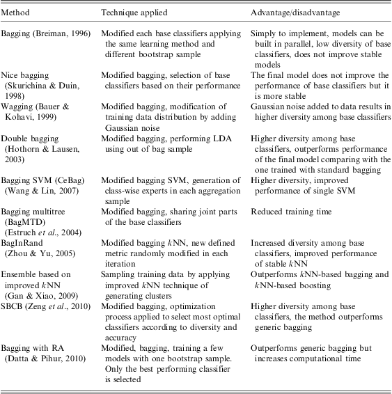
In an effort to provide an improved overview of the approaches of bagging and boosting, which have been considered in addition to their evaluations, Tables 1–3 aim to summarize all of the aforementioned methods. From the summary presented in Table 1, we can gain an appreciation that the majority of the work that has been undertaken has been carried out with respect to bagging and with the trend focussing on increasing the diversity among base classifiers.
Summary of methods based on partitioning of training data set
SVM = support vector machine; SBCB = selecting base classifiers on bagging.
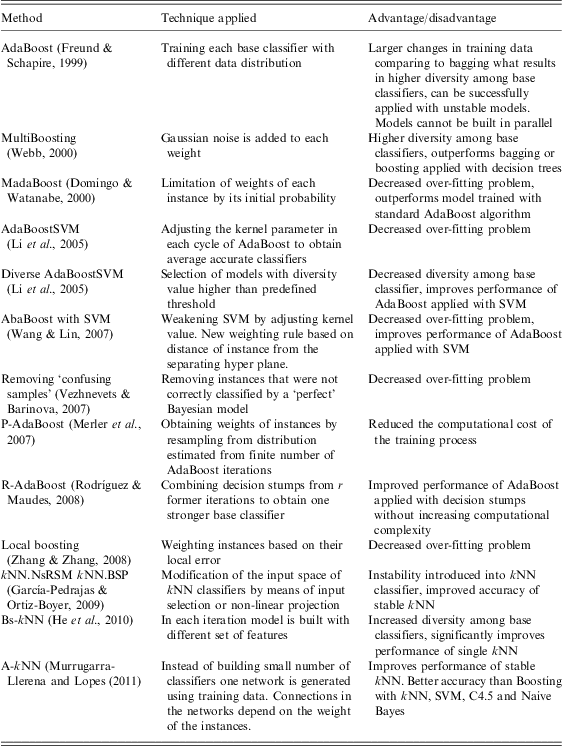
Table 2 presents a summary of the research conducted within the area of boosting methods as described in the previous sections. We can observe that the biggest problem with this approach is the low resistance to noise in the data, especially when strong and stable models are applied as base classifiers. There have been, however, a number of successful approaches proposed to address these issues.
Summary of boosting methods and proposed attempts for improvements
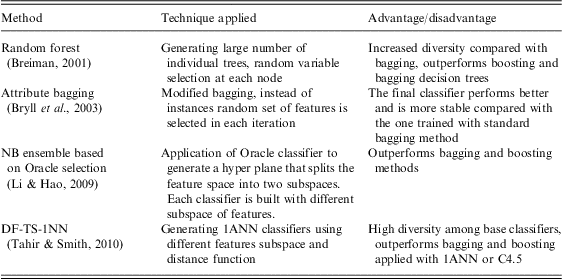
Table 3 presents a summary of the methods that apply partitioning of the attribute space to obtain diverse base classifiers.
Summary of methods based on partitioning attribute space
Analysis of related work has unveiled that bagging and boosting are the two most popular techniques of generating base classifiers. Both techniques generate diverse classifier ensembles through manipulation of the training data set provided to a base learning algorithm. Given that, different methods of obtaining training subsets from the original data set are applied with both techniques, they provide different results for different base classifiers. In bagging, diverse classifiers can be obtained only for unstable base learning algorithms. Boosting does not require such a big instability given that larger changes in the training data can be obtained using this technique. It has been shown (Skurichina et al., Reference Skurichina, Kuncheva and Duin2002) that for both bagging and boosting the accuracy was effected by the training sample size. Boosting provided better results for a large sample size. Bagging was mainly effective with a small training sample size, when the number of training instances and dimensionality of the data were comparable. In the same work, it was shown that for bagging the diversity (Q statistic) decreased when the training sample size increased. For boosting, however, base classifiers became more diverse with the increase in the number of training instances. The experimental results demonstrated that for small samples of training data both techniques performed better when the diversity was higher. Nevertheless, the relation between accuracy and diversity was much stronger for boosting.
4 Combining methods
As a result of bagging, boosting or other ensemble generation methods, a collection of base classifiers are produced. The next step in the process of building a classifier ensemble is to combine the results obtained by all of the individual classification models. There are a number of different approaches, which may be applied. Some approaches use functions that combine the outputs from all base classifiers, while others select only the optimal subset of models that are going to be used. Alternative approaches use continuous values of class labels as a set of features to learn a combining function (meta-learning). The follow sections investigate these approaches in further detail.
4.1 Weighting methods
The simplest approach to combine base level classifiers is through MV. In this approach, the votes provided by all classifiers are counted and the class that receives the largest number of votes is selected as the final decision. MV can be presented as expressed in the following equation:
 $${\rm{assign}}\; \; x \rightarrow \omega \quad {\rm{if}} \quad\omega \, = \,{\mathop{{\arg \,\max \,}}\limits_{{\omega \in \theta }}} \mathop{\sum}\limits_{i\, = \,{\rm{1}}}^T {{\rm{1}}({{C}_i}(x)\, = \,\omega )} $$
where
 $${\rm{1}}(a\, = \,b)\, = \,\left\{ \matrix{ {\rm{1}} & {{\rm{if}}} \quad{a\, = \,b} \\\end{} \cr{\rm{0}} & {{\rm{otherwise}}} \hfill& {} \\\end{} \\ \end{} \right$$
x is an instance and θ is a set of class labels and C 1, …, CT represent base classifiers. When probabilistic classifiers are applied we suppose that each model votes on the class with the largest probability assigned. An extended version of this approach is known as weighted majority voting (WMV). In this approach, different weights are assigned to base classifiers. Each classifier's weight describes its contribution to the final decision. We can describe this modification to the basic concept of MV as expressed in the following equation:
 $${\rm{assign}}\; \; x \rightarrow \omega \quad {\rm{if}}\quad\omega \, = \,{\mathop{{\arg \,\max }}\limits_{{\omega \in \theta }}} \,\mathop{\sum}\limits_{i\, = \,{\rm{1}}}^T {{{\alpha }_i}{\rm{1}}({{C}_i}(x)\, = \,\omega )} $$
where αi is a weight assigned to classifier Ci. There are different ways of calculating the weight coefficients. The most popular is the one based on either the classifier's accuracy or entropy of the classifier's output.
A slightly different voting algorithm was introduced by Dimililer et al. (Reference Dimililer, Varoglu and Altincay2007). In their approach, the contribution of each classification model differed among each of the classes. A genetic algorithm (GA) was applied to optimize the ensemble. For a problem with N number of classes, each classifier has assigned N entries in the chromosome. The entries were randomly initialized to 1 (allowed to vote) or 0 (not allowed to vote). Depending on which class the classifier voted for, it might or might not contribute to the final decision. A final decision was made by the WMV method. The weight for each classifier was calculated as its F-Score. Fitness of each chromosome was calculated as the accuracy of the ensemble based on the evaluation set. The proposed method outperformed the static classifier selection method, where the best-fitting classifier ensemble was selected from the outset. All selected models contributed to the final decision, no matter which class they voted for. The experimental results demonstrated that in the proposed method each of the base classifiers was allowed to vote for more than half of its predictions. This means that it works better to allow each classifier to vote for a subset of its predictions rather than remove it permanently. The new methods outperformed the best single classifier and an ensemble constructed with all classifiers.
Modification of Dimilier's and Varoglu's method was presented by Parvin and Alizadeh (Reference Parvin and Alizadeh2011). Similar to the previous study, for a problem with N number of classes, each classifier was assigned N entries in the chromosome. This time, however, instead of only 0 (not allowed to vote) or 1 (allowed to vote), the entries could have any values from the closed interval of [0, 1]. This means that for N number of classes, each classifier had assigned N weights. Depending on which class the classifier voted for, it made a different contribution to the final decision. The proposed approach improved the algorithm presented by Dimilier and Varoglu. These results indicated that it is more effective to differentiate the reliability of the predictions of each base classifier among classes, as opposed to limiting it to two choices for each class: allowed/not allowed to vote for a specific class.
Different weighting combination methods for spares ensemble based on linear programming (LP) were presented by Zhang and Zhou (Reference Zhang and Zhou2011). The spare ensemble approach involved the combination of only the outputs of classifiers with non-zero weight being combined. As a combination type they only considered a weighted sum rule. The aim of the work was to adjust the weights assigned to individual classifiers to support the ensemble performing well on training samples. Zhang and Zhou formulated an ensemble weighting problem as a LP problem (LP1 Method) in which 1-norm or hinge loss regularization was adapted. The optimization goal was to minimize the error of the ensemble on training data with reference to all learned base classifiers. The LP1 Method outperformed other combination methods including Sum Rule, Product Rule (Kittler et al., Reference Kittler, Hatef and Duin1998) and based on a similar approach LP-Adaboost (Grove & Schuurmans, Reference Grove and Schuurmans1998).
4.2 Probabilistic methods
A very popular and effective combination scheme is that based on the Bayes theorem. In this approach, the main aim is to assign pattern Z into the class ωj that maximizes the posteriori probability:
 $${ & \; \; \,\ \ \ \ \ \ \ \ \ \ \ \ \ {\rm{assign}}\; \; Z \rightarrow {{\omega }_j}\; \; {\rm{if}} \cr & P\left( {{{\omega }_j}|{{e}_{\rm{1}}}, \ldots, {{e}_R}} \right)\, = \,{\mathop{{\max }}\limits_{k}} \,P\,\left( {{{\omega }_k}|{{e}_{\rm{1}}}, \ldots, {{e}_R}} \right) \cr}$$
where (ω 1, …, ωm) are class labels and e 1, …, eR stand for base classifier outputs for pattern Z. The solution of the equation is considered as the final decision. Five combination methods based on Bayes theorem were presented by Kittler et al. (Reference Kittler, Hatef and Duin1998): Product Rule, Sum Rule, Max Rule, Min Rule and Median Rule. All combination schemas take into account posterior probabilities yielded by all the base classifiers to make a final decision. The methods were constructed under a conditional independence assumption of a group of base classifiers, which may not be realistic in many situations. Nevertheless, they have been presented as very successful combination functions. In the work of Kittler et al. (Reference Kittler, Hatef and Duin1998) the Sum Rule, even though it was developed under the strongest assumptions, appeared as the most effective approach. It has been shown that the Sum Rule was more resistant to estimation error than other combining schemes, which may be viewed as one of the main reasons for its superiority.
A new Bayesian approach to combining classifiers was presented by De Stefano et al. (Reference De Stefano, Fontanella and Folino2011). In their work, they applied a Bayesian Network (BN) to compute the joint probability:  $$\[--><$>P(\omega, {{e}_{\rm{1}}},\ldots,{{e}_R})<$><!--$$
. Each node in the network represented one classifier output. The structure of the BN determined the statistical dependencies between node variables. An arrow from node a to node b indicated that node b was conditionally dependent on node a (a is a parent of b). Each node in the network was associated with a conditional probability function. The network structure and parameters of probability distributions were learned from a training data set. The desired BN structure was one that maximizes the scoring function. In their study, De Stafano and Fontanella proposed a new Evolutionary Algorithm to learn the BN structure. The proposed algorithm was based on a data structure called multi-list that consisted of two lists: a main list and a sub list. The main list contained all the nodes in the order that the nodes were inserted after their parents. Each element in the main list had associated with it one sub list, which represented its outgoing connections. Mutation of multi list consisted of two steps: swapping position of two randomly selected elements in the main list and modifying the sub list elements to restore the connection topology from the previous step. Within the process the initial BN was randomly generated. The fitness of each BN was calculated as the scoring function. Learnt in this way the BN was applied to solve the following equation:
 $${ & \; \; \,\ \ \ \ \ \ \ \ \ \ \ \ \ {\rm{assign}}\; \; Z \rightarrow {{\omega }_j}\; \; {\rm{if}} \cr & P\left( {{{\omega }_j},{{e}_1}, \ldots, {{e}_R}} \right)\, = \,{\mathop{{\max \,}}\limits_{k}} P\left( {{{\omega }_k},{{e}_{\rm{1}}}, \ldots, {{e}_R}} \right) \cr}$$
We can notice that Equation (8) can be rewritten as Equation (9) if we consider conditional probability distribution and omit the terms that are not dependent on the variable ωj. The proposed approach was an extension of the previously introduced (Folino et al., Reference Folino, Pizzuti and Spezzano1999) Genetic Programming-based system called Cellular GP for Classification and it improved the final performance.
4.3 Evidential reasoning-based approaches
An alternative group of methods for combining base classifier outputs is based on the evidential reasoning approach. With this approach, the outputs of all base level classifiers are modeled as probability distributions for all classes being considered, and are subsequently treated as individual pieces of evidence. In the studies by Bi et al. (Reference Bi, Guan and Bell2008) and Bi et al. (Reference Bi, Wu, Wang and Guo2011) Dempster-Shafer evidence theory was applied for the purposes of combining the outputs of base classifiers. Additionally, a list of decisions from each base classifier was ranked and partitioned into a subset of two decisions, which were represented by a novel evidential structure in terms of triplet. This evidential structure incorporated the best supported class, the second best supported class and total support given to all the classes. The concept behind this approach was to make use of larger amounts of evidence during the final decision-making process. The proposed method demonstrated its superiority to MV over the 13 benchmark data sets and in a text categorization problem.
The evidential approach has, however, been questioned by Bostrom et al. (Reference Bostrom, Johansson and Karlsson2008). Six different evidential combination rules were investigated: Dempster's, modified Dempster with prior (MDS), modified Dempster with uniform prior (MDS-u), Dubois-Prade, Yager and Disjunction rule. They were compared with MV and WMV in an experiment with 27 data sets and random forest as a learning method. Results demonstrated that all methods were significantly outperformed by the WMV approach.
Usually combining techniques, based on the evidential approach, have been applied with classifiers trained with different learning methods. In the work of Altinçay (Reference Altınçay2005), evidential theory was used with a boosting technique. It was considered that each boosting sample, based on its weight vector and their distances from the tested sample, provided evidence about the class labels of the testing pattern. The proposed technique, named E-Boost, outperformed the original version of AdaBoost that used MV as a combining function.
4.4 Meta-learning methods
An alternative technique of combining multiple classifiers is based on the meta-learning approach and is generally referred to as stacking. It is usually applied to combine models that were built using different learning methods on a single data set. Figure 4 presents the pseudo-code of the stacking algorithm.
The Stacking Algorithm
Within the process, of stacking a collection of base-level classifiers is initially generated (level-0). Second, all instances from the validation set are classified by all base classifiers. The results of this process compose a training data set for a meta-model. In the following step, a meta-learner model is built for combining the decisions of the base-level models (level-1). A new test pattern is first classified by all base-level models. Based on these predictions, a meta-classifier is generated to make a final decision. There are two key issues in the stacking approach. First, what learning method should be used for generating a meta-level model. Second, what form of predictions provided by base classifiers is most effective (such as class labels, probability distribution and entropy).
Four different learning algorithms applied in level-1, were compared in the study by Ting and Witten (Reference Ting and Witten1999): C4.5, IB1, NB and multi-response linear regression (MLR). Results showed that MLR was the only good candidate. For classification problems with m classes, m regression problems were defined. For each class  $$\[--><$>{{\omega }_l},l\, = \,{\rm{1}} \ldots m<$><!--$$
a linear equation is formulated as presented in the following equation:
 $$L{{R}_l}(x)\, = \,\mathop{\sum}\limits_{i\, = \,{\rm{1}}}^T {{{\alpha }_{il}}\,\times \,{{C}_i}(x)} $$
Here αil is a linear regression coefficient and it is estimated by applying the linear least squares method. Otherwise, the weights αil are chosen to minimize the following equation:
 $$\mathop{\sum}\limits_j {} \mathop{\sum}\limits_{(x,y) \in {{D}_j}} {{{{\left( {y{\rm{ - }}\mathop{\sum}\limits_{i\, = \,{\rm{1}}}^T {{{\alpha }_{il}}C_{i}^{{{\rm{ - }}j}} (x)} } \right)}}^{\rm{2}}} } $$
where Dj is jth fold in a 10-fold cross-validation. Given a new test pattern, the equations were calculated for all the classes and the class with the greatest value was predicted.
In the work of Todorovski and Dzeroski (Reference Todorovski and Dzeroski2000), a new approach of combining multiple models, namely meta decision trees (MDT) was proposed. The difference from the ordinary decision tree was that instead of predicting a class label directly, MDT was used to predict the model, which could be used to make a final decision. Two types of attributes were applied in the process of induction meta-decision: original attributes of the instances and class attributes. Original attributes were applied in the decision nodes. Class attributes represented outputs obtained by base-level classifiers. They were only applied in the leaf nodes. Each leaf node had assigned to it a class attribute that decided which of the base classifiers should be used to predict the final decision. C4.5 was employed as the learning algorithm on the meta-level (MLC4.5). Probability distribution characteristics such as maximum probability and entropy were used as base classifier predictions. The method significantly outperformed the stacking algorithm using ordinary classification trees built with C4.5. It could be highlighted that the MDTs were much smaller than the ordinary trees used for stacking. In the study by Zenko et al. (Reference Zenko, Todorovski and Dzeroski2001) stacking with MDT was compared with bagging, boosting and a number of different stacking techniques. Re-implementation of MLC4.5 referred to as MLJ4.8 was proposed. MLJ4.8 was outperformed only by stacking with MLR. This evaluation confirmed the fact that MLR was the best candidate as a combining method for the stacking approach.
A modified version of stacking with MLR, referred to as StackingC, was proposed by Seewald (Reference Seewald2002). With stacking MLR, for each class there was a linear equation constructed using the class probability distribution. For StackingC, however, for each linear model assigned to a specific class, only the partial probability distribution related to this class was applied during training and testing. Some experiments demonstrated that for the multi-class problem StackingC performed better, while for 2-class problems both methods were comparable.
Two further extensions of stacking with MLR were introduced by Dzeroski and Zenko (Reference Dzeroski and Zenko2004). In the first extension, similar to the approach presented by Seewald (Reference Seewald2002), the set of meta-level attributes was modified. This time, however, it was extended by two more features. Together with class probability distribution, the entropies and the probability distributions multiplied by the maximum probability (stacking with MLR and an extended meta-level feature (SMLRE)) were considered. In the second extension, an alternative learning method was considered for use at the meta-level. Model tree induction was applied as an alternative to linear regression. Hence, instead of n linear equations, n model trees were inducted (stacking with multi-response model tree, SMM5). Both techniques were compared with: voting, Select Best, stacking with MDT-MLC4.5, stacking with MLR and StackingC. Experiments demonstrated that stacking with multi-response model tree, outperformed all other methods. The approach was found to provide better accuracy than stacking with MLR.
In the study by Caruana et al. (Reference Caruana, Niculescu-Mizil, Crew and Ksikes2004) it was reported that stacked generalization tends to over fit, which usually results in poor performance. In their work, Reid and Grudic (Reference Reid and Grudic2009), applied regularization to linear stuck generalization to remedy the over-fitting problem and improve overall performance. They used Ridge regression and lasso regression (Hastie et al., Reference Hastie, Tibshirani and Friedman2009) to regularize the standard linear least square weights estimation. StackingC was applied as an ensemble technique. Experiments demonstrated that the Ridge regression and lasso regression StackingC performed better than the unregularised StackingC. This confirmed that the regularization should be performed at the combiner level in order to avoid the over-fitting problem and improve performance.
Importance of the regularized learning was also confirmed in the work of Sen and Erdogan (Reference Sen and Erdogan2011). Three different combination types were presented and analyzed, namely linear stack generalization (LSG), weighted sum (WS) and class-dependent weighted sum (CWS). For regularization, they applied hinge and least square loss functions with l 2 norm. The MLR method was outperformed by all the other regularized learning methods on all data sets applied in the experiments. In the same work, they promoted the application of the hinge loss function instead of the least squares approach. In the experiments, the lowest error means were obtained by the hinge loss function in five out of eight of the data sets.
Analyzing all of the aforementioned techniques, we can ascertain that the efficiency of stacking is dependent on the number of classes in the problems being considered. An increase in the number of classes causes the dimensionality of the meta-level data to increase proportionally. This results in the situation where the meta-learner has more features to consider, which makes it more difficult to construct a good model. Another consequence is that of the increase of training time required and memory used during the meta-learner training process. StackingC seemed to be more effective in the multi-class problem, given that it applied one-against-all class binarisation, where only probability related to specific classes is considered in the learning phase. This approach can, however, fail in the situation when class distribution is non-symmetric (Fürnkranz, Reference Fürnkranz2002). A new approach referred to as Troika was proposed by Menahem et al. (Reference Menahem, Rokach and Elovici2009) to address multi-class problems. The architecture of this method contained four layers. Level-0 consisted of base classifiers that provide class probability distributions. In level-1, base classifiers were combined to obtain a group of specialists, where each one can distinguish between different pairs of classes. For example, for an n-class problem, Troika had  $$\[--><$>\left( {\frac{n}{{\rm{2}}}} \right)<$><!--$$
models. Predictions obtained at this level were used for meta-classifiers in level-2 that were trained based on the one-against-all binarization method. Each classifier was therefore considered as a specialist responsible for one specific class. Level-3 was the final layer. This layer contained just one model: the super classifier, which outputted a vector of probabilities as a final decision of the ensemble. Troika aimed to avoid the dimensionality problem by applying more than one combining classifier in level-1. To avoid skewed class distribution, one-against-one instead of the one-against-all binarisation training method was employed. Results demonstrated that the idea was successful. Different techniques for combining and learning base classifiers were also performed. In all the experiments, Troika obtained better results than Stacking and StackingC in terms of classification accuracy.
A new meta-learning based approach, referred to as CBCA, was proposed by Jurek et al. (Reference Jurek, Bi, Wu and Nugent2011). The novelty of this approach was the application of an unsupervised learning method at the meta-level. Each instance from the validation set was initially classified by all the base classifiers. Outputs of the classification process were considered later as new attributes. The K-Means clustering technique was applied to divide all instances from the validation set into clusters according to the new attributes. Some original features were also taken into consideration in the clustering process. The collection of clusters was considered as a final meta-model, where each cluster represented one class. Following this, classification of a new instance was performed as a simple clustering task based only on the original features. For an unseen instance its closest cluster was selected. The class label assigned to the selected cluster was considered as the final decision. Following evaluation, the proposed method appeared successful. It outperformed all the individual classifiers, the MV method and a range of other stacking techniques. Comparing the previously introduced stacking methods the CBCA approach was less complex, since no base classifiers were involved in the testing phase. It was also presented (Jurek et al., Reference Jurek, Bi, Wu and Nugent2011) that CBCA can be successfully applied in semi-supervised classification problems.
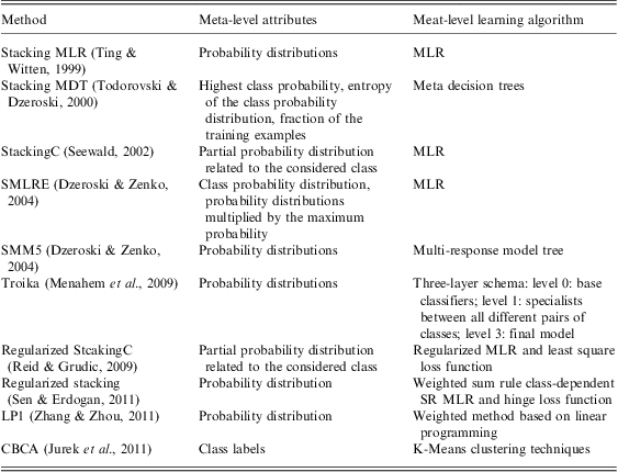
The approach to combining multiple classifiers, based on meta-learning, seems to be very attractive, however, it is less widely used than some other methods. The reason for this may be associated with its complexity and difficulty in theoretical analysis. Compared with standard combining functions introduced in Section 4, the stacking technique is more complicated. Instead of combining the outputs of base classifiers, stacking uses them to build a meta-classifier. It has, however, been proved that this technique can obtain better results compared with other approaches (Dzeroski & Zenko, Reference Dzeroski and Zenko2004). Besides high accuracy, it is worth noting that this technique does not require any specific type of base classifiers. Bagging or boosting, for example, require considerable numbers of models, since they are based on varying data distributions to obtain collections of diverse classifiers by a single learning method. In some cases several dozen base classifiers were used (Bryll et al., Reference Bryll, Gutierrez-Osuna and Quek2003; Machova & Barcak, Reference Machova and Barcak2006; Rodríguez & Maudes, Reference Rodríguez and Maudes2008), which makes the ensemble very large. All of these approaches have to be used for each testing pattern, which is very time-consuming. Stacking may work with only two or three base classifiers and it is not necessary to be concerned if they are stable or not. The two most important issues one should focus on, during the design of the stacking architecture are: the type of attributes that are used for generating level-1 data and the type of level-1 combining method. Table 4 summarizes all of the aforementioned stacking methods.
Summary of the ensemble methods based on meta-learning approach
MDT = meta decision trees; MLR = multi-response linear regression.
5 Ensemble selection
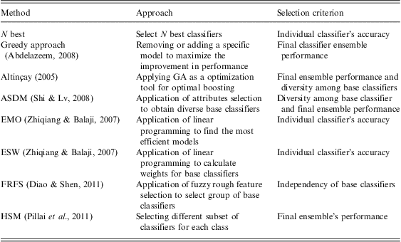
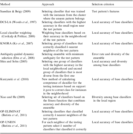
A further approach to combining decisions of base classifiers is based on the selection of the most optimal subset of classifiers. This infers that not all of the generated models contribute during the final decision-making process; however, only a selected group that can obtain the best performance possible are used. This may be considered as a binary weighting process, where the weight is 1 if the classifier is to be considered and 0 otherwise. Ensemble selection can improve the final performance in terms of both accuracy and efficiency (Tsoumakas et al., Reference Tsoumakas, Partalas and Vlahavas2008). The approach allows optimizing the computational cost by reducing the number of base classifiers. In addition to this, it has been shown that a pruned ensemble can obtain improved results in comparison with the original one (Marigineantu & Dietterich, Reference Marigineantu and Dietterich1997). Selection techniques are divided into two categories: static selection and dynamic selection. In the former, a nominated subset of models is selected just once at the beginning and it is fixed for all testing samples. Dynamic selection is performed for each new instance individually, based on its features. In both static and dynamic selections, the key issue is the selection criterion. The most popular criteria in both categories are: diversity measures and individual and combined performance. This may be viewed as intuitive choices, however, correlation between ensemble performance and diversity (Ruta & Gabrys, Reference Ruta and Gabrys2005) and individual accuracy has been questioned (Rogova, Reference Rogova1994).
5.1 Static selection
One of the most simple selection techniques is the Single Best approach, which is based on selecting the best performing classifier over a validation set. The extended version of the approach is referred to as N Best, where models that obtain the N best results are selected. Both of the methods are simple from a computational perspective. Another group of searching algorithms is referred to as the greedy approach (Abdelazeem, Reference Abdelazeem2008). This approach is based on removing or adding a specific model to maximize the improvement in performance. For example, the Forward Search method starts with the best classifier. In each subsequent iteration, a pair of models that reduce the MV error (MVE) are selected and added to the ensemble. The algorithm stops if the MVE cannot be reduced further. A symmetric method to this approach is referred to as Backward search.
A more complicated and popular approach often applied in selecting problem tools, is GAs (Kuncheva & Jain, Reference Kuncheva and Jain2000). A GA may be employed for selecting subsets of base classifiers (Kittler & Roli, Reference Kittler and Roli2001), selecting the single best model (Kittler & Roli, Reference Kittler and Roli2001) or for computing the best fitting base classifier weights (Lam & Suen, Reference Lam and Suen1995). In the study by Altinçay (Reference Altınçay2004), a GA was applied as an optimizing tool for optimal boosting. In the work the classifier prototype along with its training set were evaluated in order to maximize the combined accuracy and ensemble diversity. The proposed technique improved performance of AdaBoost with WMV as a combination function. It was found that by using more than one type of base classifier the accuracy of the proposed method was increased. It was believed that the reason for this was related to increased ensemble diversity.
Four different measures, for selecting the best subset of classifier, were investigated by Löfström et al. (Reference Löfström, Johansson and Boström2008). Two diversity measures: difficulty (DI), double-fault (DF) together with base classifier accuracy (BA) and ensemble accuracy (EA) were tested as a multi-criterion for searching for the best ensemble. First, three groups of ANNs (15 networks each) were trained. A GA was employed as an optimization tool for selecting optimal subsets. MV was used as a combination function. Experiments were carried out with 25 data sets and ANNs as base classifiers. The results demonstrated that applying the two accuracy measures as a multi-criterion was the most efficient approach. Applying the two diversity measures only or a combination of two diversity measures with one of the accuracy measures was found not to be a successful approach.
Different approaches to applying diversity for selecting the best ensemble were introduced by Shi and Lv (Reference Shi and Lv2008). Diversity measures introduced by Melville and Mooney (Reference Melville and Mooney2003) were used, which were directly related with classification results. To obtain the pool of different base classifiers, attribute selection was applied. The proposed algorithm (ASDM-attribute selection and diversity measure) selected random subsets of the original attribute set. The Naive Bayes algorithm was used to obtain one base classifier with each of the subsets. Learned classifiers were added into the ensemble only if the diversity between the classifier and the ensemble was significant. All models from the ensemble were combined using MV. The proposed method outperformed the best single classifier on all attribute subsets. This confirms that, the stable NB classifier can be improved by ensembles based on partitioning of the attributes, as previously demonstrated (Li & Hao, Reference Li and Hao2009).
An alternative approach to selecting models, based on a Data Envelopment Analysis (DEA), was proposed by Zhiqiang and Balaji (Reference Zhiqiang and Balaji2007). The DEA approach was based on LP. It formed an efficient border over the data and computed each data point's effectiveness with reference to this border. Two different methods were investigated. First Efficient Models Only (EMO), which used the DEA formulation to select only the efficient models and then combined them with MV. The second method, namely Efficiency Score Weighting (ESW), was based on weighting each of the base classifiers according to its efficiency score. As a comparison, un-weighted average (UWA) and variance-based weighting (VBW) were applied to the same problems. ESW was found to be the best combining method. The second best approach was EMO, followed by UWA and VBW. In the work of Zhu (Reference Zhu2010), we could observe, however, that ESW and EMO could be outperformed by ensembles constructed by integrating DEA with stacking. All processes were similar to EMO, however, the UWA stacking technique was applied for combining the efficient classifiers. The proposed techniques provided significantly better results than all methods investigated by Zhiqiang and Balaji (Reference Zhiqiang and Balaji2007). In addition, it was compared with bagging, AdaBoost, Random Forest and consequently outperformed them all. It was speculated that the reason for this was related with the application of stacking, which could be deemed as a very effective combining method.
Based on the methods introduced, we can say, that the key issue during static selection of base classifiers is the choice of selection criteria. In the work of Ruta and Gabrys (Reference Ruta and Gabrys2005), a number of selection criteria were introduced and compared. MV was applied as a combining function. They investigated a variety of diversity measures such as correlation coefficient, product–moment correlation, Q-statistics, disagreement measure, double-fault, entropy, measure of difficulty in addition to a few others. Besides this, minimum individual error, mean error, MVE and MV improvement were also considered. All the criteria were applied to different searching algorithms: Random Search, Forward and Backward search, Genetic search and a few others. Based on the results MVE appeared to be the best selection criterion. All searching methods obtained the smallest error, when using MVE as a criterion.
A new static classifier selection method (FRFS) based on rough feature selection was proposed by Diao and Shen (Reference Diao and Shen2011). In this approach, all instances from the training data set were classified by all base classifiers. Following this, the classifier outputs were considered as new attributes. In other words, each base classifier represented one attribute that can have any class label as a value. In the next step, fuzzy rough feature selection (Jensen & Shen, Reference Jensen and Shen2009) was performed on the new data set. Harmony Search (Geem et al., Reference Geem, Kim and Loganthan2001) was subsequently applied to optimize the quality of the subsets of the features by reducing its size. Selected in this way, the subset of features indicated the corresponding classifiers that could be included in the classifier ensemble. FRFS was compared with the individual classifiers and the full ensemble, where all base classifiers contribute to the final decision. The reduced ensemble did not outperform the full collection of classifiers in most of the data sets, it was, however, very comparable. In most of the cases, it provided a good improvement over the accuracy of the base classifiers.
Classifier selection for multi-label problems was presented by Pillai et al. (Reference Pillai, Fumera and Roli2011). The idea of this work was to select possible different subsets of classifiers for each class. In other words, for each class, the decision if instance x belongs to this class or not should be made by combining outputs coming from different subsets of classifiers. This approach was referred to as the hybrid selection of multi-label classifiers (HSM). For selecting classifiers two static criteria were developed based on the micro and macro averaged F-measure. The proposed HSM was compared with the standard selection method where the same subset of classifiers is selected for each class and the full ensemble. Experimental results indicated that the new approach outperformed the other two methods.
5.2 Dynamic selection
The methods introduced in the previous section have been based on the static selection of the subset of base classifiers. A range of work, however, has been carried out in relation to dynamic classifier selection. Generally, dynamic selection can be considered in two ways: dynamic classifier selection and dynamic ensemble selection. In the former, for each test pattern, a set of classifiers is nominated to create an ensemble. While in the latter, the most suitable combination is selected from the pool of predefined ensembles. In the work of Saeedian and Beigy (Reference Saeedian and Beigy2009) for each testing instance, only one individual classifier was selected to make a final decision. All data from the training set were clustered using the k-means algorithm. One base classifier was built with each of the clusters applying SVM as a learning method. For new instances, the closest cluster was identified. The model built with this cluster was nominated to make a final decision. The proposed method outperformed MV in a spam filtering problem.
One of the most popular techniques of dynamic selection is Dynamic Classifier Selection by Local Accuracy (DCS-LA) (Woods et al., Reference Woods, Kegelmery and Bowyer1997). This approach was based on estimating all of the base classifiers’ local accuracy in the small region of the feature space, in the neighborhood of the test pattern. The most locally accurate classifiers were employed to make a final decision. It has been shown (Cevikalp & Polikar, Reference Cevikalp and Polikar2008), however, that DCS-LA can be outperformed by the related method referred to as Local Classifier Weighting by Quadratic Programming. In this approach, for a given query, non-negative weights were determined for classifiers in the ensemble. Weighting was based on their accuracy in the neighborhood of the given test pattern. More effective models were weighted more heavily for making final decisions. AdaBoost with ANNs as a learning method was used to train base classifiers. The proposed method outperformed DCS-LA in most of the cases considered. Both schemes, however, outperformed in all cases the other combining methods considered during the experiments such as MV, WMV, Max, Sum and Product Rules.
Other dynamic classifier selection methods related to DCS-LA were Local Class Accuracy (Woods et al., Reference Woods, Kegelmery and Bowyer1997), a priori and a posterior (Didaci et al., Reference Didaci, Giacinto, Roli and Marcialis2005) and K-nearest-oracles (KNORA; Ko et al., Reference Ko, Sabourin and Britto2007). All of them aimed to find classifiers that will be the most likely to be correct for a pattern in a pre-defined neighborhood. KNORA differed from the others, given that instead of selecting the most suitable model, it looked for the most suitable ensemble. For a test pattern, its K-NNs from the validation set were selected. A group of classifiers that correctly classify those neighbors were selected and applied as an ensemble to provide a final decision. All of the aforementioned methods and four extended versions of KNORA were introduced and compared by Ko et al. (Reference Ko, Sabourin and Britto2008). Additionally, they were compared with static methods such as GA with MVE that was considered as one of the best selecting classifier criteria (Ruta & Gabrys, Reference Ruta and Gabrys2005). Experiments on handwritten numerals demonstrated that the proposed scheme (KNORA-ELIMINATE) with MV as the combining function was the best of the dynamic techniques, and slightly outperformed the static method. Nevertheless, methods like OLA and a priori, were not as effective as GA with MVE.
A number of dynamic methods rather than selecting from a group of base classifiers select from a group of previously generated ensembles. A method based on this approach, referred to as Ambiguity-Guided Dynamic Selection, was proposed by Dos et al. (Reference Dos Santos, Sabourin and Maupin2008). The process of this method first involved applying a random subspace selection to generate a pool of base (C4.5) classifiers. Second, to obtain a collection of ensembles, an optimization process was carried out (GA) with error rate and diversity as the criteria. The next step was selecting an ensemble with the minimum ambiguity for the given testing patterns. The minimum ambiguity value leads to the maximal margin that leads to an increase in the certainty of classification. The margin was considered as a difference between the support provided to the selected class and the support provided to all the other classes. MV was used for combining classifiers in the ensemble. The proposed method was compared with DCS-LA and static ensemble selection using a generated population. Experiments were carried out on three different data sets. The ambiguity-guided method outperformed DCS-LA, however, the static method provided the best results in most of the cases.
Different dynamic selection methods, based on accuracy and error diversity, were introduced by Shin and Sohn (Reference Shin and Sohn2005). First, a collection of decision trees was designed on the basis of bootstrap samples. All individual models were clustered using Shannon and Banks (Shannon & Banks, Reference Shannon and Banks1999) distance metric with an appropriate number of clusters. For new testing instances, its K-nearest neighbors were identified. Two clusters were selected: first with the highest classification accuracy in the local region and second with the longest mean distance from the first one. Classifiers from both clusters were combined using MV. The method was compared with DCS-LA, boosting, bagging and single C4.5. The results demonstrated that the proposed technique outperformed all the rest when the number of base classifiers was relatively big (50, 75, 100). Bagging seemed to be most effective for a small number of bootstrap samples (10, 25).
Kurzynski et al. (Reference Kurzynski, Woloszynski and Lysiak2010) proposed new methods for calculating the competence of a classifier for a given instance. The potential function model for calculating the competence of a classifier Com(C ∣ x) for classifier C for unseen object x is given in the following equation:
 $$Com(C\,|\,x)\, = \,\mathop{\sum}\limits_{{{x}_k} \in V} {Co{{m}_{src}}\,(C\,|\,{{x}_k})\,\times \,{{e}^{({\rm{ - }}d{{{(x,{{x}_k})}}^{\rm{2}}} )}} } $$
where  $$\[--><$>Co{{m}_{src}}(C|{{x}_k})<$><!--$$
is the source competence of classifier C for instance xk from validation set V and d(x, xk) is the Euclidean distance between x and instance xk. In this study, a new successful method of calculating source competence was proposed as expressed in the following equation:
 $${{C}_{scr}}(C\,|\,{{x}_k})\, = \,{\rm{2}}\,\times \,{{C}_{jk}}\,{{({{x}_k})}^{\tfrac{{\log ({\rm{2}})}}{{\log (m)}}}} {\rm{ - 1}}$$
where Cjk(xk) is the support given by the classifiers for the correct class of xk. It can be noted that the function has values in the closed interval [−1, 1]. It can also be noted that the value is equal to 1 if maximum support is given to the correct class and −1 support given to the correct class if the value is equal to 0. For unseen instances all classifiers with a competence >0 were selected for the final ensemble. The proposed technique outperformed four other methods based on similar approaches namely DCS-LA (Woods et al., Reference Woods, Kegelmery and Bowyer1997), DCS-MBC (Giacinto & Roli, Reference Giacinto and Roli2001), DSC-MLA (Smits, Reference Smits2002) and DES-KE (Ko et al., Reference Ko, Sabourin and Britto2008). It also obtained better average accuracy than a single classifier and the MV method.
In the study of Xiao and He (Reference Xiao and He2009), a new external criterion of selecting a classifier ensemble based on accuracy and diversity in the local region was proposed. For each test pattern, they aimed to select the optimal complexity model according to the following equation:
 $$Fitness\, = \,{{d}^{\rm{2}}} (W)\, + \,\lambda \,\times \,D{{F}_{av}}$$
where  $$\[--><$>{{d}^{\rm{2}}} (W)\, = \,{{\rDelta }^{\rm{2}}} (A){\rm{ - }}{{\rDelta }^{\rm{2}}} (B)<$><!--$$
and
 $$\[--><$>{{\rDelta }^{\rm{2}}} (A)<$><!--$$
represents classification error on the set B by the model trained with set A and
 $$\[--><$>{{\rDelta }^{\rm{2}}} (B)<$><!--$$
represents the classification error on set A by the model trained on set B. DFav is the average value of double-fault diversity measure between every two classifiers in the ensemble. Parameter λ determines the influence of diversity. The results indicated that the proposed method (GDES-AD) has a strong noise resistance compared with some other methods based on similar approaches like C-V, DCS-LA and KN-U. GDES-AD significantly outperformed all other methods when the data set contains some noise. For data sets without artificial noise it performed lower than some other techniques.
Two new strategies for dynamic selection, namely OP-ELIMINAT and OP-UNION, were presented by Batista et al. (Reference Batista, Granger and Sabourin2011). Both methods were based on K-nearest oracles. The first step, in both cases, was for a new instance to select its k number of nearest neighbors. For OP-ELIMINATE, all base classifiers were tested on the selected subset and only those that classified all k neighbors correctly were included into the ensemble. If there were no classifiers, then the parameter k was decreased. For OP-UNION the selection process was different. For each selected neighbor, they searched for k base models that classified the instance correctly. All selected classifiers form the final ensemble. The new methods outperformed two previously described methods KNORA-UNION/ELIMINATE (Ko et al., Reference Ko, Sabourin and Britto2008) and MV combination of 100 SVM classifiers. Based on the evaluation conducted, OP-ELIMINATE obtained the lowest overall error rates.
Tables 5 and 6 summarize all static and dynamic methods described in this paper. We can notice that with the static approach to selecting base classifiers, the most common selection criteria are accuracy and diversity among base classifiers. For the dynamic methods, however, the most frequently used selection criterion is based on the local accuracy of the models.
Summary of static methods for base classifier selection
ASDM = attribute selection and diversity measure; EMO = Efficient Models Only; ESW = Efficiency Score Weighting; HSM = hybrid selection of multi-label classifiers.
Summary of dynamic methods for base classifier selection
Both static and dynamic base classifier selections seem to be effective methods of improving classifier ensemble accuracy. In the static method, the optimal solution is obtained from training data, where the class labels are known, however, it does not have to be optimum for unseen data. Dynamic methods deal with this problem by taking into account the test pattern's features during selecting the classifiers, for example, with the KNORA approach (Ko et al., Reference Ko, Sabourin and Britto2007). To overcome this problem, in static methods, the true accuracy of the ensemble should be estimated based on the data that have not been applied for selecting the optimum classifier or for building individual classifiers. This, however, requires a larger training set. On the other hand, static techniques should be more efficient with respect to execution time. If the number of base classifiers is large, it can moderate the search algorithm. Given that in dynamic selection, the optimization process is performed for each instance individually, it can dramatically extend the testing time.
All of the methods described above can be applied with both a group of base classifiers: generated using the same learning algorithm and different training set (bagging, boosting) or different learning methods and the same training data. It is difficult to agree which approach is more effective, since limited comparisons between them have been presented to date. The selection of base classifiers seems to be very efficient in the combining process. It is useful especially in the situations when a large number of base classifiers are generated (like in the instances of bagging or boosting techniques). It not only increases accuracy, however, it also reduces the complexity of the ensemble.
6 Summary
The problem of combining multiple classifiers has been investigated by a number of studies in recent years. There are many different approaches to this problem and many different techniques have already been proposed. It is very difficult to compare all of the techniques and subsequently decide which of them is the most effective. In this paper, we aimed to provide an overview of the most significant work that has been conducted with regard to the ensemble methods. We hope that it has provided a deeper insight into the techniques, challenges and trends within these areas and can help others to understand the ensemble process with the aim of stimulating new ideas and new directions in the area of generating classifier ensembles.
We have mainly focused on the three most well-known techniques: bagging, boosting and stacking and provided a review of the different improvements of these three techniques that have been proposed by a range of different studies. Each of the techniques has some features that make them more or less suitable for different learning methods. Bagging and boosting are both based on the same general concept of generating a diverse classifier ensemble by manipulating the training data set, which is subsequently given to a base learning algorithm. According to the methods considered, boosting seems to perform better and does not require such a high level of instability of learning method compared with bagging. Bagging, however, manages better with classification noise in data and it can obtain improved results in instances when a smaller number of training data is available, compared with boosting. Stacking was compared with bagging and boosting in a number of studies and it was considered as the leading technique. In addition to this, stacking does not require any special type and number of base classifiers. This is a significant advantage compared with the two other methods, where a large number of models are required.
In addition, we provided a review of existing classifier ensemble selection methods based on both static and dynamic approaches. The main research question within this study has aimed to answer what is the best choice of the selection criterion. To help to understand why and how the ensembles work, we reviewed a number of existing theoretical studies regarding the classifier ensemble problem. Some conclusions can be drawn via reviewing the most recent studies:
• The main focus with the bagging technique is related to increasing diversity among base classifiers. In recent studies, there were some successful solutions proposed based on applying some selection criteria rather than applying all base classifiers (Datta & Pihur, Reference Datta and Pihur2010; Zeng et al., Reference Zeng, Chao and Wong2010) or performing a clustering process instead of random sampling to obtain different training sets (Gan & Xiao, Reference Gan and Xiao2009).
• Most of the recent study regarding boosting techniques focused on adapting it to stable classifiers, with the main focus on k-NN classifier. A successful solution can be considered as a modification of the input space of k-NN (García-Pedrajas & Ortiz-Boyer, Reference García-Pedrajas and Ortiz-Boyer2009; He et al., Reference He, Song, Shen and Hai2010) or applying different values of parameter k depending on level of difficulty of the unseen pattern (Murrugarra-Llerena & Lopes, Reference Murrugarra-Llerena and Lopes2011).
• An alternative to the bagging or boosting method of generating an ensemble can be the training of each base classifier in different feature subspaces (Li & Hao, Reference Li and Hao2009; Tahir & Smith, Reference Tahir and Smith2010).
• Application of regularization to linear stuck generalization remedies the over-fitting problem and improves its overall performance (Reid & Grudic, Reference Reid and Grudic2009; Sen & Erdogan, Reference Sen and Erdogan2011).
• While combining decisions of base classifiers, it is effective to differentiate the reliability of the predictions of each base classifier among classes (Parvin & Alizadeh, Reference Parvin and Alizadeh2011). In the previous study, contribution of the base classifiers to the final decision was based on its accuracy similar to the case of weighted MV.
• A semi-supervised learning method can be successfully applied as a meta-level learning method in stacking techniques. It enables stacking to be applied with only a partially labeled validation set (Jurek et al., Reference Jurek, Bi, Wu and Nugent2011).
It could be noticed that only in one of the aforementioned approaches (Jurek et al., Reference Jurek, Bi, Wu and Nugent2011), a clustering technique was considered for the purpose of generating classifier ensemble. It has been presented that an ensemble based on such an approach can provide good results in terms of classification accuracy. Besides this, the advantage of performing classification by clustering analysis is that once the final model is trained, it is computationally efficient and no base classifiers are required while assigning a class label to a new instance. Development of a new classifier ensemble methods based on clustering analysis can be considered as new research direction in ensemble learning. Application of unsupervised learning methods permits consideration to be directed towards unlabeled data in the training set what can be appreciated in real-world applications where collecting labeled data may be a costly process. Application of unlabeled data in ensemble learning is a quite new research direction, which has received limited attention to date. It has been presented, however, that unlabeled data can be very beneficial for ensemble learning (Zhou, 2009).