Non-separability and substitutability among water pollutants: evidence from India

Surender Kumar; Shunsuke Managi

doi:10.1017/S1355770X11000283

Non-separability and substitutability among water pollutants: evidence from India

Published online by Cambridge University Press: 31 August 2011

Surender Kumar and

Shunsuke Managi

Show author details

Surender Kumar: Affiliation:
Department of Business Economics, University of Delhi, India. Email: surenderkumarbansal@hotmail.com
Shunsuke Managi: Affiliation:
Graduate School of Environmental Studies, Tohoku University, 6-6-20 Aramaki-Aza Aoba, Aoba-Ku, Sendai 980-8579, Japan; and Institute for Global Environmental Strategies, Japan. Tel: 81-45-339-3751. Fax: 81-22-795-4309. Email: managi.s@gmail.com

Article contents

Abstract
Introduction
Background
Theoretical and empirical framework
Data and results
Discussion and conclusions
Footnotes
References

Rights & Permissions

Abstract

The design and implementation of environmental policy often involve more than one pollutant, and must consider pollution as a byproduct of the production of marketable output. In this paper, we test the implicit assumption in the empirical literature that (1) production of marketable output, pollution and abatement are separable, and (2) different pollutants can be abated separately. Using unique plant-level data in India, we reject the null hypotheses of separability between marketable output and pollutants, and between different pollutants. Firms must incur abatement costs for reducing pollution levels. In addition, complement and substitute relationships between water pollutants are demonstrated with statistical significance.

Information

Type: Research Article
Information: Environment and Development Economics , Volume 16 , Issue 6 , December 2011 , pp. 709 - 733

DOI: https://doi.org/10.1017/S1355770X11000283 [Opens in a new window]
Copyright: Copyright © Cambridge University Press 2011

1. Introduction

In the conventional empirical environmental economics literature, there are usually two implicit assumptions. The first assumption is that the production of marketable output, pollution and abatement are separable. For example, Smith (Reference Smith1998) notes that a common production index assumes marketable outputs are separable from the pollution. This assumption precludes the options of controlling pollution through changes in production processes and input substitutions, and relies only on end-of-pipe treatment technology. This is because the production side is excluded in abatement evaluation. However, less pollution can be made possible by changes in production processes and reassignment of capital (i.e., input substitutions) (Yohe, Reference Yohe1976; Anderson, Reference Anderson1987). Computationally, Kuper and Van Soest (Reference Kuper and Van Soest2003) show production processes and input substitutions play a crucial role in the results. Clean technology plays an important role in pollution management, and sound environmental policy must consider pollution as a byproduct of the production of marketable output (Montero, Reference Montero2001). Given the importance of such restrictions to the interpretation of environmental policy, further discussion of the assumption would help to understand this approach.

The second assumption is that different pollutants are abated separately. Previous studies often focus on the regulation of a single pollutant.Footnote ¹ Many production processes are, however, accompanied by multiple emissions of pollutants. This assumption precludes abatement technologies that allow for the joint abatement of several pollutants. Recent abatement technologies, however, allow for the joint abatement of several pollutants and the choice of input mix needs to be treated concurrently. Therefore, in general, abatement decisions cannot be made separately for each pollutant level (Eskeland, Reference Eskeland1997).

For example, biological oxygen demand (BOD) and chemical oxygen demand (COD) are measures of organic water pollution, and reduction in one pollutant often entails reduction in another, implying that these pollutants complement one another in the abatement process. Another example shows that pollutants may also substitute for one another. The abatement of sulfur dioxide (SO₂) emissions from power plants requires considerable energy, leading to an increase in carbon dioxide (CO₂) emissions. These general assumptions are very rarely tested in empirical applications, which leads to potential biases in policy recommendations. For example, if two pollutants are complements, we overestimate the true abatement compliance cost for each pollutant. If pollutants are substitutes, we underestimate the cost. Also, there might be an unintended consequence of increases in one pollutant by reductions in another pollutant. The aim of this study is to empirically test such assumptions.

In one recent study, Moslener and Requate (Reference Moslener and Requate2007) find that, using a framework where the abatement costs of several pollutants are non-separable, optimal emission paths are qualitatively different for substitutes and complements, even if the pollutants are symmetric with respect to both their abatement costs and the damage they cause. The authors obtain non-monotonic behavior in the emission abatement paths.Footnote ² They call for empirical research that estimates substitutability/complementarity between different pollutants using non-separable functions of marketable output, pollution and abatement. Results of these empirical studies will be useful for setting policy tables of optimal pollution reduction targets, and thereby developing appropriate policy instruments.

Abatement cost has been analyzed in the framework of production efficiency (see Färe et al., Reference Färe, Grosskopf, Noh and Weber2005; Huhtala and Marklund, Reference Huhtala and Marklund2008). Huhtala and Marklund (Reference Huhtala and Marklund2008) show the connection between the environmental preferences of society and the opportunity costs of firms at the social optimum constrained by environmental regulations. Using a directional distance function approach, they provide a theoretical justification for our model to analyze associations between productive/environmental efficiency and marginal abatement cost. The questions of separability and substitutability can be addressed well in this framework. Weaver (Reference Weaver1998), Coelli et al. (Reference Coelli, Lauwers and Van Huylenbroeck2007) and Welch and Barnum (Reference Welch and Barnum2009) analyze separability and substitutability associated with abatement costs and efficiency. Furthermore, the substitution relationship within energy sources of electricity generation in the US is discussed by Welch and Barnum (Reference Welch and Barnum2009). They consider externalities associated with the disposal of residuals resulting from the consumption and production process in their general equilibrium model. Instead of their complex mathematical modeling for substitutions and other relationships, our study intends to identify its relationship in a computationally simple way.

In this study, we adopt a joint production technology approach followed by Färe et al. (Reference Färe, Grosskopf, Noh and Weber2005), Murty et al. (Reference Murty, Kumar and Dhavala2007) and Huhtala and Marklund (Reference Huhtala and Marklund2008). We apply this model to Indian water-polluting industries. Applications in developing countries are important because water pollution is currently the key pollution problem in these countries, and regulations are regularly implemented because of this problem.

We use a directional output distance function for testing the separability of marketable output and pollutants, as well as the interaction between pollutants within given sets of pollutants. The directional distance function simultaneously seeks to expand marketable output and to contract pollutants. Moreover, the function treats marketable output and pollutants asymmetrically. That is, outputs can be either strongly or weakly disposable. Strong disposability implies that a firm can reduce pollutants without incurring any abatement costs. Weak disposability assumes diversion of resources from the production of marketable output.

The function is specified parametrically with a quadratic functional form, and is used to estimate the combined environmental and technical efficiency, shadow prices of BOD, COD and suspended solids (SS), and the elasticity of substitution between marketable output and pollutants, as well as within pollutants. Though BOD and COD are expected to be complements (because of the similarity in their measurement targets), SS may not be a complement to BOD and COD. The directional output distance function could be estimated either deterministically or stochastically (e.g., Kumar and Managi, Reference Kumar and Managi2009; Fujii et al., Reference Fujii, Kaneko and Managi2010). The deterministic procedure accounts for all deviations from the observed frontier in measuring inefficiency. Some of the deviations of observed outputs from the frontier, however, might be due to measurement and random errors. Therefore, the directional output distance function is estimated as a stochastic frontier in this paper. We find that the production of marketable output cannot be separated from the production of pollutants, and that the production (or, for that matter, abatement) of one pollutant cannot be separated from the production of another pollutant. We also find complementarity in the abatement of BOD and COD effluents, though there is substitutability in the abatement of BOD (and COD) effluent and the effluents of SS.

The remainder of the paper is organized as follows. The literature review is provided in section 2. Section 3 specifies the theoretical and empirical framework of the joint production of marketable output and pollutants. Section 4 discusses the data and empirical results, and section 5 summarizes the study and provides some concluding remarks.

2. Background

Separability and substitutability in the context of abatement costs and efficiency are discussed in Weaver (Reference Weaver1998), Coelli et al. (Reference Coelli, Lauwers and Van Huylenbroeck2007) and Welch and Barnum (Reference Welch and Barnum2009). For a recent study, Welch and Barnum (Reference Welch and Barnum2009) consider the substitution relationship within energy sources of electricity generation in the US. The separability assumption has been considered in the theoretical and empirical literature, though there are few formal empirical tests.Footnote ³ Schwabe (Reference Schwabe1999) shows that relaxing separability assumptions can increase efficiency gains for marketable permits to command and control. Similarly, Wossink et al. (Reference Wossink, Lansink and Struik2001) illustrate that the production of marketable output, pollution and abatement are decided simultaneously and cannot be treated separately.

In the empirical literature, two approaches relate to separability assumptions. One assumes that marketable output is separable from the production of pollutants (or pollution abatement). For example, Bellas (Reference Bellas1998), Goldar et al. (Reference Goldar, Misra and Mukherji2001) and Dasgupta et al. (Reference Dasgupta, Huq, Wheeler and Zhang2001) estimate marginal abatement costs assuming separability between marketable output and pollutants. The second method considers non-separability and models joint production of marketable output and pollution. Kolstad and Turnovsky (Reference Kolstad and Turnovsky1998), Carlson et al. (Reference Carlson, Burtraw, Cropper and Palmer2000), Domazlicky and Weber (Reference Domazlicky and Weber2004), Managi et al. (Reference Managi, Opaluch, Jin and Grigalunas2005), Murty et al. (Reference Murty, Kumar and Dhavala2007) and Kumar and Managi (Reference Kumar and Managi2010) consider pollution a byproduct of the production of marketable output. The second method has the advantage of analyzing the abatement effort in terms of reduced production of the marketable output that results from reducing a pollutant, and captures synergies in the joint abatement of multiple pollutants.

The design and implementation of good environmental policy necessarily involve more than one pollutant (Eskeland, Reference Eskeland1997). Beavis and Walker (Reference Beavis and Walker1979) show that the standard and tax approachesFootnote ⁴ for controlling environmental pollution (based on the assumption of separability in joint abatement cost functions) lead to sub-optimal environmental policy when there are multiple pollutants that are simultaneously generated and abated.

Montero (Reference Montero2001) and Schmieman et al. (Reference Schmieman, van Ierland and Hordijk2002) recognize the importance of interactions between pollutants for policy, and theoretically model the joint abatement of various pollutants. Greenstone (Reference Greenstone2003) empirically examines the effect of reducing air pollution in the iron and steel industry between 1987 and 1997, and finds that the lead, particulate matter and ground level ozone non-attainment designations of the Clean Air Act Amendments are associated with reductions in total emissions of these pollutants. Thus, he finds little evidence of substitutes among pollutants. Burtraw et al. (Reference Burtraw, Krupnick, Palmer, Paul, Toman and Bloyd2003) calculate the reduction in SO₂ and nitrogen oxides emissions as an ancillary effect of reducing CO₂ emissions. Dellink (Reference Dellink2005), using computational general equilibrium modeling, estimates the abatement costs for different pollutants and analyzes the interaction between different environmental themes, such as climate change and smog formation (and their implications for regulation). Considine and Larson (Reference Considine and Larson2006) treat emissions as an input (instead of an undesirable output) in electric utilities and estimate Morishima elasticity of substitution. They find that emissions and high sulfur coal are complements, and that emissions and low sulfur coal are substitutes. None of the studies, however, tests the two assumptions empirically in terms of economic production. In addition, analysis undertaken for India is unique because of its economic and environmental significance.

3. Theoretical and empirical framework

3.1. The directional output distance function and non-separability among outputs

To test for non-separability of marketable output and simultaneously produced pollutants in the production process, and within various pollutants, we use a directional output distance function. This function also measures substitutability among different pollutants. A directional output distance function seeks to expand the vector of marketable outputs, y ∈ ℛ₊^M, and reduce the vector of pollutants (such as BOD, COD and SS effluents), b ∈ ℛ₊^N, by employing a vector of inputs (such as labor, capital and materials), x ∈ ℛ₊^l. The function inherits its properties from the production technology, P(x). The production technology is defined as:

(1)

$P\lpar x\rpar = \lcub \lpar x\comma \; y\comma \; b\rpar \, \colon \, x \, \hbox{can produce}\lpar y\comma \; b\rpar \rcub . \eqno\lpar 1\rpar$

The production technology may be modeled in alternative ways. The outputs are strongly or freely disposable if (y, b) ∈ P(x) and (y′, b′) ≤ (y, b) ⇒ (y′, b′) ∈ P(x). This implies that if an observed output vector is feasible, then any output vector smaller than that is also feasible. This assumption excludes production processes which generate pollutants that are costly to dispose of. Concerns for pollution reduction require that these should not be considered freely disposable. In such cases, bad outputs are considered weakly disposable: (y, b) ∈ P(x) and 0 ≤ θ≤ 1 ⇒ (θ y, θ b) ∈ P(x). This implies that pollution disposal is costly and that abatement activities would typically divert resources away from the production of marketable outputs, leading to lower marketable outputs for given inputs or the employment of more resources for a given level of marketable output. Marketable outputs are assumed to be null-joint with the pollutants.Footnote ⁵ Formally, the directional output distance function is defined as:

(2)

$D\lpar x\comma \; y\comma \; b\semicolon \; g\rpar = \mathop {\max}\limits_\beta \lcub \beta \colon \lpar y + \beta \cdot g_y\comma \; b - \beta \cdot g_b \rpar \in P\lpar x\rpar \rcub . \eqno\lpar 2\rpar$

This function requires a simultaneous reduction of pollutants and expansion of marketable outputs. The computed value of β (i.e., β*) provides the maximum expansion of marketable outputs and reduction of pollutants if a firm has to operate efficiently given the directional vector g. The vector g = (g _y, −g _b) specifies the direction in which an output vector ((y, b) ∈ P(x)) is scaled, so as to reach the boundary of the output set at the point (y = β* · g _y, b − β * · g _b) ∈ P(x). This is accomplished by expanding marketable outputs and reducing pollutants, where β* = D(x, y, b; g).

The directional output distance function derives its properties from the output possibility set, P(x) (see Färe et al., Reference Färe, Grosskopf, Noh and Weber2005).Footnote ⁶ These properties include monotonicity conditions for marketable outputs and pollutants and, from its definition, a translation property that is the additive counterpart to the homogeneity property of the Shephard distance functions. The translation property implies that:

(3)

$D \lpar x\comma \; y + \alpha\comma \; b - \alpha\semicolon \; g_y\comma \; - g_b \rpar + \alpha = D\lpar x\comma \; y\comma \; b\semicolon \; g_y\comma \; - g_b\rpar . \eqno\lpar 3\rpar$

Moreover, the advantage of a directional output distance function is that it allows one to consider disproportional changes in outputs, and makes it possible to expand one output while reducing another. The distance function takes the value of zero for technically efficient output vectors on the frontier, whereas positive values imply inefficient output vectors below the frontier. The higher the value, the more inefficient is the output vector.

The directional output distance function is parameterized using a (additive) quadratic flexible functional form, following Färe et al. (Reference Färe, Grosskopf, Noh and Weber2005). In our case, the particular form is expressed as follows, with one marketable output (y ₁), three pollutants (BOD = b ₂, COD = b ₃ and SS = b ₄), and three inputs (materials = x ₁, wages = x ₂ and capital stock = x ₃):

(4)

$\eqalign{D\lpar x\comma \; yb\semicolon \; g\rpar &= \alpha_0+\sum\limits_{l = 1}^3 \, \beta _l x_l + \alpha_1 y_1 + \sum\limits_{n = 2}^4 \, \alpha _n b_n + {1 \over 2}\sum\limits_{l + 1}^3 \, \sum\limits_{l^{\prime} = 1}^3 \, \alpha _{ll^{\prime}} x_l x_{l^{\prime}} \cr & \quad + \sum\limits_{l = 1}^3 \, \gamma _{l1} x_l y_1 + \sum\limits_{n = 2}^4 \, \sum\limits_{l = 1}^3 \, \gamma _{nl} b_n x_l \cr & \quad + {1 \over 2}\alpha_11 y_1^2 + \sum\limits_{n = 2}^4 \, \alpha _{1n} y_1 b_n + {1 \over 2}\sum\limits_{n = 2}^4 \, \sum\limits_{n^{\prime} = 2}^4 \, \alpha _{nn^{\prime}} b_n b_{n^{\prime}} + \phi _t t + \phi _p I} \eqno\lpar 4\rpar$

with

$\eqalign{\beta_{ll^{\prime}} &=\beta _{l^{\prime}l}\semicolon \; \alpha_{nn^{\prime}} = \alpha_{n^{\prime}n}\semicolon \; \alpha_1 - \sum\limits_{n = 2}^4 \, \alpha _n = - 1\semicolon \; \alpha _{1n} - \sum\limits_{n = 2}^4 \, \alpha _{nn^{\prime}} = 0\semicolon \; \alpha_11 \cr & \quad - \sum\limits_{n = 2}^4 \, \alpha _{1n} = 0\semicolon \; \gamma _{l1} - \sum\limits_{n = 2}^4 \, \gamma _{\ln} = 0\semicolon \; l = 1\comma \; 2\comma \; 3\semicolon \; n = 2\comma \; 3\comma \; 4}$

This study includes time and industry dummies in the estimation of the directional distance function. We note that potentially the panel data structure could be employed to distinguish between cross-individual heterogeneity and inefficiency (Greene, Reference Greene, Fried, Lovell and Schmidt1993).

The constraints follow from the translation property, and g = (1, −1), where 1 refers to marketable output and −1 refers to the pollutant direction vector. Furthermore, t are time dummies, and I _p are industry dummies.

Production of marketable output is separable from the production of pollutants or the production of a single pollutant, say BOD, and is separable from the production of another pollutant, say COD, if the following condition is satisfied:

(5)

$\underbrace {{\partial \over \partial y_1}\left({D_i \over D_j} \right)\equiv 0}_{between\; good\; and\; bad\; outputs}\; \comma \; {\rm {and}} \underbrace {{\partial \over\partial b_k}\left({D_i \over D_j} \right)\equiv 0}_{within\; bad\; outputs}\comma \; \lpar i\comma \; j\comma \; k\rpar \in \Re_+^N \eqno\lpar 5\rpar$

In other words, for the outputs to be functionally separable in a quadratic directional output distance function, following Blackorby et al. (Reference Blackorby, Primont and Russell1977), first- and second-order derivatives of the distance function should satisfy the following condition:

(6)

$\underbrace {D_i D_{j1} - D_j D_{i1} = 0}_{between\; good\; and\; bad\; outputs}\comma \; {\rm {and}}\underbrace {D_i D_{jk} - D_j D_{ik} = 0}_{within\; bad\; outputs} \eqno\lpar 6\rpar$

where the subscripts on the distance functions refer to first- and second-order partial derivatives with respect to outputs. For example, D _j is the first-order partial derivative of the distance function with respect to b _j, and D _jk is the second-order derivative of the distance function.

3.2. Marginal abatement costs of pollutants

Färe et al. (Reference Färe, Grosskopf, Lovell and Yaisawarng1993) was the first study estimating the marginal abatement costs (shadow prices) of pollutants using an output distance function that considered non-separability between different outputs. The output distance function projects the observed output vector onto the boundary of the output set by increasing all outputs proportionally, including pollutants. However, in the case of a directional output distance function, it is possible to project to the frontier in a direction that decreases pollutants and increases marketable output. Färe et al. (Reference Färe, Grosskopf, Noh and Weber2005) estimated the marginal abatement cost for SO₂ emissions using a directional output distance function. Following this study, Murty et al. (Reference Murty, Kumar and Dhavala2007) estimated the marginal abatement cost functions for air pollutants in a non-separable production framework. The derivation of marginal abatement costs using a distance function requires the assumption that one observed output price is its shadow price. Let y ₁ denote the marketable output, and assume that the observed marketable output price equals its absolute shadow price (r ₁^o = r ₁^s). Färe et al. (Reference Färe, Grosskopf, Noh and Weber2005) have shown that the marginal abatement cost for pollutant, b _i (i = 2, …, N) can be derived as

(7)

$r_i^s = r_1^o {\partial D/ \partial b_i \over \partial D/ \partial y}\comma \; i = 2\comma \; 3\comma \; \ldots\comma \; N. \eqno\lpar 7\rpar$

3.3. The Morishima elasticity of substitution

A directional output distance function can be used to measure the interaction between different outputs, as it completely describes the production technology, including curvature. The curvature measures the ease with which marketable outputs can be substituted with pollutants, and the ease with which pollutants are substituted for one another in the production process. The curvature can be quantified using the concept of Morishima elasticity of substitution, which is the ratio of relative change in the shadow prices of marketable output and pollution to the relative change in pollution intensity (i.e., the ratio of bad output to good output). Following Blackorby and Russell (Reference Blackorby and Russell1989) and Färe et al. (Reference Färe, Grosskopf, Noh and Weber2005), the indirect Morishima elasticity of substitution between outputs may be defined as:

(8)

$M_{i1} = {d \ln\lpar q_i /p\rpar \over d \ln\lpar y/b_i \rpar }\comma \; {\rm {and}} \; M_{ij} = {d \ln\lpar q_i /q_j \rpar \over d \ln\lpar b_j /b_i \rpar } \eqno\lpar 8\rpar$

where q and p stand for the prices of bad and good outputs respectively; and in terms of directional output distance function, the Morishima elasticity of substitution, following Färe et al. (Reference Färe, Grosskopf, Noh and Weber2005), between marketable output and pollution (and within pollutants) can be specified as:

(9)

$M_{i1} = y^{\ast} \left({D_{i1} \over D_i} - {D_{11} \over D_1} \right)\comma \; {\rm {and}} \; M_{ij} = b_j^{\ast} \left({D_{ij} \over D_i} - {D_{jj} \over D_j} \right)\eqno\lpar 9\rpar$

where y* and b* are the frontier values of marketable output and pollution, respectively. Given the monotonicity and concavity properties of the directional distance function with respect to good and bad outputs, the sign of M _i1 should be negative along the positively sloped portion of P(x) (when the bad outputs are assumed to be weakly disposable). The higher values of M _i1 (in absolute terms) indicate that a given change in the ratio of outputs will yield higher changes in the shadow price ratio. Therefore, as the elasticity of substitution becomes more negative, it becomes more costly to reduce pollution. Moreover, the Morishima elasticities are not symmetric, i.e., M _i1 ≠ _M1i. This is as it should be and allows for asymmetry in the substitutability of different outputs.Footnote ⁷

The sign and magnitude of M _ij is of particular interest. It reveals the ease of substitution or complementarity between two pollutants. Positive signs of Morishima elasticity of substitution imply that bad outputs are substitutes for one another, i.e., the reduction in the relative shadow price ratio of two bad outputs due to a reduction in the relative intensities of bad outputs. But a negative sign implies that the two pollutants are complements to one another, i.e., reductions in one pollutant lead to reductions in the other pollutant.

3.4. The empirical model

To estimate the parameters of the quadratic directional distance function parameterized in equation (4), we use an econometric approach. Estimating distance functions econometrically allows not only an appropriate treatment of measurement errors and random shocks, but also several statistical hypotheses that can be tested. These include the statistical significance of parameters, separability between (good and bad) inputs and outputs, separability within bad outputs, and monotonicity properties of the distance functions.Footnote ⁸ Adding an error term, v ~ N(0, σ_v²), to equation (4) and calling upon the translation property, we have:

(10)

$\eqalign{D\lpar x\comma \; y\comma \; b\semicolon \; g\rpar - \alpha & = \alpha_0 + \sum \limits_{l = 1}^3 \, \beta _l x_l + \alpha_1 \lpar y_1 + \alpha \rpar + \sum\limits_{n = 2}^4 \, \alpha _n \lpar b_n - \alpha\rpar \cr & \quad = {1 \over 2}\sum\limits_{l = 1}^3 \, \sum\limits_{l^{\prime} = 1}^3 \, \alpha _{ll^{\prime}} x_l x_{l^{\prime}} + \sum\limits_{l = 1}^3 \, \gamma _{l1} x_l \lpar y_1 + \alpha\rpar \cr & \quad + \sum\limits_{n = 2}^4 \, \sum\limits_{l = 1}^3 \, \gamma _{ln} x_l \lpar b_n - \alpha \rpar = {1 \over 2}\alpha_11 \lpar y_1 + \alpha\rpar ^2 \cr & \quad + \sum\limits_{n = 2}^4 \, \alpha _{1n} \lpar y_1 + \alpha \rpar \lpar b_n - \alpha\rpar \cr & \quad + {1 \over 2}\sum \limits_{n = 2}^4 \, \sum\limits_{n^{\prime} = 2}^4 \, \alpha _{nn^{\prime}} \lpar b_n - \alpha \rpar \lpar b_{n^{\prime}} - \alpha \rpar + v}\eqno\lpar 10\rpar$

The value of directional output distance function is not observable; to estimate its value, we subtract D(x,y,b;g) = μ from both sides of equation (10) and get:

(11)

$\eqalign{- \alpha & = \alpha _0 + \sum\limits_{l = 1}^3 \, \beta _l x_l + \alpha _1 \lpar y_1 + \alpha \rpar + \sum\limits_{n = 2}^4 \, \alpha _n \lpar b_n - \alpha \rpar + {1 \over 2}\sum\limits_{l = 1}^3 \, \sum\limits_{l^{\prime} = 1}^3 \, \alpha _{ll^{\prime}} x_l x_{l^{\prime}} \cr & \quad + \sum\limits_{l = 1}^3 \, \gamma _{l1} x_l \lpar y_1 + \alpha \rpar + \sum\limits_{n = 2}^4 \, \sum\limits_{l = 1}^3 \, \gamma _{ln} x_l \lpar b_n - \alpha \rpar + {1 \over 2}\alpha_11 \lpar y_1 + \alpha \rpar ^2 \cr & \quad + \sum\limits_{n = 2}^4 \, \alpha _{1n} \lpar y_1 + \alpha \rpar \lpar b_n - \alpha \rpar + {1 \over 2}\sum\limits_{n = 2}^4 \, \sum\limits_{n^{\prime} = 2}^4 \, \alpha _{nn^{\prime}} \lpar b_n - \alpha \rpar \lpar b_{n^{\prime}} - \alpha \rpar + v - \mu} \eqno\lpar 11\rpar$

where the term μ is the inefficiency component of the error term, ɛ = v − μ. To recover the inefficiency component of the composite error term, one needs to assume a distributional structure for μ. This study adopts a Maximum Likelihood (ML) estimation approach, while assuming a half normal distribution for the one-sided error term.Footnote ⁹

To estimate the directional distance function, we divide each input and output by its industry-specific mean value following Färe et al. (Reference Färe, Grosskopf, Noh and Weber2005). To invoke the translation property for estimating the directional output distance function, we choose α for each observation equal to the industry-specific index value of the sales value (marketable output).Footnote ¹⁰ Since the data set covers three years and various industries, we use time and industry dummies in the estimation of the directional distance function to account for time- and industry-specific effects in the pooled sample of 276 observations.

4. Data and results

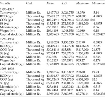
We use unique data from a survey of water-polluting industries in India.Footnote ¹¹ These survey data provide information about characteristics of India's main plants for the three financial years 1996–1997, 1997–1998 and 1998–1999. Plant-level data is appropriate since it allows us to avoid the problem of aggregation in variables. The data is provided for sales values, BOD, COD and SS pollutants, capital stocks, wage bills and other material input costs for a sample of 92 plants. The firms in the sample include leather, distillery, chemicals, sugar, paper products, fertilizers, pharmaceuticals, drugs, petrochemicals, iron and steel, refining and other industries. Sales in real 1996 values are considered a good output measure, while the three generated pollutants, BOD, COD and SS, are considered bad outputs in the estimation. Similarly, the inputs wage bill, capital stock and material costs are also taken in real 1996 values. Descriptive statistics for the variables used in the study are given in table 1. Note that in India there are water pollution standards for firms in terms of concentration ratios. A firm may be in compliance even by diluting the concentration of pollutants by increasing the amount of water used. Therefore we use pollution load which is a product of pollution concentration and the volume of wastewater in the estimation of directional output distance function. Table 1 reveals that the environmental performance of Indian manufacturing firms improved over the period 1996–1997 to 1998–1999. For example, the BOD load to turnover ratio which was about 30 in 1996–1997 came down to about 23 in 1998–1999. Similarly, the ratio of COD load to turnover and ratio of SS load to turnover came down to 158 from 210 and 45 from 60, respectively.

Table 1.

Summary statistics of the variables used in the study

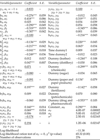
The estimated parameters for the directional output distance function are presented in table 2. We find that the ML estimation parameters are statistically significant. Most of the first-order parameters have the expected signs and are statistically significant. Looking at the second-order parameters, it appears that they reveal interesting results. These, however, require a more detailed analysis to understand their ultimate influence. Thus, using the estimated coefficients, we are able to verify that the resulting distance functions satisfy regularity conditions (monotonicity and concavity conditions) for average values. For the directional output distance function to be well behaved, it needs to be non-negative and the constraints of monotonicity,Footnote ¹² symmetry and the translation property need to hold. In a stochastic estimation of the distance functions, translation and symmetry properties are imposed, and monotonicity is tested for afterwards. The monotonicity condition implies positive marginal products, or increasing one input quantity while holding all others constant lowers the measure. We find that the monotonicity condition with respect to sales values is satisfied by most of the observations (99.64 per cent). With respect to BOD, the monotonicity condition is satisfied by 58.33 per cent of the observations. Similarly, we find that the condition of monotonicity is fulfilled by 60.61 per cent observations with respect to COD. With respect to SS, we find that the monotonicity condition was satisfied for 57.24 per cent of observations. In case of pollution, this regularity condition implies that pollution can only be reduced through increased usage of at least some inputs with constant desirable output and technology. The monotonicity condition is satisfied less in case of pollution. That is, pollution is reduced by less use of some inputs such as using less material, labor and capital. Where the monotonicity condition does not hold, producers are located on the downward-sloping segment of the frontier. In this situation producers can contribute social goods, i.e., reduce pollution, without limiting their capacity to maximize production of marketable outputs (Picazo-Tadeo and Prior, Reference Picazo-Tadeo and Prior2009).

Table 2.

Quadratic directional distance function parameter estimates

Notes: Underlined parameters were calculated using the translation property. ***, **, * indicate the coefficient is statistically different from zero at 1, 5 and 10%, respectively. y₁, sales value, b₂, BOD, b₃, COD, b₄, SS, x₁, materials, x₂, wages, x₃, capital stock.

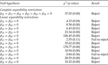
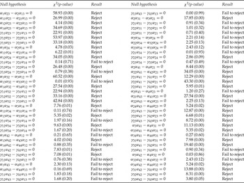
One of our major goals is to empirically test for non-separability between marketable output and pollutants, within the set of three pollutants. As outlined above, we follow Blackorby et al. (Reference Blackorby, Primont and Russell1977) to test the hypothesis of separability between outputs in a directional output distance function framework. Here, separability implies that marginal transformation rates between a pair of outputs in the separated group are independent of the levels of outputs outside the group. Separability test results are reported in tables 3a and 3b. These results lead us to reject the null hypotheses of separability between marketable output and pollutants, and between different pollutants.

Table 3a.

Tests for separability among outputs in directional output distance function (complete and linear restrictions)

Table 3b.

Tests for separability among outputs in directional output distance function (non-linear restrictions)

Note: y₁, sales value, b₂, BOD, b₃, COD, b₄.

Application of the econometric approach for estimating parameters allows us to test whether the distribution of the inefficiency term is significantly different from zero. The log-likelihood ratio test helps reject the null hypothesis of zero inefficiency, i.e., the Indian water polluting plants are not operating at the frontier P(x), on average. The inefficiency estimates of E(μ | ɛ) (i.e., the value of the directional distance function) are obtained for each observation, following Kumbakhar and Lovell (Reference Kumbakhar and Lovell2000).

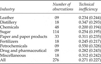
Table 4 shows industry-specific average estimates of technical inefficiency. For a representative water-polluting firm, and using the overall sample mean of inputs to produce the sample mean of outputs, the estimated value of the directional output distance function is 0.27. This indicates that production is not technically and environmentally efficient. These water-polluting firms could, on average and without changing resources or developing technology, increase sales by 516 million Indian Rupees (Rs.) (3,291.9 × 0.27) and reduce BOD, COD and SS by 13,671, 93,043 and 26,857 thousand kg, respectively. We find that the petrochemicals industry is the most inefficient, and the chemicals industry the most efficient industry in India. The reduction potential in emission by plant relates positively to water quality targets for BOD, COD and TSS where the simple correlations are 0.67, 0.71 and 0.60, respectively. We might be able to say that higher targets are associated with larger potential.

Table 4.

Estimates of technical inefficiency: means and standard deviation

The environmental constraint imposed by regulation and the production structure determine the value of the shadow price. In the directional output distance function some pollution reduction can be achieved at no cost by eliminating inefficiency. The shadow price is measured once technical inefficiency has been eliminated. Huhtala and Marklund (Reference Huhtala and Marklund2008) show the relationship between society's environmental preferences and the opportunity costs of firms at the social optimum constrained by environmental regulations. This linkage provides a theoretical explanation that the environmental constraint determines where on the production frontier the shadow price should be calculated. Understanding the point on the frontier is meaningful from an environmental perspective because the shadow price enables an evaluation of the benefit society gains from improved environmental quality with the cost (i.e., reduced output) associated with this improvement.

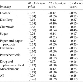
Table 5 provides estimates of industry-specific shadow prices for pollutants for observations that satisfy monotonicity conditions. These can be interpreted as the marginal abatement costs for these pollutants. These shadow prices are negative, reflecting marketable output and revenues foregone as a result of reducing the effluent by 1,000 kg. For instance, the average shadow price per thousand kg for water-polluting industries is Rs. 0.29 million for BOD, Rs. 0.12 million for COD and Rs. 0.28 million for SS. This implies that a reduction of BOD by 1,000 kg reduces production by Rs. 0.29 million worth of positive output.

Table 5.

Estimates of shadow prices (millions Indian Rs. per thousand kg) (observations satisfying monotonicity conditions)

Note: Values in parentheses are standard deviations

There is wide variation in the shadow prices of pollutants across plants and industries (see table 5). In the case of BOD, the leather industry shows the highest marginal cost of abatement. To reduce SS, the marginal abatement costs are highest in petrochemical-producing firms. Leather-producing firms must incur the highest marginal abatement costs to reduce COD. The estimates of marginal cost functions reported above can be used to design economic instruments for controlling pollution.

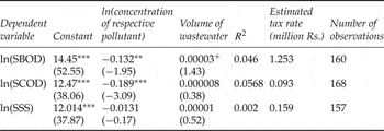
Using the taxes-standards approach (Baumol and Oates, Reference Baumol and Oates1988),Footnote ¹³ pollutant-specific pollution taxes can be designed, given the standards and the estimates of marginal abatement cost functions. In the case of water pollution, the minimum national standards (MINAS) are given as 35 μg/l for BOD, 250 μg/l for COD and 100 μg/l for SS in India (CPCB, 1995). The taxes-standards method requires the pollution tax to be fixed at the rate equal to the marginal cost of abatement corresponding to the prescribed standard. Keeping the wastewater volume at its mean level for the Indian industry and taking MINAS standards as the pollution concentrations in the equations of marginal abatement cost functions, the corresponding shadow price or the marginal cost of abatement for each pollutant can be computed. Table 6 reports the regression results of shadow prices of pollution regressed on concentration ratios and wastewater volume. As expected we find a negative relationship between the level of concentration of a pollution ratio and the marginal abatement cost. That is, as the firms want to reduce the level of pollution concentration ratio, the marginal abatement cost increases. The firms in the Indian industry can comply with the standards by levying taxes on them equal to Rs. 1.25 million, Rs. 0.93 million and Rs. 0.016 million, respectively, for a ton of BOD, COD and SS.

Table 6.

Regression results

Notes: Figures in brackets are t-statistics. ***significant at 1% level; ** significant at 5% level, ⁺significant at 15% level. SBOD, shadow price of BOD; BODC, concentration of BOD μg/l; SCOD, shadow price of COD; CODC, concentration of COD μg/l; SSS, shadow price of SS; SSC, concentration of SS μg/l.

Recall that the MES measures the relative change in shadow prices for outputs due to relative changes in output quantities. As these are indirect elasticities, the higher its value (in absolute terms), the lower is the degree of interaction between outputs. In the case of marketable output and pollutants, given the monotonicity condition, translation property and concavity of the directional distance function, the sign of Morishima substitution elasticity between a pollutant and marketable output is expected to be negative, at least if there is only a single marketable output and a single pollutant.

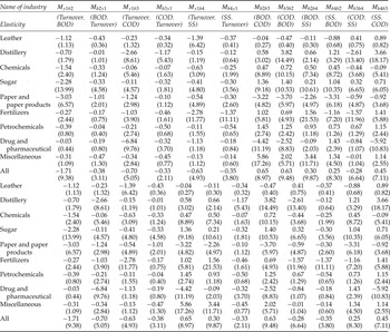
The estimates of Morishima elasticities for the observations satisfying monotonicity conditions are presented in table 7. As expected, at the average level, the signs of M₂₁, M₃₁ and M₄₁ (i.e., the Morishima substitution elasticity between the pollutants BOD, COD, SS and marketable output) are all negative. This result indicates that the reduction in any pollutant is not without costs, i.e., that firms have to incur abatement costs for reducing pollution levels. In the case of BOD, the elasticity of substitution is highest for the paper and paper product industry and lowest for distillery firms, with an overall average of −0.38. Similarly, in the case of COD, pollution reduction is least difficult for paper and paper product firms, but is more difficult for the distillery firms. The elasticity of substitution between marketable output and BOD, COD and SS varies in the ranges of −0.01 to −1.01, −0.1 to −1.17 and −0.12 to −1.37, respectively. Moreover, the results indicate that there is asymmetry in the substitution elasticity between marketable output and pollution, and between pollution and marketable output (see table 7).

Table 7.

Estimates of the Morishima elasticity of substitution (all observations)

Notes: y₁, sales value, b₂, BOD, b₃, COD, b₄. Values in parentheses are standard deviations.

The interaction between the abatement costs of different pollutants can be explained by these estimates of Morishima elasticities. The results for substitution elasticities between BOD and COD indicate that if the intensity of BOD relative to COD is reduced, the relative marginal cost of the abatement ratio between two pollutants is increased, i.e., the pollutants are substitutes for one another in the abatement process at the average level. However, in some industries (leather, paper and paper products, and drug and pharmaceutical industries) there is complementarity between these two pollutants, as the sign of the Morishima elasticity of substitution is negative. This complementarity is highest for paper and paper product firms and lowest for the drug and pharmaceutical industry. Both pollutants are types of organic water pollution, though COD also incorporates the impact of other contaminants on the rate of oxidation by microorganisms in the water. Reduction of COD may entail some reduction in BOD, which is also true in the converse (see Dasgupta et al., Reference Dasgupta, Huq, Wheeler and Zhang2001). Contrary to the relationship between these two organic water pollutants, the relationship between BOD (or COD) and SS is one of substitutability, i.e., if the intensity of BOD (or COD) relative to SS is reduced, the relative marginal cost of the abatement ratio between the two pollutants increases. We also observe asymmetry in the elasticity estimates between different pollutants.

5. Discussion and conclusions

The design and implementation of environmental policy often involve more than one pollutant. In general, each environmental policy tends to consider a single pollutant. The isolated analysis of only one pollutant may be qualitatively misleading if multiple pollutants are involved in a production activity (Moslener and Requate, Reference Moslener and Requate2007). We can consider, for example, the case where increases in the stringency of environmental regulations on one pollutant cause plants to substitute a less regulated pollutant in the production process. In addition, sound environmental policy needs to consider pollution as a by product of the production of marketable output. When environmental quality and consumption goods are non-separable elements of consumer preferences or production technologies, a change in the level of environmental quality can affect market demands (Carbone and Smith, Reference Carbone and Smith2008). Therefore, non-separability and substitutability of pollutants are crucial in considering the effect of pollution on the market economy. Earlier studies, however, often assume: (1) production of marketable output, pollution and abatement are separable; and (2) different pollutants can be abated separately.

In this study, using unique plant-level data in India with the pollutants BOD, COD and SS, we test the validity of these common assumptions. We find that the reduction of any one pollutant is not without costs and, therefore, that firms must incur abatement costs for reducing pollution levels. In addition, BOD and COD are complements to one another in the abatement process in the leather, paper and paper products, and drug and pharmaceutical industries. SS and the other pollutants, however, are substitutes.

Measures of BOD and COD measure the amount of organic compounds in water (Cheremisinoff, Reference Cheremisinoff2001). The difference is that COD is less specific, since it measures everything that can be chemically oxidized, rather than just levels of biologically active organic matter (i.e., BOD). Therefore, the relative marginal cost of the abatement ratio between the two pollutants is reduced if the intensity of BOD relative to COD is reduced.

SS refers to small solid particles that remain suspended in water as a colloid due to the motion of the water. From an engineering viewpoint, it is not clear whether SS is a complement or a substitute to other pollutants. Though all three measures are indicators of water quality, we find that relationships are different over pollutants and over industries. From a practical policy viewpoint, policy targets should not necessarily consider the three pollutants independently. Instead, it might be appropriate to combine the three into a targeted index of BOD, COD and SS to reduce monitoring costs.

No previous studies estimate the non-separability and substitutability of pollutants when considering the production processes and joint abatement of several pollutants. For example, Greenstone (Reference Greenstone2003) empirically examines the effect of reducing air pollution in the iron and steel industry, but does not consider the production side because data was not available. Our study contributes to the literature by empirically showing the importance of assuming non-separability and substitutability in economic modeling and providing policy guidance.

Footnotes

¹ We must note that this need not be based on the assumption that pollutants are abated separately. It could be because all pollutants are abated jointly, and therefore focusing on one pollutant is sufficient.

² Theoretically, Moslener and Requate (Reference Moslener and Requate2007) show cases for substitutes and complements. For substitutes, one pollutant may initially increase while another decreases along the optimal emission path. Then, both pollutants approach the steady state. For complements, this pattern is reversed. Initially, both pollutants are reduced or relaxed simultaneously. Then, there is a fine-tuning in the allocation of the two pollutants. One pollutant may approach the steady-state level from below, while the other may approach it from above.

³ Exceptions include Reynaud (Reference Reynaud2003), who considers non-separability. Reynaud (Reference Reynaud2003) investigates the water demand of French manufacturing by estimating a multiproduct translog cost function.

⁴ Baumol and Oates (Reference Baumol and Oates1988), in their seminal study, show that in the absence of information on environmental damage from pollution, predetermined environmental standards can be achieved with uniform effluent taxes. Beavis and Walker (Reference Beavis and Walker1979) show that this solution is sub-optimal when there are multiple pollutants that are simultaneously generated and abated.

⁵ Null-jointness implies that a firm cannot produce marketable outputs in the absence of pollutants, i.e., if (y, b) ∈ P(x) and b = 0 then y = 0.

⁶ For the properties of directional output distance functions, see Färe et al. (Reference Färe, Grosskopf, Noh and Weber2005).

⁷ The Morishima elasticity of substitution (MES) measures the effect of change in the price of one output to the output ratio of the same output and one other. The MES has the special feature of being asymmetric, that is M _ij ≠ M _ji, unless the directional distance function is a member of the CES–Cobb–Douglas family. Asymmetry implies that the MES evaluates the substitutability with respect to either the one or the other price. When the number of outputs exceeds two, any substitution elasticity is partial. An equal percentage change of the one or the other output price incurs different changes to the optimal output ratio, and therefore the substitution elasticity is inherently asymmetric (Blackorby and Russell, Reference Blackorby and Russell1989). When two elasticities are of opposite sign, appropriate interpretation can be provided using higher statistical significance of parameters.

⁸ However, stochastic methods have their own disadvantages, such as distributional assumptions for the inefficiency and error terms, and the problem of imposing non-linear monotonicity constraints in the estimation process.

⁹ STATA 9.0 version is used for estimating the directional output distance function. To check the sensitivity of the result with respect to the distribution of one-sided error term we tried for different distributions such as truncated normal and exponential distributions; however, the results were not qualitatively different from the half-normal distribution. Since half-normal distribution is much in practice, here we report only the results based on the assumption of half-normal distribution of one-sided error term.

¹⁰ The index value of the sales value for an observation is its sales value normalized by the industry-specific mean sales value.

¹¹ The data source for this study is ‘A survey of water polluting industries in India’, Research Project on Environmental and Economic Accounting for Industry, Institute of Economic Growth, Delhi in 2000. A sample of 1,500 plants was drawn up, giving required representation to 19 categories of water-polluting plants in India, as notified by the Central Pollution Control Board (CPCB). The questionnaire was sent to plants with a letter from the project director and the Chairman of CPCB and the Chairman of the State Pollution Control Board (SPCB). These letters were followed by letters from the project director to the offices in charge of SPCB offices at district headquarters, requesting them to follow up with the plants in their jurisdiction to provide the information asked for in the questionnaire. Finally, staff and senior officials visited SPCB offices and plants to secure filled-in questionnaires from as many plants as possible. We should note that the statistics covered in our data do not represent the entire Indian industry. In addition, our data covers mostly large plants in the industry, and most of these are the ones that comply with environmental standards or make significant efforts toward water pollution abatement. However, we believe the performance of pollution abatement activities can be well analyzed in this data because of the data's reliability.

¹² (i) D _y (x, y, b; g) ≤ 0, (ii) D _b (x, y, b; g) ≥ 0, (iii) D _yy (x, y, b; g) ≤ 0, (iv) D _by (x, y, b; g) ≤ 0.

¹³ For an earlier application of this method for Indian industry, see Murty et al. (Reference Murty, James and Misra1999), Murty and Kumar (Reference Murty and Kumar2002, Reference Murty and Kumar2004) and Murty et al. (Reference Murty, Kumar and Paul2006).

References

Anderson, C.L. (1987), ‘The production process: inputs and wastes’, Journal of Environmental Economics and Management 14: 1–12.Google Scholar

Baumol, W.J. and Oates, W.E. (1988), The Theory of Environmental Policy, 2nd edn, Cambridge: Cambridge University Press.Google Scholar

Beavis, B. and Walker, M. (1979), ‘Interactive pollutants and joint abatement costs: achieving water quality standards with effluent charges’, Journal of Environmental Economics and Management 6: 275–286.Google Scholar

Bellas, A.S. (1998), ‘Empirical evidence of advances in scrubber technology’, Resource and Energy Economics 20(4): 327–343.Google Scholar

Blackorby, C., Primont, D., and Russell, R.R. (1977), ‘On testing separability restrictions with flexible functional forms’, Journal of Econometrics 5: 195–209.Google Scholar

Blackorby, C. and Russell, R.R. (1989) ‘Will the real elasticity of substitution please stand up? (a comparison of the Allen/Uzawa and Morishima elasticities)’, American Economic Review 79(4): 882–888.Google Scholar

Burtraw, D., Krupnick, A., Palmer, K., Paul, A., Toman, M., and Bloyd, C. (2003), ‘Ancillary benefits of reduced air pollution in the U.S. from moderate greenhouse gas mitigation policies in the electricity sector’, Journal of Environmental Economics and Management 45(3): 650–673.CrossRef Google Scholar

Carbone, J.C. and Smith, V.K. (2008), ‘Evaluating policy interventions with general equilibrium externalities’, Journal of Public Economics 92: 1254–1274.Google Scholar

Carlson, C., Burtraw, D., Cropper, M., and Palmer, K. (2000), ‘Sulfur dioxide control by electric utilities: what are the gains from trade?’, Journal of Political Economy 108(6): 1292–1326.Google Scholar

Cheremisinoff, N.P. (2001), Handbook of Pollution Prevention Practices (Environmental Science and Pollution Control Series), Cambridge: Marcel Dekker Inc.Google Scholar

Coelli, T., Lauwers, L., and Van Huylenbroeck, G. (2007), ‘Environmental efficiency measurement and the materials balance condition’, Journal of Productivity Analysis 28: 3–12.Google Scholar

Considine, T.J. and Larson, D.F. (2006), ‘The environment as a factor of production’, Journal of Environmental Economics and Management 52 (3): 645–662.Google Scholar

CPCB (1995), Standards for Pollution Control, Central Pollution Control Board, Delhi: Government of India.Google Scholar

Dasgupta, S., Huq, M., Wheeler, D., and Zhang, C. (2001), ‘Water pollution abatement by Chinese industry: cost estimates and policy implications’, Applied Economics 33: 547–557.Google Scholar

Dellink, R.B. (2005), Modelling the Costs of Environmental Policy: A Dynamic Applied General Equilibrium Assessment, Cheltenham/Northampton: Edward Elgar.CrossRef Google Scholar

Domazlicky, B.R. and Weber, W.L. (2004), ‘Does environmental protection lead to slower growth in the chemical industry?’, Environmental and Resource Economics 28: 301–324.CrossRef Google Scholar

Eskeland, G.S. (1997), ‘Air pollution requires multi pollutant analysis: the case of Santiago, Chile’, American Journal of Agriculture Economics 79: 1636–1641.Google Scholar

Färe, R., Grosskopf, S., Lovell, C.A.K., and Yaisawarng, S. (1993), ‘Derivation of shadow prices for undesirable outputs – a distance function-approach’, Review of Economics and Statistics 75(2): 374–380.Google Scholar

Färe, R., Grosskopf, S., Noh, D.-W. and Weber, W.L. (2005), ‘Characteristics of a polluting technology: theory and practice’, Journal of Econometrics 126(2): 469–492.Google Scholar

Fujii, H., Kaneko, S., and Managi, S. (2010), ‘Changes in environmentally sensitive productivity and technological modernization in China's iron and steel industry in the 1990s’, Environment and Development Economics 15(4): 485–504.Google Scholar

Goldar, B.N., Misra, S., and Mukherji, B. (2001), ‘Water pollution abatement cost function: methodological issues and an application to small-scale factories in an industrial estate in India’, Environment and Development Economics 6: 103–122.CrossRef Google Scholar

Greene, W. (1993), ‘The econometric approach to efficiency analysis’, in Fried, H., Lovell, C.A.K. and Schmidt, S. (eds), The Measurement of Productive Efficiency, Oxford: Oxford University Press, p. 68–119.Google Scholar

Greenstone, M. (2003), ‘Estimating regulation-induced substitution: the effect of the Clean Air Act on water and ground pollution’, American Economic Review 93(2): 442–448.Google Scholar

Huhtala, A. and Marklund, P.O. (2008), ‘Stringency of environmental targets in animal agriculture: shedding light on policy with shadow prices’, European Review of Agricultural Economics 35: 193–217.Google Scholar

Kumbakhar, S. and Lovell, C.A.K. (2000), Stochastic Frontier Analysis, Cambridge: Cambridge University Press.Google Scholar

Kolstad, C.D. and Turnovsky, M.H.L. (1998), ‘Cost functions and nonlinear prices: estimating a technology with quality-differentiated inputs’, Review of Economics and Statistics 80(3): 444–453.CrossRef Google Scholar

Kumar, S. and Managi, S. (2009), ‘Energy price-induced and exogenous technological change: assessing the economic and environmental outcomes’, Resource and Energy Economics 31(4): 334–353.Google Scholar

Kumar, S. and Managi, S. (2010), ‘Environment and productivities in developed and developing countries: the case of carbon dioxide and sulfur dioxide’, Journal of Environmental Management 91(5): 1580–1592.Google Scholar

Kuper, G.H. and Van Soest, D.P. (2003), ‘Path-dependency and input substitution: implications for energy policy modelling’, Energy Economics 25(4): 397–407.Google Scholar

Managi, S., Opaluch, J.J., Jin, D., and Grigalunas, T.A. (2005), ‘Environmental regulations and technological change in the offshore oil and gas industry’, Land Economics 81(2): 303–319.Google Scholar

Montero, J.-P. (2001), ‘Multipollutant markets’, RAND Journal of Economics 32(4): 762–774.Google Scholar

Moslener, U. and Requate, T. (2007), ‘Optimal abatement in dynamic multi-pollutant problems when pollutants can be complements or substitutes’, Journal of Economic Dynamics and Control 31: 2293–2316.Google Scholar

Murty, M.N., James, A.J., and Misra, S. (1999), Economics of Water Pollution: The Indian Experience, New Delhi: Oxford University Press.Google Scholar

Murty, M.N. and Kumar, S. (2002), ‘Measuring cost of environmentally sustainable industrial development in India: a distance function approach’, Environmental and Development Economics 7: 467–486.Google Scholar

Murty, M.N. and Kumar, S. (2004), Environmental and Economic Accounting for Industry, New Delhi: Oxford University Press.Google Scholar

Murty, M.N., Kumar, S., and Dhavala, K.K. (2007), ‘Measuring environmental efficiency of industry: a case study of thermal power generation in India’, Environmental and Resource Economics 38: 31–50.Google Scholar

Murty, M.N., Kumar, S., and Paul, M. (2006), ‘Environmental regulation, productive efficiency and cost of pollution abatement: a case study of sugar industry in India’, Journal of Environmental Management 79(1): 1–9.CrossRef Google Scholar

Picazo-Tadeo, A.J. and Prior, D. (2009), ‘Environmental externalities and efficiency measurement’, Journal of Environmental Management 90: 3332–3339.Google Scholar

Reynaud, A. (2003), ‘An econometric estimation of industrial water demand in France’, Environmental and Resource Economics 25: 213–232.CrossRef Google Scholar

Schmieman, E.C, van Ierland, E.C, and Hordijk, L. (2002), ‘Dynamic efficiency with multi-pollutants and multi-targets: the case of acidification and tropospheric ozone formation in Europe’, Environmental and Resource Economics 23(2): 133–148.Google Scholar

Schwabe, K.A. (1999), ‘The effects of separability on incentive based instrument performance’, Economics Letters 63(3): 377–380.Google Scholar

Smith, V.K. (1998), ‘Should pollution reductions count as productivity gains for agriculture?’, American Journal of Agricultural Economics 80: 591–594.Google Scholar

Weaver, R.D. (1998), ‘Measuring productivity of environmentally interactive technologies’, American Journal of Agricultural Economics 80: 595–599.Google Scholar

Welch, E. and Barnum, D. (2009), ‘Joint environmental and cost efficiency analysis of electricity generation’, Ecological Economics 68(8–9): 2336–2343.Google Scholar

Wossink, G.A.A., Lansink, A.G.J.M. Oude, and Struik, P.C. (2001), ‘Non-separability and heterogeneity in integrated agronomic-economic analysis of non-point source pollution’, Ecological Economics 38: 345–357.Google Scholar

Yohe, G. (1976), ‘Substitution and the control of pollution: a comparison of effluent charges and. quantity standards under uncertainty’, Journal of Environmental Economics and Management 3: 312–324.CrossRef Google Scholar