Drake equation summary
For over half a century the acclaimed Drake equation (Drake Reference Drake1962) has provided a useful synthesis of the factors involved in the search for intelligent life. The main terms in the Drake equation are as follows (http://www.seti.org/drakeequation).
 $$N = R_{^\ast} F_{\rm p} n_{\rm e} F_{\rm l} F_i F_{\rm c} L,$$
where N, the number of communicative extraterrestrial civilizations in the Galaxy; R *, the rate of star formation in the Milky Way Galaxy; F p, the fraction of stars with planetary systems; n e, the number of potentially life-hosting planets per star; F l, the fraction of planets that develop life; F i, the fraction of life-bearing planets with intelligent life; F c, the fraction of civilizations that have developed technology that releases detectable signals into space; L, the length of time the civilization is releasing such detectable signals.
In the Drake equation, the first three terms are measureable. The star formation rate, R *, in the Milky Way Galaxy is estimated at about 1 Solar mass worth of stars per year (Chomiuk & Povich Reference Chomiuk and Povich2011). The fraction of stars with planets or planetary systems, F p, is an intense ongoing research area (Winn & Fabrycky Reference Winn and Fabrycky2015); see the section ‘Fraction of stars with planets’ for more details.
The number of potentially life-hosting planets per star, n e, is the one that astronomers have been working on, by way of occurrence studies of ‘habitable zone’ planets. The habitable zone is the zone around a star where a rocky planet with a thin atmosphere, heated by its star, may have liquid water on its surface. While we have estimates of the occurrence of Earth-size planets in the habitable zone of different host star types, these are not yet secure for Earth-like planets orbiting sun-like stars (see the section ‘Fraction of stars with planets’).
There is some hope we might have an estimate for F l in the next decades, or century, if life is common and we are able to detect biosignature gases (see the section ‘The search for biosignature gases’).
All of the other terms in the Drake equation are not measureable and arguably never will be. We emphasize that the Drake equation is not intended as a prediction but as a summary of the main concepts that go into the question of detecting signals from intelligent life in the Galaxy, rather than any estimate of the number of intelligent extraterrestrial civilizations in the galaxy. For the original description of the Search for Extra-Terrestrial Intelligence (SETI) see Cocconi & Morrison (Reference Cocconi and Morrison1959) and (Drake Reference Drake1961), for a detailed description of the history and context of SETI see Tarter (Reference Tarter2001) and for a retrospective by Frank Drake see Drake (Reference Drake2013). For information on the recent resurgence of SETI funding in the form of a 10 year, $100 million initiative, see http://breakthroughinitiatives.org/Initiative/1.
A ‘Biosignature Drake Equation’ for the number of planets with detectable signs of life
Equation overview
The search for life beyond the solar system by way of biosignature gases in exoplanet atmospheres has accelerated towards reality in recent years, warranting a new kind of descriptive equation. While ‘listening’ for radio communications was possible decades ago, the search for biosignature gases is only possible in the near future because of the recent discoveries establishing the existence of small rocky exoplanets and new telescopes under construction (see the section ‘The search for biosignature gases’).
There is, therefore, a motivation for a revised Drake equation, which I call the ‘Biosignature Drake Equation’, a copy and extension of the original Drake equation but as applied to the conventional astronomical search for life.
In the fashion of the Drake Equation, we may estimate the number, N, of planets with detectable signs of life by way of biosignature gases
 $$N = N_{^\ast} F_{\rm Q} F_{{\rm HZ}} F_{\rm O} F_{\rm L} F_{\rm S}, $$
where N *, the number of stars in the survey; F Q, the fraction of stars in the survey that are suitable for planet finding (e.g., quiet non-variable stars or non-binary stars); F HZ, the fraction of stars with rocky planets in the habitable zone; F O, the fraction of those planets that can be observed, according to limitations of planet orbital geometry or other limiting factors; F L, the fraction of planets that have life; F S, the fraction of planets with life that produces a detectable biosignature gas by way of a spectroscopic signature.
Like the Drake Equation, the revised Biosignature Drake Equation is useful to help describe the search rather predict an outcome; the first four terms are measureable or quantifiable, but the last two are not.
One may ask why separating out F Q and F O, when they could be lumped in with the number of stars in the survey N *. The reason is that each term elucidates an important issue. For F Q, the issue is that out of the stars in a volumetric or otherwise finite set of stars, there are always a fraction of stars that are not amenable for observation (such as variable or binary stars). For F O, the issues may relate to planet orbital geometry – the planet is not visible at all or all of the time, depending on the search method.
Equation application to Transiting Exoplanet Survey Satellite/James Webb Space Telescope (TESS/JWST)
The Biosignature Drake Equation is best explained by a detailed example. Let us consider the upcoming NASA TESS mission (Ricker et al. Reference Ricker2015), scheduled for launch in 2018. TESS will survey nearby stars for transiting exoplanets. Transiting exoplanets are those that pass in front of their parent star as seen from the telescope, a phenomena that is exploited as a planet discovery technique that NASA's Kepler mission (Borucki et al. Reference Borucki2010) (as well as many other surveys) has been used to discover more than 4600 exoplanets or planet candidates. TESS is an NASA Explorer-class mission ($230 million US cost cap exclusive of launch costs) led by the Massachusetts Institute of Technology. TESS will carry four identical specialized wide-field charge-coupled device cameras, each covering 24° × 24° on the sky with a 100-mm aperture. In a 2-year all-sky survey of the Solar neighbourhood, TESS will cover 400 times as much sky as Kepler did. In the process, TESS will examine more than 0.5 million bright nearby stars and likely find thousands of exoplanets with orbital periods (i.e., years) up to about 50 days. TESS will not be able to detect true Earth analogs (that is, Earth-sized exoplanets in 365 day orbits about sun-like stars), but it will be capable of finding Earth-sized and super Earth-sized exoplanets (defined as planets up to 1.75 times Earth's size) transiting M stars, stars that are significantly smaller, cooler and more common than our Sun. The TESS search for habitable planets that may be followed up for signs of life is, therefore, focused on M dwarf host stars.
The suitable number of M dwarf stars in the TESS all-sky survey is estimated to be about N * = 30 000 (from Galactic models based on M dwarf star surveys; (Reid & Hawley Reference Reid and Hawley2004; Bochanski et al. Reference Bochanski, Munn, Hawley, West, Covey and Schneider2007). Out of these M dwarf stars, about F Q ≈ 60% are expected to be quiet enough (that is not highly variable in brightness) for small planet detection. This number is very approximate and estimated from Ciardi et al. (Reference Ciardi2011), who quantify the variability of M dwarf and other stars by dispersion as a function of different timescales, based on the first quarter Kepler data. The fraction of rocky planets in the habitable zone about M stars is about F HZ = 24% (Dressing & Charbonneau Reference Dressing and Charbonneau2015); for more detail see the section ‘Fraction of stars with planets’. The transit geometry limits the fraction of stars with planets that can be observed by TESS to be about 10% and only about 1% of the initial set of stars will be bright enough for the planet's atmosphere to be observed in detail (Deming et al. Reference Deming2009), in other words we have F O = 0.1% or 0.001. Putting all of the above numbers for the first four terms in equation (2), we have: N * F QF HZF O ≈ 4. We can also summarize the discussion so far as N ≈ 4 F LF S.
An important note is that very detailed calculations of the TESS planet yield – essentially the product of the first four terms of equation (2) – are provided in Sullivan et al. (Reference Sullivan2015). There, a value of between 2 and 7 is reported. (More specifically ‘Approximately 48 of the planets with R < 2 R Earth lie within or near the habitable zone; between 2 and 7 such planets have host stars brighter than K S = 9’.)
With the pool of TESS Earth and super-Earth sized planets, extensive follow-up observations by worldwide ground-based observatories will then be used to lead to measurements of the planet mass to confirm the exoplanets as being rocky. As an important aside, we call a planet rocky if it is predominately made of silicates or iron and has a thin atmosphere not contributing much to the planet volume; theoretical calculations support this number as being 1.75 Earth radii or smaller (e.g., Valencia et al. Reference Valencia, O'connell and Sasselov2006; Seager et al. Reference Seager, Kuchner, Hier-Majumder and Militzer2007; Swift et al. Reference Swift2012; Zeng & Sasselov Reference Zeng and Sasselov2013). Measured masses and radii of dozens of small exoplanets were used to support the cutoff observationally and found that planets smaller than 1.6 Earth radii are rocky (Weiss & Marcy Reference Weiss and Marcy2014; Rogers Reference Rogers2015). While the observed value should be adopted, the fidelity of the difference between 1.6 and 1.75 Earth radii is not used in this paper's estimate.
We now turn to the discussion involving the terms F L and F S. NASA's JWST (Gardner et al. Reference Gardner2006), scheduled to launch in 2018, will be capable of studying the atmospheres of a subset of the TESS rocky exoplanets in visible, near-infrared (IR) and IR. The technique that JWST will use is called transit transmission spectroscopy. As a transiting exoplanet passes in front of its host star, we can observe the exoplanet's atmosphere as it is backlit by the star (Seager & Sasselov Reference Seager and Sasselov2000; Seager Reference Seager2010). Additional atmospheric observations can be made by observing as the exoplanet disappears and reappears from behind the star. In these observations, the exoplanets and their stars are not spatially separated on the sky but instead, observed in the combined light of the planet–star system.
We must guess at the fraction of habitable-zone planets that have life. Here we must consider that not all planets in the habitable zone will be able to support life (e.g., the surface temperature depends on the unknown greenhouse properties of the atmosphere) and we do not know how often life actually arises. Let us be optimistic, with F L = 50%. Does life generate gases that can accumulate in the planet atmosphere and are spectroscopically detectable? Let us speculate that F S ≈ 50%. To support this speculation we might consider that remotely detectable oxygen has existed in Earth's atmosphere for about half of its life (several lines of geological and geochemical evidence indicate that the level of atmospheric oxygen was extremely low before 2.45 billion years ago but reached considerable levels by 2.22 billion years ago (Bekker et al. Reference Bekker2004)).
To summarize, we have assigned the following values: N * = 30 000, F Q = 0.6, F HZ = 0.24, F O = 0.001, F L = 0.5, F S = 0.5. These values, multiplied together, yield the number of planets with detectable signs of life from the TESS/JWST combination that is N ~ 1. I have tweaked the numbers of the unknown parameters F L = 0.5, F S = 0.5 to yield the N ~ 1 favourable yet weak result – my way of stating is that we have to get very, very lucky to observing biosignature gases in the coming decade.
We can, however, state emphatically that the TESS/JWST combination is our first chance in human history with the capability to search for signs of life by way of biosignature gases on rocky exoplanets.
With the appropriate inputs, the method described in this section could be applied to other planet transit detection surveys focused on M dwarf star surveys, such as MEarth (Nutzman and Charbonneau Reference Nutzman and Charbonneau2009, Charbonneau et al. Reference Charbonneau2009) and Trappist (Gillon et al. Reference Gillon2016). The Trappist-1 system (Gillon et al. Reference Gillon2017) has seven exoplanets orbiting a a very low-mass host star, three or more of which have chance to be in the star's habitable zone, depending on the unknown atmospheric properties. Two of the planet's atmospheres were observed with the Hubble Space Telescope (de Wit et al. Reference De Wit2016) yielding a flat transmission spectrum with no clues about planet habitability. The Trappist-1 planets are suitable targets for the JWST, bolstering our hopes in the search for life by way of biosignature gases.
Equation application to ground-based direct imaging
Transiting planets are just the first part of a long story. Because of their fortuitous alignment, transiting planets are rare. After the TESS/JWST combination we look forward to the next-generation telescopes, which will use direct imaging to find and characterize (or characterize already known) planets. Direct imaging can in principle detect planets with orbits of any orientation. Atmospheres of directly imaged planets can be observed, as long as the discovery telescope has the appropriate instrumentation. First, we consider ground-based direct imaging followed by space-based direct imaging.
For both ground-based and space-based direct imaging searches, equation (2) may be used, but with different meanings for F Q and F O than in our first example for transiting exoplanets. For direct imaging, the number of stars is limited (captured in the term F Q) because binary stars may be a problem (but c.f. the below subsection) but stellar variability is not. For direct imaging, F O can be used to capture a quantifiable complication relating to observation limitations. The observational limitations can be separated into two categories, photometric and obscurational. Photometric limitations are because the planet is not always bright enough to be seen, as the planet goes through reflected light illumination phases that reduce its total brightness with respect to its ‘full’ phase (‘photometric incompleteness’). Second is a geometric limitation: as the planet orbits the star, the projected planet-star separation on the sky is changing, depending on the planet's orbital inclination. Often the planet is too close to the star as projected on the sky to be separated spatially from the star by telescope. In other words, the star obscures the planet (‘obscurational completeness’).
The large ~30 m ground-based telescopes under construction include the European Large Telescope (ELT), the Giant Magellan Telescope (GMT) and the Thirty Meter Telescope (TMT) (hereafter E-ELTs). Each of these has the opportunity to directly image planets orbiting in the habitable zones of M dwarf stars, with an instrument that can use the internal coronagraph along with adaptive optics. Although none of the E-ELTs yet has suitable ‘first light’ instruments planned, the community is working towards second generation instrumentation.
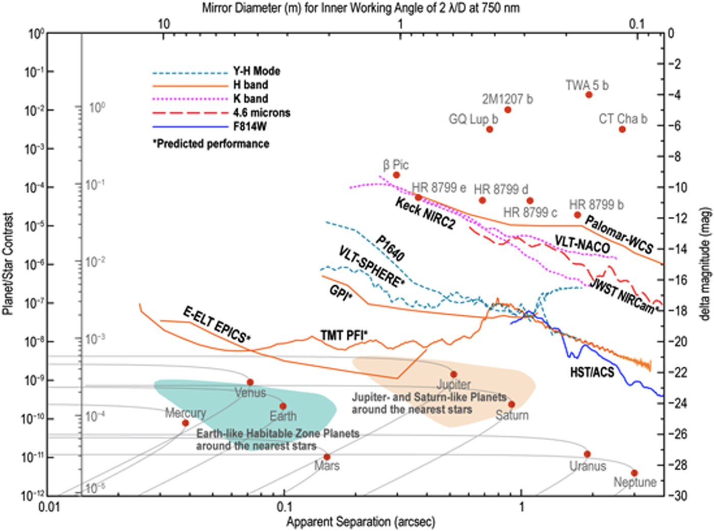
M dwarf stars are relatively bright at near-IR wavelengths as compared with visible wavelengths and hence their planets are also relatively bright in reflected near-IR light. Because the M dwarf star's habitable zone is closer to the star than that of a sun-like star, the reflected light signal is higher for the M star planet because of the 1 distance−2 fall of flux from the star. Habitable-zone planets around late M dwarf stars are detectable at ~10−7 contrast in reflected light at near-IR wavelengths (Note that habitable planets around M5 dwarf stars would have a contrast around 10−8). Even though the habitable zone for nearby late M-dwarf stars subtend very small angles (<40 mas) the ~30-m diameter telescopes will be capable of spatially resolving the planets from their host stars, with the appropriate instrumentation (see Fig. 1).
Direct imaging contrast capabilities of current and future instrumentation. Shown are the 5-σ contrast limits after post-processing of 1 h worth of data for various coronagraph instruments. As can be seen in the plot, there are roughly three groupings of curves: (1) state-of-the art instruments in the early 2010s, as represented by Keck NIRC2, the Palomar Well-Corrected Subaperture and VLT-NACO; (2) newly operational state-of-the-art instruments, represented by P1640, GPI and VLTI-SPHERE; and (3) future extremely large telescopes, represented by TMT PFI and E-ELT EPICS. The contrast curves for JWST NIRCam and HST/ACS are shown for reference. On the top right of the figure are plotted the K-band contrasts of some of the giant exoplanets imaged to date. In the lower part of the figure are plotted our Solar System planets as they would appear in reflected light around a sun-like star at a distance of 10 pc. On the left-hand side of the plot is shown the corresponding RMS wavefront error for a coronagraph using a 64 × 64 element deformable mirror. The grey region in the lower left region of the figure shows the predicted locus of terrestrial habitable zone planets for F–G–K (Solar-like) stars. Figure and caption taken from the Exo-S Final Report4 and originally adapted from (Lawson et al. Reference Lawson2012; Mawet et al. Reference Mawet2012) and Stapelfeldt (private communication Reference Stapelfeldt2015).

We take a list of M dwarf stars closer to Earth than 10 pc from the Guyon nearby star list (http://www.naoj.org/staff/guyon/04research.web/14hzplanetsELTs.web/catalog.web/content.html) (a list itself merged from six catalogs: SUPERBLINK, CNS3, 2MASS, HIPPARCOS, HIPPARCOS doubles, RECONS). There are N * = 274 M stars within 10 pc as based on the Guyon list. Out of these about 14% are stars in multiple star systems and too challenging for starlight suppression which means we set F Q = 0.86. The fraction of stars with rocky habitable-zone planets in the habitable zone is again taken from Dressing & Charbonneau (Reference Dressing and Charbonneau2015) as F HZ = 0.24. For the fraction observable, F O, we will take the fraction in the list of single M dwarf stars that have a favourable estimated planet-star contrast of 10−7 (as given in the Guyon star list), F O = 0.2. Putting all of the above estimates in my description for the first four terms in equation (2), we have: N * F QF HZF O ≈ 11, or, N ≈ 11 F LF S. If we take the optimistic numbers the fraction of planets with life F L = 50% and the fraction of life that generates spectroscopically detectable gases as F S = 50%, as before, we have N ~ 3.
The recently discovered radial velocity planet orbiting in the habitable zone of Proxima Centauri b (Anglada-Escudé et al. Reference Anglada-Escudé2016) is an incredible first planet in the category that can be studied by the ELTs with the appropriate instrumentation. In exoplanets, where there is one type of planet, there are many more and so the community is galvanized by the Proxima Centauri b discovery.
Equation application to space-based direct imaging
The Earth–Sun analogue motivates my third and final example because it is the most challenging: the Earth is 10 billion times fainter than the sun at visible wavelengths, where sun-like stars are brightest. The only way we have to starlight suppress to that level of contrast at the angular separation of Earth-sun analogue with a reasonable size telescope mirror, is in space, above the blurring effects of Earth's atmosphere. Despite their promise for M dwarf star planets, the ground-based ELTs are not expected to be able to reach the performance required for reflected light detection for Earth like planets in Earth-like orbits in a survey of sun-like star hosts out to ~10 pc (see Fig. 1).
We therefore now turn to space-based direct imaging. Starlight suppression techniques under development include the internal coronagraph and the starshade (also sometimes called the external occulter). The two concepts are far along in their development to reach the required contrast and are extremely well fleshed out in the NASA-sponsored Probe-Class Mission Reports (http://exep.jpl.nasa.gov/stdt/Exo-S_Starshade_Probe_Class_Final_Report_150312_URS250118.pdf, http://exep.jpl.nasa.gov/stdt/Exo-C_Final_Report_for_Unlimited_Release_150323.pdf) and summarized in two companion papers (Seager et al. Reference Seager2015; Stapelfeldt et al. Reference Stapelfeldt2015). The coronagraph has a technology demonstration planned by way of the inclusion of the Coronagraph Instrument (CGI) on the Wide Field Infrared Space Telescope (WFIRST), which will make possible the first images of solar system-like planets and comprehensive characterization of planets down to the size of mini-Neptunes (see, e.g., Noecker et al. Reference Noecker, Zhao, Demers, Trauger, Guyon and Jeremy Kasdin2016). The Starshade Rendezvous mission detailed in the Probe study, would launch to rendezvous on orbit with the WFIRST spacecraft and be able to reach down to Earth-like planets in the habitable zones of sun-like stars.
We take a list of FGK stars closer than 10 pc from the Guyon nearby star list. There are N * = 81 FGK stars within 10 pc as based on the Guyon list. Out of these about 20% are stars in binary systems and too challenging for starlight suppression which means we set F Q = 0.8. Note that the coronagraph starlight suppression technique may be able to handle binary stars (Thomas et al. Reference Thomas, Belikov and Bendek2015), and two starshades working together also have potential (S. Shaklan (private communication 2017)). The fraction of stars, in this case, sun-like stars with rocky habitable-zone planets in the habitable zone is not actually known; but see the section ‘Fraction of stars with planets’ for details. I will take F HZ = 0.1. Let us adopt F O = 2/3, meaning that the obscurational and photometric completeness means the space-based starlight-suppression capable observatory can observe a combined 2/3 of all habitable zones. Putting all of the above estimates in my description for the first four terms in equation (2), we have: N * F QF HZF O ≈ 4, or, N ≈ 4 F LF S.
We emphasize that very detailed calculations in the form of a ‘Design Reference Mission’ are carried out in numerous studies for the coronagraph and starshade (Dmitry et al. Reference Dmitry, Kasdin and Eric2010; Stark et al. Reference Stark, Roberge, Mandell and Robinson2014; Trabert et al. Reference Trabert, Shaklan and Lisman2015). These calculations specifically include the photometric and obscurational completeness per individual star, sun and Earth constraints for specific observing dates, telescope parameters and most importantly observation strategy (such as number of revisits per target star). Ultimately the detailed calculations are folded into the goal of calculating planet yield and for example, for the Starshade Rendezvous Mission are reported in the Probe Study equivalent to N ≈ 5 F LF S for a 2-year survey with single visits, anticipating a third year for confirmation and follow-up observations.
As in our prior applications of the Biosignature Drake Equation, we must guess at the fraction of habitable planets that have life. Let us take the same optimistic values, with the fraction of planets with life to be F L = 50% and the fraction of life that generates spectroscopically detectable gases as F S = 50%.
To summarize, we have assigned the following values: N * = 81, F Q = 0.8, F HZ = 0.1, F O = 0.67, F L = 0.5, F S = 0.5. These values, multiplied together, yield the number of planets with detectable signs of life from space-based direct imaging concepts is N ≈ 1.
To increase the numbers, the astronomy community will ultimately need to go for improvements over the Probe Study concepts, possibly by a larger starshade to go with WFIRST and to even larger telescopes and larger and possibly multiple starshades, with such topics being considered under the current NASA-sponsored pre-Decadal Studies HabEx (http://www.jpl.nasa.gov/habex/) and LUVOIR (http://asd.gsfc.nasa.gov/luvoir/) (and see also the recent AURA HDST Report (http://www.hdstvision.org), Dalcanton et al. Reference Dalcanton2015).
The fact remains that space telescopes, above the blurring effects of Earth's atmosphere are needed for the first search for rocky planets with signs of life for Earth-size planets in orbiting in the habitable zones of sun-like stars.
The search for biosignature gases
Here we review and discuss the search for biosignature gases, by focusing on two issues key to the search for biosignature gases (and included in the Biosignature Drake Equation), the fraction of stars with planets and current thinking on biosignature gases.
Fraction of stars with planets
The fraction of stars with planets, F p, is an intense topic of recent study, as it is a parameter finally within reach. Deriving the percentage of stars that host planets is not straightforward; one cannot simply divide the number of planets detected by the number of stars observed. All of the possible observational biases have to be accounted for to consider planets not discovered but might have been without the biases. The main conclusions for F p have been drawn from the treasure trove of Kepler Space Telescope (Borucki et al. Reference Borucki2010) data on transiting planets (Fressin et al. Reference Fressin2013; Howard Reference Howard2013). Planet statistics for transiting planets are supplemented by radial velocities and microlensing surveys (Sumi et al. Reference Sumi2010; Cassan et al. Reference Cassan2012).
The fraction of stars with rocky planets in the habitable zone (F HZ in the Biosignature Drake Equation and related to n e, the number of potentially life hosting planets per star in the Drake Equation) is a term where some progress has been made in recent years. A robust statement,  $15_{ - 2.7}^{ + 1.8} $% of solar type stars – roughly one in six – has a 1–2 Earth size planet P = 5–50 days (Petigura et al. Reference Petigura, Marcy and Howard2013). This is interior to the habitable zone, however and extrapolating beyond, to the habitable zone, is tricky because there are no anchor points; Kepler did not discover any one Earth radius planets in the habitable zone of a sun-like star (although Kepler did find habitable zone planets around K stars and some rocky planet candidates around G stars (a few planet candidates with 1.5–2 Earth radii sizes with large error bars (Kane et al. Reference Kane2016)). A variety of studies, nonetheless, report on the occurrence ratesFootnote 1 of rocky planets in the habitable zones and report values ranging from 2 to 20% with large uncertainty and with some sensitivity on the details of the habitable zone definition (i.e., orbital period or semi-major axis range) and the range of planet radii adopted as Earth-like (Petigura et al. Reference Petigura, Marcy and Howard2013; Foreman-Mackey et al. Reference Foreman-Mackey, Hogg and Morton2014; Burke et al. Reference Burke2015; Silburt et al. Reference Silburt, Gaidos and Wu2015). The reported values typically have large uncertainties about half as large as the value, owing to uncertainties in the extrapolation to the planets of Earth-size in orbits receiving the same amount of stellar irradiation as Earth does from the sun.
The occurrence rate of Earth-sized planets in the habitable zones of M-dwarf stars (relevance to the TESS/JWST combination; see the section ‘Equation overview’) is also based on the Kepler data set range from about 0.15–0.5 with large uncertainties. The value is  $0.16_{ - 0.07}^{ + 0.16} $ Earth-sized planets per M star (defined as 1–1.5 R Earth) and a habitable zone definition scaled to M stars (and equivalent of 0.99–1.7 AU for the sun) and increases to
 $0.24_{ - 0.08}^{ + 0.18} $ planets per star for a broader habitable zone recent Venus and early Mars (Dressing & Charbonneau Reference Dressing and Charbonneau2015). M-dwarf occurrence rate estimates derived from radial velocity measurements are at the high end of this range, but broadly consistent with the values derived from Kepler data (see a summary in Dalcanton et al. Reference Dalcanton2015).
Spectroscopic gases produced by life
The term F S = the fraction of life, which produces a detectable biosignature gas, captures the notion that not all life will produce a biosignature gas. A biosignature gas is a gas produced by life that can accumulate to detectable levels in an exoplanet atmosphere.
It is worth reviewing a few of the main, emerging thoughts in research on biosignature gases. Most of the following topics are reviewed in more detail in Seager & Bains (Reference Seager and Bains2015).
Oxygen as the favoured biosignature gas but with many false positive scenarios
Oxygen (O2) is considered Earth's most robust biosignature gas (Owen, Reference Owen and Papagiannis1980; Léger et al. Reference Léger, Mariotti, Mennesson, Ollivier, Puget, Rouan and Schneider1996). O2 is present in Earth's atmosphere to 21% by volume. O2 is a reactive gas with a short atmospheric lifetime that without continual replenishment by photosynthesis in plants and bacteria would be present only in trace amounts in Earth's atmosphere, ten orders of magnitude less than present today (Kasting & Catling Reference Kasting and Catling2003; Zahnle et al. Reference Zahnle, Claire and Catling2006). Any exoplanetary observer seeing O2 in Earth's spectrum would know that some very exotic, non-geological chemistry must be producing it, hence the foundational paradigm of O2’s robustness of an exoEarth biosignature gas. There is no precise explanation for Earth's value of O2 atmospheric abundance (other than the general explanation that we have high atmospheric O2 because of a combination of the presence of photosynthesizing life and the burial of some of that life as carbon). However, there is an upper limit of plausible O2 due to run-away fires and a lower limit for large-scale survival of macroscopic organisms, though the latter limit is softer. Lenton & Watson (Reference Lenton and Watson2000) give the expected range of O2 to be between 18 and 25%. For a further summary see, e.g., Seager & Bains (Reference Seager and Bains2015).
There has been a prolific set of studies on O2 false positives, with the canonical example of the runaway green house where water photodissociates with H escaping to space, enabling O2 to accumulate to detectable levels (Kasting Reference Kasting1988; Schindler & Kasting Reference Schindler and Kasting2000). The others fall into a variety of scenarios, some with weak atmosphere or surface sinks for O2 such that any abiotic production can enable O2 to accumulate (Selsis et al. Reference Selsis, Despois and Parisot2002; Léger et al. Reference Léger, Fontecave, Labeyrie, Samuel, Demangeon and Valencia2011; Hu et al. Reference Hu, Seager and Bains2012; Domagal-Goldman et al. Reference Domagal-Goldman, Segura, Claire, Robinson and Meadows2014; Wordsworth & Pierrehumbert Reference Wordsworth and Pierrehumbert2014; Harman et al. Reference Harman, Schwieterman, Schottelkotte and Kasting2015; Luger & Barnes Reference Luger and Barnes2015).
Many false-positive scenarios will require the environmental context via broad-wavelength, high spectral resolution or otherwise detailed enough spectral data. Detection of highly saturated water vapour, for example, would help identify the runaway greenhouse scenario. Broad wavelength, high-spectral resolution observations, may be too challenging, in one example because of the number of observing modes of JWST needed to cover the wavelength range of interest and the time consuming observations for small planets that by definition will have weak signals. In other words, for any future detection, we have to ask if the data quality is sufficient to unambiguously identify O2 and other atmospheric gases, which would set the environmental context in which we are confident that the O2 is not being geochemically or photochemically generated.
Thermodynamic disequilibrium
The earliest suggestion for the search for life beyond Earth was for a search for materials substantially out of thermodynamic equilibrium (Lederberg Reference Lederberg1965; Lovelock Reference Lovelock1965), specifically the combination of hydrocarbons and molecular oxygen on the Earth's atmosphere (a redox disequilibrium). The concept of methane (CH4) as the hydrocarbon to be contrasted with O2 became an early mainstay in biosignature gas research (Lippincott et al. Reference Lippincott, Eck, Dayhoff and Sagan1967).
There are several arguments against the use of thermodynamic equilibrium [summarized in Seager & Bains (Reference Seager and Bains2015)]. The first is observational. In practice, it could be difficult to detect both molecular features of a redox disequilibrium pair. For example, Earth was not oxygenated during early times when methane may have been abundant [by methanogens; Haqq-Misra et al. (Reference Haqq-Misra, Domagal-Goldman, Kasting and Kasting2008)], yet during present times CH4 features are likely too weak to be observed by the first generation of space-based observatories capable of finding and studying an Earth-like exoplanet. The second argument against thermodynamic disequilibrium as a life indicator relates to false positives – significant thermodynamic disequilibrium can be generated by geochemical or photochemical processes. For example, volcanism produces both SO2 and H2S, a gas mixture out of thermodynamic equilibrium at terrestrial surface conditions. The third argument against thermodynamic equilibrium is that the state of a terrestrial planet atmosphere is ill defined such that all terrestrial solar system planet atmospheres appear to be out of thermodynamic equilibrium even without the presence of life (Krissansen-Totton et al. Reference Krissansen-Totton, Bergsman and Catling2015).
A plethora of biosignature gas possibilities
To maximize our chances of recognizing biosignature gases, we promote the concept that all stable and potentially volatile molecules should initially be considered as viable biosignature gases (Seager et al. Reference Seager, Bains and Petkowski2016). Each gas would have to be modelled in context of its chemical lifetime in an observed or theorized exoplanet atmosphere, complete with environmental context. The motivation for considering all volatiles is twofold.
First, most gases produced by life on are produced for a variety organism-specific reasons such as stress and signalling. While most of these gases are produced in too small quantities to be accumulated to any significant level in Earth's atmosphere, conditions on other planets, including the surface sinks and sources and ultraviolet (UV) environment may allow accumulation (e.g. CH3Cl on planets orbiting low UV radiation M stars; Segura et al. Reference Segura2005). For a discussion of the classes of biosignature gases on Earth see Seager et al. (Reference Seager, Bains and Hu2013). We note that biosignature gases that are relatively abundant in Earth's atmosphere (aside from O2, discussed above), (e.g. CH4, N2O, H2S) are expected to be abundant because they are produced from chemical energy gradients, but also rife with false positives because geochemistry has the same gases to work with as life does. So while in some environments life is needed to catalyze the reaction of the disequilibrium chemicals, in others the same reactions will be spontaneously occurring. An example is methane. Methane is a by-product of methanogenesis, but it is also released from vents at mid-ocean ridges because of hydrothermal, abiotic chemistry.
Second, life on Earth truly produces a huge array of gases. Life produces all of the gases in Earth's atmosphere (specifically the troposphere) present at the parts-per-trillion level by volume or higher, with the exception of the noble gases. Most of Earth's atmospheric gases are, of course, not unique to life and moreover life is not the dominant source of atmospheric gases for most cases. Some atmospheric gases are already a basic atmospheric constituent (e.g., N2, CO2 and H2O), or produced geologically (e.g., CH4 and H2S).
In fact, the chemicals produced by life on Earth are numbering in the hundreds of thousands (estimated from plant natural products (Gunatilaka Reference Gunatilaka and Civjan2012), microbial natural products (Sanchez et al. Reference Sanchez, Guzmán-Trampe, Ávalos, Ruiz, Rodríguez-Sanoja, Jiménez-Estrada and Civjan2012) and marine natural products (Fusetani Reference Fusetani and Civjan2012)). However, only a subset of hundreds is volatile enough to enter the atmosphere at more than trace concentrations. The point is that perhaps any one of the huge number of gases produced by life on Earth might be produced in greater quantities by life on another planet and may accumulate more easily in other planet's atmosphere than it can in Earth's atmosphere.
Work in Seager et al. (Reference Seager, Bains and Petkowski2016) presents a new and systematic approach to the subject of biosignature gases by systematically constructing lists of stable and potentially volatile molecules. An exhaustive list up to six non-H atoms is presented, totalling about 14 000 molecules. The ‘non-H atom’ construct enables a simple implementation of the structural definition of a molecule as a set of non-H atoms connected to each other by at least one bond each and the N = 6 limit is for tractability as many aspects of the search required manual intervention or inspection. About ¼ of the molecules in the list of CNOPSH molecules are produced by life.
We have additionally searched for published spectra of molecules in the lists, for the eventual assessment of biosignature gases. About 1000 molecules have some form of spectra, mostly in the form of measured laboratory values at IR wavelengths. Many of the spectra are missing information (mostly path-length) needed to derive cross-sections, the physical input parameter that can be used to calculate spectra for different molecular abundances. This combined with the point that most molecules do not have spectra means that a huge amount of work via both computations and laboratory measurements are needed to understand future biosignature gases.
To proceed, we envision taking molecules or classes of molecules and assessing first how likely they are to accumulate in an exoplanet atmosphere of a specified composition and second whether or not they are spectroscopically detectable by a remote space telescope. The first point depends on the UV radiation environment from the host star that drives photochemistry, the atmospheric composition and atmospheric mass, and the surface chemistry (including sources and sinks). Here, the goal is to take classes of molecules to determine if they are stable and can accumulate in different planetary environments by integration into existing models of planetary chemistry and photochemistry. The spectroscopic detectability relies on molecular lines or bandhead estimates, which for many molecules do not exist yet (see above paragraph). The concept for application to potential biosignature gases is illustrated in Fig. 2.
Schematic representation for the concept of considering all volatile molecules in the search for biosignature gases. The goal is to start with chemistry and generate a list of all small molecules and filter them for utility as biosignature gases. The first filter is for molecules that are stable and volatile in temperature and pressure conditions relevant for exoEarth planetary atmospheres. Further filters relate to the gas detectability, aided by its Type classification and spectroscopic characteristics. Geophysically or otherwise generated false positives must also be considered. In the ideal situation, this overall conceptual process would lead to a finite but comprehensive list of molecules that could be considered in the search for exoplanet biosignature gases, based on both atmospheric models with surface source and sink input details, as well as strengths of spectroscopic features molecules. Figure credit: S. Seager and D. Beckner. Figure originally published in (Seager & Bains Reference Seager and Bains2015).
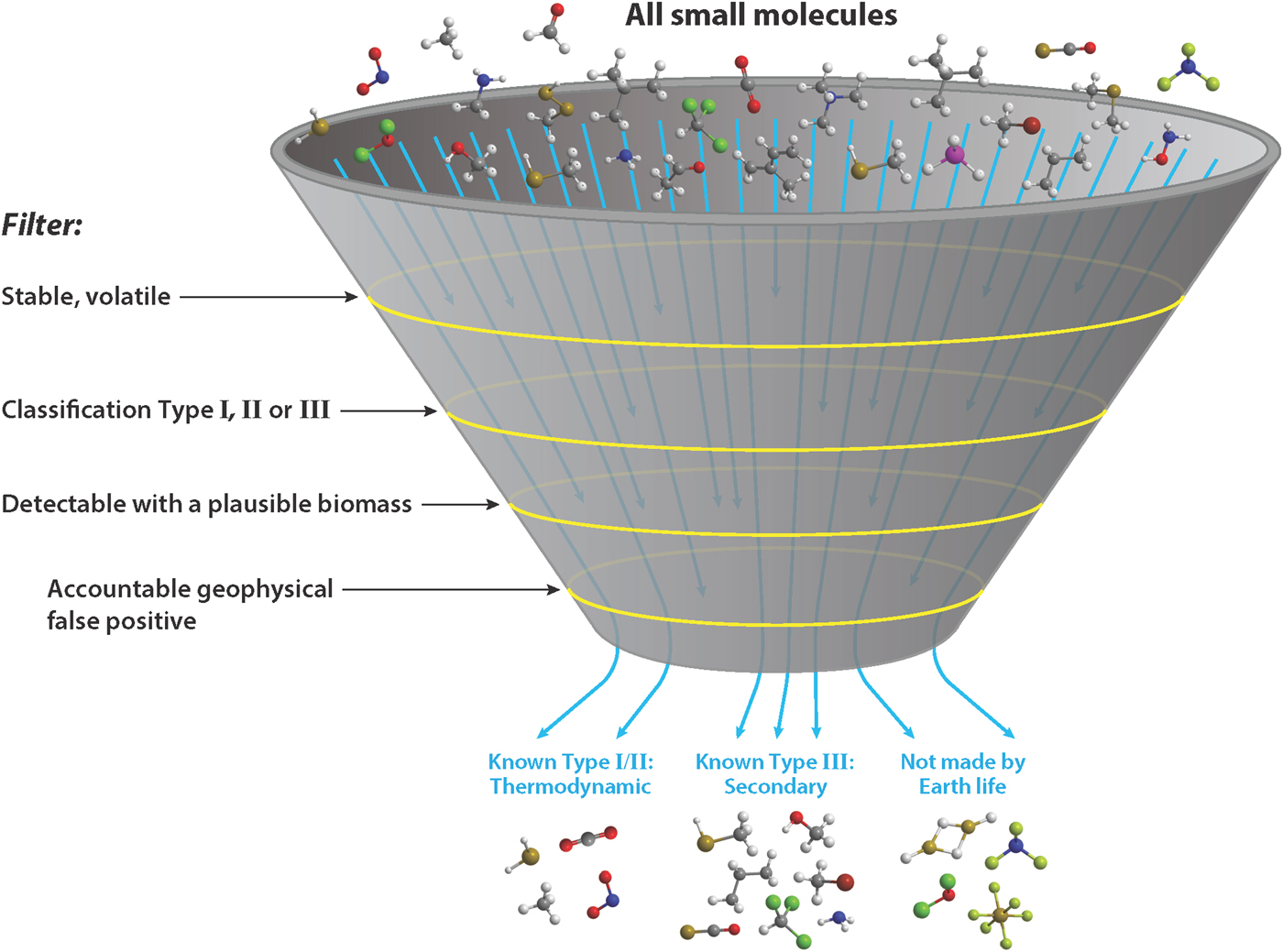
The all small molecule approach to biosignature gases will not be simple. We will adapt tools from ‘big data informatics’ to find the most efficient way to search through molecule properties in groups and classes before attempting detailed calculations on each molecule.
Our goal is for the community to use the list to study the chemicals that might be potential biosignature gases on exoplanets with atmospheres and surface environments different from Earth's. Applications of this approach to terrestrial biochemistry studies are also possible.
Outlook
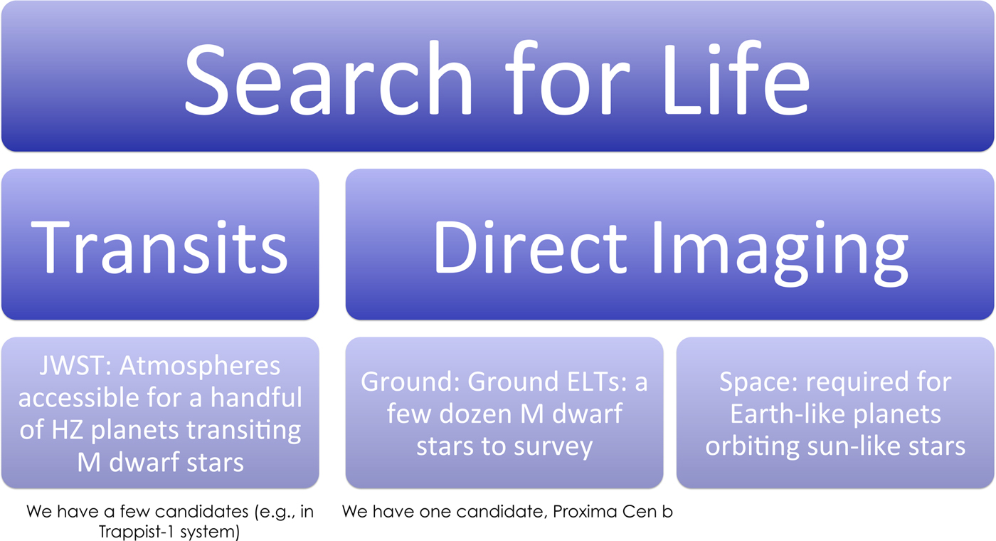
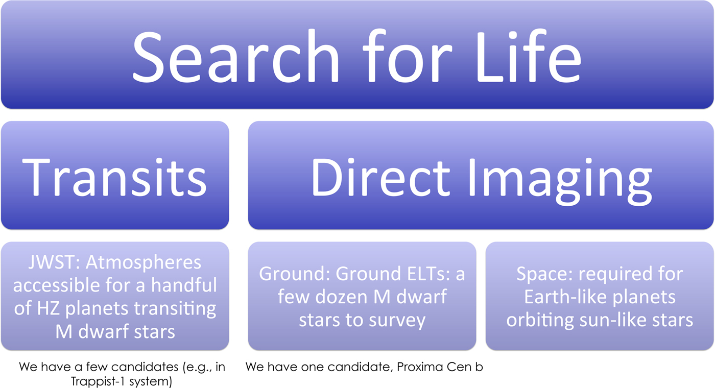
I presented a ‘Biosignature Drake Equation’ to outline the ingredients for a successful detection of biosignature gases. I gave three applications, one for the upcoming TESS/JWST combination where TESS and JWST are both scheduled to launch within 2 years of the writing of this paper. The second application is for the large (~30 m) ground-based telescopes now under construction, whose anticipated second generation instruments suitable for direct imaging of M dwarf star habitable-zone planets may be in place by the end of the 2020s. The third example is space-based direct imaging, required for detection and study of a number of Earth-like planets in the habitable zones of nearby sun-like stars. Here our first chance for a capable observatory is the Starshade Rendezvous Mission, still in a concept phase, but one growing in promise to launch in the middle or end of the WFIRST prime mission, which would be the late 2020s. The overall goal of the Biosignature Drake Equation is an illustrative estimate of how many planets with signs of life might be uncovered by each technique. See Fig. 3.
Schematic outlining the three dominant categories of observatories capable of the search for life by way of biosignature gases on exoplanets.
Despite an exuberant realization that the search for and detection of biosignature gases is within reach, the data may be of insufficient quality for more than a tentative detection. Additionally, even with high signal-to-noise high spectral resolution data, there may not be enough information about environmental context for a robust detection of life beyond Earth. It is more likely that a large pool of Earth-like planets with biosignature gases is likely to be required to establish with confidence that life exists beyond our Solar System.
To make sure all bases are covered, we proposed an ‘all small molecules approach’ to biosignature gas enumeration. While our list of ~14 000 molecules (described in Seager et al. Reference Seager, Bains and Petkowski2016) could take decades to complete detailed calculations of volatility, stability and spectral line lists for each molecule, we aim to spend 5–10 years on a coarser ‘triage’ type of approach. This approach will begin with examining and computing estimated properties and coarse spectral line calculations for classes of molecules or functional groups within molecules, in the context of hypothetical planet environments. From this approach we aim narrow down the list of molecules to focus more precisely on molecules that might actually be detectable with future space telescopes.
To conclude on a high note, two of the three observational approaches (see Fig. 3) described in this paper and for which the Biosignature Drake Equation was applied to, already have planets suitable for study by the next generation of telescopes. Typically each new class of exoplanet is just the tip of the iceberg, enabling us to embrace the possibility that habitable-zone planets and biosignature gases on them, may truly be out there amongst the nearest stars, just waiting to be found.
Acknowledgements
This work was originally submitted to the Templeton Foundation in August 2015 for their Exploring Exoplanets Symposium held at the Kavli Royal Society International Centre in Chicheley, UK, in September 2015. The concept of the ‘Biosignature Drake Equation’ was first presented at the Exoplanets in the Post-Kepler Era Symposium (https://www.cfa.harvard.edu/events/2013/postkepler/Exoplanets_in_the_Post_Kepler_Era/Main.html), held in Cambridge, MA, May 2013, in honour of Dave Latham's contributions to exoplanet science. The work in the section ‘Fraction of stars with planets’ is summarized from the author's contribution to the HDST report (Dalcanton et al. Reference Dalcanton2015). The work in the section ‘Spectroscopic gases produced by life’ is summarized from Seager & Bains (Reference Seager and Bains2015) and from Seager et al. (Reference Seager, Bains and Petkowski2016). I thank the organizers of the meeting, Sir Martin Rees, Paul Davies and Mary Ann, Meyers for an inspiring workshop. I thank the reviewer for useful comments that improved the paper.