1 Introduction
Surface roughness enhances the laminar-to-turbulent transition process in both low- and high-speed boundary layers. The transition process in boundary layers can be considerably altered using trips (roughness elements) by accelerating the transition region in both quiet and noisy environments (Tani & Sato Reference Tani and Sato1956; Klebanoff & Tidstrom Reference Klebanoff and Tidstrom1972). A multitude of numerical and experimental investigations have been carried out to understand trip-induced boundary-layer transition. However, the underlying physical mechanism, which is essential for high-speed vehicle design, remains insufficiently explained (Schneider Reference Schneider2008).
Past research suggests that different combinations of trip and flow configurations lead to different instability mechanisms. Acarlar & Smith (Reference Acarlar and Smith1987) and Klebanoff, Cleveland & Tidstrom (Reference Klebanoff, Cleveland and Tidstrom1992) studied hairpin vortices in a laminar boundary layer induced by a hemispherical roughness element. They suggested that these vortices, dominant in the transition mechanism, originate in the wake of the roughness element. Danehy et al. (Reference Danehy, Ivey, Inman, Bathel, Jones, Jiang, Webster, Lempert, Miller and Meyer2010) studied the size, shape and speed of flow structures in transitional hypersonic boundary-layer flows due to a cylindrical roughness element. Choudhari et al. (Reference Choudhari, Li, Wu, Chang, Edwards, Kegerise and King2010) suggested that a possible absolute instability in the upstream separation region was closely related to downstream unsteadiness. Using cylindrical roughness elements, they observed steady flow with
 $k/\unicode[STIX]{x1D6FF}$
(
 $k$
is the roughness height and
 $\unicode[STIX]{x1D6FF}$
is the untripped boundary-layer thickness at the trip location) less than 1 and unsteadiness with
 $k/\unicode[STIX]{x1D6FF}$
equal to 1.3 and 2.5. Redford, Sandham & Roberts (Reference Redford, Sandham and Roberts2010) studied the flow past a smoothly shaped roughness element at Mach 3 and 6 with free-stream acoustic forcing to ensure transition. They proposed a correlation for predicting transition induced by a three-dimensional roughness element at high speeds for roughness heights smaller than the boundary-layer thickness. Similarly, Tullio et al. (Reference Tullio, Parades, Sandham and Theofilis2013) studied a laminar–turbulent transition process induced by an isolated rectangular roughness element in a supersonic boundary layer at Mach 2.5 using direct numerical simulations (DNS). Their results indicate that the roughness element (
 $k/\unicode[STIX]{x1D6FF}=1$
) generates an unstable wake surrounded by a three-dimensional high-shear region. This wake can sustain rapid growth of instability modes. Unstable modes are related to the three-dimensional shear layer (varicose mode) or lateral shear layer (sinuous mode). The most unstable wake is observed to be the varicose type and grows much faster than the sinuous and boundary-layer modes. Iyer & Mahesh (Reference Iyer and Mahesh2013) performed DNS to study laminar to turbulent transition induced by a hemispherical roughness element (Danehy et al.
Reference Danehy, Bathel, Ivey, Inman and Jones2009). They found that roughness height and free-stream Mach number have a strong influence on transition.
Subbareddy, Bartkowicz & Candler (Reference Subbareddy, Bartkowicz and Candler2014) conducted DNS of an isolated cylindrical trip at Mach 6. We compare their findings with our data later in this paper, and therefore their work is discussed in detail. DNS is carried out at three different Reynolds numbers (
 $Re$
). We focus particularly on the high-Reynolds-number case in which transition to turbulence occurs just downstream of the trip. To understand the transition mechanism in the high-Reynolds-number case, the authors used dynamic mode decomposition (DMD) to identify dominant modes using snapshots of pressure. For detailed information on DMD, readers are referred to Schmid (Reference Schmid2010) and Rowley et al. (Reference Rowley, Mezic, Bagheri, Schlatter and Henningson2009). Three dominant DMD modes were studied. The first two modes (harmonic and subharmonic) were related to the horseshoe vortices, indicating that the dominant transition mechanism is due to the upstream vortex system. The third mode appeared to be associated with the shear layers, emanating from the top and sides of the trip, as the second dominant mode of transition. A large stand-off distance between the bow shock formed ahead of the trip and its stagnation region leads to the formation of highly unsteady upstream vortices in the high-
 $Re$
case. The upstream vortices then oscillate the bow shock via compression waves, producing periodic disturbances and causing breakdown. The oscillation of the bow shock is also influenced by pressure perturbations travelling upstream from the wake. Therefore, the unsteady shock system ahead of the trip is present in all three dominant modes. Recently, Duan & Xiao (Reference Duan and Xiao2017) studied the effects of roughness shape of isolated trips (cylinder, diamond, ramp at
 $k/\unicode[STIX]{x1D6FF}=1$
) on the transition mechanism of a Mach 6 transitional boundary layer using DNS. They found that a three-dimensional shear-layer instability leads to transition in all cases except in the cylindrical case where the horseshoe vortices are more dominant. The latter conclusion is consistent with Subbareddy et al. (Reference Subbareddy, Bartkowicz and Candler2014).
Let us now discuss prior studies of transitional hypersonic boundary layers due to an array of trips. Whitehead (Reference Whitehead1969) studied the flow field and drag characteristics of several trip shapes under laminar boundary-layer conditions at a free-stream Mach number of 6.8. Relevant to the current study, he presented the effects of trip spacing. The edge Mach number was 5.5,
 $k/\unicode[STIX]{x1D6FF}=2$
(
 $k=0.238$
cm). An array of spherical trips was mounted near the trailing edge of a 7.7
 $^{\circ }$
wedge. He observed that the trips appeared to act independently of the trip spacing, when
 $s/D$
(
 $s$
is the centre–centre trip spacing and
 $D$
is the spanwise trip width) is greater than 2. However, transition was delayed if the ratio of
 $s/D$
was equal to 2. This finding indicates that the smaller
 $s/D$
spacing leads to the delay of the transition onset and is less effective. A possible reason could be that this trip array acts more as a barrier than like individual vortex generators (Schneider Reference Schneider2008). However, the source of instability in any of these trip arrays was not discussed. Muppidi & Mahesh (Reference Muppidi and Mahesh2012) studied the transition mechanism of a Mach 2.9 supersonic flat-plate boundary layer due to distributed surface roughness. They observed that the interaction between a strong shear layer, generated over the roughness elements, and the counter-rotating pairs of streamwise vortices, formed underneath the shear layer, causes the shear layer to break down. Ergin & White (Reference Ergin and White2006) studied the flow fields around an array of cylindrical roughness elements near the critical Reynolds number under a subsonic flow configuration. They observed that locations of the maximum fluctuation intensity coincide with inflectional points in steady streamwise velocity profiles and suggest that a Kelvin–Helmholtz type instability leads to transition in their study.
Recently, Semper & Bowersox (Reference Semper and Bowersox2017) performed experiments, an extension of the work of Berry et al. (Reference Berry, Auslender, Dilley and Calleja2001), to quantify flow structures in a Mach 5.65 low-Reynolds-number (
 $Re_{\unicode[STIX]{x1D703}}=3600$
,
 $\unicode[STIX]{x1D703}=\text{momentum}$
thickness) boundary layer with a spanwise array of three-dimensional diamond-shaped trips with
 $s/D=2$
(blockage ratio = 50 %) and
 $k/\unicode[STIX]{x1D6FF}=1.48$
. They observed that a Kelvin–Helmholtz type instability could be a source of flow breakdown downstream. Following this experimental campaign, Shrestha & Candler (Reference Shrestha and Candler2016a
,Reference Shrestha and Candler
b
) and Shrestha et al. (Reference Shrestha, Nichols, Jovanović and Candler2017) performed DNS of the experiments to study their instability mechanisms. They obtained dominant frequencies that were associated with flow breakdown using power spectral density (PSD) and DMD. The instability mechanisms along with the effects of trip spacing and trip shape on these mechanisms under these particular flow and geometric configurations were not clearly identified.
Therefore, the present study aims to investigate the instability mechanisms of transitional hypersonic boundary layers due to an isolated diamond-shaped trip and an array of diamond-shaped trips (Semper & Bowersox Reference Semper and Bowersox2017) using DNS. First, we compare instability mechanisms between the isolated cylindrical trip (Subbareddy et al. Reference Subbareddy, Bartkowicz and Candler2014) and the isolated diamond-shaped trip. Second, we compare the mechanisms between the isolated diamond-shaped trip and the array of diamond-shaped trips. To build confidence in the simulations, we compare DNS data with the available experimental data. The paper is organized as follows: § 2 describes the basic equations and the numerical method; § 3 provides an overview of the experiment considered in the present investigation; § 4 illustrates the computational set-up; §§ 5 and 6 present the results of the simulations of both current trip configurations including DMD; and § 7 concludes the current study.
2 Basic equations and numerical method
We solve the unsteady compressible Navier–Stokes equations for calorically and thermally perfect air in conservative form:
 $$\begin{eqnarray}\frac{\unicode[STIX]{x2202}\boldsymbol{U}}{\unicode[STIX]{x2202}t}+\frac{\unicode[STIX]{x2202}\boldsymbol{F}_{j}}{\unicode[STIX]{x2202}x_{j}}=\frac{\unicode[STIX]{x2202}\boldsymbol{F}_{j}^{v}}{\unicode[STIX]{x2202}x_{j}},\end{eqnarray}$$
where the vector of conserved variables
 $\boldsymbol{U}$
is
 $$\begin{eqnarray}\boldsymbol{U}=\left[\begin{array}{@{}c@{}}\unicode[STIX]{x1D70C}\\ \unicode[STIX]{x1D70C}u_{i}\\ E\end{array}\right].\end{eqnarray}$$
The convective
 $\boldsymbol{F}_{j}$
and viscous
 $\boldsymbol{F}_{j}^{v}$
fluxes are
 $$\begin{eqnarray}\displaystyle & \displaystyle \boldsymbol{F}_{j}=\left[\begin{array}{@{}c@{}}\unicode[STIX]{x1D70C}u_{j}\\ \unicode[STIX]{x1D70C}u_{i}u_{j}+p\unicode[STIX]{x1D6FF}_{ij}\\ (E+p)u_{j}\end{array}\right], & \displaystyle\end{eqnarray}$$
 $$\begin{eqnarray}\displaystyle & \displaystyle \boldsymbol{F}_{j}^{v}=\left[\begin{array}{@{}c@{}}0\\ \unicode[STIX]{x1D70E}_{ij}\\ \unicode[STIX]{x1D70E}_{ij}u_{i}-q_{j}\end{array}\right],\quad (i,j=1,2,3). & \displaystyle\end{eqnarray}$$
In these equations,
 $u_{i}$
is the
 $i\text{th}$
component of velocity,
 $p$
is the pressure,
 $E=\unicode[STIX]{x1D70C}c_{v}T+(1/2)\unicode[STIX]{x1D70C}u_{i}u_{i}$
is the total energy,
 $T$
is the temperature,
 $c_{v}$
is the specific heat capacity at constant volume (
 $=0.718~\text{kJ}~\text{kg}^{-1}~\text{K}^{-1}$
) and
 $\unicode[STIX]{x1D70C}$
is the density. The viscous stress tensor
 $\unicode[STIX]{x1D70E}_{ij}$
and the heat flux vector
 $q_{j}$
are given by
 $\unicode[STIX]{x1D70E}_{ij}=2\unicode[STIX]{x1D707}\unicode[STIX]{x1D61A}_{ij}-(2/3)\unicode[STIX]{x1D707}\unicode[STIX]{x1D61A}_{kk}\unicode[STIX]{x1D6FF}_{ij}$
and
 $q_{j}=-k\unicode[STIX]{x2202}T/\unicode[STIX]{x2202}x_{j}$
, respectively, where
 $\unicode[STIX]{x1D61A}_{ij}$
is the symmetric part of the velocity gradient tensor, and
 $\unicode[STIX]{x1D6FF}_{ij}$
is the Kronecker delta. The ideal gas equation of state
 $p=\unicode[STIX]{x1D70C}RT$
is applied. Dynamic viscosity
 $\unicode[STIX]{x1D707}$
is calculated using Sutherland’s law,
 $\unicode[STIX]{x1D707}=aT^{1.5}/(T+b)$
with
 $a=1.458\times 10^{-6}$
Pa s, and
 $b=110.4$
K. The thermal conductivity
 $k=\unicode[STIX]{x1D707}c_{p}/P_{r}$
is computed using a constant Prandtl number
 $P_{r}=0.72$
and
 $c_{p}$
as the specific heat capacity at constant pressure (
 $=1.0~\text{kJ}~\text{kg}^{-1}~\text{K}^{-1}$
).
The present study utilizes an unstructured-grid finite-volume Navier–Stokes solver, US3D (Candler et al. Reference Candler, Johnson, Nompelis, Subbareddy, Drayna, Gidzak and Barnhardt2015), to simulate these flows. The solver has been extensively validated for numerous unsteady and compressible flow configurations, including compressible boundary layers and strong shock waves.
For the convective flux computation, we use a low-dissipation scheme based on the kinetic-energy consistent (KEC) method developed by Subbareddy & Candler (Reference Subbareddy and Candler2009). In this scheme, the inviscid flux is split into symmetric (non-dissipative) and upwind (dissipative) portions. The dissipative flux is pre-multiplied by a shock-detecting switch (Ducros et al. Reference Ducros, Ferrand, Nicoud, Weber, Darracq, Gacherieu and Poinsot1999), ensuring that the dissipation is active only at shocks. The sixth-order-accurate central KEC scheme is used for our present study, and the viscous fluxes are computed using second-order centred differences. Time integration is achieved using a second-order, implicit Euler method with point relaxation to maintain numerical stability and accuracy. The implicit system is solved with the full matrix data-parallel method (Wright, Candler & Prampolini Reference Wright, Candler and Prampolini1996).
3 ACE wind tunnel facility
Numerical simulations, consisting of the trip array, were performed in conjunction with an experimental campaign (Semper & Bowersox Reference Semper and Bowersox2017) carried out in the Actively Controlled Expansion (ACE) high-speed wind tunnel. This facility is a hypersonic blowdown wind tunnel located at the Texas A&M University. Uniform Mach numbers (to within 1 %) over a range of 5–7 are produced using a variable-Mach-number mechanism along with a range of
 $Re/m$
of
 $(0.7{-}7.0)\times 10^{6}~\text{m}^{-1}$
. The runtime of the facility is 40 s. The experiment is conducted on a 7.62 mm thick flat plate (508 mm long and 356 mm wide) with a 1.59 mm radius blunt leading edge. The leading edge of the model is positioned along the vertical centreline of the tunnel. The plate is aligned at an angle of attack of
 $-2^{\circ }$
to promote a favourable pressure gradient near its leading edge on the top surface. Trips are located at 95.2 mm (
 $x_{trip}$
) from the leading edge of the flat plate. Trip height (
 $k$
) is 4.76 mm and spanwise spacing between two trip centres (
 $s$
) is 6.36 mm (
 $s/D=2$
,
 $D=3.18$
mm is the spanwise trip width). Free-stream conditions are: Mach number (
 $M_{\infty }$
) is 5.92, stagnation temperature (
 $T_{o}$
) is 425 K, stagnation pressure (
 $P_{o}$
) is 448 kPa, and unit Reynolds number (
 $Re/m$
) is
 $4.6\times 10^{6}~\text{m}^{-1}$
. The post-shock Mach number (
 $M_{2}$
) is 5.65. For more details about the experimental facility and the campaign, the reader is referred to Semper & Bowersox (Reference Semper and Bowersox2017) and references therein.
4 Computational set-up
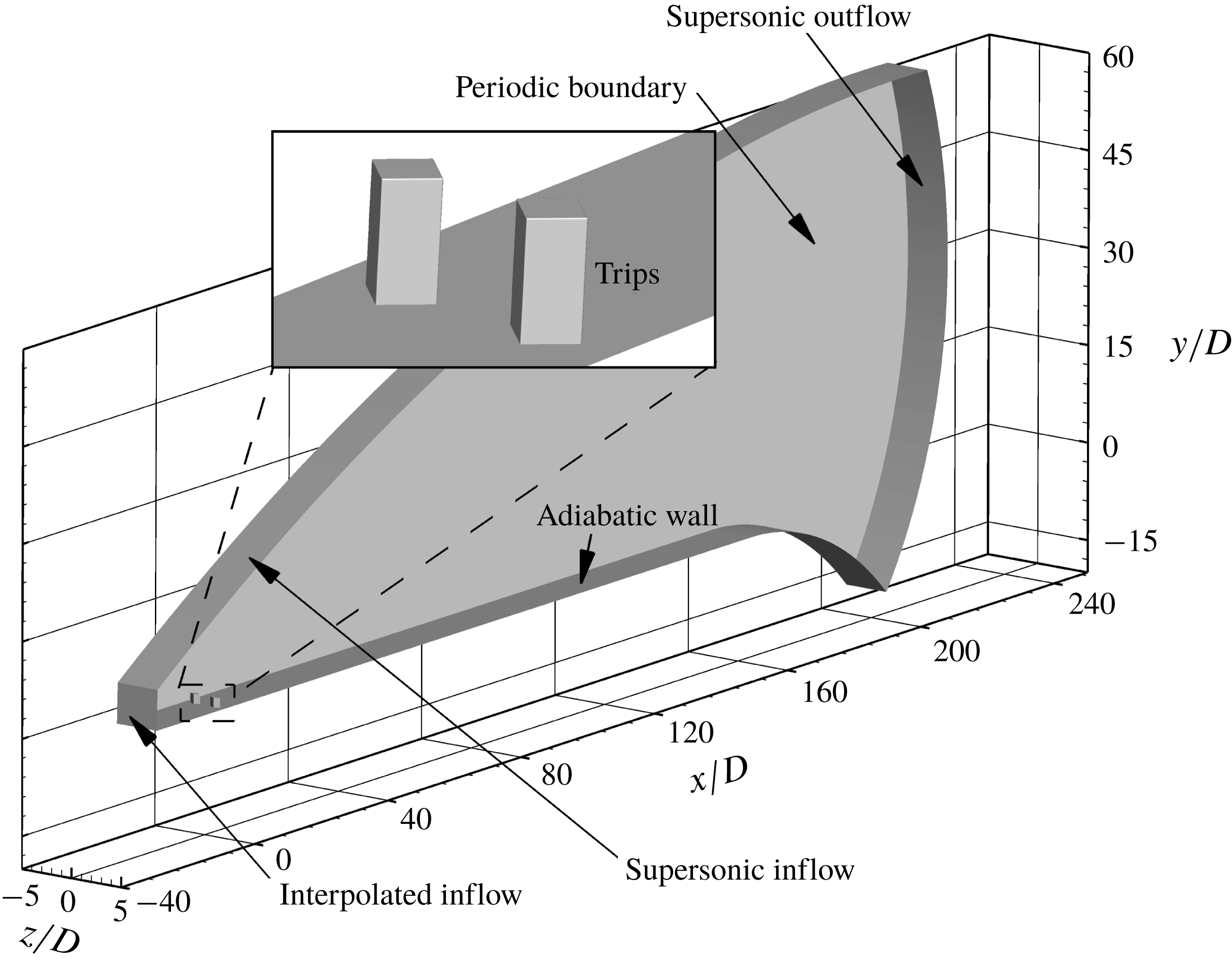
We model the flow in the ACE wind tunnel starting at the leading edge of the plate. For computational efficiency, we first perform a two-dimensional simulation over a flat plate that extends 70 mm from its leading edge. The boundary conditions of the two-dimensional domain are: the inflow is supersonic, the wall is adiabatic (the runtime of the facility is sufficient to equilibrate the wall temperature) and the outflow is supersonic. We extract wall-normal profiles of flow data at 30 mm (from the leading edge) of the two-dimensional domain. Second, we perform separate three-dimensional simulations using an isolated diamond-shaped trip and an array of diamond-shaped trips. We impose the extracted wall-normal profiles as the inflow boundary conditions of the three-dimensional simulations across the span. The streamwise location of the wall-profile extraction at 30 mm is selected to minimize effects of the upstream region of the trips on the inflow boundary of the three-dimensional simulations and maintain their computational efficiency. In the experiment, there are 47 trip elements. We use an array of two trips with periodic boundary conditions in the spanwise direction for computational efficiency. The use of the two trips also captures at least one spanwise harmonic mode and is closer to the experimental set-up than using only one trip. The three-dimensional domains of both trip configurations extend (streamwise) from 30 mm to 604 mm relative to the leading edge of the flat plate. Similar to the two-dimensional domain, the wall and the outflow boundary conditions are adiabatic and supersonic, respectively. A schematic of the boundary conditions for the three-dimensional domain of the trip array is shown in figure 1. The wall is curved at the end of the three-dimensional domain in order to minimize noise propagating upstream from the outflow boundary. The two trips are centred at
 $x/D=0$
,
 $z/D=-1$
and
 $x/D=0$
,
 $z/D=1$
. The spanwise extent of the domain with the isolated diamond-shaped trip is 20
 $D$
(
 $-10\leqslant z/D\leqslant 10$
). The isolated trip is centred at (
 $x/D=0$
,
 $z/D=0$
). In both three-dimensional domains, the upper edges of the trips are filleted with a radius of 10
 $\unicode[STIX]{x03BC}$
m to generate smooth grids near the edges. A constant time step (
 $\unicode[STIX]{x0394}t$
) of 20 ns is used in all the present simulations. We obtain a statistically converged solution after approximately 50 flow times (
 $X_{trip}/U_{\infty }$
) in both trip configurations.
A schematic of the boundary conditions of the three-dimensional domain using the trip array. Flow direction is left to right.

To validate our simulations, free-stream disturbances (
 $p_{rms}^{\prime }/P_{\infty }=1.5\,\%$
) are imposed in order to replicate the ambient experimental conditions. These disturbances may have a substantial effect on roughness-induced transition (Borg, Schneider & Juliano Reference Borg, Schneider and Juliano2008). Of the three possible disturbance modes (acoustic, entropy and vorticity), the acoustic mode, which originates from the turbulent boundary layer on the nozzle wall, is dominant (Laufer Reference Laufer2012). The free-stream disturbances are thus approximated as acoustic. We impose the disturbances as flow-parallel for simplicity. More information about the free-stream disturbances can be found in Semper & Bowersox (Reference Semper and Bowersox2017).
The pressure is assumed to have the following spectral form to satisfy the dispersion relation:
 $$\begin{eqnarray}\displaystyle & \displaystyle p^{\prime }(t)=\mathop{\sum }_{k=-N}^{k=N}p_{k}^{\prime }\text{e}^{\text{i}(\unicode[STIX]{x1D6FC}_{k}^{\pm })x-w_{k}t}, & \displaystyle\end{eqnarray}$$
 $$\begin{eqnarray}\displaystyle & \displaystyle \unicode[STIX]{x1D6FC}_{k}^{\pm }=\frac{w_{k}}{U_{0}\pm c_{o}}, & \displaystyle\end{eqnarray}$$
where
 $p^{\prime }$
is the time-dependent pressure fluctuation,
 $p_{k}^{\prime }$
is the complex frequency content of the
 $k$
th frequency,
 $\unicode[STIX]{x1D6FC}_{k}^{\pm }$
are the fast- and slow-moving wavenumbers,
 $w_{k}$
is the angular frequency,
 $x$
is the direction of the disturbance,
 $t$
is time,
 $U_{0}$
is the base free-stream velocity, and
 $c_{o}$
is the free-stream speed of sound. In our case, only fast-moving waves are considered as the inflow boundary condition of the two-dimensional domain is supersonic. Using the linearized Euler equations, we obtain the following relations:
 $$\begin{eqnarray}\left[\begin{array}{@{}c@{}}\unicode[STIX]{x1D70C}_{k}^{\prime }\\ u_{k}^{\prime }\\ T_{k}^{\prime }\end{array}\right]=\left[\begin{array}{@{}c@{}}{\displaystyle \frac{1}{\unicode[STIX]{x1D6FC}_{o}^{2}}}\\ -{\displaystyle \frac{\unicode[STIX]{x1D6FC}^{\pm }}{\unicode[STIX]{x1D70C}_{o}(\unicode[STIX]{x1D6FC}^{\pm }U_{o}-w_{k})}}\\ {\displaystyle \frac{(\unicode[STIX]{x1D6FE}-1)T_{o}}{\unicode[STIX]{x1D70C}_{o}c_{o}^{2}}}\end{array}\right]p_{k}^{\prime }.\end{eqnarray}$$
We can represent the pressure fluctuations in Fourier coefficients as
 $$\begin{eqnarray}\displaystyle & \displaystyle p^{\prime }(t)=\mathop{\sum }_{k=1}^{k=N}2|p_{k}^{\prime }|\cos (\unicode[STIX]{x1D6FC}_{k}^{\pm }x-w_{k}t+\unicode[STIX]{x1D719}_{p,k}), & \displaystyle\end{eqnarray}$$
 $$\begin{eqnarray}\displaystyle & \displaystyle |p_{k}^{\prime }|=\sqrt{\text{Re}(p_{k}^{\prime })^{2}+\text{Im}(p_{k}^{\prime })^{2}}, & \displaystyle\end{eqnarray}$$
 $$\begin{eqnarray}\displaystyle & \displaystyle \unicode[STIX]{x1D719}_{p,k}=\tan ^{-1}\left(\frac{\text{Im}(p_{k}^{\prime })}{\text{Re}(p_{k}^{\prime })}\right). & \displaystyle\end{eqnarray}$$
In the above equations,
 $|p_{k}^{\prime }|$
is the amplitude and
 $\unicode[STIX]{x1D719}_{p,k}$
is the phase of the
 $k$
th frequency component of pressure. Thus, the inflow profile is characterized using the pressure amplitude spectrum. Phase
 $\unicode[STIX]{x1D719}_{p,k}$
is random between 0 and 2
 $\unicode[STIX]{x03C0}$
to prevent superposition of peaks of different frequency modes. Furthermore, we filter the given PSD data from the facility using an interval of 2 kHz from 2 kHz to 250 kHz (the highest frequency captured in the experiment) to accurately resolve the frequencies of interest. Therefore, the
 $N$
that is stated in (4.4) is 125.
4.1 Grid convergence study
Unstructured grids are generated using LINK3D, a grid generator with a built-in parallel smoother. More information about LINK3D can be found in Drayna et al. (Reference Drayna, Haag, Bartkowicz and Gidzak2016). The unstructured grids contain hexahedral cells clustered into a large number of three-dimensional
 $i,j,k$
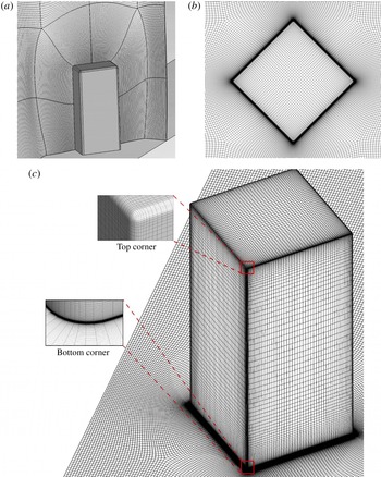
-ordered blocks. The grid generator allows a nested refinement of the block topology, which makes it possible to construct a high-resolution corridor around the roughness element. Away from this corridor, the grid is coarsened to keep the total grid size computationally efficient. Figure 2(a) shows the grid topology around a single diamond-shaped trip. Figures 2(b) and 2(c) show the grid in the vicinity of the trip from the top and the isometric views, respectively.
(a) Grid topology (the grid is refined in a corridor surrounding the diamond-shaped trip in order to resolve the flow physics while keeping the total grid size manageable), (b) top view of mesh, and (c) three-dimensional surface mesh around the trip.

Grid convergence studies are carried out for both trip configurations. As these studies are similar in both trip cases, we only present the convergence studies using the trip array. For a three-dimensional domain containing the trip array, we use a series of truncated domains to conduct a grid convergence study. The domains are truncated at
 $x/D=50$
. Consistent with Subbareddy et al. (Reference Subbareddy, Bartkowicz and Candler2014), the number of grid points diagonally spanning one of the diamond-shaped trips is used to conduct the grid convergence study. Spacings of 16 p.p.d. (points per diagonal) and 32 p.p.d. correspond to the truncated domains of 25 million and 50 million cells, respectively. The
 $y^{+}$
of the near-wall grid spacing for the two- and three-dimensional domains is 0.1. A sampling frequency (
 $f_{s}$
) of 5 MHz and the total sample number (
 $N$
) of 10 000 are used to compute time-averaged, root-mean-square (r.m.s.) and PSD (using the Hanning window given by Harris (Reference Harris1978)) of a flow quantity of interest in the present study. The PSD of pressure (for example) is computed as shown in (4.7), where
 $k$
ranges from 1 to
 $N_{f}$
discrete frequency disturbances and
 $\overline{p}$
is the mean pressure:
 $$\begin{eqnarray}\text{PSD}_{k}\;(\text{Hz}^{-1})=\frac{1}{2f_{s}}\left(\frac{|p_{k}^{\prime }|}{\overline{p}}\right)^{2}.\end{eqnarray}$$
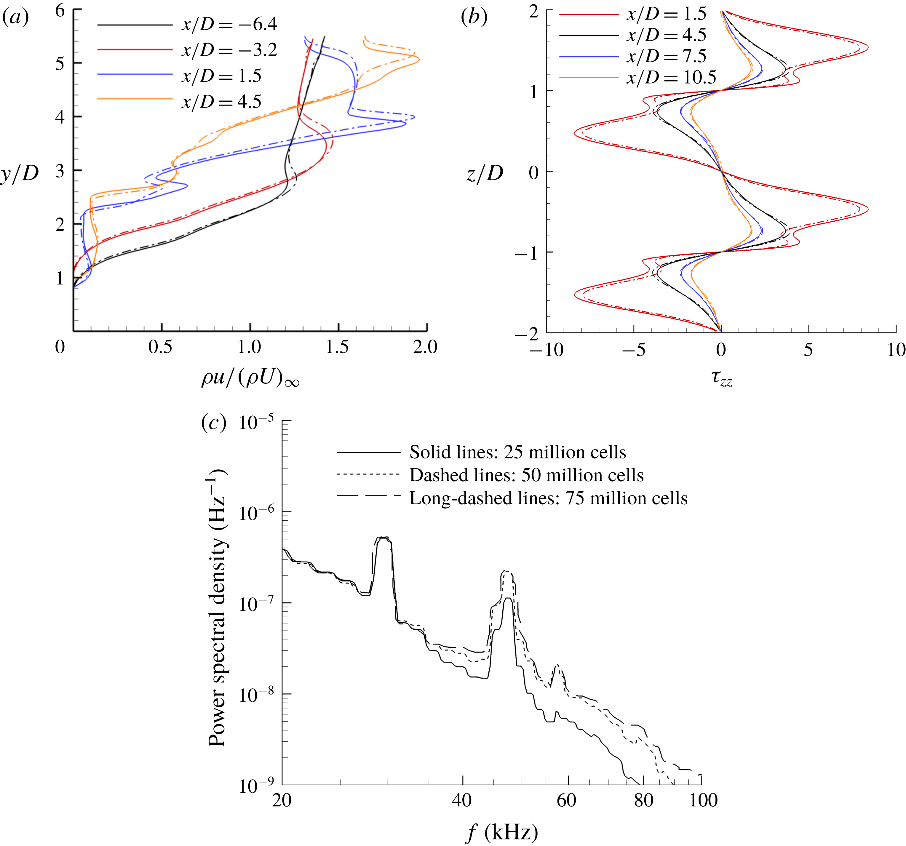
Grid convergence study of the three-dimensional domain consisting of the trip array using non-dimensionalized (a) mean streamwise mass flux in the wall-normal direction, (b) mean spanwise wall shear stress across span, and (c) PSD of pressure versus frequency at
 $x/D=26$
,
 $y/D=1.5$
and
 $z/D=1$
. Solid lines, 25 million cells (16 p.p.d.); dashed lines, 50 million cells (32 p.p.d.); and long-dashed lines, 75 million cells (48 p.p.d.).

Figure 3(a,b) shows grid convergence studies performed using time-averaged streamwise mass fluxes and spanwise wall shear stress in the two truncated domains. At all streamwise locations, the results agree well with each other. In figure 3(c), the PSD of pressure is plotted at
 $x/D=26$
,
 $y/D=1.5$
and
 $z/D=1$
in the two truncated domains. Local peaks at around 29 kHz and 45 kHz correspond to characteristic wind tunnel noise (Semper & Bowersox Reference Semper and Bowersox2017). However, the finer-grid domains (50 million and 75 million cells) more accurately capture a local peak at 58 kHz when compared with the experimental data at the same probe location in the next section. It will also be shown later that the local peak at 58 kHz is associated with a dominant mode of instability induced by the trip array. This finding indicates that the truncated domain with 50 million cells is grid converged, and accurately captures high-frequency coherent structures of interest. In the case of the isolated diamond-shaped trip, the three-dimensional domain with 90 million cells is also grid converged using the same time-averaged variables.
5 Comparison with experiment
In this section, the trip array DNS data are compared to the experiment using the wall-normal mean profiles of the streamwise mass flux, van Driest transformed velocity and Mach number. We also compare the PSD of pressure from the trip array DNS to the experiment. It is to be noted that the flow becomes turbulent at around
 $x/D=40$
(shown later), and frictional Reynolds number
 $(Re_{\unicode[STIX]{x1D70F}})=29$
based on the frictional velocity, the trip height and the kinematic viscosity at
 $x/D=86$
, where most of the comparisons are carried out.
The van Driest transformed mean velocity profile (van Driest Reference van Driest1956; van Driest & Blumer Reference van Driest and Blumer1962) is given by
 $$\begin{eqnarray}U_{vd}^{+}=\int _{0}^{U^{+}}\!\frac{\unicode[STIX]{x1D70C}}{\unicode[STIX]{x1D70C}_{w}}\,\text{d}U^{+}.\end{eqnarray}$$
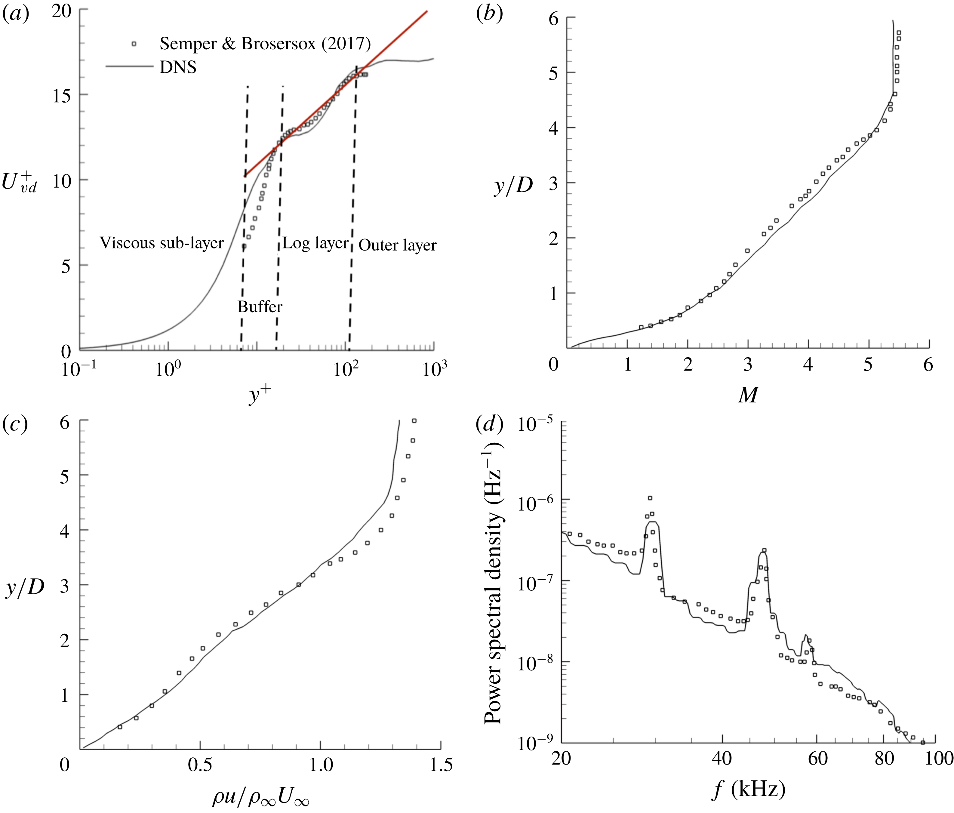
In figure 4(a), experimental and computed plots of the van Driest transformed mean velocity profiles are presented. In the buffer region, we observe good agreement for larger
 $y^{+}$
values, while in the log-law region, there is close agreement for all
 $y^{+}$
values. Possible reasons for a slight difference observed between our data and the experiment in the buffer region can be measurement issues or the use of only two trips instead of the 47 trips used in the experiment. In figure 4(b), the mean Mach number profiles from the DNS agrees fairly well with the experimental data.
Figure 4(c) presents a comparison of the mean streamwise mass flux (normalized by free-stream mass flux) with the experiment at
 $x/D=86$
on the symmetry plane (
 $z/D=1$
). We observe that there is close agreement between the numerical simulation and the experiment. PSD plots of pressure at (
 $x/D=26,y/D=1.4,z/D=1$
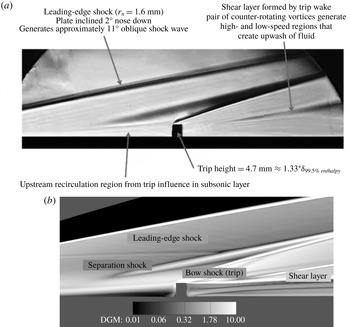
) are shown in figure 4(d). There is fair agreement between the experiment and the present study especially around peaks at 29 kHz, 45 kHz and 58 kHz. In figure 5, a Schlieren photograph of the experiment and an instantaneous density gradient magnitude (DGM) plot from the simulations are compared. The orientation of the upstream vortex system, the structure of the shock system and the shear layers observed in the experiment and the simulations agree well.
Wall-normal profiles of (a) van Driest transformed mean velocity, (b) mean Mach number, (c) mean streamwise mass flux at
 $x/D=86$
, and (d) PSD of pressure at
 $x/D=26$
and
 $y/D=1.4$
. All plots are at
 $z/D=1$
. Flow is fully turbulent at
 $x/D=86$
, where
 $x^{+}=7$
,
 $y^{+}=0.1$
and
 $z^{+}=0.7$
near the wall. At
 $x/D=26$
, flow is not turbulent.

We therefore have confidence in our simulations containing the trip array. We can extend this confidence to the isolated trip since both trip configurations share similar attributes regarding boundary conditions and meshing.
(a) Schlieren photograph from the experiment (Semper & Bowersox Reference Semper and Bowersox2017). (b) Density gradient magnitude contours from DNS at
 $z/D=1$
.

6 Results
We first investigate the isolated diamond-shaped trip and compare its instability mechanism with the isolated cylindrical trip (Subbareddy et al.
Reference Subbareddy, Bartkowicz and Candler2014). Later we study this mechanism in the case of the trip array and compare it with the isolated diamond-shaped trip. No free-stream disturbances are imposed so as to analyse the flow physics without free-stream noise. The free-stream values are used to non-dimensionalize their respective field variables. Particularly, frequency in hertz is non-dimensionalized to Strouhal number (
 $St$
), which is based on
 $U_{\infty }$
(free-stream velocity) and
 $D$
. The PSD of a flow quantity is normalized by its mean value.
6.1 Isolated diamond-shaped trip
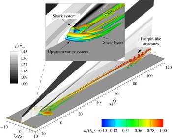
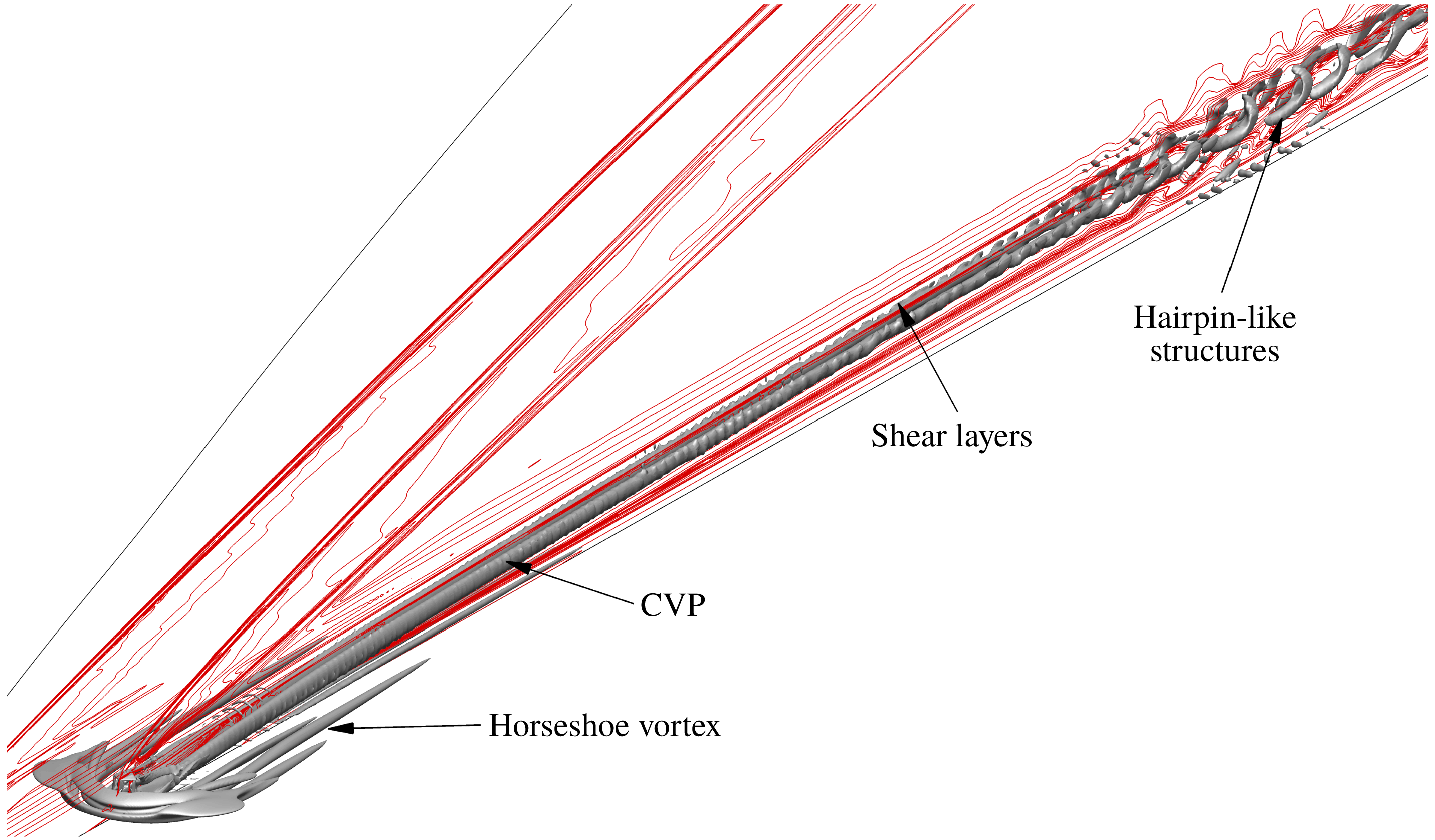
In this subsection, we characterize three distinct regions of unsteadiness in the isolated diamond-shaped trip flow field as shown in figure 6. The three regions are (1) the upstream vortex system, (2) the shock system ahead of the trip, and (3) the shear layers and the associated counter-rotating streamwise vortices that originate from its top, sides and downstream surfaces. The
 $Q$
-criterion (Hunt, Wray & Moin Reference Hunt, Wray and Moin1988) isosurfaces show the rotational motion of the upstream vortex system as well as the counter-rotating streamwise vortex pair (CVP) downstream. The
 $Q$
-criterion is the second invariant of the velocity gradient tensor, and is used to identify vortices:
 $$\begin{eqnarray}Q=-\frac{1}{2}\frac{\unicode[STIX]{x2202}u_{i}}{\unicode[STIX]{x2202}x_{j}}\frac{\unicode[STIX]{x2202}u_{j}}{\unicode[STIX]{x2202}x_{i}}.\end{eqnarray}$$
In figure 6, we observe streamwise fluctuations of isosurfaces of
 $Q$
-criterion downstream of the trip. These fluctuations later become hairpin-like structures, and eventually flow breakdown occurs. Next, we determine the source of these fluctuations and their critical frequencies, and compare with the isolated cylindrical trip.
 $Q$
-criterion (
 $=2.5\times 10^{8}$
) isosurfaces coloured by instantaneous streamwise velocity upstream and downstream of the isolated diamond-shaped trip. A symmetry plane is shaded by instantaneous pressure contours.

6.1.1 Upstream vortex system
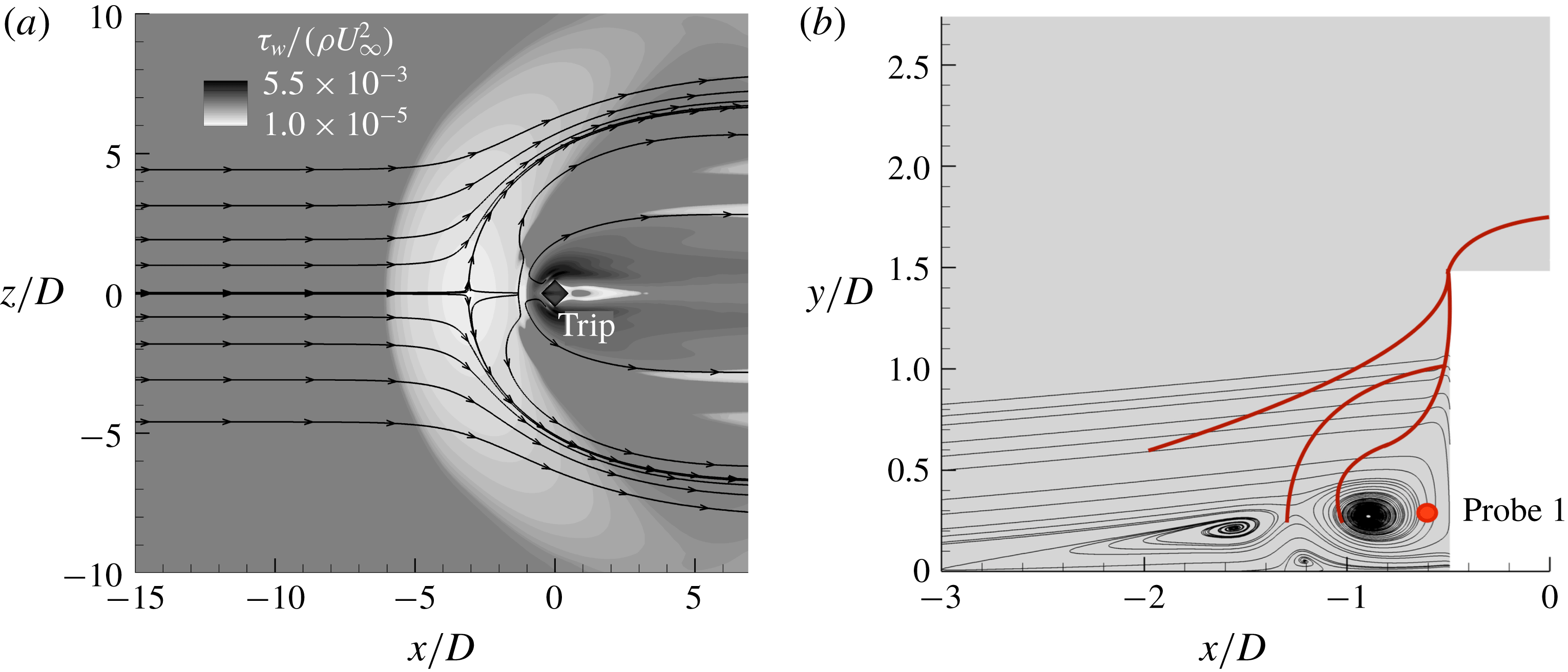
First, let us consider the upstream vortex system that forms in front of the trip. Figure 7(a) shows that the mean recirculation region extends approximately 3
 $D$
upstream of the trip. In the mean flow, there is a three-vortex system as shown in figure 7(b). Probe 1 (see figure 7
b) is located in the upstream vortex system to quantify unsteadiness and find peak-amplitude frequencies using the PSD (premultiplied by
 $St$
or
 $fD/U_{\infty }$
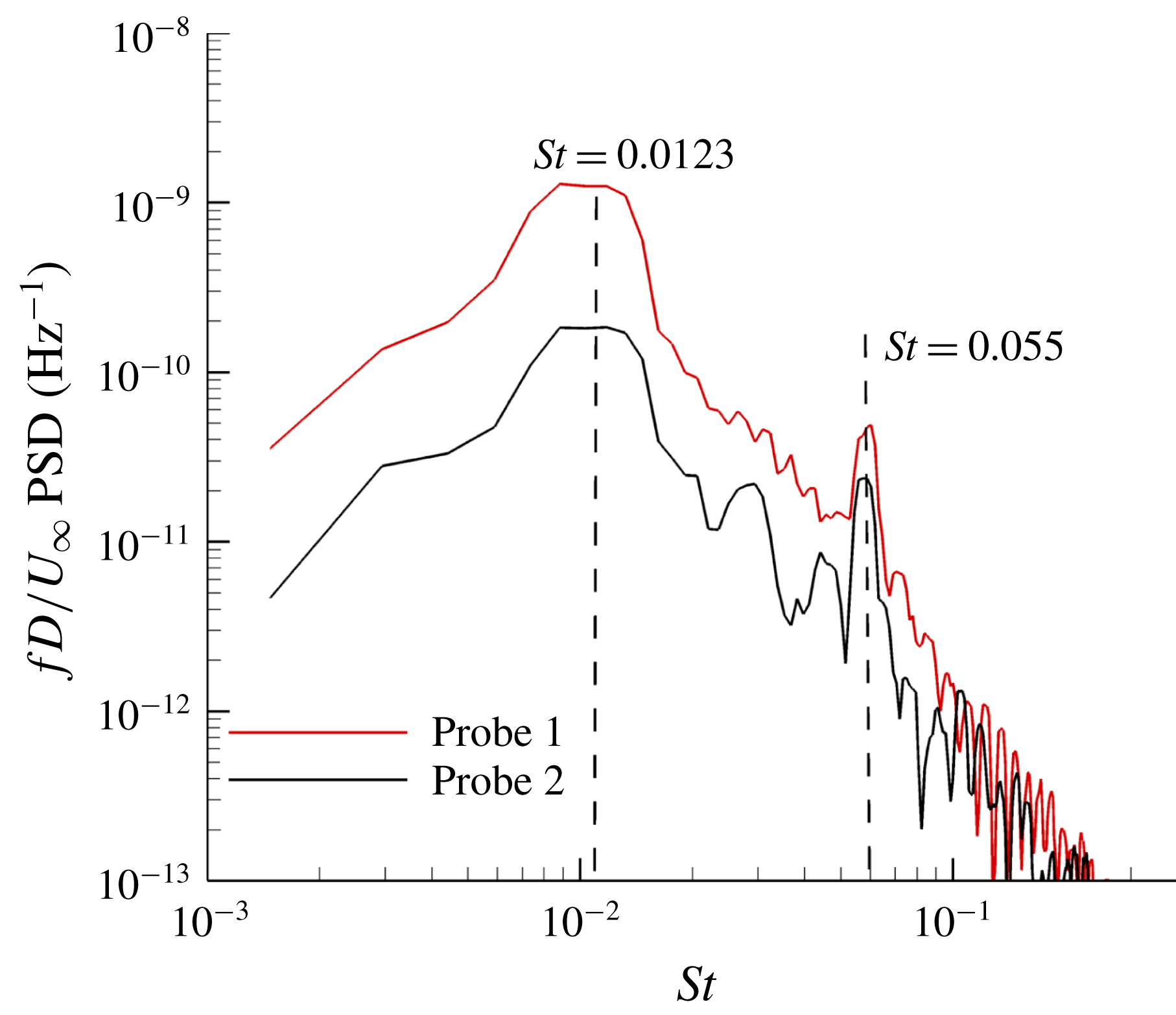
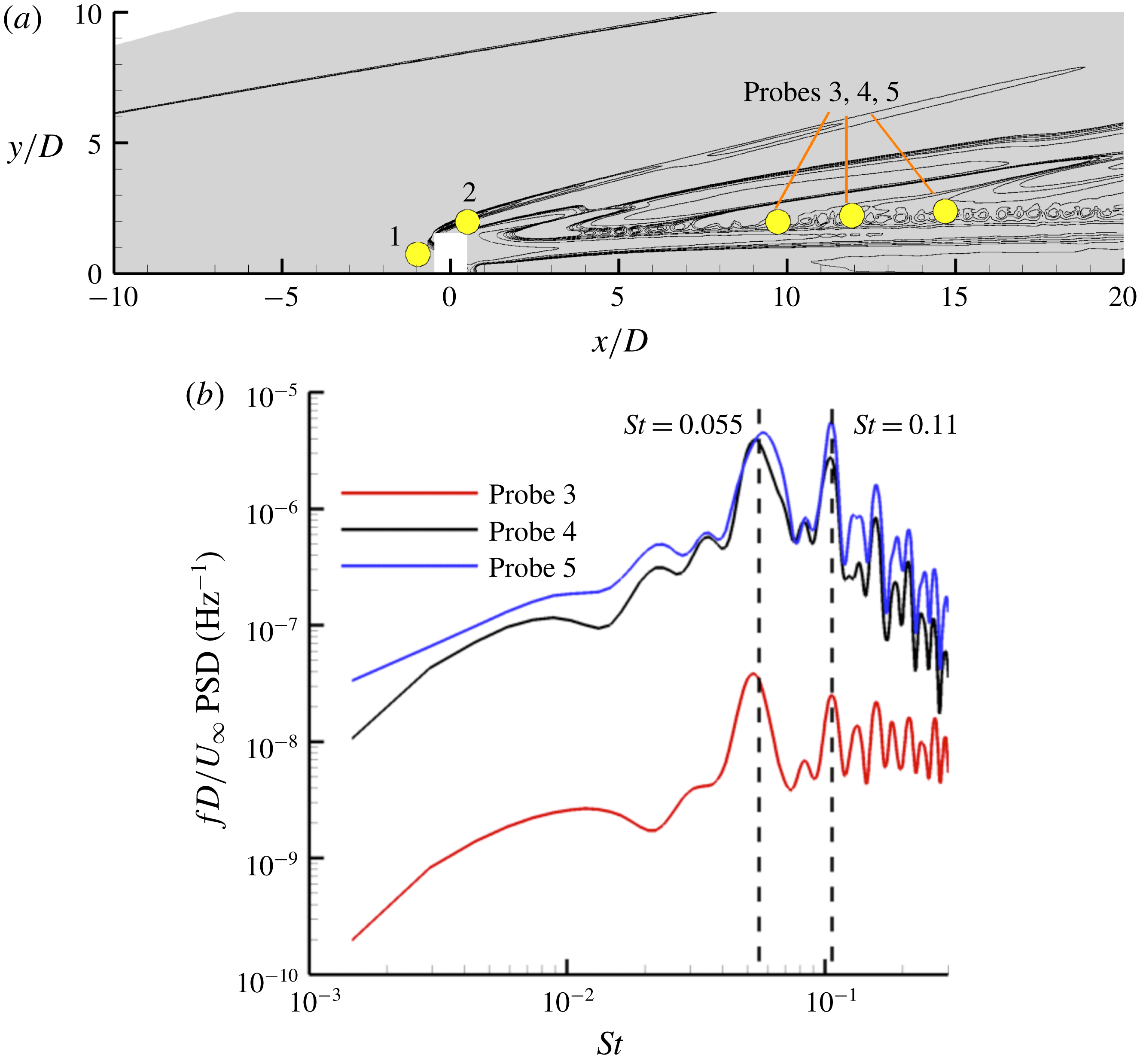
) of pressure fluctuations. In figure 8, the PSD indicates that the peak-amplitude frequency is at
 $St=0.0123$
(3 kHz) and shows a local peak frequency at
 $St=0.055$
(15 kHz). The low-frequency unsteadiness at
 $St=0.0123$
in the upstream vortex system is because the current simulation is at low Reynolds number (
 $Re_{k}=24\,000$
). Thus, this finding also agrees with the work of Baker (Reference Baker1979), in which low-Reynolds-number flow was found to have steady or low-frequency unsteady vortices in incompressible flows. The upstream vortices wrap the trip to form horseshoe vortices downstream.
(a) The mean streamwise wall shear contours around the trip (top view) and (b) the mean upstream recirculation region at
 $z/D=0$
using mean velocity stream traces. Red lines without arrows show the time-averaged shock system in this plane. A red dot indicates probe 1.

Premultiplied PSD of pressure at probes 1 and 2.

(a) R.m.s. of pressure and (b) the mean turbulent kinetic energy on the symmetry plane
 $z/D=0$
. Probe 2 (black dot) is located behind the bow shock.

6.1.2 Shock system
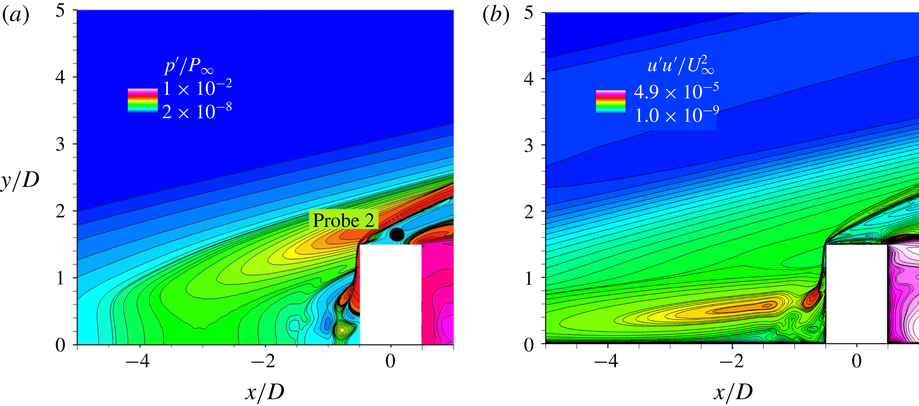
Second, we study the bow shock formed ahead of the trip as the top upstream portion of the trip is exposed to the supersonic flow. To understand the dynamics of the shock system, we plot the r.m.s. of pressure and the mean turbulent kinetic energy on the symmetry plane near the trip as shown in figure 9(a,b). In figure 9(a), we observe the high r.m.s. pressure at the bow shock, which indicates that the shock is unsteady. This observation is consistent with the mean turbulent kinetic energy contours as shown in figure 9(b). The unsteadiness of the bow shock is caused by the interaction between the bow shock and the upstream vortices via shocks (see figure 7
b). PSD analysis of pressure at probe 2 (see figure 9
a) behind the bow shock quantifies its unsteadiness in terms of frequency. As shown in figure 8, we observe the peak-amplitude frequency at
 $St=0.0123$
and a local peak frequency at
 $St=0.055$
. The high value of the r.m.s. of pressure in front of the shock on the top of the roughness element is most probably due to unsteadiness of the shock front performing essentially fore movements at Strouhal number 0.0123, and therefore this situation is usually characterized by a high skewness factor and a bimodal probability distribution of the pressure fluctuations. Thus, the shock system is unsteady, similar to the upstream vortex system. However, the dominant source of instability observed downstream of the trip is still unclear. Therefore, let us study downstream regions of the trip to obtain more insights into the instability mechanism.
(a) Probe locations are shown around the isolated trip on the symmetry plane. Contour lines are of instantaneous pressure. (b) Premultiplied PSD of pressure at probes 3, 4 and 5.

6.1.3 Shear layers/counter-rotating streamwise vortices
In this subsection, we study the unsteadiness downstream of the trip using PSD analysis of pressure at probes 3, 4 and 5 (figure 10
a). At these probe locations, the fluctuations of the
 $Q$
-criterion isosurfaces (figure 6) start to appear. In figure 10(b), we observe peak-amplitude frequencies at
 $St=0.055$
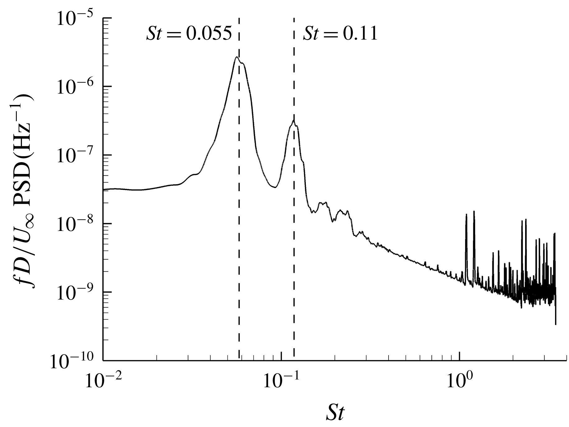
and 0.11 at all downstream probes. These critical frequencies can originate from the upstream vortex system, the unsteady shock system or the downstream region of the trip. Therefore, we perform a freezing operation – that is, we hold the flow state fixed during the simulation in a region of interest – and simulate the remainder of the flow domain for 10 flow times. In the present study, we freeze the upstream vortex system and the shock system (
 $x/D<0$
), and repeat the PSD analysis at the downstream probe locations. Thus, there is no unsteady forcing of the downstream flow by the upstream region. We still observe peak-amplitude frequencies at
 $St=0.055$
and 0.11 after the freezing operation as shown in figure 11. This finding indicates that the sources of unsteadiness observed downstream of the trip are the flow structures that originate from the downstream portion of the trip (
 $x/D>0$
). Because the upstream flow is frozen, it cannot cause the observed unsteadiness. Therefore, the local peak frequency at
 $St=0.055$
observed in the upstream vortex system and the shock system (see figure 8) is due to the pressure disturbances propagating upstream from the source through the subsonic region.
Premultiplied PSD of pressure at probe 4 after the freezing operation.

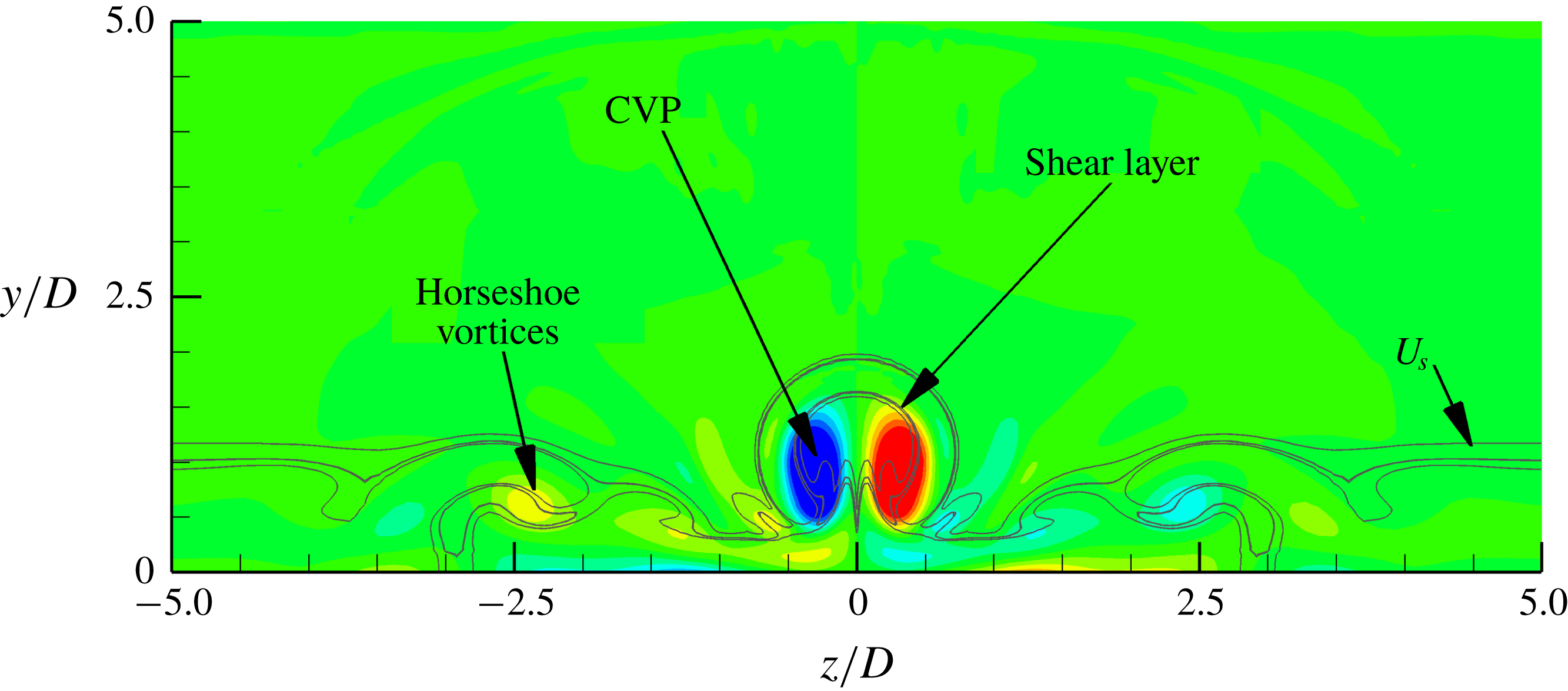
Figure 12 presents the flow structures downstream of the trip, such as the mean horseshoe vortices, the mean CVP and the mean shear layers on a streamwise plane at
 $x/D=10$
. The mean streamwise vorticity colours the streamwise plane. Contours of the mean streamwise vorticity show the CVP near the symmetry plane (
 $z/D=0$
) and the horseshoe vortices away from the symmetry plane. Contour lines on the plane indicate local shear values (
 $U_{s}$
) that represent the mean local shear layers:
 $$\begin{eqnarray}U_{s}=\sqrt{\left(\frac{\unicode[STIX]{x2202}u}{\unicode[STIX]{x2202}y}\right)^{2}+\left(\frac{\unicode[STIX]{x2202}u}{\unicode[STIX]{x2202}z}\right)^{2}}.\end{eqnarray}$$
We observe that the shear layers envelop the CVP and the horseshoe vortices downstream. The directions of each of the CVP vortices are upwash, as shown by the contours of mean streamwise vorticity. Therefore, the CVP lifts up away from the wall (Brandt Reference Brandt2014).
Contours of the mean streamwise vorticity showing the orientation of the mean CVP and the mean horseshoe vortices behind the isolated diamond-shaped trip at
 $x/D=10$
. The mean shear layers are shown using
 $U_{s}$
contour lines.

Shear layers (contour lines by
 $U_{s}$
to show local shear values) from the top of the trip interacting with the CVP (
 $Q$
-criterion isosurfaces coloured by streamwise velocity) on the symmetry plane. Both flow structures are instantaneous.

In figure 13, interactions between instantaneous shear layers (contour lines of local shear values on the symmetry plane) from the top edge and corners of the trip, and the instantaneous CVP (
 $Q$
-criterion isosurfaces) are shown. We observe that the shear layers, as well as the CVP, fluctuate spatially when they interact with each other downstream of the trip. The lift-up mechanism of the CVP amplifies the interaction. Owing to the interaction, the upper part of the CVP advects faster than its lower part. Thus, the CVP stretches streamwise to form hairpin-like structures. These structures, which get stretched further downstream, destabilize the shear layers. Therefore, the combined system of the shear layers and the CVP finally break down to turbulent flow. This finding indicates that the source of instability in the current trip configuration is a coupled system of the shear layers and the CVP.
6.1.4 Three-dimensional dynamic mode decomposition
Now let us find globally dominant modes using DMD and analyse their mode shapes. DMD is a post-processing technique that utilizes a number of snapshots from either experiments or simulations to extract a set of modes, each of which has a fixed oscillation frequency and decay/growth rate. A snapshot means a realization of a flow variable within a domain of consideration at a time instant. DMD extracts eigenvalues and eigenmodes using a linear mapping from the
 $n$
th snapshot to the
 $(n+1)$
th snapshot. Proper orthogonal decomposition (POD) is a similar method. POD extracts modes that have broadband frequency content, whereas each DMD mode has its own frequency. However, DMD modes are non-orthogonal, unlike POD modes. Therefore, this lack of orthogonality of DMD modes makes it challenging to systematically select a group of modes that is the strongest representation of the flow dynamics. Jovanović, Schmid & Nichols (Reference Jovanović, Schmid and Nichols2014) addressed this problem by developing a sparsity-promoting variant of the standard DMD algorithm. Sparsity-promoting dynamic mode decomposition (SPDMD) achieves a balance between the quality of approximation and the number of DMD modes. The adjustment is carried out using the least-squares deviation (between the matrix of snapshots and the linear combination of selected DMD modes) with a supplementary term that penalizes the
 $l_{1}$
-norm of the vector of DMD amplitudes. For more information on SPDMD, readers are referred to Boyd & Vandenberghe (Reference Boyd and Vandenberghe2004), Donoho (Reference Donoho2006), Candes, Wakin & Boyd (Reference Candes, Wakin and Boyd2008) and Jovanović et al. (Reference Jovanović, Schmid and Nichols2014).
In the present study, the snapshot domain is three-dimensional because a volumetric snapshot provides more detailed and accurate dynamics of the flow, which is complex. In DMD, snapshots of data are formed as columns into a matrix
 $\unicode[STIX]{x1D713}$
, of size
 $M\times N$
, say, where
 $M$
and
 $N$
are total degrees of freedom and number of snapshots, respectively. For the selection of the dominant modes, we use the Chu disturbance energy norm (Chu Reference Chu1965). For more information, readers are also referred to Hanifi, Schmid & Henningson (Reference Hanifi, Schmid and Henningson1996) and Nichols, Larsson & Bernardini (Reference Nichols, Larsson and Bernardini2017). In short, this norm
 $H$
(defined by (6.3)) utilizes the same sparsity processes as SPDMD but includes all the flow quantities:
 $$\begin{eqnarray}H=\int _{V}\left\{\frac{1}{2}\unicode[STIX]{x1D70C}_{o}(u^{\prime 2}+v^{\prime 2}+w^{\prime 2})+\frac{1}{2}\frac{c_{o}^{2}\unicode[STIX]{x1D70C}^{\prime 2}}{\unicode[STIX]{x1D6FE}\unicode[STIX]{x1D70C}_{o}}+\frac{1}{2}\frac{\unicode[STIX]{x1D70C}_{o}c_{v}T^{\prime 2}}{T_{o}}\right\}\text{d}V.\end{eqnarray}$$
In (6.3),
 $X_{o}$
and
 $X^{\prime }$
are the time-averaged and fluctuating values of flow variable
 $X$
, respectively. Mode shapes of pressure associated with the selected DMD modes are used so as to be consistent with the PSD analysis performed earlier.
The region of snapshot considered in the present trip configuration is in the range
 $x/D\in [-7,20]$
across the span height. The region was selected because (1) no flow breakdown region is included (minimizes nonlinearity), (2) all modes of transition can be studied, and (3) the number of degrees of freedom is smaller (compared to the entire domain). The sampling period is 5.0
 $\unicode[STIX]{x03BC}\text{s}$
, and the number of snapshots is 100 in the present study. Since the dominant frequencies observed in the previous PSD analysis are at
 $St=0.055$
and 0.11, and the present Nyquist frequency is at
 $St=0.37$
, the sampling frequency is sufficient to capture the relevant high-frequency modes. We use
 $M$
= 40 million cells and
 $N=100$
snapshots. Since the
 $\unicode[STIX]{x1D713}$
matrix is tall (
 $M$
) and skinny (
 $N$
), the TSQR algorithm (Sayadi & Schmid Reference Sayadi and Schmid2016) is implemented to carry out parallel QR factorizations. The algorithm is very efficient and scalable for the present case.
6.1.4.1 DMD results
We obtain two dominant DMD modes at
 $St=0.055$
and
 $St=0.11$
based on the Chu disturbance energy norm. The frequencies of these DMD modes are consistent with the previous PSD analysis. To quantify the contribution of each DMD mode to the flow dynamics, we calculate their respective performance loss. The performance loss due to a set of selected DMD modes is the deviation between the actual snapshot matrix
 $\unicode[STIX]{x1D713}$
and a reconstructed matrix formed by the linear combination of the selected DMD modes. Based on the performance loss, mode 1 (
 $St=0.055$
) and mode 2 (
 $St=0.11$
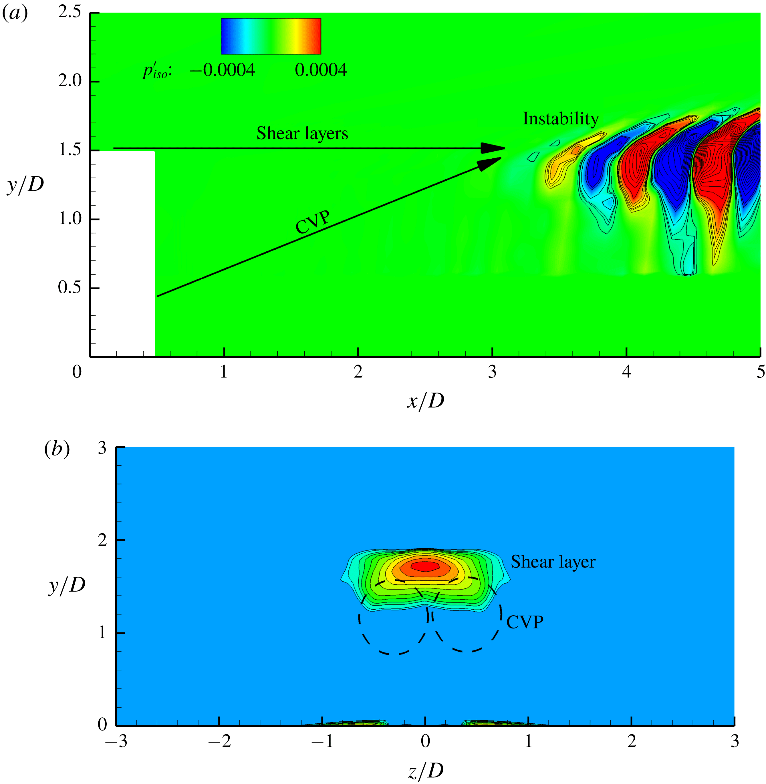
) contain approximately 27 % and 7 % of the total energy of the flow dynamics, respectively. In figure 14(a), pressure perturbations of mode 1 are plotted on the symmetry plane. Mode 2 has similar mode shapes, and therefore is not shown here. We observe that perturbations appear to originate from the downstream region of the trip. This finding is also consistent with the previous analysis, in which the sources of the unsteadiness are the shear layers and the CVP. Moreover, figure 14(b) indicates that mode 1 is a varicose-type instability in which the maximum interaction occurs between the wall-normal shear layers and the CVP.
Mode shapes of mode 1 (
 $St=0.055$
) on (a) the symmetry plane and (b) the streamwise plane (
 $x/D=10$
) using pressure contours.

6.1.5 Comparison to the isolated cylindrical trip
In this subsection, we compare the instability mechanisms of the isolated cylindrical and diamond-shaped trip flows. In the case of the isolated cylindrical trip, the source is the upstream vortex system, while that of the isolated diamond-shaped trip is a coupled system of the shear layers and the CVP from its downstream region. A reason behind this difference is the trip shape. Since the cylindrical trip is blunter compared to the diamond-shaped trip, the cylindrical trip has a larger stand-off distance between the bow shock and its stagnation point, and therefore additional upstream vortices. However, in the diamond-shaped trip, due to the sharper upstream trip surface, there are higher pressure gradients across its side edges, which lead to the formation of the shear layers being more unstable than the upstream vortex system. Hence, the downstream flow structures become the dominant source of instability in the isolated diamond-shaped trip. Furthermore, in the DMD analysis of the isolated diamond-shaped trip, we observe that the pressure perturbations are significantly more prominent in the downstream region than in the upstream vortex and the shock systems. However, in the isolated cylindrical trip, the dominant DMD modes show a strong presence of unsteadiness of the shock system that causes instabilities downstream. Therefore, the trip shape plays a significant role in the instability mechanism and flow unsteadiness around the trip.
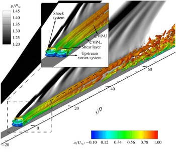
The
 $Q$
-criterion (
 $=2.5\times 10^{8}$
) isosurfaces coloured by the non-dimensionalized streamwise velocity upstream and downstream of the trip array. A spanwise plane on the left side shows instantaneous pressure contours.

6.2 Trip array
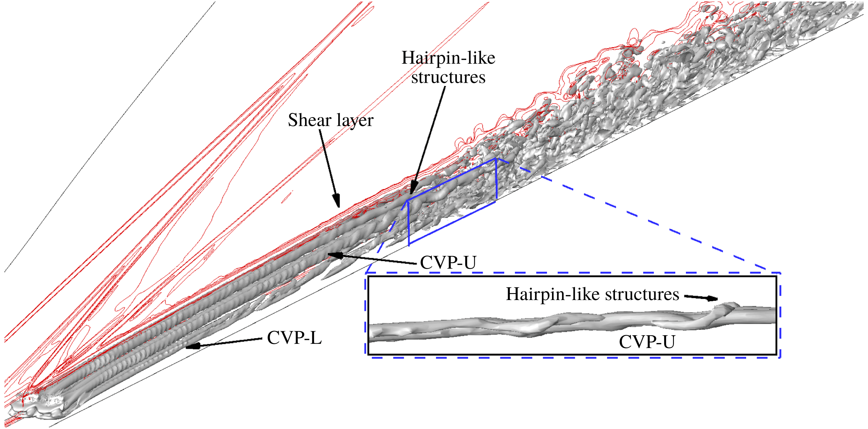
This subsection discusses and characterizes unsteadiness induced by the trip array as shown in figure 15. The
 $Q$
-criterion isosurfaces show the rotational motion of the two pairs of CVPs per trip. The two pairs of CVPs lie on top of each other, and therefore are named as CVP-L and CVP-U pairs (‘L’ for the lower pair near the wall, and ‘U’ for the upper pair away from the wall). These pairs (the CVP-L pair is formed due to wrapping of the upstream vortex system, and the CVP-U pair, similar to the CVP discussed earlier in the isolated diamond-shaped trip, originates from the wake of the trip) are clearly shown in figure 15. To understand the instability mechanism in the present trip configuration, we discuss flow structures in the region downstream of the trip array similar to the isolated diamond-shaped trip.
6.2.1 Shear layers/counter-rotating vortex system
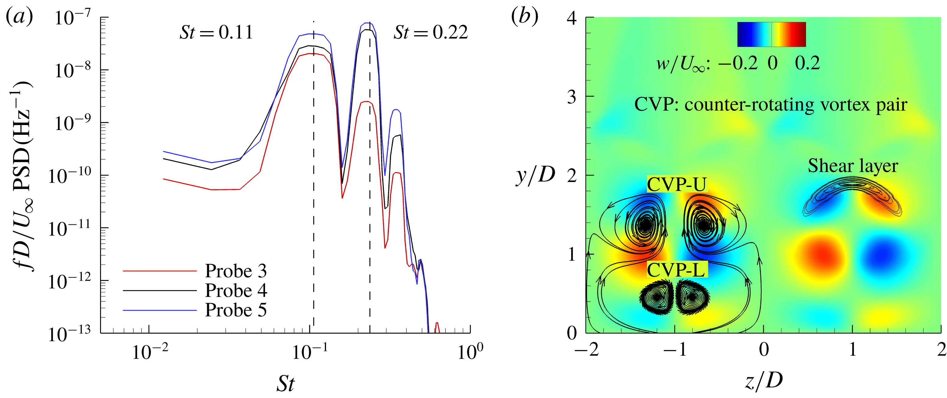
First, PSD analysis at probes 3, 4 and 5 is shown in figure 16(a). We observe peak-amplitude frequencies at
 $St=0.11$
, 0.22 and 0.33. To investigate the source of these peak-amplitude frequencies, we perform a freezing operation (similar to the isolated diamond-shaped trip) in the upstream vortex system and the shock system, and carry out PSD analysis at the downstream probes. We still observe the same peak-amplitude frequencies. This finding indicates that the source of these peak-amplitude frequencies is the region downstream of the trip array (consistent with the isolated diamond-shaped trip). Therefore, let us now study flow structures originating from the downstream region of the trip array to understand more about the instability mechanism.
(a) Pre-multiplied PSD of pressure at the downstream probes 3, 4 and 5. (b) Orientation of mean CVPs and mean three-dimensional shear layers surrounding the CVP at
 $x/D=10$
. Trip centres are at
 $z/D=-1$
and 1.

Figure 16(b) shows a detailed positioning of both mean CVP pairs along with the mean shear layers at
 $x/D=10$
. It is interesting to note that the mean CVP-L is closer to the symmetry plane in the trip array than the mean horseshoe vortices due to the isolated diamond-shaped trip. We observe that the CVP-U has upwash fluid movement, while the CVP-L has downwash fluid movement. Since the rotational motion of the CVP-U is greater than that of the CVP-L (see figure 15), the net fluid movement is away from the wall. Furthermore, the CVP-U is enveloped by the shear layers. This net upward movement of the CVP-U leads to more interaction between the shear layers and the CVP-U further downstream. Figure 17 shows that the interactions between the shear layers and the CVP-U lead to the formation of hairpin-like structures similar to the isolated diamond-shaped trip. These hairpin-like structures, which get further stretched due to the interactions, destabilize the shear layers. Finally, the hairpin-like structures and the shear layers break down to turbulent flow. Therefore, the source of instability remains a coupled system of the shear layers and the CVP-U.
Shear layers (contour lines by
 $U_{s}$
to show local shear values) from the top of the trips interacting with the CVP-U (
 $Q$
-criterion isosurfaces coloured by streamwise velocity) on the symmetry plane. Both flow structures are instantaneous.

6.2.2 Three-dimensional dynamic mode decomposition
Similar to the isolated diamond-shaped trip, let us now find the globally dominant frequencies, and study their mode shapes and overall contribution to the flow dynamics around the trip array using three-dimensional DMD and the Chu disturbance norm. The region of snapshot is in the range of
 $x/D\in [-20,20]$
across the span height. The sampling period is 5
 $\unicode[STIX]{x03BC}\text{s}$
, and the number of snapshots is 100. We use
 $M=40$
million cells and
 $N=100$
snapshots.
6.2.2.1 DMD results
We obtain two dominant DMD modes at
 $St=0.11$
(mode 1) and
 $St=0.22$
(mode 2) based on the Chu disturbance energy norm (shown by (6.3)). These DMD modes are consistent with the previous PSD analysis. To quantify the contribution of each DMD mode to flow dynamics, we calculate their respective performance loss. Based on performance loss, mode 1 and mode 2 carry 48 % and 15 % of the total energy of flow dynamics, respectively. Therefore, mode 1 is the dominant mode that causes instability downstream.
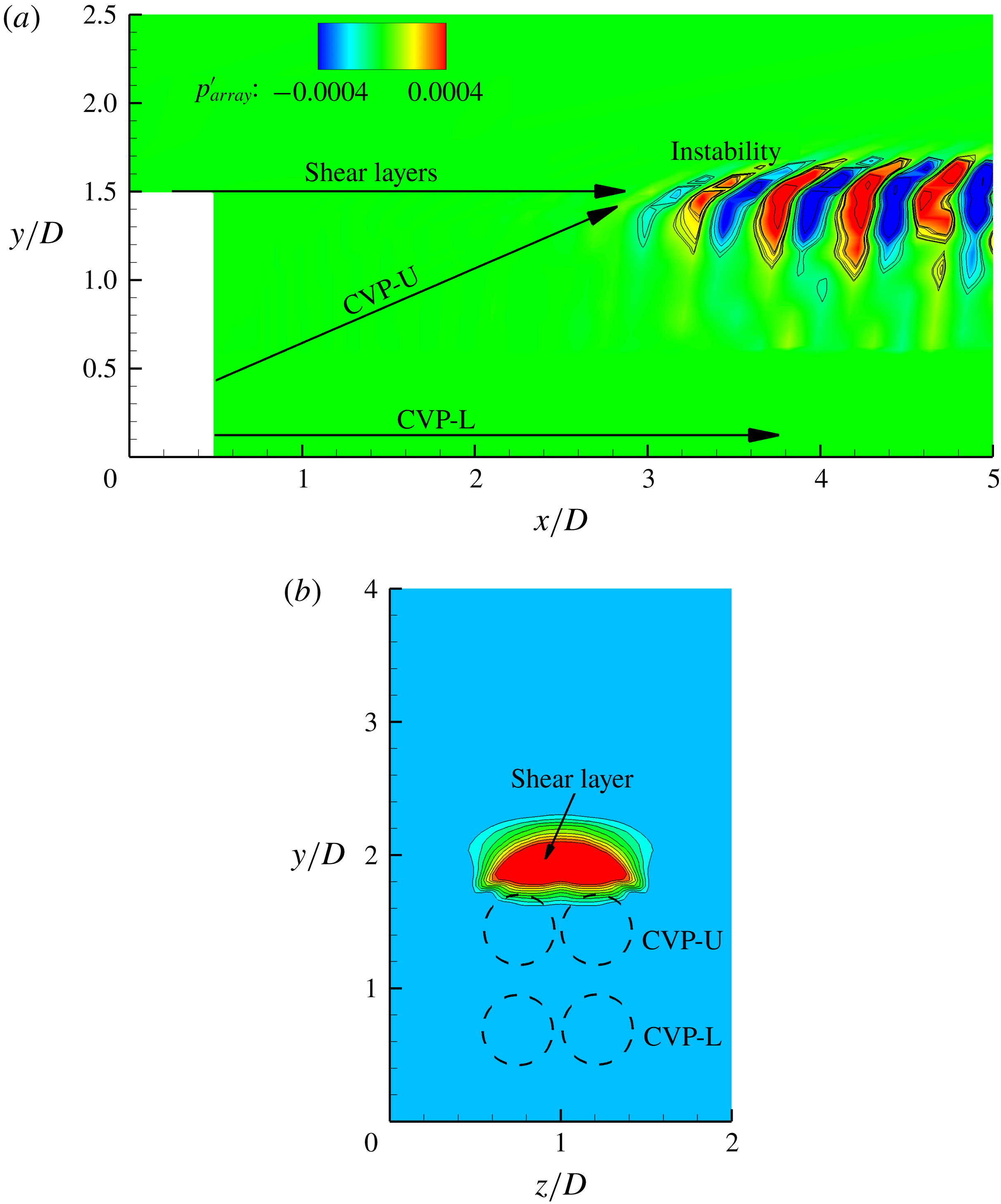
Let us now discuss mode shapes of mode 1 (mode 2 is similar) as shown in figure 18(a) on the symmetry plane (
 $z/D=1$
). We observe that the shear layers from the top sides of the trip and the CVP from its wake interact to cause instability downstream of the trip array. This finding indicates that the source of instability in the current trip configuration is similar to the isolated diamond-shaped trip. The dominant instability is consistently the varicose type as shown by figure 18(b). The PSD analysis carried out earlier agrees with the modal analysis.
Mode shapes of mode 1 (
 $St=0.11$
) on (a) the symmetry plane and (b) the streamwise plane (
 $x/D=10$
) using pressure contours.

6.2.3 Comparison to the isolated diamond-shaped trip
In this subsection, we compare the instability mechanisms of the isolated diamond-shaped trip and the trip array flows. The source of instability is observed to be consistent in both configurations and an intermediate case using
 $s/D=3$
by Shrestha & Candler (Reference Shrestha and Candler2018a
,Reference Shrestha and Candler
b
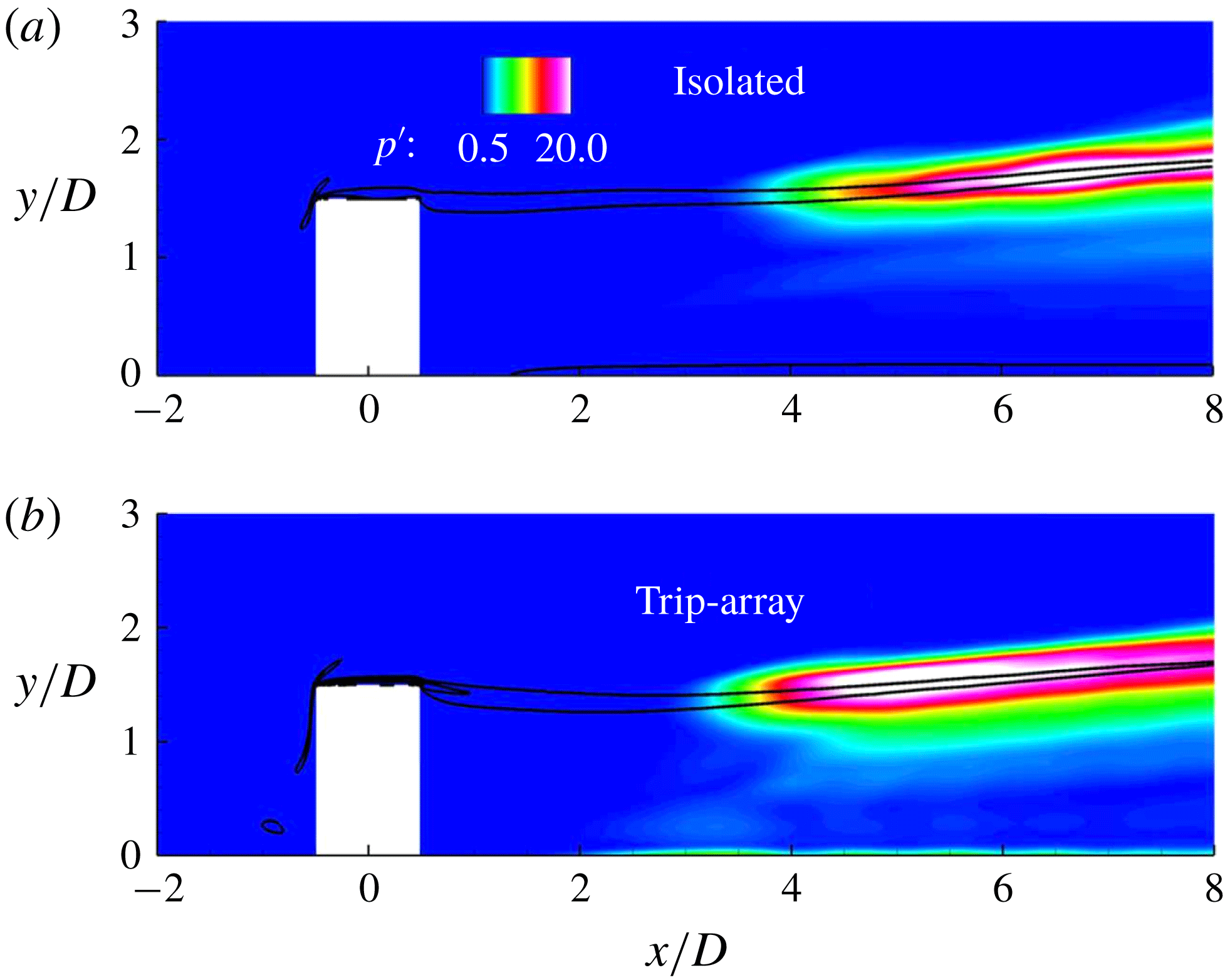
). Therefore, the trip spacing does not alter the source of instability. However, we found two differences regarding dominant frequencies (the most unstable mode) and instability onset locations. Instability onset location is the downstream location at which the shear layers and the CVP-U (the trip array) or the CVP (the isolated diamond-shaped trip) begin to interact with each other. The difference in the instability onset locations is around 1
 $D$
as shown in figure 19 using r.m.s. of pressure contours. This difference is small because the effect of neighbouring counter-rotating streamwise vortices from the wake of the trip array is minimal just downstream of the trips. However, the streamwise growth of instabilities in the trip array is higher than the isolated diamond-shaped trip as flow breaks down much earlier in the trip array. This finding is due to a combined effect of the CVP-U from the wake of neighbouring trips and the CVP-L from the upstream vortex system in the trip array. Dominant frequencies are at
 $St=0.055$
in the case of the isolated trip, and at
 $St=0.11$
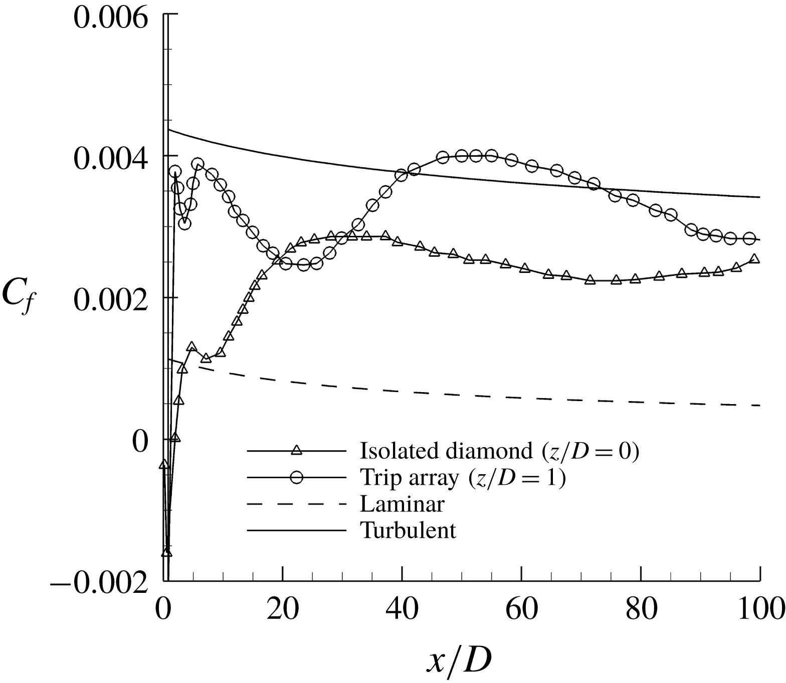
in the case of the trip array. This disparity in the dominant frequencies can be due to the difference in spanwise spacing available for the CVP (isolated diamond-shaped trip: more spacing and lower frequency) or the CVP-U (trip array: less spacing and higher frequency) as these downstream flow structures force the shear layers to become unstable. In figure 20, we observe that the flow becomes transitional earlier in the trip array configuration based on the streamwise evolution of the mean skin-friction coefficient (
 $C_{f}$
defined by (6.4)):
 $$\begin{eqnarray}C_{f}=\unicode[STIX]{x1D70F}_{wall}/(\unicode[STIX]{x1D70C}_{\infty }U_{\infty }^{2}).\end{eqnarray}$$
In (6.4),
 $\unicode[STIX]{x1D70F}_{w}$
is the mean wall-shear stress. This finding indicates that the trip array configuration is more effective in tripping the incoming laminar boundary layer, and therefore this tripping arrangement is used in high-speed vehicles like scramjets, where turbulent flows ahead of their engines are desirable.
Comparison of the instability onset locations in the isolated diamond-shaped trip and the trip array using r.m.s. of pressure at
 $z/D=1$
. Black contour lines indicate local shear values
 $U_{s}$
to show the mean shear layers from the top edges of the trip.

Comparison of the mean skin-friction coefficient along the streamwise direction in the isolated diamond and the trip array configurations.

7 Conclusion and future work
DNS are used to study laminar–turbulent transition of a hypersonic boundary layer due to an isolated diamond-shaped trip and a spanwise array of diamond-shaped trips. The current study is based on a low-Reynolds-number hypersonic flow experiment that was carried out at the Texas A&M University. The DNS results obtained agree with the experimental data. To investigate the instability mechanisms in both trip configurations, the flow is not perturbed by free-stream disturbances or any other forcing apart from the trip. Visualization of the flow shows three prominent regions of unsteadiness consistently observed in both trip configurations: (1) the upstream vortex system, (2) the shear layers/counter-rotating vortex system, and (3) the shock system. Analysis of the PSD and three-dimensional DMD of pressure indicates that the source of instability in both trip configurations is a coupled system of the shear layers from the top edges and corners of the trip, and the counter-rotating streamwise vortices from the wake. The interaction between the wall-normal shear layers (varicose mode) and the counter-rotating vortices leads to the formation of hairpin-like structures that eventually break down to turbulent flow. These findings contradict that of the isolated cylindrical trip where the upstream vortex system is the dominant mode of instability. Therefore, the trip shape plays a significant role in the source of instability, and the trip spacing does not alter the dominant mode of instability. However, the trip spacing changes the dominant frequencies of the instability and the instability onset locations. The peak-amplitude frequency associated with instability is higher in the trip array, while its instability onset location moves further upstream than the isolated diamond-shaped trip. Furthermore, flow breaks down earlier in the trip array. In both trip configurations, the peak-amplitude frequencies, which are observed downstream of the trips, also appear in the upstream vortex system and the shock system as pressure disturbances propagate upstream of the source of instability through the subsonic region.
A recent paper by Shrestha & Candler (Reference Shrestha and Candler2018b ) presents effects of free-stream Reynolds numbers and trip heights (similar to Williams & Smits (Reference Williams and Smits2017)). They found that the source of instability was consistent with the present finding over a selected range of free-stream Reynolds numbers and trip heights. Future work includes an investigation using different Mach numbers to enhance our understanding of the transition mechanism in a broader sense. Based on the effectiveness of the methodology used in the present study, DMD, PSD and DNS have been observed to be useful tools to study the instability mechanism.
Acknowledgement
The authors gratefully acknowledge the Office of Naval Research through grant number N00014-15-1-2522 for the support of this research. The suggestions and findings obtained herein are those of the authors and should not be interpreted as necessarily representing the official policies or endorsements, either expressed or implied, of the Office of Naval Research. The authors thank Drs M. T. Semper and R. D. W. Bowersox for providing experimental data to validate the present study, Mr J. Reinert for grid generation, and Drs I. Nompelis, J. W. Nichols and M. R. Jovanović for useful comments and suggestions.