1 Introduction
An unconstrained obstacle in a uniformly accelerated flow experiences an unbalanced hydrodynamic force on its surface which results in a continuous rotation of the obstacle. This phenomenon is sometimes called autorotation. As reviewed by Lugt (Reference Lugt1983), autorotation can be observed in the following situations: (i) autorotation perpendicular to the flow (e.g. rotating flat plate), (ii) autorotation parallel to the flow (e.g. lanchester propeller), (iii) autorotation due to shear flow and (iv) autorotation at arbitrary angle to the flow (e.g. spinning and rolling aircraft). Within these autorotation classifications, the present study numerically considers the flow-induced rotation of an S-shaped rotor, which consists of two half-circles assembled with zero overlap length, from a quiescent state. This situation relates to the above-mentioned autorotation case (i) and leads to a problem of a single degree of freedom (SDOF) with respect to the rotation angle.
Such an autorotation can be seen in, for example, vertical-axis wind turbines (VAWTs) having a rotor of the Savonius type. Jaohindy et al. (Reference Jaohindy, McTavish, Garde and Bastide2013, Reference Jaohindy, Ennamiri, Garde and Bastide2014) have studied computationally the autorotation of a Savonius wind turbine, adopting the built-in finite volume method with the commercially available computational fluid dynamics software package Star CCM+™. Their computations were carried out without a load, i.e. their computation does not include a brake such as a dynamo-electric generator and the torsional stress of a rotor shaft. They investigated the transient force on a Savonius rotor with respect to the aspect ratio. In contrast, much of the computational work for a Savonius rotor rotating with a predetermined constant angular velocity (i.e. non-autorotation) is available in, for example, Fujisawa (Reference Fujisawa1996) and Afungchui, Kamoun & Helali (Reference Afungchui, Kamoun and Helali2014) using a classical discrete vortex method, and Nasef et al. (Reference Nasef, El-Askary, AbdEL-hamid and Gad2013), Zhou & Rempfer (Reference Zhou and Rempfer2013), Shaheen, El-Sayed & Abdallah (Reference Shaheen, El-Sayed and Abdallah2015) and Tian et al. (Reference Tian, Song, VanZwieten and Pyakurel2015) using the computational fluid dynamics software package of either Ansys FLUENT™ or Star CCM+™ as reviewed by Roy & Saha (Reference Roy and Saha2013). Likewise, a few experimental studies on flow visualization around a Savonius rotor can be found in Fujisawa (Reference Fujisawa1992) using a wind tunnel and Nakajima, Iio & Ikeda (Reference Nakajima, Iio and Ikeda2008) using a water tunnel for a rotating rotor with a predetermined constant angular velocity, although many experimental studies have been restricted to the aerodynamic characteristics such as the torque and the power coefficients (see e.g. Ushiyama, Nagai & Shinoda Reference Ushiyama, Nagai and Shinoda1986). As mentioned, the flow-induced rotation of a rotor has been scarcely investigated. Therefore, this study selects an S-shaped rotor as a model system to study flow-induced rotation, and considers the mechanism of the S-shaped rotor automatically starting up from a quiescent state. Unlike all foregoing investigations of the flow-induced rotation, this paper sheds light on the scenario from the quiescent start to entering the limit cycle and the autonomous system in the present limit cycle which can account for the autorotation. Of course, for an actual VAWT, the influence of an external spring and damping plays an important role in the performance. However, the present study, as a preliminary step, neglects such an external influence and sheds light on the unsteadiness of the separated vortical flow from the tips of the rotor.
Among possible numerical approaches, one can use the finite element method, the boundary element method and the vortex method. The latter procedure was successfully implemented by Koumoutsakos & Leonard (Reference Koumoutsakos and Leonard1995) to compute the flow past an impulsively started circular cylinder and nicely verified against the asymptotic solution by Bar-Lev & Yang (Reference Bar-Lev and Yang1975). The present work basically follows the remeshed vortex particle method of Ploumhans & Winckelmans (Reference Ploumhans and Winckelmans2000) for the flow-induced rotation of an S-shaped rotor. This vortex particle method was nicely verified by Ueda, Kida & Iguchi (Reference Ueda, Kida and Iguchi2013) for a creeping flow about a two-cylinder cluster. The present vortex method does not require a boundary-fitted grid on a rigid obstacle and it is therefore suited for computing such a flow-induced rotation of a rotor, as mentioned above.
As shown in Nozu & Tamura (Reference Nozu and Tamura1997) for the flow past a square prism at larger than
 $Re=1000$
, vortex shedding from a two-dimensional obstacle produces fine-scale three-dimensional vortices. Three-dimensionality in a wake behind a circular cylinder is known to be observed at larger than
 $Re\approx 200$
(see Williamson Reference Williamson1996), and the transverse enstrophy computationally appears to saturate at about
 $t=150$
after the impulsive movement at
 $Re=300$
(see Cottet & Poncet Reference Cottet and Poncet2003). The present benchmark flow at
 $Re=500$
is thus found to almost behave like a two-dimensional shedding mode and it is compared with previous two-dimensional computational results. Furthermore, Tian et al. (Reference Tian, Song, VanZwieten and Pyakurel2015) showed that two-dimensional computation can give acceptable results for a Savonius rotor.
The paper is organized as follows. Section 2 states the problem addressed and the numerical methodology. The pressure distribution on the rotor surface which causes the torque on the rotor can be calculated by solving the boundary integral equation with respect to Bernoulli’s function, and it is nicely verified for a circular cylinder without and with rotating motion against previous computational and analytical results in § 3.1. The flow-induced rotation of the S-shaped rotor is then computed in § 3.3. In this computation, the S-shaped rotors having various values of the moment of inertia (MOI) start to rotate automatically from a quiescent state. In § 3.2, the scenario of the S-shaped rotor automatically starting up from a quiescent state and entering the limit cycle is elucidated. In § 3.3.1, results for the hydrodynamic characteristics and the flow patterns around the rotor are given. In § 3.3.2, after the rotor reaches a stable rotation, the flow-induced rotation of the rotor is explained from the viewpoint of an autonomous system, i.e. the limit cycle that is the trajectory of the rotor stably rotating is discussed within the framework of the Poincaré–Bendixon theorem mentioned in appendix C. Finally, we summarize the results obtained in the paper.
2 Numerical procedure
This section addresses the employed remeshed vortex particle method together with the boundary integral equation with respect to Bernoulli’s function to calculate the pressure on the rotor surface. It also benchmarks this numerical procedure against earlier numerical and analytical results for a circular cylinder abruptly made to rotate and translate in § 3.1.
2.1 Problem statement and governing equations
We consider the unsteady incompressible viscous flow about a body,
 ${\mathcal{C}}_{b}$
(see figure 1). The body has centre
 $\boldsymbol{O}$
, boundary
 $\unicode[STIX]{x2202}{\mathcal{C}}_{b}$
and diameter
 $D$
. At
 $t\rightarrow +0$
, a constant flow
 $V\boldsymbol{e}_{x}$
with
 $V>0$
impulsively approaches the body. At the same time, the body rotates with angular velocity
 $\unicode[STIX]{x1D6FA}(t)\boldsymbol{e}_{z}$
in the counterclockwise direction. The time
 $t_{0}$
is non-dimensionalized based on
 $D$
as
 $t:=2Vt_{0}/D$
. The fluid has kinematic viscosity
 $\unicode[STIX]{x1D708}$
. The resulting flow with typical Reynolds number
 $Re=VD/\unicode[STIX]{x1D708}$
has velocity and vorticity fields
 $\boldsymbol{u}(\boldsymbol{x},t)$
and
 $\unicode[STIX]{x1D714}(\boldsymbol{x},t)\boldsymbol{e}_{z}$
such that
 $\boldsymbol{u}(\boldsymbol{x},0)=\mathbf{0}$
and, for
 $t>0$
,
 $$\begin{eqnarray}\frac{\unicode[STIX]{x2202}\unicode[STIX]{x1D714}}{\unicode[STIX]{x2202}t}+\boldsymbol{u}\boldsymbol{\cdot }\unicode[STIX]{x1D735}\unicode[STIX]{x1D714}=\unicode[STIX]{x1D708}\unicode[STIX]{x1D6FB}^{2}\unicode[STIX]{x1D714}\quad \text{in }{\mathcal{D}},\end{eqnarray}$$
 $$\begin{eqnarray}\unicode[STIX]{x1D735}\boldsymbol{\cdot }\boldsymbol{u}=0\quad \text{and}\quad \unicode[STIX]{x1D714}=(\unicode[STIX]{x1D735}\wedge \boldsymbol{u})\boldsymbol{\cdot }\boldsymbol{e}_{z}\quad \text{in }{\mathcal{D}},\end{eqnarray}$$
with the no-slip boundary condition
 $$\begin{eqnarray}\boldsymbol{u}(\boldsymbol{x},t)=\boldsymbol{V}_{B}\quad \text{on }\unicode[STIX]{x2202}{\mathcal{C}}_{b}\end{eqnarray}$$
and far-field conditions
 $$\begin{eqnarray}\boldsymbol{u}(\boldsymbol{x},t)\rightarrow H(t)V\boldsymbol{e}_{x}\quad \text{and}\quad \oint _{{\mathcal{C}}_{r}}\boldsymbol{u}\boldsymbol{\cdot }\text{d}\boldsymbol{\ell }\rightarrow 0\quad \text{as }|\boldsymbol{x}|\rightarrow \infty ,\end{eqnarray}$$
where
 ${\mathcal{D}}$
denotes the dimensionless fluid domain,
 $\boldsymbol{V}_{B}$
is the unsteady velocity due to the rotation of the body
 ${\mathcal{C}}_{b}$
,
 $H$
denotes the usual Heaviside step pseudo-function (
 $H(t)=1$
for
 $t>0$
and
 $H(t)=0$
otherwise) and
 ${\mathcal{C}}_{r}=\{\boldsymbol{x}\mid |\boldsymbol{x}|=r\}$
.
A rotating obstacle
 ${\mathcal{C}}_{b}$
with angular velocity
 $\unicode[STIX]{x1D6FA}(t)\boldsymbol{e}_{z}$
immersed in a constant flow
 $V\boldsymbol{e}_{x}$
with
 $\boldsymbol{e}_{z}=\boldsymbol{e}_{x}\wedge \boldsymbol{e}_{y}$
.

2.2 Advocated vortex particle method
Using the Lagrangian formulation, the vorticity transport equation (2.1) is split into the Euler equation and the viscous diffusion equation:
 $$\begin{eqnarray}\frac{\text{d}\boldsymbol{x}}{\text{d}t}=\boldsymbol{u}(\boldsymbol{x},t),\quad \frac{\text{d}\unicode[STIX]{x1D714}}{\text{d}t}=\unicode[STIX]{x1D708}\unicode[STIX]{x1D6FB}^{2}\unicode[STIX]{x1D714}.\end{eqnarray}$$
The convective and diffusion steps are separately handled by a panel method and the particle strength exchange (PSE) method (see Degond & Mas-Gallic Reference Degond and Mas-Gallic1989).
The vortex method is based on the spatial discretization of the vorticity field which consists of Lagrangian particles. The discretized vorticity field can be written in the numerical quadrature, which is represented by vortex particles as
 $$\begin{eqnarray}\unicode[STIX]{x1D714}(\boldsymbol{x},t)=\mathop{\sum }_{i=1}^{N}\unicode[STIX]{x1D6E4}_{i}(t)\unicode[STIX]{x1D701}_{\unicode[STIX]{x1D716}}(\boldsymbol{x}-\boldsymbol{x}_{i}(t)),\end{eqnarray}$$
where
 $\unicode[STIX]{x1D6E4}_{i}$
is the circulation of particle
 $i$
, and
 $\unicode[STIX]{x1D701}_{\unicode[STIX]{x1D716}}$
with core size (cutoff radius)
 $\unicode[STIX]{x1D716}$
is a vorticity distribution function called the cutoff function. The location of the scattered vortex particles with a finite core size is regularized by a vorticity distribution function called the cutoff function. In this computation, the Gaussian distribution function is employed:
 $$\begin{eqnarray}\unicode[STIX]{x1D701}_{\unicode[STIX]{x1D716}}(\unicode[STIX]{x1D70C})=\frac{1}{2\unicode[STIX]{x03C0}\unicode[STIX]{x1D716}^{2}}\exp \left(-\frac{\unicode[STIX]{x1D70C}^{2}}{2}\right),\quad \unicode[STIX]{x1D70C}=\frac{|\boldsymbol{x}-\boldsymbol{x}_{i}|}{\unicode[STIX]{x1D716}}.\end{eqnarray}$$
The velocity field
 $\boldsymbol{u}$
at
 $\boldsymbol{x}$
is calculated by the Biot–Savart law which spends
 $O(N^{2})$
computational cost:
 $$\begin{eqnarray}\boldsymbol{u}(\boldsymbol{x})=-\frac{1}{2\unicode[STIX]{x03C0}}\int _{{\mathcal{D}}}\frac{(\boldsymbol{x}-\boldsymbol{x}^{\prime })\wedge \unicode[STIX]{x1D714}(\boldsymbol{x}^{\prime })\boldsymbol{e}_{z}}{|\boldsymbol{x}-\boldsymbol{x}^{\prime }|^{2}}\,\text{d}\boldsymbol{x}^{\prime }+\unicode[STIX]{x1D735}\unicode[STIX]{x1D6F7},\end{eqnarray}$$
in which the scalar potential
 $\unicode[STIX]{x1D6F7}$
satisfies
 $\unicode[STIX]{x1D6FB}^{2}\unicode[STIX]{x1D6F7}=0$
. The fast multipole method of Greengard & Rokhlin (Reference Greengard and Rokhlin1987) decreases the iterations to
 $O(N)$
.
We used the PSE approach to simulate the viscous diffusion. As formulated by Degond & Mas-Gallic (Reference Degond and Mas-Gallic1989), the Laplacian operator is approximated by an integral operator as follows:
 $$\begin{eqnarray}\unicode[STIX]{x1D6FB}^{2}\unicode[STIX]{x1D714}(\boldsymbol{x})\approx \frac{2}{\unicode[STIX]{x1D716}^{2}}\int _{{\mathcal{D}}}\unicode[STIX]{x1D701}_{\unicode[STIX]{x1D716}}(\boldsymbol{x}-\boldsymbol{y})[\unicode[STIX]{x1D714}(\boldsymbol{y})-\unicode[STIX]{x1D714}(\boldsymbol{x})]\,\text{d}\boldsymbol{y}.\end{eqnarray}$$
The PSE is stable under the condition
 $\unicode[STIX]{x1D708}\unicode[STIX]{x0394}t/\unicode[STIX]{x1D716}^{2}<c_{1}$
, where
 $c_{1}=0.595$
for the Euler explicit scheme and
 $c_{1}=0.297$
for the second-order Adams–Bashforth scheme (Ploumhans & Winckelmans Reference Ploumhans and Winckelmans2000).
After the vortex particles travel, there is a non-zero slip velocity
 $\unicode[STIX]{x0394}U_{slip}$
on the surface of the body which is induced by all vortex particles and the uniform velocity
 $V\boldsymbol{e}_{x}$
. The no-slip boundary condition is then enforced by using a vortex sheet on
 $\unicode[STIX]{x2202}{\mathcal{C}}_{b}$
whose strength
 $\unicode[STIX]{x0394}\unicode[STIX]{x1D6FE}$
obeys the boundary integral equation (see Cottet & Koumoutsakos Reference Cottet and Koumoutsakos2000)
 $$\begin{eqnarray}\unicode[STIX]{x0394}\unicode[STIX]{x1D6FE}(s)-\frac{1}{\unicode[STIX]{x03C0}}\oint _{\unicode[STIX]{x2202}{\mathcal{C}}_{b}}\frac{\unicode[STIX]{x2202}}{\unicode[STIX]{x2202}n}[\text{Log}|\boldsymbol{x}(s)-\boldsymbol{x}(s^{\prime })|]\unicode[STIX]{x0394}\unicode[STIX]{x1D6FE}(s^{\prime })\,\text{d}s^{\prime }=-2\unicode[STIX]{x0394}U_{slip}(s).\end{eqnarray}$$
In doubly connected domains, the following integral constraint is exactly enforced to maintain the uniqueness of circulation:
 $$\begin{eqnarray}\oint _{\unicode[STIX]{x2202}{\mathcal{C}}_{b}}\unicode[STIX]{x0394}\unicode[STIX]{x1D6FE}(s)\,\text{d}s=-2A_{b}[\unicode[STIX]{x1D6FA}(t+\unicode[STIX]{x0394}t)-\unicode[STIX]{x1D6FA}(t)],\end{eqnarray}$$
where
 $A_{b}$
is the surface area of the body and
 $\unicode[STIX]{x1D6FA}(t)$
is the angular velocity. This constructs a well-conditioned system; i.e. for
 $M$
discretized panels on the cylinder
 ${\mathcal{C}}_{b}$
, there are
 $M+1$
equations with
 $M$
unknowns (see Koumoutsakos, Leonard & Pépin Reference Koumoutsakos, Leonard and Pépin1994; Ploumhans & Winckelmans Reference Ploumhans and Winckelmans2000). A panel method is used to solve (2.10) and (2.11) with a linear approximation of
 $\unicode[STIX]{x0394}\unicode[STIX]{x1D6FE}$
on each panel.
The vortex sheet
 $\unicode[STIX]{x0394}\unicode[STIX]{x1D6FE}_{i}$
created is diffused into the vortex particle in the fluid (Cottet & Koumoutsakos Reference Cottet and Koumoutsakos2000) as
 $$\begin{eqnarray}\unicode[STIX]{x1D708}(\unicode[STIX]{x2202}\unicode[STIX]{x1D714}/\unicode[STIX]{x2202}\boldsymbol{n})=-(\unicode[STIX]{x2202}/\unicode[STIX]{x2202}t)(\boldsymbol{u}\boldsymbol{\cdot }\boldsymbol{s})\quad \text{on }\unicode[STIX]{x2202}{\mathcal{C}}_{b}\times [0,t].\end{eqnarray}$$
The convergence of the vortex method with a finite core radius is obtained under the condition of particle overlapping at any time (see Beale & Majda Reference Beale and Majda1985). Furthermore, the accuracy of the vortex method relies on the evaluation of the volume (or area for two dimensions) of the scattered vortex particles (see Koumoutsakos Reference Koumoutsakos2005). As discussed by Cottet & Koumoutsakos (Reference Cottet and Koumoutsakos2000), this truncation error is straightforwardly removed by remeshing after a few time steps. In practice, each particle is, at every few time steps, redistributed onto the grids, and the strength of several new particles is calculated by the interpolation kernel
 $\unicode[STIX]{x1D6EC}_{2}^{\prime }$
(for particles which lie near
 $\unicode[STIX]{x2202}{\mathcal{C}}_{b}$
) or
 $\unicode[STIX]{x1D6EC}_{3}$
introduced in Cottet & Koumoutsakos (Reference Cottet and Koumoutsakos2000) and Ploumhans & Winckelmans (Reference Ploumhans and Winckelmans2000). To successfully deal with a thin body such as the present blade, one can use a two-domain grid consisting of a Cartesian grid
 $\unicode[STIX]{x1D6F4}_{c}$
near the body
 ${\mathcal{C}}_{b}$
and a far-field grid
 $\unicode[STIX]{x1D6F4}_{f}$
outside
 $\unicode[STIX]{x1D6F4}_{c}$
(see figure 5). Here, the far-field grid
 $\unicode[STIX]{x1D6F4}_{f}$
has centre
 $\boldsymbol{O}$
and
 $(M+1)^{2}$
nodal points
 $X_{ij}$
such that
 $\boldsymbol{O}\boldsymbol{X}_{ij}=\exp (2\unicode[STIX]{x03C0}\text{i}/M)\{\cos [(2\unicode[STIX]{x03C0}/M)j]\boldsymbol{e}_{x}+\sin [(2\unicode[STIX]{x03C0}/M)j]\boldsymbol{e}_{y}\}$
for integers
 $i$
and
 $j$
being less than or equal to
 $M$
(see Ploumhans & Winckelmans Reference Ploumhans and Winckelmans2000).
2.3 Analysis of pressure on a body surface and the hydrodynamic coefficients
In the vortex method, there are various procedures to calculate hydrodynamic force on a body
 ${\mathcal{C}}_{b}$
(see Uhlman Reference Uhlman1992; Noca, Shiels & Jeon Reference Noca, Shiels and Jeon1997, Reference Noca, Shiels and Jeon1999; Kida, Sakate & Nakajima Reference Kida, Sakate and Nakajima1997). To obtain pressure distribution on
 $\unicode[STIX]{x2202}{\mathcal{C}}_{b}$
, we use the following Poisson equation with respect to Bernoulli’s function,
 $H$
, which is derived by taking the divergence of the incompressible Navier–Stokes equation with the continuity equation:
 $$\begin{eqnarray}\unicode[STIX]{x1D6FB}^{2}H=2\unicode[STIX]{x1D735}\boldsymbol{\cdot }(\boldsymbol{u}\wedge \unicode[STIX]{x1D74E})\quad \text{where }H:=2(p/\unicode[STIX]{x1D70C})+|\boldsymbol{u}|^{2}-V^{2}.\end{eqnarray}$$
Applying Green’s theorem, we can obtain at any point
 $\boldsymbol{x}=(x_{1},x_{2})$
in
 ${\mathcal{D}}$
the well-known integral representation:
 $$\begin{eqnarray}\displaystyle H & = & \displaystyle \frac{1}{2\unicode[STIX]{x03C0}}\oint _{\unicode[STIX]{x2202}{\mathcal{C}}_{b}}H\frac{\unicode[STIX]{x2202}}{\unicode[STIX]{x2202}n}\ln |\boldsymbol{x}-\boldsymbol{x}^{\prime }|\,\text{d}s^{\prime }+\frac{1}{\unicode[STIX]{x03C0}}\int _{{\mathcal{D}}}\unicode[STIX]{x1D714}\frac{u_{1}(x_{2}^{\prime }-x_{2})-u_{2}(x_{1}^{\prime }-x_{1})}{|\boldsymbol{x}-\boldsymbol{x}^{\prime }|^{2}}\,\text{d}x_{1}^{\prime }\,\text{d}x_{2}^{\prime }\nonumber\\ \displaystyle & & \displaystyle +\,\frac{\unicode[STIX]{x1D708}}{\unicode[STIX]{x03C0}}\oint _{\unicode[STIX]{x2202}{\mathcal{C}}_{b}}\frac{\unicode[STIX]{x1D714}}{|\boldsymbol{x}-\boldsymbol{x}^{\prime }|}\frac{\unicode[STIX]{x2202}}{\unicode[STIX]{x2202}s}|\boldsymbol{x}-\boldsymbol{x}^{\prime }|\,\text{d}s^{\prime }-\frac{1}{\unicode[STIX]{x03C0}}\oint _{\unicode[STIX]{x2202}{\mathcal{C}}_{b}}(\dot{\boldsymbol{u}}\boldsymbol{\cdot }\boldsymbol{n})\log |\boldsymbol{x}-\boldsymbol{x}^{\prime }|\,\text{d}s^{\prime },\end{eqnarray}$$
where
 $\dot{\boldsymbol{u}}=\unicode[STIX]{x2202}\boldsymbol{u}/\unicode[STIX]{x2202}t$
, and
 $\text{d}s^{\prime }$
and
 $n=(n_{1},n_{2})$
respectively denote the differential arc length and the unit normal on
 $\unicode[STIX]{x2202}{\mathcal{C}}_{b}$
which is outward with respect to the fluid domain
 ${\mathcal{D}}$
. The contribution of the unsteady rotation of the rigid obstacle
 ${\mathcal{C}}_{b}$
is involved in the last term on the right-hand side of (2.14), which is added to the formulations of Uhlman (Reference Uhlman1992) and Kida et al. (Reference Kida, Sakate and Nakajima1997). When the observation point
 $\boldsymbol{x}$
locates on the body surface
 $\unicode[STIX]{x2202}{\mathcal{C}}_{b}$
, equation (2.14) reduces to the boundary integral equation, which can numerically determine the values of
 $H$
on
 $\unicode[STIX]{x2202}{\mathcal{C}}_{b}$
(i.e. surface pressure) using the panel method.
Accordingly, one can readily obtain the torque
 $\boldsymbol{T}_{r}$
acting on the body
 ${\mathcal{C}}_{b}$
, caused by the surface pressure
 $p$
on
 $\unicode[STIX]{x2202}{\mathcal{C}}_{b}$
, by integrating
 $\text{d}\boldsymbol{T}_{r}=(-p\boldsymbol{e}_{n})\boldsymbol{\cdot }(|\boldsymbol{x}-\boldsymbol{O}|\boldsymbol{e}_{t})\,\text{d}s$
along the body surface
 $\unicode[STIX]{x2202}{\mathcal{C}}_{b}$
. Here,
 $\boldsymbol{e}_{n}$
is the outward unit vector on
 $\unicode[STIX]{x2202}{\mathcal{C}}_{b}$
and
 $\boldsymbol{e}_{t}$
is also the unit vector in the counterclockwise direction perpendicular to
 $\boldsymbol{x}-\boldsymbol{O}$
.
The pressure coefficient
 $C_{p}$
is defined by
 $$\begin{eqnarray}C_{p}=\frac{p-p_{\infty }}{(1/2)\unicode[STIX]{x1D70C}V^{2}},\end{eqnarray}$$
where
 $p_{\infty }$
is the pressure at infinity. Also, the drag, lift and torque coefficients due to the pressure are respectively defined by
 $$\begin{eqnarray}C_{Dp}=C_{X}=\frac{D_{p}}{(1/2)\unicode[STIX]{x1D70C}V^{2}D},\quad C_{Lp}=C_{Y}=\frac{L_{p}}{(1/2)\unicode[STIX]{x1D70C}V^{2}D},\quad C_{Tp}=\frac{T_{p}}{(1/4)\unicode[STIX]{x1D70C}V^{2}D^{2}}.\end{eqnarray}$$
Note that
 $D_{p}$
and
 $L_{p}$
are the components of the hydrodynamic force in the streamwise (i.e.
 $x$
-component) and perpendicular (i.e.
 $y$
-component) directions to the uniform stream
 $V\boldsymbol{e}_{x}$
, respectively. In addition,
 $T_{p}$
is taken as positive in the counterclockwise direction (see figure 4).
3 Numerical results and discussion
3.1 Numerical benchmark for a circular cylinder without and with rotation
We first compute the transient flow past a circular cylinder without and with rotation at
 $Re=550$
and
 $500$
, respectively. The present numerical method of §§ 2.1 and 2.2 has been verified already in Koumoutsakos & Leonard (Reference Koumoutsakos and Leonard1995), Ploumhans & Winckelmans (Reference Ploumhans and Winckelmans2000) and Ueda et al. (Reference Ueda, Kida and Iguchi2013) for the drag coefficient and the velocity field of the flow. Therefore, we here test the accuracy of the employed procedure of § 2.3 for calculating the surface pressure against the previous results of Badr & Dennis (Reference Badr and Dennis1985) and Koumoutsakos & Leonard (Reference Koumoutsakos and Leonard1995).
The parameters of the simulations are
 $\unicode[STIX]{x0394}t=0.02$
and
 $\unicode[STIX]{x1D716}_{c}/D=8.53\times 10^{-3}$
with the cylinder diameter
 $D$
. The surface of the cylinder is constructed by
 $632$
panels. The hybrid two-domain grid, consisting of grid
 $\unicode[STIX]{x1D6F4}_{c}$
near the cylinder and far-field grid
 $\unicode[STIX]{x1D6F4}_{f}$
outside
 $\unicode[STIX]{x1D6F4}_{c}$
, is employed.
Specializing to a circular cylinder, the following surface integral explicitly provides the drag coefficient on the cylinder:
 $$\begin{eqnarray}C_{D}=\frac{2}{Re}\int _{\unicode[STIX]{x2202}{\mathcal{C}}_{b}}\left(\frac{\unicode[STIX]{x2202}\unicode[STIX]{x1D714}}{\unicode[STIX]{x2202}n}-\unicode[STIX]{x1D714}\right)\sin \unicode[STIX]{x1D703}\,\text{d}\unicode[STIX]{x1D703},\end{eqnarray}$$
where the net force
 $\boldsymbol{F}$
on the cylinder
 ${\mathcal{C}}_{b}$
is
 $\boldsymbol{F}=(1/2)\unicode[STIX]{x1D70C}V^{2}D(-C_{D}\boldsymbol{e}_{x}+C_{L}\boldsymbol{e}_{y})$
and
 $\boldsymbol{x}-\boldsymbol{O}=|\boldsymbol{x}-\boldsymbol{O}|(\cos \unicode[STIX]{x1D703}\boldsymbol{e}_{x}+\sin \unicode[STIX]{x1D703}\boldsymbol{e}_{y})$
. The pressure and friction contributions are involved in the quantities
 $\unicode[STIX]{x2202}\unicode[STIX]{x1D714}/\unicode[STIX]{x2202}n$
and
 $\unicode[STIX]{x1D714}$
, respectively.
Figure 2 shows a comparison of the pressure, friction and total drag coefficients of a circular cylinder without rotation at
 $Re=550$
against the previous computational results of Koumoutsakos & Leonard (Reference Koumoutsakos and Leonard1995) using (3.1). The present results are calculated from (2.14). As observed, the boundary integral equation (2.14) provides an excellent result for the pressure drag in comparison with the previous computational results.
Comparison of drag coefficient of an impulsively started circular cylinder without rotation at
 $Re=550$
between the present results using (2.14) (curve) and those of Koumoutsakos & Leonard (Reference Koumoutsakos and Leonard1995) using (3.1) (symbols).

Next, we consider the transient flow around an impulsively started circular cylinder with translating and rotating motions. The rotating motion of the cylinder yields the lift force as well as the drag force. The computational parameters employed are the same as in the above simulation. In addition to the above, the rotation-to-translation ratio
 $\unicode[STIX]{x1D706}_{c}=D\unicode[STIX]{x1D6FA}/(2V)$
is set at
 $0.5$
to compare it with the asymptotic results of Badr & Dennis (Reference Badr and Dennis1985).
Figure 3 shows two kinds of the present computational results of the pressure distribution on the cylinder surface at
 $t=0.7$
: (i) the result using a single body-fitted grid and (ii) the hybrid two-domain grid mentioned in § 2.2 (see, e.g. figure 5). Furthermore, the asymptotic solution of Badr & Dennis (Reference Badr and Dennis1985) is plotted in this figure. Note here that the analytical results of Badr & Dennis (Reference Badr and Dennis1985) are solely valid at small time values. As seen in this figure, the pressure distributions are nicely obtained using (2.14) and agree well with the asymptotic solution of Badr & Dennis (Reference Badr and Dennis1985).
Pressure distributions
 $C_{P}(t)$
on the surface of a rotating and translating circular cylinder (
 $\unicode[STIX]{x1D706}_{c}=D\unicode[STIX]{x1D6FA}/(2V)=0.5$
) at
 $t=0.7$
. The angle
 $\unicode[STIX]{x1D703}$
is taken starting from the trailing point to the counterclockwise direction. Solid curve: asymptotic solution of Badr & Dennis (Reference Badr and Dennis1985). Dashed curve: values using a single body-fitted grid of
 $\unicode[STIX]{x1D6F4}_{f}$
. Dotted curve: values using the hybrid grid of
 $\unicode[STIX]{x1D6F4}_{c}$
and
 $\unicode[STIX]{x1D6F4}_{f}$
.

3.2 Flow-induced rotation of an S-shaped rotor during start-up
We consider the transient viscous flow about the S-shaped rotor consisting of arcs of two semicircles assembled with zero overlap length (i.e. consisting of two buckets), as shown in figure 4. Then, we call the bucket in
 $y>0$
the advancing bucket and the other bucket in
 $y<0$
the returning bucket. At
 $t\rightarrow +0$
, the stationary rotor
 ${\mathcal{C}}_{b}$
is impulsively immersed in the uniform velocity
 $V\boldsymbol{e}_{x}$
with
 $V>0$
and automatically starts to rotate, due to the hydrodynamic force, from the initial rotor angle
 $\unicode[STIX]{x1D703}(0)=90^{\circ }$
around the origin due to the pressure distribution on the rotor surface (see figure 4). Such a phenomenon is sometimes called autorotation of the SDOF. A similar situation can be seen in drag-type VAWTs having Savonius rotors. In such a drag-type VAWT, the start-up characteristic plays an important role in a practical operation and, therefore, the number of revolutions of the rotor during start-up has been measured per minute in a wind tunnel experiment by Ushiyama et al. (Reference Ushiyama, Nagai and Shinoda1986).
To simulate this problem, the parameters of the simulation employed are
 $\unicode[STIX]{x0394}t=0.02$
and
 $\unicode[STIX]{x1D716}_{c}/D=6.32\times 10^{-3}$
with the rotor diameter
 $D$
. The computed Reynolds number is selected as
 $Re=VD/\unicode[STIX]{x1D708}=500$
. The computation is carried out up to
 $t=2Vt_{0}/D=176$
for all computational conditions. At the end of the computations, the rotor rotates at more than
 $12$
periods stably. Initially, 19 038 particles are located around the rotor. The surface of the S-shaped rotor is constructed by a total of
 $632$
panels, and the tips of the rotor are both rounded with
 $16$
panels each to avoid a spurious numerical error (see figures 4 and 5). The hybrid redistribution domain consists of the Cartesian grid
 $\unicode[STIX]{x1D6F4}_{c}$
around the rotor
 ${\mathcal{C}}_{b}$
and the far-field grid
 $\unicode[STIX]{x1D6F4}_{f}$
outside
 $\unicode[STIX]{x1D6F4}_{c}$
(see figure 5). Because in the present problem the pressure is dominant on the hydrodynamic moment, the notation of
 $C_{Tp}$
in (2.16), that is the contribution from the pressure, is simply described as
 $C_{T}$
for the sake of brevity.
Notation for an S-shaped rotor consisting of arcs of two semicircles with
 $\boldsymbol{e}_{z}=\boldsymbol{e}_{x}\wedge \boldsymbol{e}_{y}$
. In the present computation, we set
 $a_{1}=0.5$
,
 $a_{2}=0.35$
and the rotor thickness at
 $2a_{3}=0.15$
.

Magnified view of the hybrid two-domain grid consisting of the Cartesian grid
 $\unicode[STIX]{x1D6F4}_{c}$
and the far-field grid
 $\unicode[STIX]{x1D6F4}_{f}$
. The vortex particles are distributed at the centre of each cell.

The rotation of the rotor having MOI
 $I_{b}$
is successively updated every time step by solving the equation of motion of the rotating rotor:
 $$\begin{eqnarray}I_{b}\frac{\text{d}\unicode[STIX]{x1D734}(t)}{\text{d}t}=\boldsymbol{T}_{r}(t).\end{eqnarray}$$
Here, the torque
 $\boldsymbol{T}_{r}(t)$
due to the pressure on the rotor surface can be obtained in the advocated manner mentioned in § 2.3. The equation of motion (3.2) is then numerically solved in time by the second-order Adams–Bashforth scheme with the use of the calculated values of
 $\boldsymbol{T}_{r}(t)$
. The present computation determines the value of an unsteady angular velocity of the rotor
 $\unicode[STIX]{x1D734}(t)$
using (3.2), i.e. it describes a load-free rotor. Indeed, as the numerical results will show later, the computed values of the time-averaged
 $C_{T}$
after the rotor reached a stable rotation (see figure 16) are successfully confirmed to agree well with the value at
 $\unicode[STIX]{x1D706}=0.5$
in figure 25 that is the computational result for the rotor with the predetermined constant rotational velocities in appendix A. In the computations shown in appendix A, we have
 $\bar{C}_{T}\approx 0$
(within less than
 $10^{-2}$
) at
 $\unicode[STIX]{x1D706}\approx 0.5$
for all values of
 $I_{b}$
.
The MOI of the rotor,
 $I_{b}$
, remarkably affects the time response of the start-up of the rotor and the amplitude of the angular velocity
 $\unicode[STIX]{x1D734}(t)$
for a stable rotation (see the left-hand side of figure 16). As already sketched in figure 4, the rotor geometry consists of the arcs of two semicircles, centred at
 $\pm (a_{2}+a_{3})$
, of
 $a_{1}=0.5$
,
 $a_{2}=0.35$
, and the thickness of the rotor of
 $2a_{3}=0.15$
. The MOI of the rotor
 ${\mathcal{C}}_{b}$
having uniform surface density,
 $\unicode[STIX]{x1D70C}_{b}$
, is then readily calculated as
 $$\begin{eqnarray}I_{b}=\iint _{{\mathcal{C}}_{b}}\unicode[STIX]{x1D70C}_{b}r^{2}\,\text{d}S=8\unicode[STIX]{x03C0}\unicode[STIX]{x1D70C}_{b}a_{3}\left(\frac{a_{1}+a_{2}}{2}\right)\left\{\left[\left(\frac{a_{1}+a_{2}}{2}\right)^{2}-a_{1}a_{2}\right]+\frac{1}{2}(a_{2}+a_{3})^{2}\right\}.\end{eqnarray}$$
For example,
 $I_{b}=1.0$
gives
 $\unicode[STIX]{x1D70C}_{b}=13.0$
and
 $I_{b}=20.0$
gives
 $\unicode[STIX]{x1D70C}_{b}=260.2$
, noting that the fluid density is set at
 $\unicode[STIX]{x1D70C}=1.0$
in the dimensionless procedures of § 2.
The surface pressure on the rotor,
 $p$
, which generates the torque,
 $\boldsymbol{T}_{r}$
, is non-dimensionalized with the density of the fluid,
 $\unicode[STIX]{x1D70C}$
, whereas the MOI of the rotor,
 $I_{b}$
, can be non-dimensionalized with the surface density of the rotor,
 $\unicode[STIX]{x1D70C}_{b}$
. The density ratio,
 $\unicode[STIX]{x1D70C}_{b}/\unicode[STIX]{x1D70C}$
, is hence found to play a key role in accounting for the time response of the flow-induced rotation of the rotor. The density ratios adopted are listed in table 1, together with some computed results.
Selected values of the density ratio
 $\unicode[STIX]{x1D70C}_{b}/\unicode[STIX]{x1D70C}$
between the rotor and the fluid, and the initial rotor angle
 $\unicode[STIX]{x1D703}(0)$
defined by figure 4, together with some computed results after reaching a stable rotation.
 $I_{b}$
: MOI of the rotor;
 $\bar{\unicode[STIX]{x1D6FA}}$
: time-averaged value of
 $\unicode[STIX]{x1D6FA}(t)$
;
 $f_{\unicode[STIX]{x1D6FA}}^{\ast }$
: lowest frequency of
 $\unicode[STIX]{x1D6FA}$
;
 $f_{C_{T}}^{\ast }$
: lowest frequency of
 $C_{T}$
;
 $A_{\unicode[STIX]{x1D6FA}}$
: amplitude of
 $\unicode[STIX]{x1D6FA}(t)$
(see, e.g. figure 16).

Figure 6 shows the computed start-up behaviour of the rotor having
 $I_{b}=5.0$
until the end of the first full cycle of rotation from the initial rotor angle
 $\unicode[STIX]{x1D703}(0)=90^{\circ }$
. In this figure, significant quantities for the start-up, the angular velocity
 $\unicode[STIX]{x1D6FA}(t)$
, the torque coefficient
 $C_{T}(t)$
and the rotor angle
 $\unicode[STIX]{x1D703}$
are plotted with respect to time
 $t$
. As will be discussed in § 3.3, the rotor reaches a stable rotation (i.e. it enters the limit cycle mentioned in § 3.3.2) via the initial stage of the start-up and the intermediate stage where the rotor can rotate but is not stable (for details, see the discussion concerning figures 7 and 8 in § 3.2.1). In this paper, the situation after the rotor has entered the limit cycle discussed in § 3.3.2 is precisely called a stable rotation. This subsection describes investigation of the still-vague mechanism of the S-shaped rotor automatically starting up from the initial stage to the intermediate stage (i.e. we target the intermediate stage).
Start-up behaviour of the rotor with
 $I_{b}=5.0$
. Solid curve:
 $C_{T}(t)$
. Dotted curve: angular velocity
 $\unicode[STIX]{x1D734}(t)$
. Dashed curve: rotor angle
 $\unicode[STIX]{x1D703}(t)$
. The notation
 $s_{0},s_{1},\ldots ,s_{4}$
is used in § 3.2.

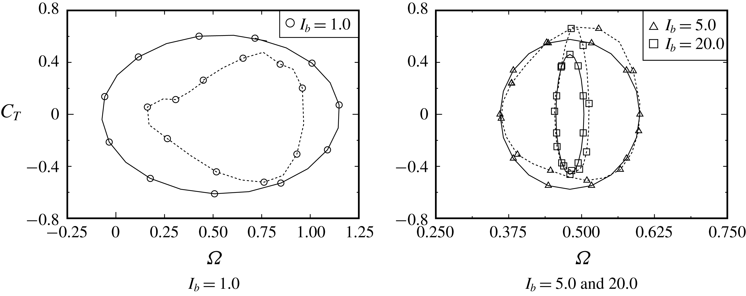
Start-up trajectories of
 $(C_{T},\unicode[STIX]{x1D6FA})$
until limit-cycle entry for
 $I_{b}=1.0$
,
 $5.0$
and
 $20.0$
. The limit cycles of figure 22 are depicted as dashed curves. Several typical stages, where the values of
 $\unicode[STIX]{x2202}_{\unicode[STIX]{x1D703}}C_{T}$
become zero, are depicted as
 $s_{0},s_{1},\ldots ,s_{9}$
. The trajectories start from the positions described as
 $t=0$
(i.e.
 $\unicode[STIX]{x1D703}(0)=90^{\circ }$
).

Start-up behaviours of
 $\exp (C_{T})$
(solid curve) and
 $\exp (\unicode[STIX]{x1D6FA})$
(dotted curve) in the polar coordinate system for
 $I_{b}=1.0$
,
 $5.0$
and
 $20.0$
. See figure 7 for
 $s_{0},s_{1},\ldots ,s_{9}$
. The rotor starts to rotate from the position of the solid symbol (i.e.
 $\unicode[STIX]{x1D703}(0)=90^{\circ }$
). The stable results of
 $\exp (C_{T})$
given in figure 18 are also drawn as thick dashed curves.


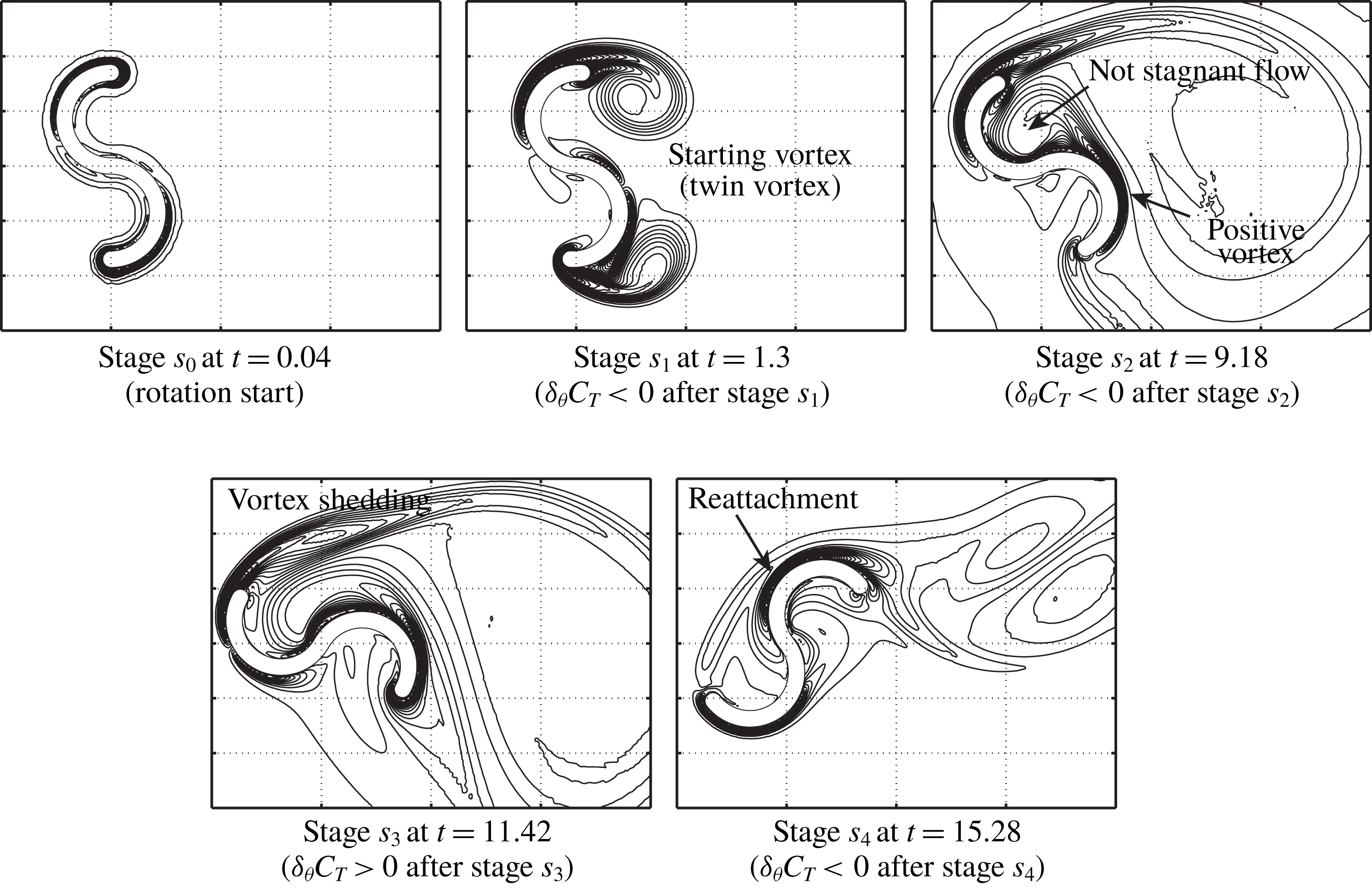


As seen on the left-hand side of figure 16, the stationary rotor starts to rotate at
 $t=0$
and ends up reaching the stable rotation successfully within a few cycles of the rotation for all values of
 $I_{b}$
. In figure 6, we can see the temporal start-up behaviours of
 $\unicode[STIX]{x1D6FA}(t)$
and
 $C_{T}(t)$
from the initial rotor angle of
 $\unicode[STIX]{x1D703}(0)=90^{\circ }$
.
3.2.1 Influence of MOI
Figure 7 shows the start-up trajectories of
 $C_{T}(t)$
with respect to
 $\unicode[STIX]{x1D6FA}(t)$
for
 $I_{b}=1.0$
,
 $5.0$
and
 $20.0$
until entering the limit cycle, which will be shown in figure 22. The initial rotor angle is set as
 $\unicode[STIX]{x1D703}(0)=90^{\circ }$
. The values of
 $\exp (C_{T})$
and
 $\exp (\unicode[STIX]{x1D6FA})$
shown in figure 7 are also plotted in figure 8 in the polar coordinate system. The positions of the stages
 $s_{1},s_{2},\ldots ,s_{9}$
, where
 $\unicode[STIX]{x2202}_{\unicode[STIX]{x1D6FA}}C_{T}=0$
is satisfied, are plotted in both figures 7 and 8 (for reference, these stages are also plotted in figure 6 for
 $I_{b}=5.0$
). Precisely, each stage is respectively defined as follows: (i) at stage
 $s_{0}$
, there is no vortex shedding from the rotor; (ii) at stages
 $s_{1}$
,
 $s_{2}$
,
 $s_{4}$
,
 $s_{6}$
and
 $s_{8}$
,
 $C_{T}$
exhibits the local maximum values after stage
 $s_{0}$
; and (iii) at stages
 $s_{3}$
,
 $s_{5}$
,
 $s_{7}$
and
 $s_{9}$
,
 $C_{T}$
exhibits the local minimum values after stage
 $s_{0}$
. As observed in figures 7 and 8, the value of
 $|C_{T}|$
rapidly increases in the clockwise direction from
 $t=0$
up to stage
 $s_{0}$
(i.e. the rotor rotates in the clockwise direction with
 $\unicode[STIX]{x1D6FA}<0$
at the extremely early stage of rotation) and then this value begins to decrease from stage
 $s_{0}$
. At the extremely early stage of rotation, vorticity forms near the rotor surface and, therefore, the inviscid and pseudo-steady discussion can account for the behaviours of
 $\unicode[STIX]{x1D6FA}$
and
 $C_{T}$
within the first few iterative steps. As will be seen at stage
 $s_{0}$
in figures 9–11, the vorticity is formed symmetrically between the tips of the upper and lower blades. Due to this vorticity, the negative pressure exerted on the inside surfaces of the rotor creates negative torque on the rotor so that it can rotate in the clockwise direction at the early stage. The extremely early stage of the rotation is discussed in detail in § 3.4. After stage
 $s_{1}$
, the trajectories approach each limit cycle, repeating between
 $C_{T}>0$
and
 $C_{T}<0$
(see figure 8). As observed in figures 7 and 8, the trajectories can be found to enter the limit cycle (i.e. stable rotation) within, at most, the first (for
 $I_{b}=1.0$
and
 $5.0$
) or second (for
 $I_{b}=20.0$
) cycles of the rotation.
Here, we set the start-up time as
 $t_{s}$
when the rotation reaches a limit cycle. Then, from the definitions of
 $\bar{\unicode[STIX]{x1D6FA}}$
and
 $\bar{C}_{T}$
(see (3.9)), we have, during one cycle of rotation,
 $$\begin{eqnarray}\displaystyle & \displaystyle \bar{\unicode[STIX]{x1D6FA}}=(1/T)\int _{t_{s}}^{t_{s}+T}\unicode[STIX]{x1D6FA}\,\text{d}t=(1/T)[\unicode[STIX]{x1D703}(t_{s}+T)-\unicode[STIX]{x1D703}(t_{s})], & \displaystyle\end{eqnarray}$$
 $$\begin{eqnarray}\displaystyle & \displaystyle \bar{C}_{T}=(1/T)\int _{t_{s}}^{t_{s}+T}C_{T}\,\text{d}t=(I_{b}/T)[\unicode[STIX]{x1D6FA}(t_{s}+T)-\unicode[STIX]{x1D6FA}(t_{s})]. & \displaystyle\end{eqnarray}$$
Differentiating equations (3.4) and (3.5) with respect to
 $t_{s}$
, we have the equation of motion based on the time-averaged variables:
 $$\begin{eqnarray}\text{d}\bar{\unicode[STIX]{x1D6FA}}/\text{d}t_{s}=\bar{C}_{T}(t_{s})/I_{b}.\end{eqnarray}$$
After the rotation reaches the limit cycle, the rotor rotates with a constant angular velocity as
 $\text{d}\bar{\unicode[STIX]{x1D6FA}}/\text{d}t_{s}=0$
, and then we have
 $\text{d}\bar{C}_{T}/\text{d}t_{s}=0$
from (3.5). Therefore, equation (3.6) gives the start-up time as
 $$\begin{eqnarray}t_{s}=I_{b}\int _{\bar{\unicode[STIX]{x1D6FA}}(0)}^{\bar{\unicode[STIX]{x1D6FA}}_{limit\text{-}cycle}}(1/\bar{C}_{T})\,\text{d}\bar{\unicode[STIX]{x1D6FA}},\end{eqnarray}$$
where
 $\bar{\unicode[STIX]{x1D6FA}}_{limit\text{-}cycle}$
indicates the average value after entering the limit cycle, and this value is estimated as approximately
 $0.5$
from table 1 and figure 16 for all values of
 $I_{b}$
. If the behaviour of
 $\bar{C}_{T}$
were independent of
 $I_{b}$
during start-up, the start-up time
 $t_{s}$
would increase with increasing
 $I_{b}$
, i.e. the rotor having a large value of
 $I_{b}$
is found to take a long time to reach stable rotation.
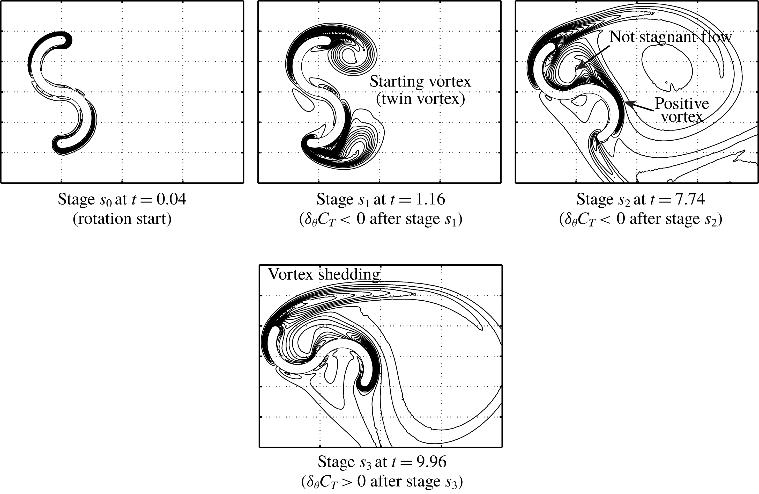
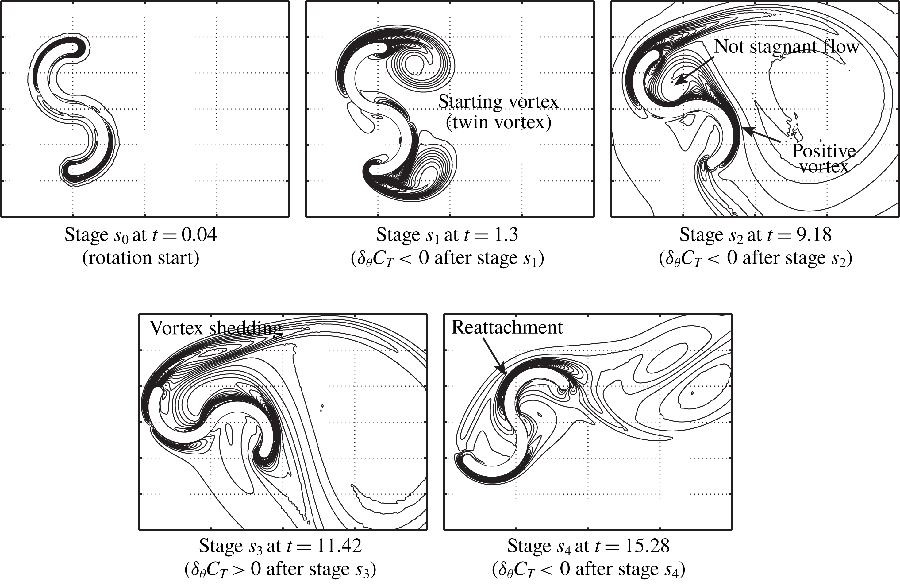
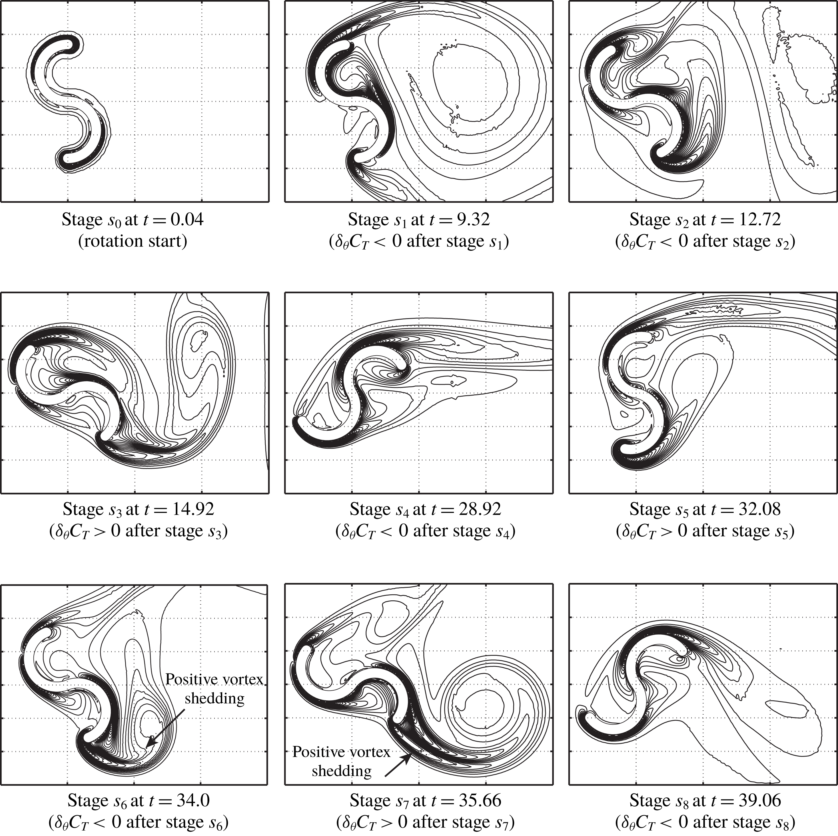
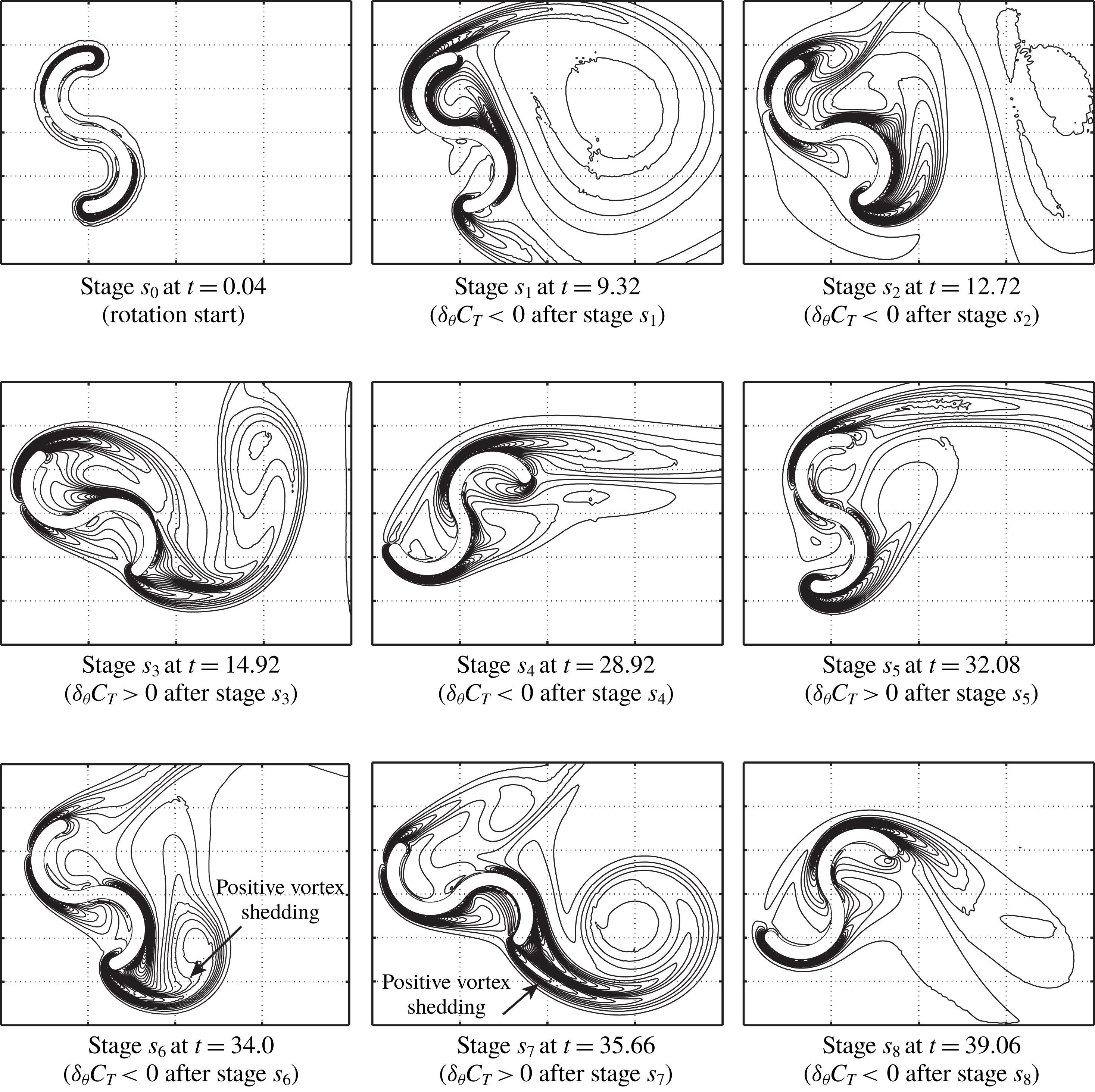
At stages
 $s_{0},s_{1},\ldots ,s_{8}$
, shown in figures 7 and 8, the iso-vorticity lines are presented for
 $I_{b}=1.0$
,
 $5.0$
and
 $20.0$
in figures 9, 10 and 11, respectively. At the beginning of rotation, the rotor marginally rotates in the clockwise direction from
 $\unicode[STIX]{x1D703}(0)=90^{\circ }$
(see figure 8) due to negative torque, which is caused by the initial vortices formed around the tips of the rotor (see stage
 $s_{0}$
in figures 9–11 and the above discussion).
With the growth of the vortex shedding from both tips of the two buckets (between stages
 $s_{0}$
and
 $s_{1}$
), the torque on the rotor rapidly decreases although the rotor continues to rotate in the clockwise direction. At around stage
 $s_{1}$
, the rotor turns in the counterclockwise direction. Between stages
 $s_{1}$
and
 $s_{2}$
, the twin vortex (i.e. starting vortex) behind the rotor grows. During these stages, the torque on the rotor is still not very large because
 $\exp (C_{T})\approx 1.0$
, as shown in figure 8. At stage
 $s_{2}$
, the positive vorticity generated from the surface of the returning bucket is observed, and it flows inside the advancing bucket because the rotor is almost stationary, although the vortex shedding from the tip of the advancing bucket begins to form (but its strength is weak). Therefore, the flow inside the advancing bucket is not stagnant, and the resultant negative pressure on the concave surface of this bucket can decrease the torque of the rotor, unlike the result of figure 20(i) during stable rotation. Then, the rotors having
 $I_{b}=1.0$
and
 $5.0$
repeatedly experience
 $\unicode[STIX]{x2202}_{\unicode[STIX]{x1D703}}C_{T}>0$
and
 $\unicode[STIX]{x2202}_{\unicode[STIX]{x1D703}}C_{T}<0$
and enter each limit cycle after stage
 $s_{3}$
for
 $I_{b}=1.0$
or stage
 $s_{4}$
for
 $I_{b}=5.0$
. In particular, the first vortex shedding from the advancing bucket, which is seen at stage
 $s_{3}$
, is found to play an important role in increasing the torque on the rotor. After stage
 $s_{4}$
(
 $I_{b}=5.0$
), the iso-vorticity line of figure 10 seems to be similar to that for the stable rotation shown in figure 20, although the trajectory has not completely entered the limit cycle yet at stage
 $s_{4}$
(see figure 7). In contrast, the rotor having
 $I_{b}=20.0$
starts to rotate slowly at the beginning and arrives at the limit cycle after stage
 $s_{9}$
(see figures 7 and 8). Because of the very slow rotation, the strong positive vortex shedding from the tip of the returning bucket can be observed at stages
 $s_{6}$
and
 $s_{7}$
, and this vortex shedding is found to delay limit-cycle entry (see figure 8).
Comparison of temporal growth of
 $\unicode[STIX]{x1D6FA}(t)$
from rotor start-up with various initial rotor angles
 $\unicode[STIX]{x1D703}(0)$
.

Start-up trajectories of
 $(C_{T},\unicode[STIX]{x1D6FA})$
until limit-cycle entry for the rotor with
 $I_{b}=5.0$
starting from
 $\unicode[STIX]{x1D703}(0)=\unicode[STIX]{x1D703}_{\unicode[STIX]{x1D6FA}_{min}}$
,
 $\unicode[STIX]{x1D703}_{C_{T}^{+}}$
and
 $\unicode[STIX]{x1D703}_{C_{T}^{-}}$
. The limit cycle of figure 22 is depicted as a dashed curve. Several typical stages where the values of
 $\unicode[STIX]{x2202}_{\unicode[STIX]{x1D703}}C_{T}$
become zero are depicted as
 $s_{0},s_{1},\ldots ,s_{6}$
. The rotor starts to rotate from the position described as
 $t=0$
.

Start-up behaviours of
 $\exp (C_{T})$
(solid curve) and
 $\exp (\unicode[STIX]{x1D6FA})$
(dotted curve) in the polar coordinate system for the rotor with
 $I_{b}=5.0$
starting from
 $\unicode[STIX]{x1D703}(0)=\unicode[STIX]{x1D703}_{\unicode[STIX]{x1D6FA}_{min}}$
,
 $\unicode[STIX]{x1D703}_{C_{T}^{+}}$
and
 $\unicode[STIX]{x1D703}_{C_{T}^{-}}$
. The rotor starts to rotate from the position of the solid symbol. The starting positions of
 $\exp (C_{T})$
for
 $\unicode[STIX]{x1D703}(0)=\unicode[STIX]{x1D703}_{C_{T}^{+}}$
and
 $\unicode[STIX]{x1D703}_{\unicode[STIX]{x1D6FA}_{min}}$
are omitted due to overlarge scales. See figure 13 for
 $s_{1},s_{1}^{\prime },\ldots ,s_{6}$
. The stable results of
 $\exp (C_{T})$
given in figure 18 are also depicted as thick dashed curves.

Iso-vorticity lines around the rotor with
 $I_{b}=5.0$
starting from
 $\unicode[STIX]{x1D703}(0)=\unicode[STIX]{x1D703}_{C_{T}^{+}}$
(left) and
 $\unicode[STIX]{x1D703}(0)=\unicode[STIX]{x1D703}_{C_{T}^{-}}$
(centre and right) at stages
 $s_{0}^{\prime }$
and
 $s_{1}^{\prime }$
(see figures 13 and 14).

3.2.2 Influence of initial rotor angle
To investigate the influence of the initial rotor angle
 $\unicode[STIX]{x1D703}(0)$
on the start-up, we selected three typical values of
 $\unicode[STIX]{x1D703}(0)=\unicode[STIX]{x1D703}_{\unicode[STIX]{x1D6FA}_{min}}$
,
 $\unicode[STIX]{x1D703}_{C_{T}^{+}}$
and
 $\unicode[STIX]{x1D703}_{C_{T}^{-}}$
, shown in table 1 and figure 20, together with
 $\unicode[STIX]{x1D703}(0)=90^{\circ }$
for which results are obtained in § 3.2.1. In this computation, the MOI is fixed at
 $I_{b}=5.0$
.
Figure 12 shows the temporal development of the angular velocity
 $\unicode[STIX]{x1D6FA}(t)$
from start-up at
 $t=0$
. Also, figure 13 shows the start-up trajectories into the limit cycle (see also figure 7 for
 $\unicode[STIX]{x1D703}(0)=90^{\circ }$
). As observed on the left-hand side of figure 18, the rotor experiences negative torque at both
 $\unicode[STIX]{x1D703}=\unicode[STIX]{x1D703}_{C_{T}^{-}}$
and
 $\unicode[STIX]{x1D703}=90^{\circ }$
, so that the rotor can rotate in the clockwise direction at the beginning of the start-up from
 $\unicode[STIX]{x1D703}(0)=\unicode[STIX]{x1D703}_{C_{T}^{-}}$
and
 $90^{\circ }$
. As seen in figure 13 together with figure 7, it is intriguing that the start-up trajectories for four values of
 $I_{p}$
arrive at the same limit cycle regardless of the different trajectories at start-up. Of course, the start-up time until entering the limit cycle from
 $t=0$
depends on the value of
 $\unicode[STIX]{x1D703}(0)$
(see table 2 and figure 13).
Figure 14 shows the start-up behaviours of
 $\exp (C_{T})$
and
 $\exp (\unicode[STIX]{x1D6FA})$
in the polar coordinate system for three values of
 $\unicode[STIX]{x1D703}(0)=\unicode[STIX]{x1D703}_{\unicode[STIX]{x1D6FA}_{min}}$
,
 $\unicode[STIX]{x1D703}_{C_{T}^{+}}$
and
 $\unicode[STIX]{x1D703}_{C_{T}^{-}}$
(see figure 8 for
 $\unicode[STIX]{x1D703}(0)=90^{\circ }$
). Several typical stages where the values of
 $\unicode[STIX]{x2202}_{\unicode[STIX]{x1D6FA}}C_{T}$
become zero are depicted in both figures 13 and 14 as
 $s_{0},s_{1},\ldots ,s_{6}$
. The times at which these stages are observed are listed in table 2. The flow patterns observed at these stages,
 $s_{0},s_{1},\ldots ,s_{6}$
, are confirmed to be similar to those of figures 9–11 for
 $\unicode[STIX]{x1D703}(0)=90^{\circ }$
. In figure 14, the additional stages
 $s_{0}^{\prime }$
and
 $s_{1}^{\prime }$
are observed at around
 $\unicode[STIX]{x1D703}=75^{\circ }$
and
 $90^{\circ }$
for
 $\unicode[STIX]{x1D703}(0)=\unicode[STIX]{x1D703}_{C_{T}^{+}}$
and
 $\unicode[STIX]{x1D703}_{C_{T}^{-}}$
. After stage
 $s_{2}$
, the previously mentioned start-up scenario for
 $\unicode[STIX]{x1D703}(0)=90^{\circ }$
(see e.g. figure 10 for
 $I_{b}=5.0$
) can essentially account for the start-up from
 $\unicode[STIX]{x1D703}(0)=\unicode[STIX]{x1D703}_{\unicode[STIX]{x1D6FA}_{min}}$
,
 $\unicode[STIX]{x1D703}_{C_{T}^{+}}$
and
 $\unicode[STIX]{x1D703}_{C_{T}^{-}}$
, as well. Therefore, the iso-vorticity lines appearing only at stages
 $s_{0}^{\prime }$
and
 $s_{1}^{\prime }$
, which cannot be observed in the result of
 $\unicode[STIX]{x1D703}(0)=90^{\circ }$
, are selected in figure 15 for
 $\unicode[STIX]{x1D703}(0)=\unicode[STIX]{x1D703}_{C_{T}^{+}}$
and
 $\unicode[STIX]{x1D703}_{C_{T}^{-}}$
. As described in table 1, the values of
 $\unicode[STIX]{x1D703}_{C_{T}^{+}}$
and
 $\unicode[STIX]{x1D703}_{C_{T}^{-}}$
are
 $30^{\circ }$
and
 $105^{\circ }$
, respectively.


On the rotor starting from
 $\unicode[STIX]{x1D703}(0)=\unicode[STIX]{x1D703}_{C_{T}^{+}}=30^{\circ }$
, the negative starting vortex shedding from the tip of the advancing bucket is sufficiently separated from the rotor at stage
 $s_{1}^{\prime }$
(where
 $\unicode[STIX]{x1D703}\approx 90^{\circ }$
) (see the left-hand side of figure 15) so that the flow inside the advancing bucket can be stagnant (it results in
 $\unicode[STIX]{x2202}_{\unicode[STIX]{x1D703}}C_{T}>0$
). Indeed, the initial iso-vorticity line at stage
 $s_{1}^{\prime }$
, shown on the left-hand side of figure 15, seems to be already similar to that for the stable regime at
 $\unicode[STIX]{x1D703}=\unicode[STIX]{x1D703}_{C_{T}^{-}}$
shown in figure 20(i). Therefore, the angular velocity
 $\unicode[STIX]{x1D6FA}$
, starting from
 $\unicode[STIX]{x1D703}(0)=\unicode[STIX]{x1D703}_{C_{T}^{+}}$
, monotonically increases at the beginning of start-up (see figure 12).
As for the rotor starting from
 $\unicode[STIX]{x1D703}(0)=\unicode[STIX]{x1D703}_{C_{T}^{-}}=105^{\circ }$
, at the beginning, the rotor rotates in the clockwise direction until
 $\unicode[STIX]{x1D703}\approx 75^{\circ }$
due to the initial negative torque, which is caused by the positive vorticity inside the advancing bucket (see figure 14 and the centre of figure 15). The rotor stops its rotation at
 $\unicode[STIX]{x1D703}=75^{\circ }$
, and immediately the angular velocity begins to increase in the counterclockwise direction, due to the stagnant flow inside the advancing bucket, from
 $\unicode[STIX]{x1D703}=75^{\circ }$
via stage
 $s_{1}^{\prime }$
(see the right-hand side of figure 15). In these additional two stages, the initial positive vorticity inside the advancing bucket is found to affect the sign of
 $\unicode[STIX]{x2202}_{\unicode[STIX]{x1D703}}C_{T}$
.
3.3 Flow-induced rotation of an S-shaped rotor after reaching stable rotation
In § 3.2, we considered the start-up mechanism where a stationary S-shaped rotor starts to rotate automatically due to a uniform flow. This subsection discusses the situation after the rotor has reached a stable rotation (i.e. entered a limit cycle, which will be mentioned in § 3.3.2), and investigates the torque supply mechanism for the rotor to sustain a stable rotation. In this subsection, the initial rotor angle
 $\unicode[STIX]{x1D703}(0)$
is fixed at
 $90^{\circ }$
.
3.3.1 Hydrodynamic characteristics
Figure 16 shows the temporal angular velocity of the rotor
 $\unicode[STIX]{x1D6FA}(t)$
and the torque coefficient
 $C_{T}(t)$
, together with the rotor angle
 $\unicode[STIX]{x1D703}(t)$
between
 $0^{\circ }$
and
 $360^{\circ }$
. The values of the MOI are selected as
 $I_{b}=1.0$
,
 $5.0$
and
 $20.0$
(numerical data are listed in table 1 for all MOI values). In figure 16, the temporal
 $\unicode[STIX]{x1D6FA}(t)$
and
 $C_{T}(t)$
are found to vary with two periods during one cycle of rotation because the rotor consists of two buckets. The rotor is supplied with torque from the fluid when
 $C_{T}>0$
(i.e. the rotor acts a turbine), whereas the rotor supplies torque to the fluid when
 $C_{T}<0$
(i.e. the rotor acts a pump). In particular, the behaviour of
 $C_{T}(t)$
after reaching stable rotation seems to be similar to the results of the predetermined constant rotation at
 $\unicode[STIX]{x1D706}=0.5$
(see figure 26 in appendix A). Besides, the angular velocity
 $\unicode[STIX]{x1D6FA}(t)$
varies temporally as well in the case of autorotation. As observed on the left-hand side of figure 16, the temporal
 $\unicode[STIX]{x1D6FA}(t)$
oscillates during one cycle of rotation, and the rotor with
 $I_{b}=1.0$
experiences a rapid acceleration and deceleration (i.e. sensitive response). As the value of
 $I_{b}$
increases, the oscillation amplitude of
 $\unicode[STIX]{x1D6FA}(t)$
decreases and the rotor achieves very smooth rotation at
 $I_{b}=20.0$
(see the value of
 $A_{\unicode[STIX]{x1D6FA}}$
, that is the amplitude of
 $\unicode[STIX]{x1D6FA}(t)$
, in table 1), whereas it takes a long time to reach stable rotation (this start-up has been already discussed in § 3.2).
Time variations of
 $\unicode[STIX]{x1D734}(t)$
(a,c,e) and
 $C_{T}(t)$
(b,d,f) together with the rotor angle
 $\unicode[STIX]{x1D703}(t)$
for three values of
 $I_{b}$
: (a,b)
 $I_{b}=1.0$
, (c,d)
 $I_{b}=5.0$
, (e,f)
 $I_{b}=20.0$
. Solid curve:
 $\unicode[STIX]{x1D734}(t)$
and
 $C_{T}(t)$
. Dotted curve:
 $\unicode[STIX]{x1D703}(t)$
.

Fast Fourier transform of
 $\unicode[STIX]{x1D734}(t)$
and
 $C_{T}(t)$
for three values of
 $I_{b}$
.

Equation (3.2) determines the angular velocity of the rotor and it can be rewritten in a dimensionless form, i.e.
 $$\begin{eqnarray}I_{b}\dot{\unicode[STIX]{x1D6FA}}=C_{T},\quad \dot{\unicode[STIX]{x1D703}}=\unicode[STIX]{x1D6FA}.\end{eqnarray}$$
Here, we define
 $\unicode[STIX]{x1D6FA}$
and
 $C_{T}$
averaged in time, during one cycle of rotation after reaching a stable state (i.e. limit cycle) at
 $t=t_{s}$
, as
 $$\begin{eqnarray}\bar{\unicode[STIX]{x1D6FA}}=\frac{1}{T}\int _{t_{s}}^{t_{s}+T}\unicode[STIX]{x1D6FA}\,\text{d}t,\quad \bar{C}_{T}=\frac{1}{T}\int _{t_{s}}^{t_{s}+T}C_{T}\,\text{d}t,\end{eqnarray}$$
where
 $T$
is the period of rotation. Then, after reaching a stable rotation, taking into account
 $$\begin{eqnarray}T\bar{\unicode[STIX]{x1D6FA}}=\int _{t_{s}}^{t_{s}+T}\unicode[STIX]{x1D6FA}\,\text{d}t=\int _{t_{s}}^{t_{s}+T}\dot{\unicode[STIX]{x1D703}}\,\text{d}t=\unicode[STIX]{x1D703}(t_{s}+T)-\unicode[STIX]{x1D703}(t_{s})=2\unicode[STIX]{x03C0},\end{eqnarray}$$
we readily have
 $T=2\unicode[STIX]{x03C0}/\bar{\unicode[STIX]{x1D6FA}}$
, i.e. the period of rotation
 $T$
can be found to be independent of
 $I_{b}$
if
 $\bar{\unicode[STIX]{x1D6FA}}$
is independent of
 $I_{b}$
. Furthermore, the value of
 $\bar{\unicode[STIX]{x1D6FA}}$
is approximately
 $0.5$
on the left-hand side of figure 16 and therefore we have
 $T=4\unicode[STIX]{x03C0}$
, whose value is found to be in agreement with the computed value of
 $T$
on the left-hand side of figure 16. This can be confirmed in the computed results plotted by the dashed curve in figure 16, which shows the temporal rotor angle. Also, the definition of
 $\bar{C}_{T}$
gives
 $$\begin{eqnarray}T\bar{C}_{T}=\int _{t_{s}}^{t_{s}+T}C_{T}\,\text{d}t=I_{b}\int _{t_{s}}^{t_{s}+T}\dot{\unicode[STIX]{x1D6FA}}\,\text{d}t=I_{b}[\unicode[STIX]{x1D6FA}(t_{s}+T)-\unicode[STIX]{x1D6FA}(t_{s})].\end{eqnarray}$$
We can therefore find
 $\bar{C}_{T}=0$
if the value of
 $\unicode[STIX]{x1D6FA}$
becomes the same in every period of rotation, i.e.
 $\unicode[STIX]{x1D6FA}(t_{s})=\unicode[STIX]{x1D6FA}(t_{s}+T)$
. Also, using (3.11) with
 $T=2\unicode[STIX]{x03C0}/\bar{\unicode[STIX]{x1D6FA}}$
and
 $\unicode[STIX]{x1D6FA}(t_{s}+T)+\unicode[STIX]{x1D6FA}(t_{s})\approx 2\bar{\unicode[STIX]{x1D6FA}}$
(see the left-hand side of figure 16), we have
 $$\begin{eqnarray}\unicode[STIX]{x1D6FA}(t_{s})=\bar{\unicode[STIX]{x1D6FA}}-\frac{\bar{C}_{T}}{I_{b}}\frac{T}{2},\quad \unicode[STIX]{x1D6FA}(t_{s}+T)=\bar{\unicode[STIX]{x1D6FA}}+\frac{\bar{C}_{T}}{I_{b}}\frac{T}{2}.\end{eqnarray}$$
Therefore, the angular velocity
 $\unicode[STIX]{x1D6FA}$
is found to vary in two periods during one cycle of rotation, i.e.
 $1/f_{\unicode[STIX]{x1D6FA}}=T/2$
(see the computed results of
 $f_{\unicode[STIX]{x1D6FA}}^{\ast }$
in table 1 and the right-hand side of figure 17). Furthermore, the value of
 $A_{\unicode[STIX]{x1D6FA}}$
, that is the amplitude of
 $\unicode[STIX]{x1D6FA}$
, can be found to decrease with an increase of
 $I_{b}$
if
 $\bar{C}_{T}$
is independent of
 $I_{b}$
(see the computed results of
 $A_{\unicode[STIX]{x1D6FA}}$
in table 1 and the left-hand side of figure 16).
The results of the fast Fourier transform spectrum of
 $\unicode[STIX]{x1D6FA}(t)$
and
 $C_{T}(t)$
, which is shown in figure 16 after stable rotation is reached, are shown in figure 17 for three values of
 $I_{b}=1.0$
,
 $5.0$
and
 $20.0$
(see table 1 for others). After reaching stable rotation, the rotor is found to sustain its own rotation mainly at the lowest frequency of
 $C_{T}(t)$
so that it can smoothly rotate with the lowest
 $\unicode[STIX]{x1D6FA}(t)$
. Solely at
 $I_{b}=1.0$
, two distinct frequencies in
 $\unicode[STIX]{x1D6FA}(t)$
can be observed in addition to the lowest one, although other strengths are relatively small compared with the lowest frequency. These high frequencies in
 $\unicode[STIX]{x1D6FA}(t)$
are caused by abrupt acceleration and deceleration of the rotor rotation. The values of the tip-speed ratio,
 $\unicode[STIX]{x1D706}=(2a_{1}-a_{3})\bar{\unicode[STIX]{x1D6FA}}(t)/V$
, are calculated as approximately
 $0.46$
for all values of
 $I_{b}$
using the values of the lowest frequency
 $f_{\unicode[STIX]{x1D6FA}}^{\ast }$
(see the values of
 $f_{\unicode[STIX]{x1D6FA}}^{\ast }$
in table 1). This value of
 $\unicode[STIX]{x1D706}\approx 0.46$
is also found to be in good agreement with the value of
 $\unicode[STIX]{x1D706}\approx 0.5$
shown in figure 25 for the computational results of the predetermined constant
 $\unicode[STIX]{x1D6FA}$
in appendix A. Integrating (3.8) from time
 $t_{1}$
to
 $t_{1}+T$
, we have
 $I_{b}\int _{t_{1}}^{t_{1}+T}\dot{\unicode[STIX]{x1D6FA}}\text{d}t=\int _{t_{1}}^{t_{1}+T}C_{T}\text{d}t=T\bar{C}_{T}$
, i.e.
 $I_{b}[\unicode[STIX]{x1D6FA}(t_{1}+T)-\unicode[STIX]{x1D6FA}(t_{1})]=T\bar{C}_{T}$
. Therefore, we can find
 $\bar{C}_{T}\approx 0$
in the limit cycle, which is confirmed in figures 16 and 18.
Comparison of the angle-averaged torque,
 $\exp (C_{T})$
, and the angular velocity,
 $\unicode[STIX]{x1D6FA}$
, in the polar coordinate system. Circles:
 $I_{b}=1.0$
. Triangles:
 $I_{b}=5.0$
. Squares:
 $I_{b}=20.0$
.

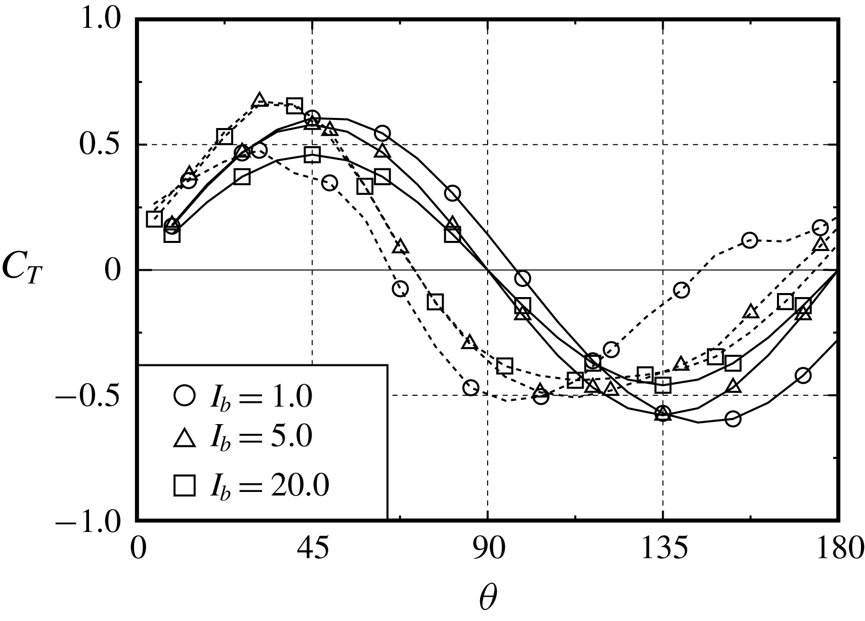
In figure 18, the values of
 $\exp (C_{T})$
and
 $\unicode[STIX]{x1D6FA}$
, which are averaged with respect to the rotor angle
 $\unicode[STIX]{x1D703}$
over more than
 $10$
cycles of rotation after reaching stable rotation, are plotted in the polar coordinate system for three values of
 $I_{b}=1.0$
,
 $5.0$
and
 $20.0$
. Here,
 $\exp (C_{T})\geqslant 1$
means
 $C_{T}\geqslant 0$
, and
 $\exp (C_{T})<1$
means
 $C_{T}<0$
. As observed, the rotor is supplied with the maximum torque from the fluid at around
 $\unicode[STIX]{x1D703}:=\unicode[STIX]{x1D703}_{C_{T}^{+}}=30^{\circ }$
(and
 $210^{\circ }$
), which then accelerates the rotation. The rotor rotates with the maximum
 $\unicode[STIX]{x1D6FA}$
at around
 $\unicode[STIX]{x1D703}:=\unicode[STIX]{x1D703}_{\unicode[STIX]{x1D6FA}_{max}}=70^{\circ }$
(and
 $250^{\circ }$
), and then decelerates in
 $\unicode[STIX]{x1D6FA}$
. The two buckets of the rotor yield two peaks in
 $C_{T}$
and
 $\unicode[STIX]{x1D6FA}$
. In contrast, at around
 $\unicode[STIX]{x1D703}:=\unicode[STIX]{x1D703}_{C_{T}^{-}}=105^{\circ }$
(and
 $285^{\circ }$
), the rotor is observed to supply the maximum torque to the fluid because the values of
 $\exp (C_{T})$
are less than unity. Due to the negative
 $C_{T}$
at
 $\unicode[STIX]{x1D703}:=\unicode[STIX]{x1D703}_{C_{T}^{-}}$
, the angular velocity
 $\unicode[STIX]{x1D6FA}$
exhibits the minimum value at around
 $\unicode[STIX]{x1D703}:=\unicode[STIX]{x1D703}_{\unicode[STIX]{x1D6FA}_{min}}=170^{\circ }$
(and
 $350^{\circ }$
). During stable rotation in the range between
 $\unicode[STIX]{x1D703}=0$
and
 $\unicode[STIX]{x1D703}=2\unicode[STIX]{x03C0}$
, because
 $I_{b}\unicode[STIX]{x1D6FA}(\text{d}\unicode[STIX]{x1D6FA}/\text{d}\unicode[STIX]{x1D703})=C_{T}$
, equation (3.8) can be written as
 $$\begin{eqnarray}\int _{0}^{2\unicode[STIX]{x03C0}}C_{T}\,\text{d}\unicode[STIX]{x1D703}=\frac{I_{b}}{2}[\unicode[STIX]{x1D6FA}^{2}(2\unicode[STIX]{x03C0})-\unicode[STIX]{x1D6FA}^{2}(0)]=0.\end{eqnarray}$$
The rotor is therefore found to rotate load-free in stable rotation (also see the left-hand side of figure 18). Indeed, the characteristics of
 $\exp (C_{T})$
for
 $I_{b}=5.0$
and
 $20.0$
seem to be similar to the result of
 $\unicode[STIX]{x1D706}=0.5$
, which exhibits
 $\bar{C}_{T}\approx 0$
, as shown in figure 27 (see appendix A).
Figure 19 shows the angle-averaged
 $\exp (C_{X})$
and
 $\exp (C_{Y})$
for
 $I_{b}=5.0$
in the polar coordinate system, together with
 $\exp (C_{T})$
from figure 18. Note that the small appropriate coefficients are multiplied to the values of
 $\exp (C_{X})$
and
 $\exp (C_{Y})$
to adjust their scale to match this figure (see the caption of figure 19). As observed, the strong
 $C_{Y}$
at
 $\unicode[STIX]{x1D703}:=\unicode[STIX]{x1D703}_{C_{Y}}\approx 165^{\circ }$
(and
 $345^{\circ }$
), instead of
 $C_{X}$
exhibiting the maximum value at
 $\unicode[STIX]{x1D703}:=\unicode[STIX]{x1D703}_{C_{X}}\approx 105^{\circ }$
(and
 $285^{\circ }$
), affects the subsequent positive torque at
 $\unicode[STIX]{x1D703}=\unicode[STIX]{x1D703}_{C_{T}^{+}}\approx 210^{\circ }$
(and
 $30^{\circ }$
). We here describe the components of the resultant force on the rotor in the
 $x$
- and
 $y$
-directions as
 $X$
and
 $Y$
and the point of application of the force as
 $(x_{f},y_{f})$
. The torque on the rotor, which is described as
 $T=x_{f}Y-y_{f}X$
, decreases to
 $T\approx x_{f}Y$
because of
 $Y\gg X$
. Taking into account the sign of
 $C_{Y}$
and
 $C_{T}$
with respect to
 $\unicode[STIX]{x1D703}$
in figure 19, we have
 $x_{f}<0$
, and therefore the point of application of force is found to locate on the downside of the rotor constantly, although
 $x_{f}\approx 0$
needs to be satisfied at
 $\unicode[STIX]{x1D703}\approx \unicode[STIX]{x1D703}_{C_{Y}}\approx 165^{\circ }$
.
Angle-averaged values of
 $0.015\exp (C_{X})$
(circles),
 $6.0\times 10^{-5}\exp (C_{Y})$
(triangles) and
 $\exp (C_{T})$
(squares) in the polar coordinate system for
 $I_{b}=5.0$
.

Pressure distributions
 $C_{p}$
on the rotor surface, iso-vorticity lines and streamlines at four selected stages for
 $I_{b}=5.0$
.

Figure 20 shows the computed pressure distributions
 $C_{p}$
on the rotor surface, the iso-vorticity lines and the streamlines at four selected values of rotor angle
 $\unicode[STIX]{x1D703}$
such that (i)
 $\unicode[STIX]{x1D703}=\unicode[STIX]{x1D703}_{C_{T}^{-}}\approx \unicode[STIX]{x1D703}_{C_{X}}$
, (ii)
 $\unicode[STIX]{x1D703}=\unicode[STIX]{x1D703}_{\unicode[STIX]{x1D6FA}_{min}}\approx \unicode[STIX]{x1D703}_{C_{Y}}$
, (iii)
 $\unicode[STIX]{x1D703}=\unicode[STIX]{x1D703}_{C_{T}^{+}}$
and (iv)
 $\unicode[STIX]{x1D703}=\unicode[STIX]{x1D703}_{\unicode[STIX]{x1D6FA}_{max}}$
. In figure 20, the value of
 $I_{b}$
is selected solely at
 $5.0$
and the flow patterns are of course confirmed to be similar to those of this figure among all values of computed
 $I_{b}$
(see table 1). The magnitude of the pressure,
 $C_{p}$
, is appropriately adjusted for legibility, although the definition of
 $C_{p}$
is given in (2.15). The patterns of the computed pressure distributions at
 $\unicode[STIX]{x1D703}=\unicode[STIX]{x1D703}_{\unicode[STIX]{x1D6FA}_{min}}$
and
 $\unicode[STIX]{x1D703}=\unicode[STIX]{x1D703}_{\unicode[STIX]{x1D6FA}_{max}}$
seem to be in good agreement with the experimental results of Fujisawa (Reference Fujisawa1992). Previous experimental studies of a Savonius rotor with a predetermined constant rotational velocity were carried out by Nakajima et al. (Reference Nakajima, Iio and Ikeda2008) and Fujisawa (Reference Fujisawa1992), and they partly observed the flow pattern shown in the present streamline.
According to Saffman (Reference Saffman1992), torque on a fluid domain
 ${\mathcal{D}}$
due to external force
 $\boldsymbol{F}$
(which is caused by rotor rotation in the present study) is given, in a two-dimensional absolute coordinate system, as
 $$\begin{eqnarray}\int _{{\mathcal{D}}}\boldsymbol{x}\wedge \boldsymbol{F}\text{d}S=-\frac{1}{2}\,\frac{\text{d}}{\text{d}t}\int _{{\mathcal{D}}}|\boldsymbol{x}|^{2}\unicode[STIX]{x1D714}\,\text{d}S.\end{eqnarray}$$
Therefore, the time variation of the vortex shedding from the rotor surface can be found to play a key role in torque generation on the rotor. At
 $\unicode[STIX]{x1D703}=\unicode[STIX]{x1D703}_{C_{T}^{-}}$
the approaching stream
 $V\boldsymbol{e}_{x}$
attaches to the convex surface of the advancing bucket and separates from the tip (see figure 20(i)). This vortex shedding from the tip of the advancing bucket affects the negative pressure distribution on the convex surface of the returning bucket as well as the concave surface of the advancing bucket (note that
 $\unicode[STIX]{x2202}_{\unicode[STIX]{x1D703}}C_{T}>0$
from
 $\unicode[STIX]{x1D703}=\unicode[STIX]{x1D703}_{C_{T}^{-}}$
). As the rotor rotates from
 $\unicode[STIX]{x1D703}=\unicode[STIX]{x1D703}_{C_{T}^{-}}$
in the counterclockwise direction, this vortex shedding is observed to reattach to the convex surface of the subsequent advancing bucket at
 $\unicode[STIX]{x1D703}=\unicode[STIX]{x1D703}_{C_{T}^{+}}$
(see figure 20(iii); note that
 $\unicode[STIX]{x2202}_{\unicode[STIX]{x1D703}}C_{T}<0$
from
 $\unicode[STIX]{x1D703}=\unicode[STIX]{x1D703}_{C_{T}^{+}}$
). Between
 $\unicode[STIX]{x1D703}=\unicode[STIX]{x1D703}_{C_{T}^{-}}$
and
 $\unicode[STIX]{x1D703}_{C_{T}^{+}}$
, due to the vortex shedding, the rotor surface on the side of the vortex shedding experiences a negative pressure (see figure 20(i) to (iii)), and this negative pressure on the convex surface can generate a positive torque on the rotor. After
 $\unicode[STIX]{x1D703}=\unicode[STIX]{x1D703}_{C_{T}^{+}}$
, the vortex shedding vanishes due to its reattachment, and therefore the convex surface of the advancing bucket experiences partly (weakly) the positive pressure at
 $\unicode[STIX]{x1D703}=\unicode[STIX]{x1D703}_{\unicode[STIX]{x1D6FA}_{max}}$
(see figure 20(iv)). After
 $\unicode[STIX]{x1D703}=\unicode[STIX]{x1D703}_{\unicode[STIX]{x1D6FA}_{max}}$
, the vortex shedding is repeatedly produced from the tip of the advancing bucket, as seen in figure 20(iv) to (i). Accordingly, the scenario can be summarized as follows. The vortex shedding from the tip of the advancing bucket, which is generated from
 $\unicode[STIX]{x1D703}=\unicode[STIX]{x1D703}_{C_{T}^{-}}$
to
 $\unicode[STIX]{x1D703}_{C_{T}^{+}}$
(see figure 20(i) to (iii)), can affect the increase of the torque of the rotor. Due to the reattachment of this vortex shedding on the subsequent advancing bucket at
 $\unicode[STIX]{x1D703}=\unicode[STIX]{x1D703}_{C_{T}^{+}}$
, the torque can decrease until
 $\unicode[STIX]{x1D703}=\unicode[STIX]{x1D703}_{C_{T}^{-}}$
of the subsequent rotation (see figure 20(iii) and (iv)). Owing to the present unsteady computation, the vortex shedding from the tip of the advancing bucket and its reattachment to the subsequent bucket can be found to play a key role in the increase and decrease of the torque on the rotor.
3.3.2 Limit cycle of an autonomous ordinary differential equation
Let us recall the equation of motion (3.2) for the SDOF problem of a rotor rotating automatically. When the torque
 $T_{r}$
depends solely on the angular velocity
 $\unicode[STIX]{x1D6FA}$
and rotor angle
 $\unicode[STIX]{x1D703}$
, equation (3.2) constructs the so-called autonomous system in a dimensionless form of
 $$\begin{eqnarray}\displaystyle & \displaystyle \dot{\unicode[STIX]{x1D703}}=\unicode[STIX]{x1D6FA}, & \displaystyle\end{eqnarray}$$
 $$\begin{eqnarray}\displaystyle & \displaystyle \dot{\unicode[STIX]{x1D6FA}}=(1/I_{b})\,C_{T}(\unicode[STIX]{x1D703},\unicode[STIX]{x1D6FA}), & \displaystyle\end{eqnarray}$$
where the dimensionless quantity of the MOI,
 $I_{b}$
, is based on
 $(1/16)\unicode[STIX]{x1D70C}D^{4}$
. We then set the perturbations
 $\unicode[STIX]{x0394}\unicode[STIX]{x1D703}$
and
 $\unicode[STIX]{x0394}\unicode[STIX]{x1D6FA}$
, from an equilibrium solution
 $(\unicode[STIX]{x1D703},\unicode[STIX]{x1D6FA})=(\unicode[STIX]{x1D703}^{\ast },\unicode[STIX]{x1D6FA}^{\ast })$
at
 $t=t^{\ast }$
, as
 $\unicode[STIX]{x0394}\unicode[STIX]{x1D703}=\unicode[STIX]{x1D703}-\unicode[STIX]{x1D703}^{\ast }$
and
 $\unicode[STIX]{x0394}\unicode[STIX]{x1D6FA}=\unicode[STIX]{x1D6FA}-\unicode[STIX]{x1D6FA}^{\ast }$
. The function
 $C_{T}$
is assumed to be a differentiable function at
 $(\unicode[STIX]{x1D703},\unicode[STIX]{x1D6FA})=(\unicode[STIX]{x1D703}^{\ast },\unicode[STIX]{x1D6FA}^{\ast })$
. Expanding
 $C_{T}(\unicode[STIX]{x1D703},\unicode[STIX]{x1D6FA})$
at
 $(\unicode[STIX]{x1D703}^{\ast },\unicode[STIX]{x1D6FA}^{\ast })$
with the use of the Taylor series, we then arrive, for the perturbations
 $(\unicode[STIX]{x0394}\unicode[STIX]{x1D703},\unicode[STIX]{x0394}\unicode[STIX]{x1D6FA})$
, at the following initial value problem for the autonomous system:
 $$\begin{eqnarray}\displaystyle & \displaystyle \dot{\unicode[STIX]{x1D723}}={\mathcal{A}}\unicode[STIX]{x1D723}+\boldsymbol{C}_{0}\quad \text{for }t>0\text{ and }t\neq t^{\ast }; & \displaystyle\end{eqnarray}$$
 $$\begin{eqnarray}\displaystyle & \displaystyle \dot{\unicode[STIX]{x1D723}}=\mathbf{0}\quad \text{at }t=t^{\ast }, & \displaystyle\end{eqnarray}$$
where the matrix
 ${\mathcal{A}}$
and vectors
 $\unicode[STIX]{x1D723}$
and
 $\boldsymbol{C}_{0}$
respectively stand for
 $$\begin{eqnarray}{\mathcal{A}}=\left[\begin{array}{@{}cc@{}}0 & 1\\ (1/I_{b})\unicode[STIX]{x2202}_{\unicode[STIX]{x1D703}}C_{T}|_{\unicode[STIX]{x1D703}=\unicode[STIX]{x1D703}^{\ast },\unicode[STIX]{x1D6FA}=\unicode[STIX]{x1D6FA}^{\ast }} & (1/I_{b})\unicode[STIX]{x2202}_{\unicode[STIX]{x1D6FA}}C_{T}|_{\unicode[STIX]{x1D703}=\unicode[STIX]{x1D703}^{\ast },\unicode[STIX]{x1D6FA}=\unicode[STIX]{x1D6FA}^{\ast }}\end{array}\right],\end{eqnarray}$$
 $$\begin{eqnarray}\unicode[STIX]{x1D723}=\left[\begin{array}{@{}c@{}}\unicode[STIX]{x0394}\unicode[STIX]{x1D703}\\ \unicode[STIX]{x0394}\unicode[STIX]{x1D6FA}\end{array}\right],\quad \boldsymbol{C}_{0}=\left[\begin{array}{@{}c@{}}\unicode[STIX]{x1D6FA}^{\ast }\\ (1/I_{b})C_{T}(\unicode[STIX]{x1D703}^{\ast },\unicode[STIX]{x1D6FA}^{\ast })\end{array}\right].\end{eqnarray}$$
The solution to (3.17)–(3.20) is given in appendix B. The roots of the characteristic polynomial of
 ${\mathcal{A}}$
give the eigenvalues
 $\unicode[STIX]{x1D706}=\unicode[STIX]{x1D706}_{1}$
and
 $\unicode[STIX]{x1D706}_{2}$
with
 $\unicode[STIX]{x1D706}_{1}>\unicode[STIX]{x1D706}_{2}$
:
 $$\begin{eqnarray}\displaystyle & \displaystyle \text{det}({\mathcal{A}}-\unicode[STIX]{x1D706}{\mathcal{E}})=\unicode[STIX]{x1D706}^{2}-a\unicode[STIX]{x1D706}-b=0\quad \text{i.e. }\unicode[STIX]{x1D706}_{1},\unicode[STIX]{x1D706}_{2}=a/2\pm \sqrt{D}, & \displaystyle\end{eqnarray}$$
 $$\begin{eqnarray}\displaystyle & \displaystyle \text{where }a=(1/I_{b})\unicode[STIX]{x2202}_{\unicode[STIX]{x1D6FA}}C_{T}|_{\unicode[STIX]{x1D703}=\unicode[STIX]{x1D703}^{\ast },\unicode[STIX]{x1D6FA}=\unicode[STIX]{x1D6FA}^{\ast }},b=(1/I_{b})\unicode[STIX]{x2202}_{\unicode[STIX]{x1D703}}C_{T}|_{\unicode[STIX]{x1D703}=\unicode[STIX]{x1D703}^{\ast },\unicode[STIX]{x1D6FA}=\unicode[STIX]{x1D6FA}^{\ast }},D=b+a^{2}/4. & \displaystyle \nonumber\\ \displaystyle & & \displaystyle\end{eqnarray}$$
 $\unicode[STIX]{x1D706}_{1}$
and
 $\unicode[STIX]{x1D706}_{2}$
are negative. As can be seen in the results of figure 16, there is no equilibrium solution
 $(\unicode[STIX]{x1D703}^{\ast },\unicode[STIX]{x1D6FA}^{\ast })$
where the angular velocity of the rotor
 $\unicode[STIX]{x1D6FA}$
tends to zero as
 $t\rightarrow \infty$
. In the following discussion, we thus seek a stable limit cycle in the phase-space structure. Furthermore, in § 3.4, the conditions of the rotor automatically starting up from a quiescent state and stopping from a stable rotation will be discussed based on the general solution to (3.17)–(3.21b
).
The Poincaré–Bendixon theorem. The Poincaré–Bendixon theorem states the long-time behaviour of trajectories of continuous dynamical systems on a plane, i.e. if, in a single-valued domain
 ${\mathcal{D}}_{0}$
, two continuous functions
 $f(x,y)$
and
 $g(x,y)$
are satisfied with
 $$\begin{eqnarray}\unicode[STIX]{x2202}_{x}f(x,y)+\unicode[STIX]{x2202}_{y}g(x,y)\neq 0,\end{eqnarray}$$
then a set of ordinary differential equations
 $$\begin{eqnarray}{\dot{x}}=f(x,y),\quad {\dot{y}}=g(x,y)\end{eqnarray}$$
does not have a closed trajectory in the domain
 ${\mathcal{D}}_{0}$
(see appendix C).
Comparison of (3.23) with (3.15) and (3.16) shows that the functions
 $f(x,y)$
and
 $g(x,y)$
are found to be replaced by
 $\unicode[STIX]{x1D6FA}$
and
 $(1/I_{b})C_{T}(\unicode[STIX]{x1D703},\unicode[STIX]{x1D6FA})$
, respectively. In contrast, in the Poincaré–Bendixon theorem the variables
 $x$
and
 $y$
(which relate to
 $\unicode[STIX]{x1D703}$
and
 $r$
of (3.15)–(3.16)) are involved in the semi-infinite domain
 $[0,\infty )$
of
 ${\mathcal{D}}_{0}$
. To switch the range of
 $x$
(i.e.
 $\unicode[STIX]{x1D703}$
) from
 $[0,\infty )$
to
 $[0,2\unicode[STIX]{x03C0}]$
, we introduce the polar coordinates of
 $(x,y)=(r\cos \unicode[STIX]{x1D703},r\sin \unicode[STIX]{x1D703})$
with
 $r=\exp [\unicode[STIX]{x1D6FA}(t)]$
and
 $\unicode[STIX]{x1D703}=[0,2\unicode[STIX]{x03C0}]$
and, then,
 $$\begin{eqnarray}\displaystyle & \displaystyle {\dot{x}}(=f(x,y))={\dot{r}}\cos \unicode[STIX]{x1D703}-r\dot{\unicode[STIX]{x1D703}}\sin \unicode[STIX]{x1D703}=(C_{T}/I_{b})x-(y/2)\log (x^{2}+y^{2}), & \displaystyle\end{eqnarray}$$
 $$\begin{eqnarray}\displaystyle & \displaystyle {\dot{y}}(=g(x,y))={\dot{r}}\sin \unicode[STIX]{x1D703}+r\dot{\unicode[STIX]{x1D703}}\cos \unicode[STIX]{x1D703}=(C_{T}/I_{b})y+(x/2)\log (x^{2}+y^{2}), & \displaystyle\end{eqnarray}$$
where
 $$\begin{eqnarray}{\dot{r}}=\dot{\unicode[STIX]{x1D6FA}}(t)\exp [\unicode[STIX]{x1D6FA}(t)]=(1/I_{b})rC_{T}(\log r,\unicode[STIX]{x1D703}),\quad \dot{\unicode[STIX]{x1D703}}=\log r.\end{eqnarray}$$
As mentioned in appendix C,
 $\unicode[STIX]{x2202}_{x}f+\unicode[STIX]{x2202}_{y}g=0$
is, in general, the necessary condition for the existence of a limit cycle in a single-valued problem. If a trajectory were to intersect a plane (i.e. the trajectory consists of a multi-cycle path), the condition of
 ${\dot{x}}={\dot{y}}=0$
would be fulfilled at the point of intersection (see appendix C). In the present problem, the condition for the existence of the intersection is described as
 $\dot{\unicode[STIX]{x1D703}}=\dot{\unicode[STIX]{x1D6FA}}=0$
. Then, the sum of (3.24) multiplied by
 $x$
and (3.25) multiplied by
 $y$
gives
 $(C_{T}/I_{b})r^{2}=0$
. Therefore, when the trajectory consists of a multi-cycle path, the condition of either
 $r=0$
or
 $C_{T}=0$
needs to be satisfied. The first condition of
 $r=0$
gives
 $x=y=0$
and this case makes no sense in the present problem. The second one of
 $C_{T}=0$
also gives
 $r=1$
from (3.24) or (3.25) and we can obtain
 $\dot{\unicode[STIX]{x1D703}}=\unicode[STIX]{x1D6FA}=0$
from (3.26). Therefore, it can be concluded that a trajectory consists of a single-cycle path (i.e. there is no intersection) if a limit cycle exists.
Using (3.24)–(3.25), we can calculate the left-hand side of (3.22) as
 $$\begin{eqnarray}\unicode[STIX]{x2202}_{x}f+\unicode[STIX]{x2202}_{y}g=(1/I_{b})(2C_{T}+x\unicode[STIX]{x2202}_{x}C_{T}+y\unicode[STIX]{x2202}_{y}C_{T})=(1/I_{b})(2C_{T}+r\unicode[STIX]{x2202}_{r}C_{T}).\end{eqnarray}$$
According to the Poincaré–Bendixon theorem, there is no limit cycle in the domain
 ${\mathcal{D}}_{0}$
if the right-hand side of (3.27) has a non-zero value. In the following discussion, we attempt to seek a limit cycle from this necessary condition for the existence of the limit cycle (i.e.
 $\unicode[STIX]{x2202}_{x}f+\unicode[STIX]{x2202}_{y}g=0$
) in the present problem.
As explained in appendix C, equation (3.27) relates to the source
 $m(r,\unicode[STIX]{x1D703})=(1/I_{b})(2C_{T}+r\unicode[STIX]{x2202}_{r}C_{T})$
in the domain
 ${\mathcal{D}}_{0}$
. Furthermore, the Poincaré–Bendixon theorem can be explained as follows. There exists a trajectory of a limit cycle if there exists a closed streamline
 $\unicode[STIX]{x1D6E4}$
which fulfils, in a single-valued domain
 ${\mathcal{D}}_{0}\supset \unicode[STIX]{x1D6E4}$
,
 $Q:=\iint _{{\mathcal{D}}_{0}}m(x,y)\,\text{d}x\,\text{d}y=0$
, where a normal velocity becomes zero on the closed streamline
 $\unicode[STIX]{x1D6E4}$
. Then, the trajectory of a limit cycle is identical to that of the closed streamline
 $\unicode[STIX]{x1D6E4}$
.
A total amount of the flow volume
 $Q$
induced by the source
 $m(r,\unicode[STIX]{x1D703})$
of (3.27) inside the domain
 ${\mathcal{D}}_{0}=\{r=r_{0}(\unicode[STIX]{x1D703}),0\leqslant \unicode[STIX]{x1D703}\leqslant 2\unicode[STIX]{x03C0}\}$
is calculated as
 $$\begin{eqnarray}Q=\int _{0}^{2\unicode[STIX]{x03C0}}\int _{0}^{r_{0}}m(r,\unicode[STIX]{x1D703})r\,\text{d}r\text{d}\unicode[STIX]{x1D703}=(1/I_{b})\int _{0}^{2\unicode[STIX]{x03C0}}\,\text{d}\unicode[STIX]{x1D703}\int _{0}^{r_{0}}\unicode[STIX]{x2202}_{r}(r^{2}C_{T})\,\text{d}r=(1/I_{b})\int _{0}^{2\unicode[STIX]{x03C0}}r_{0}^{2}C_{T}(r_{0},\unicode[STIX]{x1D703})\,\text{d}\unicode[STIX]{x1D703}.\end{eqnarray}$$
As mentioned above, there exists the trajectory of a limit cycle such that, if
 $Q=0$
, then the trajectory would be identical to the closed streamline
 $r=r_{0}(\unicode[STIX]{x1D703})$
. Since the trajectory of a limit cycle
 $r=r_{0}(\unicode[STIX]{x1D703})$
can be described in the form
 $r_{0}(\unicode[STIX]{x1D703})=\exp [\unicode[STIX]{x1D6FA}(\unicode[STIX]{x1D703})]$
, equation (3.28) can be rewritten as, noting that
 $C_{T}=I_{b}(\text{d}\unicode[STIX]{x1D6FA}(t)/\text{d}t)=I_{b}\unicode[STIX]{x1D6FA}(\text{d}\unicode[STIX]{x1D6FA}(\unicode[STIX]{x1D703})/\text{d}\unicode[STIX]{x1D703})$
from (3.16),
 $$\begin{eqnarray}Q=(1/I_{b})\int _{\unicode[STIX]{x1D6FA}(0)}^{\unicode[STIX]{x1D6FA}(2\unicode[STIX]{x03C0})}\unicode[STIX]{x1D6FA}e^{2\unicode[STIX]{x1D6FA}}\,\text{d}\unicode[STIX]{x1D6FA}=[1/(2I_{b})][\{\unicode[STIX]{x1D6FA}(2\unicode[STIX]{x03C0})-1/2\}\text{e}^{2\unicode[STIX]{x1D6FA}(2\unicode[STIX]{x03C0})}-\{\unicode[STIX]{x1D6FA}(0)-1/2\}\text{e}^{2\unicode[STIX]{x1D6FA}(0)}].\end{eqnarray}$$
The necessary condition,
 $Q=0$
, for the existence of a limit cycle gives
 $\unicode[STIX]{x1D6FA}(0)=\unicode[STIX]{x1D6FA}(2\unicode[STIX]{x03C0})$
, and therefore the angular velocity
 $\unicode[STIX]{x1D6FA}$
is found to be a periodic function with a period of
 $2\unicode[STIX]{x03C0}$
. Then, we can set the angular velocity
 $\unicode[STIX]{x1D6FA}$
in the form of (see also figure 17)
 $$\begin{eqnarray}\unicode[STIX]{x1D6FA}=\bar{\unicode[STIX]{x1D6FA}}+\mathop{\sum }_{n=1}^{\infty }A_{\unicode[STIX]{x1D6FA}n}\sin (2\unicode[STIX]{x03C0}nf_{\unicode[STIX]{x1D6FA}}^{\ast }t+\unicode[STIX]{x1D6FC}_{n}),\end{eqnarray}$$
where
 $A_{\unicode[STIX]{x1D6FA}n}$
and
 $\unicode[STIX]{x1D6FC}_{n}$
are indeterminate coefficients which are independent of
 $t$
. When
 $|A_{\unicode[STIX]{x1D6FA}n-1}|\gg |A_{\unicode[STIX]{x1D6FA}n}|$
can be assumed (this assumption is confirmed to be satisfied in the computational results of figure 17 in § 3.3.1), we can find
 $\unicode[STIX]{x1D703}\sim \bar{\unicode[STIX]{x1D6FA}}t$
as
 $t\rightarrow \infty$
. Therefore, in a limit cycle, equation (3.30) can be rewritten as
 $$\begin{eqnarray}\unicode[STIX]{x1D6FA}\sim \bar{\unicode[STIX]{x1D6FA}}+\mathop{\sum }_{n=1}^{\infty }A_{\unicode[STIX]{x1D6FA}n}\sin (2\unicode[STIX]{x03C0}n(f_{\unicode[STIX]{x1D6FA}}^{\ast }/\bar{\unicode[STIX]{x1D6FA}})\unicode[STIX]{x1D703}+\unicode[STIX]{x1D6FC}_{n}).\end{eqnarray}$$
For instance, the term
 $(f_{\unicode[STIX]{x1D6FA}}^{\ast }/\bar{\unicode[STIX]{x1D6FA}})$
fulfils, when
 $\unicode[STIX]{x1D6FA}$
is a periodic function with period of
 $T_{l}$
with respect to
 $\unicode[STIX]{x1D703}$
,
 $$\begin{eqnarray}f_{\unicode[STIX]{x1D6FA}}^{\ast }/\bar{\unicode[STIX]{x1D6FA}}=1/(nT_{l}),\quad \text{where }n=1,2,3,\ldots\end{eqnarray}$$
In addition, by substituting (3.31) into
 $C_{T}=I_{b}(\text{d}\unicode[STIX]{x1D6FA}(t)/\text{d}t)=I_{b}\unicode[STIX]{x1D6FA}(\text{d}\unicode[STIX]{x1D6FA}(\unicode[STIX]{x1D703})/\text{d}\unicode[STIX]{x1D703})$
of (3.16), the torque coefficient
 $C_{T}$
can be also expressed as, in a limit cycle,
 $$\begin{eqnarray}C_{T}\sim 2\unicode[STIX]{x03C0}I_{b}(f_{\unicode[STIX]{x1D6FA}}^{\ast }/\bar{\unicode[STIX]{x1D6FA}})\unicode[STIX]{x1D6FA}\mathop{\sum }_{n=1}^{\infty }nA_{\unicode[STIX]{x1D6FA}n}\cos (2\unicode[STIX]{x03C0}n(f_{\unicode[STIX]{x1D6FA}}^{\ast }/\bar{\unicode[STIX]{x1D6FA}})\unicode[STIX]{x1D703}+\unicode[STIX]{x1D6FC}_{n}),\end{eqnarray}$$
in which
 $\unicode[STIX]{x1D6FA}$
is also given by (3.31). Noting that
 $|A_{\unicode[STIX]{x1D6FA}1}|\gg |A_{\unicode[STIX]{x1D6FA}2}|\gg \cdots \,$
, the leading terms of
 $\unicode[STIX]{x1D6FA}$
and
 $C_{T}$
in (3.31) and (3.33) respectively reduce to
 $$\begin{eqnarray}\displaystyle & \displaystyle \unicode[STIX]{x1D6FA}-\bar{\unicode[STIX]{x1D6FA}}\sim A_{\unicode[STIX]{x1D6FA}1}\sin (2\unicode[STIX]{x03C0}(f_{\unicode[STIX]{x1D6FA}}^{\ast }/\bar{\unicode[STIX]{x1D6FA}})\unicode[STIX]{x1D703}+\unicode[STIX]{x1D6FC}_{1}), & \displaystyle\end{eqnarray}$$
 $$\begin{eqnarray}\displaystyle & \displaystyle C_{T}\sim 2\unicode[STIX]{x03C0}I_{b}(f_{\unicode[STIX]{x1D6FA}}^{\ast }/\bar{\unicode[STIX]{x1D6FA}})\bar{\unicode[STIX]{x1D6FA}}A_{\unicode[STIX]{x1D6FA}1}\cos (2\unicode[STIX]{x03C0}(f_{\unicode[STIX]{x1D6FA}}^{\ast }/\bar{\unicode[STIX]{x1D6FA}})\unicode[STIX]{x1D703}+\unicode[STIX]{x1D6FC}_{1}). & \displaystyle\end{eqnarray}$$
Therefore, equations (3.34) and (3.35) asymptotically give the trajectory of the limit cycle as
 $$\begin{eqnarray}[(\unicode[STIX]{x1D6FA}-\bar{\unicode[STIX]{x1D6FA}})/A_{\unicode[STIX]{x1D6FA}1}]^{2}+\{C_{T}/[2\unicode[STIX]{x03C0}I_{b}(f_{\unicode[STIX]{x1D6FA}}^{\ast }/\bar{\unicode[STIX]{x1D6FA}})\bar{\unicode[STIX]{x1D6FA}}A_{\unicode[STIX]{x1D6FA}1}]\}^{2}=1.\end{eqnarray}$$


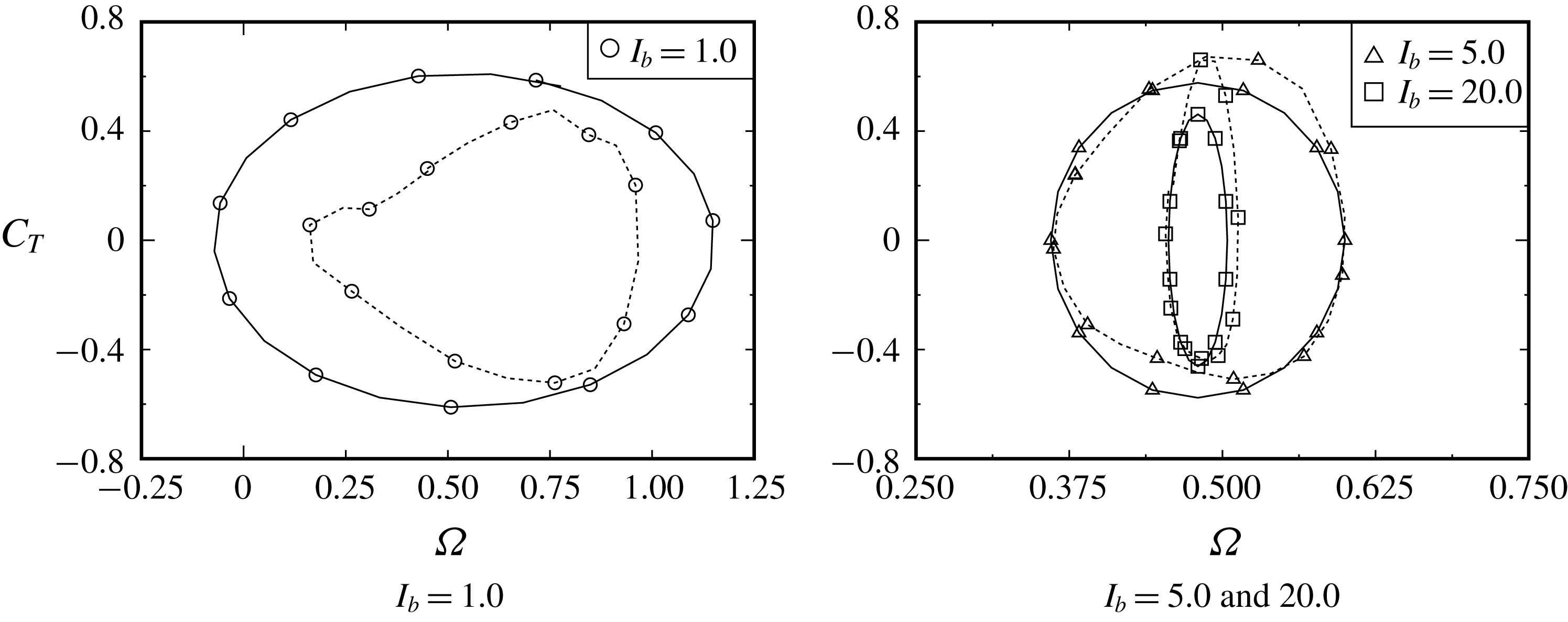
Let us verify the trajectory of (3.36) against the present computational results of § 3.3.1, where the rotation has reached a stable rotation. As mentioned above, the value of
 $A_{\unicode[STIX]{x1D6FA}1}$
can be approximately estimated by
 $A_{\unicode[STIX]{x1D6FA}}$
given in table 1, because of
 $|A_{\unicode[STIX]{x1D6FA}n-1}|\gg |A_{\unicode[STIX]{x1D6FA}n}|$
from figure 17. According to the values listed in table 1, the function
 $C_{T}$
of (3.35) is approximately written as
 $C_{T}\sim 0.61\cos (1.85\unicode[STIX]{x1D703}+\unicode[STIX]{x1D6FC}_{1})$
for
 $I_{b}=1.0$
,
 $C_{T}\sim 0.58\cos (2.00\unicode[STIX]{x1D703}+\unicode[STIX]{x1D6FC}_{1})$
for
 $I_{b}=5.0$
and
 $C_{T}\sim 0.46\cos (2.00\unicode[STIX]{x1D703}+\unicode[STIX]{x1D6FC}_{1})$
for
 $I_{b}=20.0$
. In figure 21, these functions of
 $C_{T}$
are compared with the computational results of § 3.3.1. The functions of
 $C_{T}$
are also observed to have a period
 $\unicode[STIX]{x03C0}$
with respect to
 $\unicode[STIX]{x1D703}$
because of the rotor consisting of two buckets. In figure 22, the trajectory of the limit cycle given by (3.36) is also compared with the computational results of § 3.3.1. For
 $I_{b}=5.0$
and
 $20.0$
, the computational results agree well with the trajectory of the limit cycle of (3.36). In contrast, for
 $I_{b}=1.0$
, the trajectory of (3.36) seems to be larger than that from the computational result. At
 $I_{b}=1.0$
, the angular velocity
 $\unicode[STIX]{x1D6FA}$
rapidly accelerates and decelerates during one cycle of the rotation (see figure 16(a,b)), so that the values of
 $A_{\unicode[STIX]{x1D6FA}2}$
and
 $A_{\unicode[STIX]{x1D6FA}3}$
cannot be assumed to be sufficiently smaller than the value of
 $A_{\unicode[STIX]{x1D6FA}1}$
(see figure 17). Therefore, the approximation of
 $|A_{\unicode[STIX]{x1D6FA}1}|\gg |A_{\unicode[STIX]{x1D6FA}2}|\gg \cdots \,$
adopted in (3.34) and (3.35) is invalid.
3.4 Investigation based on the general solution to the autonomous system
Let us investigate (i) the start-up behaviour of the S-shaped rotor from a quiescent state at
 $t=0$
and (ii) the condition of the rotor automatically stopping from a stable rotation, based on the general solution to the autonomous system in (3.17)–(3.20) and the eigenvalues of (3.21a
) and (3.21b
). The general solution to (3.17)–(3.20) is given in (B 4) with the coefficients of (B 5) and (B 6) in appendix B. In addition, we have supplementary relations of
 $\unicode[STIX]{x1D706}_{1}\unicode[STIX]{x1D706}_{2}=-b$
and
 $\unicode[STIX]{x1D706}_{1}-\unicode[STIX]{x1D706}_{2}=2\sqrt{D}$
from (3.21a
), together with
 $a=(1/I_{b})\unicode[STIX]{x2202}_{\unicode[STIX]{x1D6FA}}C_{T}|_{\unicode[STIX]{x1D703}=\unicode[STIX]{x1D703}^{\ast },\unicode[STIX]{x1D6FA}=\unicode[STIX]{x1D6FA}^{\ast }}$
,
 $b=(1/I_{b})\unicode[STIX]{x2202}_{\unicode[STIX]{x1D703}}C_{T}|_{\unicode[STIX]{x1D703}=\unicode[STIX]{x1D703}^{\ast },\unicode[STIX]{x1D6FA}=\unicode[STIX]{x1D6FA}^{\ast }}$
and
 $D=b+a^{2}/4$
of (3.21b
). Note here that the relations of (3.21a
) and (3.21b
) are invalid for the extremely early stage of the start-up because of the function
 $C_{T}$
not being smooth. The start-up at the extremely early stage will be discussed in (3.41)–(3.42).
(1) On start-up behaviour of
 $\unicode[STIX]{x0394}\unicode[STIX]{x1D6FA}$
. One sets
 $t^{\ast }=0$
and
 $\unicode[STIX]{x1D6FA}^{\ast }=0$
in (B 4), and then one gets
 $$\begin{eqnarray}\unicode[STIX]{x0394}\unicode[STIX]{x1D6FA}=[C_{T}/(I_{b}\sqrt{D})]\sinh (\sqrt{D}t)\exp [(a/2)t].\end{eqnarray}$$
For the start-up of the stationary rotor, the value of
 $\unicode[STIX]{x0394}\unicode[STIX]{x1D6FA}$
needs to be amplified over time. Then, one can classify (3.37) with respect to the sign of
 $D$
exhibiting either positive or negative value.
(i) For
 $D>0$
, equation (3.37) holds: (3.38)The angular velocity of the rotor is found to increase monotonically in the same direction as the torque.$$\begin{eqnarray}\unicode[STIX]{x0394}\unicode[STIX]{x1D6FA}=[C_{T}/(I_{b}\sqrt{D})]\sinh (\sqrt{D}t)\exp [(a/2)t].\end{eqnarray}$$
(ii) For
$D<0$
, equation (3.37) reduces to (3.39)The angular velocity of the rotor oscillates and its amplitude increases with time. According to the present computational results, the initial values of$$\begin{eqnarray}\unicode[STIX]{x0394}\unicode[STIX]{x1D6FA}=[C_{T}/(I_{b}\sqrt{-D})]\sin (\sqrt{-D}t)\exp [(a/2)t].\end{eqnarray}$$
$D$
are negative for all the selected values of
$\unicode[STIX]{x1D703}(0)$
. At the beginning of start-up,
$\unicode[STIX]{x0394}\unicode[STIX]{x1D6FA}$
is therefore found to increase in the same direction of
$C_{T}$
because of
$\sin (\sqrt{-D}t)\approx \sqrt{-D}t>0$
for
$t\ll 1$
.




In both conditions of (3.38) and (3.39),
 $\unicode[STIX]{x0394}\unicode[STIX]{x1D6FA}$
can be found to behave like, at the beginning of start-up, taking into account
 $\sinh (\sqrt{D}t)\approx \sqrt{D}t$
for
 $t\ll 1/\sqrt{D}$
and
 $\exp (at/2)\approx 1$
for
 $t\ll 2/a$
,
 $$\begin{eqnarray}\unicode[STIX]{x0394}\unicode[STIX]{x1D6FA}\approx (C_{T}/I_{b})t.\end{eqnarray}$$
Equation (3.40) can be valid immediately after the rotor starts to rotate in the counterclockwise direction, although the rotor starts to rotate in the clockwise direction at the extremely early stage of start-up. As observed in figures 8 and 16, the rotor starts to rotate in the clockwise direction at the extremely early stage. As discussed in (3.41), the function of
 $C_{L}$
is not continuous with respect to
 $\unicode[STIX]{x1D6FA}$
at this early stage of the start-up. We therefore remove this situation from the consideration of (3.40). During the early stage for
 $t\ll 1$
, as seen in figure 23, the torque coefficient
 $C_{T}$
decreases with time as
 $$\begin{eqnarray}C_{T}\approx c_{0}t^{-\unicode[STIX]{x1D6FC}},\end{eqnarray}$$
where the values of the coefficient
 $c_{0}$
and the exponent
 $-\unicode[STIX]{x1D6FC}$
can be determined by fitting with the computed results in figure 23. Note that the coefficient
 $c_{0}$
takes either positive values for
 $\unicode[STIX]{x1D703}(0)=\unicode[STIX]{x1D703}_{C_{T}^{+}}$
and
 $\unicode[STIX]{x1D703}_{\unicode[STIX]{x1D6FA}_{min}}$
or negative values for
 $\unicode[STIX]{x1D703}(0)=90^{\circ }$
and
 $\unicode[STIX]{x1D703}_{C_{T}^{-}}$
, i.e.
 $c_{0}\approx 1.5$
and
 $\unicode[STIX]{x1D6FC}\approx 0.15$
for
 $\unicode[STIX]{x1D703}(0)=\unicode[STIX]{x1D703}_{C_{T}^{+}}$
and
 $\unicode[STIX]{x1D703}_{\unicode[STIX]{x1D6FA}_{min}}$
;
 $c_{0}\approx -0.5$
and
 $\unicode[STIX]{x1D6FC}\approx 0.4$
for
 $\unicode[STIX]{x1D703}(0)=\unicode[STIX]{x1D703}_{C_{T}^{-}}$
; and
 $c_{0}\approx -0.3$
and
 $\unicode[STIX]{x1D6FC}\approx 0.4$
for
 $\unicode[STIX]{x1D703}(0)=90^{\circ }$
. At the beginning of start-up, the value of
 $\unicode[STIX]{x0394}\unicode[STIX]{x1D6FA}$
can be found to develop with time by substituting (3.41) into (3.40) as
 $$\begin{eqnarray}\unicode[STIX]{x0394}\unicode[STIX]{x1D6FA}\approx (c_{0}/I_{b})t^{1-\unicode[STIX]{x1D6FC}}.\end{eqnarray}$$
Comparison of initial behaviours of
 $|C_{T}(t)|$
for four values of the initial rotor angle
 $\unicode[STIX]{x1D703}(0)$
together with the fitting equations of (3.41).

(2) On the condition of automatically stopping. One sets
 $t=t^{\ast }$
and
 $\unicode[STIX]{x1D6FA}^{\ast }=0$
in (B 4), and then one replaces
 $t$
by
 $t-t^{\ast }$
in (3.37). For the automatic stopping of a stably rotating rotor at
 $t=t^{\ast }$
, the condition of
 $a<0$
and
 $b<0$
needs to be satisfied (i.e.
 $\text{Re}[\unicode[STIX]{x1D706}_{1}]<0$
and
 $\text{Re}[\unicode[STIX]{x1D706}_{2}]<0$
for a stable condition), and this leads to the following behaviours of
 $\unicode[STIX]{x0394}\unicode[STIX]{x1D6FA}$
at
 $t=t^{\ast }$
.
- (iii)
In the condition of
$a<0$
and
$b<0$
(with
$D>0$
), (3.37) holds: (3.43)$$\begin{eqnarray}\unicode[STIX]{x0394}\unicode[STIX]{x1D6FA}=[C_{T}/(I_{b}\sqrt{D})]\sinh (\sqrt{D}(t-t^{\ast }))\exp [(a/2)(t-t^{\ast })].\end{eqnarray}$$
The angular velocity monotonically decreases in the same direction as the torque from a stably rotating regime.
- (iv)
In the condition of
$a<0$
and
$b<0$
(with
$D<0$
), (3.37) reduces to (3.44)$$\begin{eqnarray}\unicode[STIX]{x0394}\unicode[STIX]{x1D6FA}=[C_{T}/(I_{b}\sqrt{-D})]\sin (\sqrt{-D}(t-t^{\ast }))\exp [(a/2)(t-t^{\ast })].\end{eqnarray}$$
The angular velocity decreases with time from a stably rotating regime with the oscillation.


Figure 24 plots the values of
 $\exp (a)$
and
 $\exp (b)$
in the polar coordinate system for stable rotation at
 $I_{b}=5.0$
. These values are calculated from the results of figure 18 in which the present autonomous system has entered the limit cycle of figure 22. Note that in this computation the value of
 $D=b+a^{2}/4$
is positive for all values of
 $\unicode[STIX]{x1D703}$
. As seen in figure 24, this system behaves stably when both of the coefficients
 $a$
and
 $b$
are negative (coloured in grey), whereas the non-shaded region does not fulfil the stable condition. Therefore, this autonomous system is found to maintain its limit cycle repeatedly between the stable and non-stable states during one cycle of rotation.
Values of
 $\exp (a)$
(circle) and
 $\exp (b)$
(triangle) in the polar coordinate system for the stably rotating rotor with
 $I_{b}=5.0$
, as calculated from the values of figure 18. The scales for
 $\exp (a)$
values are enlarged.

4 Conclusions
The present work has investigated an unsteady flow over an S-shaped rotor automatically rotating from a quiescent state using a remeshed vortex particle method. Such a flow-induced rotation of the rotor which is impulsively immersed in a constant flow is still an unclear phenomenon. This work has shed light on the limit cycle in the present autonomous system and successfully elucidated the mechanism of the autorotation of the rotor.
This work first verified the adopted vortex particle method. In particular, the computational procedure of the pressure on the surface of a body was successfully verified about an abruptly started circular cylinder with and without rotation against the previous analytical and numerical results.
Sections 3.2, 3.3 and 3.4 investigated the problem whereby the S-shaped rotor automatically starts to rotate from a quiescent state. The rotor is assumed to be a load-free rotor. Section 3.2 focused on the situation during start-up. During rotor start-up, which was discussed in § 3.2, the trajectories until entering the limit cycle were given for
 $I_{b}=1.0$
,
 $5.0$
and
 $20.0$
, starting from
 $\unicode[STIX]{x1D703}(0)=90^{\circ }$
. The initial rotor angle
 $\unicode[STIX]{x1D703}(0)$
was also varied using three values where
 $C_{T}$
exhibits the positive and negative maximum values and
 $\unicode[STIX]{x1D6FA}$
exhibits the minimum value. The S-shaped rotor was confirmed to approach the same limit cycle with increasing time for all selected values of
 $I_{b}$
and
 $\unicode[STIX]{x1D703}(0)$
, although the values of
 $I_{b}$
and
 $\unicode[STIX]{x1D703}(0)$
affect the distance of the trajectory to the limit cycle (i.e. the start-up time). Owing to the computed iso-vorticity line at the beginning of start-up, the first vortex shedding from the advancing bucket plays an important role in increasing the torque on the rotor, after which the trajectory enters the limit cycle.
Section 3.3 focused on the situation after the rotor reached stable rotation. As described in this subsection, rotors having various MOI
 $I_{b}$
were initially set at
 $\unicode[STIX]{x1D703}(0)=90^{\circ }$
. The torque coefficient
 $C_{T}$
and the angular velocity
 $\unicode[STIX]{x1D6FA}$
were plotted in the polar coordinate system during one cycle of the rotation, and then the pressure distributions on the rotor surface, the iso-vorticity lines and the streamlines were given at specific rotor angles. Owing to the present unsteady computation, the vortex shedding from the tip of the advancing bucket and its reattachment to the subsequent bucket were found to play a key role in increasing and decreasing the torque on the rotor.
In § 3.3.2, a remarkable finding is the fact that the autonomous system can account for the flow-induced rotation of the rotor. Indeed, the trajectory of a limit cycle based on the Poincaré–Bendixon theorem was derived theoretically and compared with the present computational results after the rotor reached stable rotation. Furthermore, at
 $I_{b}=1.0$
, the acceleration and deceleration of
 $\unicode[STIX]{x1D6FA}$
during one cycle of the rotation were found to affect the trajectory of the limit cycle.
According to § 3.4, to successfully start up and sustain the rotation of a rotor, the initial torque caused by the first vortex shedding from the advancing bucket was found to be important and it initially behaves like
 $C_{T}\sim -t^{-0.4}$
for
 $\unicode[STIX]{x1D703}(0)=90^{\circ }$
and
 $\unicode[STIX]{x1D703}_{C_{T}^{-}}$
and
 $C_{T}\sim t^{-0.15}$
for
 $\unicode[STIX]{x1D703}(0)=\unicode[STIX]{x1D703}_{C_{T}^{+}}$
and
 $\unicode[STIX]{x1D703}_{\unicode[STIX]{x1D6FA}_{min}}$
. After entering the limit cycle, the present autonomous system was found to maintain the rotation repeatedly between the stable and non-stable states during one rotation cycle.
In the present study, additional structures such as springs and dampers were not considered. For an actual VAWT, the influence of the damper, which relates to a dynamo-electric generator, has a key role in the performance. Therefore, it is intended to investigate the influence of damping in future work.
Appendix A. Impulsively started rotating S-shaped rotor with predetermined constant angular velocity
At
 $t\rightarrow +0$
, the rotor
 ${\mathcal{C}}_{b}$
is impulsively immersed in uniform velocity
 $V\boldsymbol{e}_{x}$
with
 $V>0$
and rotates with the predetermined constant angular velocity
 $\unicode[STIX]{x1D6FA}\boldsymbol{e}_{z}$
in the counterclockwise direction from the initial rotor angle of
 $\unicode[STIX]{x1D703}(0)=90^{\circ }$
(see figure 4). To simulate this problem, we select the same computational parameters as in § 3.3. The computation is carried out up to
 $t=2Vt_{0}/D=176$
when the stable oscillation of
 $C_{T}(t)$
exceeds
 $40$
periods.
This computation selects five kinds of tip-speed ratios:
 $\unicode[STIX]{x1D706}=2a_{1}\unicode[STIX]{x1D6FA}/V=0.0$
,
 $0.25$
,
 $0.5$
,
 $0.75$
and
 $1.0$
. Figure 25 shows the time-averaged torque characteristic of the rotor with constant angular velocities, that is calculated by
 $\bar{C}_{T}=[1/(t(N_{s}+N)-t(N_{s}))]\int _{t(N_{s})}^{t(N_{s}+N)}C_{T}(t)\,\text{d}t$
. Here,
 $N_{s}(=2)$
indicates the number of rotations when it saturates the transient flow caused by the impulsive rotation from
 $t=0$
, and the values of
 $C_{T}$
are averaged over
 $N(=5)$
rotations. The computation of
 $\unicode[STIX]{x1D706}=0.0$
is carried out for the stationary rotor with a rotor angle of
 $\unicode[STIX]{x1D703}=90^{\circ }$
. As observed in this figure, the torque varies from positive to negative at
 $\unicode[STIX]{x1D706}\approx 0.5$
; i.e. the rotor is supplied with torque from the fluid when
 $\unicode[STIX]{x1D706}\lessapprox 0.5$
.
Time-averaged torque coefficient
 $\bar{C}_{T}$
versus tip-speed ratio
 $\unicode[STIX]{x1D706}$
for predetermined constant angular velocities
 $\unicode[STIX]{x1D6FA}$
.

Comparison of temporal variations of the torque on the rotor among
 $\unicode[STIX]{x1D706}=0.25$
,
 $0.5$
and
 $0.75$
. Solid curve:
 $C_{T}(t)$
. Dotted curve: rotor angle
 $\unicode[STIX]{x1D703}(t)$
.

Figure 26 shows the temporal variations of the torque coefficient
 $C_{T}(t)$
and the rotor angle
 $\unicode[STIX]{x1D703}(t)$
for
 $\unicode[STIX]{x1D706}=0.25$
,
 $0.5$
and
 $0.75$
. In figure 26, the value of
 $C_{T}$
is observed to vary with two periods during one cycle of rotation because the rotor consists of two buckets (note that at
 $\unicode[STIX]{x1D706}=0.25$
another frequency appears in the value of
 $C_{T}$
; see also the right-hand side of figure 27). Furthermore, as observed in figure 26, the time-averaged torque
 $\bar{C}_{T}$
for
 $\unicode[STIX]{x1D706}=0.75$
exhibits negative values, and therefore this rotor supplies torque to the fluid (this rotor acts a pump). In contrast with
 $\unicode[STIX]{x1D706}=0.75$
, the rotor with
 $\unicode[STIX]{x1D706}=0.25$
experiences only positive torque and is found to act as a turbine. Figure 27 shows the values of
 $\exp (C_{T})$
in the polar coordinate system for
 $\unicode[STIX]{x1D706}=0.5$
,
 $0.75$
and
 $0.25$
. For
 $\unicode[STIX]{x1D706}=0.5$
, the rotor is supplied with torque from the fluid between
 $\unicode[STIX]{x1D703}\approx 0^{\circ }$
and
 $70^{\circ }$
, whereas the rotor supplies torque to the fluid between
 $\unicode[STIX]{x1D703}\approx 70^{\circ }$
and
 $180^{\circ }$
. In particular, the torque coefficient
 $C_{T}$
exhibits the maximum value at around
 $\unicode[STIX]{x1D703}=40^{\circ }$
and
 $220^{\circ }$
, which is in good agreement with the experimental results of Ushiyama et al. (Reference Ushiyama, Nagai and Shinoda1986) for the static torque coefficient measured with a wind tunnel. In contrast with
 $\unicode[STIX]{x1D706}=0.5$
, almost all values of
 $\unicode[STIX]{x1D706}=0.75$
seem to be plotted inside the unit circle because
 $C_{T}\lessapprox 0$
for all values of
 $\unicode[STIX]{x1D703}$
. Unlike
 $\unicode[STIX]{x1D706}=0.5$
and
 $0.75$
, the rotor with
 $\unicode[STIX]{x1D706}=0.25$
gives two peaks in the value of
 $C_{T}$
(see the right-hand side of figure 27 and also figure 26) and supplies no more torque to the fluid in all rotor angles (i.e.
 $\exp (C_{T})\gtrapprox 1$
for all values of
 $\unicode[STIX]{x1D703}$
). Figures 28 and 29 show the pressure distributions on the rotor
 $C_{p}$
, the iso-vorticity lines and the streamlines at two values of the rotor angle:
 $\unicode[STIX]{x1D703}=\unicode[STIX]{x1D703}_{C_{T}^{-}}$
and
 $\unicode[STIX]{x1D703}=\unicode[STIX]{x1D703}_{C_{T}^{+}}$
, where
 $C_{T}$
exhibits a maximum negative value at
 $\unicode[STIX]{x1D703}=\unicode[STIX]{x1D703}_{C_{T}^{-}}$
(
 $\unicode[STIX]{x2202}_{\unicode[STIX]{x1D703}}C_{T}>0$
for
 $\unicode[STIX]{x1D703}>\unicode[STIX]{x1D703}_{C_{T}^{-}}$
) and a maximum positive value at
 $\unicode[STIX]{x1D703}=\unicode[STIX]{x1D703}_{C_{T}^{+}}$
(
 $\unicode[STIX]{x2202}_{\unicode[STIX]{x1D703}}C_{T}<0$
for
 $\unicode[STIX]{x1D703}>\unicode[STIX]{x1D703}_{C_{T}^{+}}$
) (see also figure 27). As observed in the streamlines of figure 28, at
 $\unicode[STIX]{x1D703}=\unicode[STIX]{x1D703}_{C_{T}^{-}}$
, the approaching uniform stream
 $V\boldsymbol{e}_{x}$
attaches to the convex surface of the advancing bucket and separates from the tip. The value of
 $C_{T}$
seems to begin to increase (i.e.
 $\unicode[STIX]{x2202}_{\unicode[STIX]{x1D703}}C_{T}>0$
for
 $\unicode[STIX]{x1D703}>\unicode[STIX]{x1D703}_{C_{T}^{-}}$
) due to the negative pressure distribution on the convex surface of the returning bucket when the vortex shedding from the tip of the advancing bucket appears. In contrast, at
 $\unicode[STIX]{x1D703}=\unicode[STIX]{x1D703}_{C_{T}^{+}}$
(see figure 29), the vortex shedding seems to reattach to the convex surface of the subsequent advancing bucket (i.e. the flow inside the returning bucket might be stagnant), and therefore the rotor surface on the side of the vortex shedding experiences a negative pressure, which causes the positive torque of the rotor.
Comparison of angle-averaged torque,
 $\exp (C_{T})$
, on the rotor rotating with a constant
 $\unicode[STIX]{x1D6FA}$
in the polar coordinate system among
 $\unicode[STIX]{x1D706}=0.5$
(circles),
 $\unicode[STIX]{x1D706}=0.75$
(triangles) and
 $\unicode[STIX]{x1D706}=0.25$
(circles).

The detailed phenomenon related to figures 28 and 29 was also discussed in § 3.3.1.
(a–c) Pressure distributions
 $C_{p}$
on the rotor surface, (d–f) iso-vorticity lines and (g–i) streamlines at the rotor angle of
 $\unicode[STIX]{x1D703}=\unicode[STIX]{x1D703}_{C_{T}^{-}}$
(
 $\unicode[STIX]{x2202}_{\unicode[STIX]{x1D703}}C_{T}>0$
for
 $\unicode[STIX]{x1D703}>\unicode[STIX]{x1D703}_{C_{T}^{-}}$
).

(a–c) Pressure distributions
 $C_{p}$
on the rotor surface, (d–f) iso-vorticity lines and (g–i) streamlines at the rotor angle of
 $\unicode[STIX]{x1D703}=\unicode[STIX]{x1D703}_{C_{T}^{+}}$
(
 $\unicode[STIX]{x2202}_{\unicode[STIX]{x1D703}}C_{T}<0$
for
 $\unicode[STIX]{x1D703}>\unicode[STIX]{x1D703}_{C_{T}^{+}}$
).

Appendix B. Solution to autonomous system, equations (3.17)–(3.20)
Let us derive the general solution to (3.17)–(3.20). We rewrite (3.17) as the set of
 $$\begin{eqnarray}\displaystyle & \displaystyle \unicode[STIX]{x2202}_{t}(\unicode[STIX]{x0394}\unicode[STIX]{x1D703})=\unicode[STIX]{x1D6FA}^{\ast }+\unicode[STIX]{x0394}\unicode[STIX]{x1D6FA}, & \displaystyle\end{eqnarray}$$
 $$\begin{eqnarray}\displaystyle & \displaystyle \unicode[STIX]{x2202}_{t}(\unicode[STIX]{x0394}\unicode[STIX]{x1D6FA})=(1/I_{b})[\unicode[STIX]{x2202}_{\unicode[STIX]{x1D703}}C_{T}(\unicode[STIX]{x1D703}^{\ast },\unicode[STIX]{x1D6FA}^{\ast })\unicode[STIX]{x0394}\unicode[STIX]{x1D703}+\unicode[STIX]{x2202}_{\unicode[STIX]{x1D6FA}}C_{T}(\unicode[STIX]{x1D703}^{\ast },\unicode[STIX]{x1D6FA}^{\ast })\unicode[STIX]{x0394}\unicode[STIX]{x1D6FA}+C_{T}(\unicode[STIX]{x1D703}^{\ast },\unicode[STIX]{x1D6FA}^{\ast })]. & \displaystyle\end{eqnarray}$$
Differentiating (B 2) with respect to
 $t$
and substituting it into (B 1), we have
 $$\begin{eqnarray}I_{b}\unicode[STIX]{x2202}_{t}^{2}(\unicode[STIX]{x0394}\unicode[STIX]{x1D6FA})=\unicode[STIX]{x2202}_{\unicode[STIX]{x1D6FA}}C_{T}(\unicode[STIX]{x1D703}^{\ast },\unicode[STIX]{x1D6FA}^{\ast })\unicode[STIX]{x2202}_{t}(\unicode[STIX]{x0394}\unicode[STIX]{x1D6FA})+\unicode[STIX]{x2202}_{\unicode[STIX]{x1D703}}C_{T}(\unicode[STIX]{x1D703}^{\ast },\unicode[STIX]{x1D6FA}^{\ast })(\unicode[STIX]{x1D6FA}^{\ast }+\unicode[STIX]{x0394}\unicode[STIX]{x1D6FA}).\end{eqnarray}$$
The general solution to (B 3) reads, with indeterminate coefficients
 $A_{1}$
and
 $A_{2}$
,
 $$\begin{eqnarray}\unicode[STIX]{x0394}\unicode[STIX]{x1D6FA}=A_{1}\exp (\unicode[STIX]{x1D706}_{1}t)+A_{2}\exp (\unicode[STIX]{x1D706}_{2}t)-\unicode[STIX]{x1D6FA}^{\ast }.\end{eqnarray}$$
The indeterminate coefficients can be successfully determined, using the initial condition (3.18) and the characteristic polynomial (3.21a ), as
 $$\begin{eqnarray}\displaystyle & \displaystyle A_{1}=\left[\frac{\unicode[STIX]{x1D706}_{1}}{\unicode[STIX]{x1D706}_{1}-\unicode[STIX]{x1D706}_{2}}\unicode[STIX]{x1D6FA}^{\ast }+{\displaystyle \frac{\unicode[STIX]{x1D706}_{1}\unicode[STIX]{x1D706}_{2}}{\unicode[STIX]{x1D706}_{1}-\unicode[STIX]{x1D706}_{2}}}{\displaystyle \frac{(\unicode[STIX]{x2202}_{\unicode[STIX]{x1D6FA}}C_{T}/\unicode[STIX]{x2202}_{\unicode[STIX]{x1D703}}C_{T})\unicode[STIX]{x1D6FA}^{\ast }-C_{T}}{\unicode[STIX]{x2202}_{\unicode[STIX]{x1D703}}C_{T}}}\right]\exp (-\unicode[STIX]{x1D706}_{1}t^{\ast }), & \displaystyle\end{eqnarray}$$
 $$\begin{eqnarray}\displaystyle & \displaystyle A_{2}=-\left[\frac{\unicode[STIX]{x1D706}_{2}}{\unicode[STIX]{x1D706}_{1}-\unicode[STIX]{x1D706}_{2}}\unicode[STIX]{x1D6FA}^{\ast }+{\displaystyle \frac{\unicode[STIX]{x1D706}_{1}\unicode[STIX]{x1D706}_{2}}{\unicode[STIX]{x1D706}_{1}-\unicode[STIX]{x1D706}_{2}}}{\displaystyle \frac{(\unicode[STIX]{x2202}_{\unicode[STIX]{x1D6FA}}C_{T}/\unicode[STIX]{x2202}_{\unicode[STIX]{x1D703}}C_{T})\unicode[STIX]{x1D6FA}^{\ast }-C_{T}}{\unicode[STIX]{x2202}_{\unicode[STIX]{x1D703}}C_{T}}}\right]\exp (-\unicode[STIX]{x1D706}_{2}t^{\ast }). & \displaystyle\end{eqnarray}$$
Appendix C. Discussion of the Poincaré–Bendixon theorem
The Poincaré–Bendixon theorem is expressed in (3.22)–(3.23). Using Green’s theorem and Gauss’ divergence theorem in a single-valued domain
 ${\mathcal{D}}_{0}$
, one can write
 $$\begin{eqnarray}\iint _{{\mathcal{D}}_{0}}(\unicode[STIX]{x2202}_{x}f+\unicode[STIX]{x2202}_{y}g)\,\text{d}x\,\text{d}y=\int _{\unicode[STIX]{x2202}{\mathcal{D}}_{0}}(f\,\text{d}y-g\,\text{d}x).\end{eqnarray}$$
If there exists a limit cycle
 $\unicode[STIX]{x1D6E4}$
in domain
 ${\mathcal{D}}_{0}$
, one selects
 ${\mathcal{D}}_{0}$
which satisfies
 $\unicode[STIX]{x1D6E4}=\unicode[STIX]{x2202}{\mathcal{D}}_{0}$
, and then one can calculate the right-hand side of (C 1) as
 $$\begin{eqnarray}\int _{\unicode[STIX]{x2202}{\mathcal{D}}_{0}}(f\,\text{d}y-g\,\text{d}x)=\int _{\unicode[STIX]{x1D6E4}}(f{\dot{y}}-g{\dot{x}})\,\text{d}t=\int _{\unicode[STIX]{x1D6E4}}(fg-gf)\,\text{d}t=0.\end{eqnarray}$$
The assumption of (3.22) in the Poincaré–Bendixon theorem prohibits the left-hand side of (C 2) from being zero. Therefore, there exists no limit cycle if (3.22) were fulfilled. In other words, fulfilling
 $\unicode[STIX]{x2202}_{x}f+\unicode[STIX]{x2202}_{y}g=0$
is the necessary condition for the existence of a limit cycle.
If a limit cycle exists and its trajectory is written by
 $(x(s),y(s))$
with the position
 $s\in [s_{o},s_{e})$
, one can write
 $x(s_{o})=x(s_{e})$
,
 $y(s_{o})=y(s_{e})$
and, on the trajectory of the limit cycle,
 $$\begin{eqnarray}\displaystyle & \displaystyle \text{d}x/\text{d}t= & \displaystyle (\text{d}x/\text{d}s)(\text{d}s/\text{d}t)=f(x(s),y(s))=f(s),\end{eqnarray}$$
 $$\begin{eqnarray}\displaystyle & \displaystyle \text{d}y/\text{d}t= & \displaystyle (\text{d}y/\text{d}s)(\text{d}s/\text{d}t)=g(x(s),y(s))=g(s).\end{eqnarray}$$
By combining (C 3) and (C 4), one can obtain
 $$\begin{eqnarray}g\frac{\text{d}x}{\text{d}s}-f\frac{\text{d}y}{\text{d}s}=\left(\frac{\text{d}y}{\text{d}s}\frac{\text{d}x}{\text{d}s}-\frac{\text{d}x}{\text{d}s}\frac{\text{d}y}{\text{d}s}\right)\frac{\text{d}s}{\text{d}t}=0.\end{eqnarray}$$
Note that the Poincaré–Bendixon theorem is applicable to a single-valued problem. For a multi-valued problem that the trajectory intersects, one needs to cut the plane to separate it into single-valued planes. The multi-valued problem appears when
 $\text{d}s/\text{d}t=0$
is satisfied in (C 5) and, at the intersection, it fulfils
 ${\dot{x}}={\dot{y}}=0$
.
One can replace
 $f$
and
 $g$
by the velocities
 $u$
and
 $v$
in (3.23). Then, the left-hand side of (3.22) can be found to represent a pathline:
 $$\begin{eqnarray}\unicode[STIX]{x2202}_{x}u+\unicode[STIX]{x2202}_{y}v:=m(x,y),\end{eqnarray}$$
in which
 $m(x,y)$
is a source term in the domain
 ${\mathcal{D}}_{0}$
, as will be discussed below. Note that in an autonomous system, the velocities
 $(u,v)$
are time-invariant and the pathline is therefore identical to the streamline (i.e. the trajectory of (3.17)–(3.20) represents the streamline). Using (C 6), one can rewrite (3.22) and link it to the flow volume
 $Q$
inside the single-valued domain
 ${\mathcal{D}}_{0}$
:
 $$\begin{eqnarray}Q:=\iint _{{\mathcal{D}}_{0}}m(x,y)\,\text{d}x\,\text{d}y\neq 0.\end{eqnarray}$$
To satisfy (C 7), there exists no closed trajectory in domain
 ${\mathcal{D}}_{0}$
(see the Poincaré–Bendixon theorem), i.e. if the flow volume
 $Q$
were to have a non-zero value, a closed curve inside
 ${\mathcal{D}}_{0}$
would not be a streamline. Therefore, a closed streamline, which fulfils
 $Q=0$
, can account for the trajectory of a limit cycle as follows. There exists a trajectory of a limit cycle which is identical to a streamline if there exists a closed streamline
 $\unicode[STIX]{x1D6E4}$
which fulfils, in a single-valued domain
 ${\mathcal{D}}_{0}\supset \unicode[STIX]{x1D6E4}$
,
 $$\begin{eqnarray}Q=\iint _{{\mathcal{D}}_{0}}\left(\frac{\unicode[STIX]{x2202}f}{\unicode[STIX]{x2202}x}+\frac{\unicode[STIX]{x2202}g}{\unicode[STIX]{x2202}y}\right)\,\text{d}x\,\text{d}y=\int _{\unicode[STIX]{x2202}{\mathcal{D}}_{0}=\unicode[STIX]{x1D6E4}}\left(f\frac{\text{d}y}{\text{d}s}-g\frac{\text{d}x}{\text{d}s}\right)\,\text{d}s=0,\end{eqnarray}$$
where the normal velocity becomes zero on the closed streamline
 $\unicode[STIX]{x1D6E4}$
surrounding the source
 $m(x,y)=\unicode[STIX]{x2202}_{x}f+\unicode[STIX]{x2202}_{y}g$
.
In summary, one can find the following:
(i)
$\unicode[STIX]{x2202}_{x}f+\unicode[STIX]{x2202}_{y}g=0$
, i.e.
$Q=0$
is the necessary condition for the existence of a limit cycle.(ii) The trajectory having a multi-cycle path gives
$\text{d}s/\text{d}t=0$
, i.e.
${\dot{x}}={\dot{y}}=0$
at the intersection.


Here we consider a simple example for the limit cycle which is obtained from the following system (this example is cited from Takahashi Reference Takahashi1996):
 $$\begin{eqnarray}{\dot{x}}=u=y+x(1-x^{2}-y^{2}),\quad {\dot{y}}=v=-x+y(1-x^{2}-y^{2}).\end{eqnarray}$$
From (C 6), the strength of the source is calculated as
 $m=1-3(x^{2}+y^{2})=1-3r^{2}$
, and therefore one can consider a closed domain inside a circle having a radius of
 $r_{0}$
. Similar to (C 8), one calculates the total amount of the flow volume
 $Q$
inside the domain of
 $r=r_{0}$
, i.e.
 $$\begin{eqnarray}Q=\int _{0}^{2\unicode[STIX]{x03C0}}\text{d}\unicode[STIX]{x1D703}\int _{0}^{r_{0}}m(r)r\,\text{d}r=2\unicode[STIX]{x03C0}(r_{0}-r_{0}^{3})=0.\end{eqnarray}$$
Equation (C 10) gives the closed streamline of the unit circle (
 $r_{0}=1$
). This unit circle can be found to be the trajectory of the limit cycle of (C 9).