1 Introduction
Using Unmanned Aerial Vehicles (UAV) has become a major trend in first responder, security and defense areas. UAV navigation plans are generally defined during mission preparation. However, during mission preparation or execution, different users can request for additional observations to be performed by the UAV. It is then necessary to insert these actions in UAV navigation plans. The user must deal with constraints that will impact the overall plan feasibility, such as observation preconditions, duration of the UAV mission or resource consumption. For example, a rotorcraft can easily perform an observation using stationary flight, but has poor endurance. In turn, a fixed wing can perform longer missions but needs to orbit around a waypoint to acquire and observe a target. This paper addresses vehicle planning issues, managing constraints composed of mission objectives, execution time and resource requirements. In this problem, UAVs can communicate with the network to transmit remote videos to ground manned vehicles on ground.
The optimization problem consists in finding the path that maximizes the overall mission efficiency while ensuring mission duration and resource consumption. The structure of consumption and observation constraints make the problem difficult to model and hard to solve. Determining the shortest path may not lead to the most efficient one, since observation requests may occur for various different places. The paper proposes a constraint model for UAV activity optimization, before and during mission execution. It is formulated as a Constraint Satisfaction Problem (CSP), and implemented using the Constraint Logic Programming (CLP) framework over Finite Domains (FD). The constraint-based model combines flow constraints over {0,1} variables, with resource constraints and conditional task activation models. A solving method is also proposed, which tends to be a very generic approach for solving these complex problems. It is based on Branch and Bound (B&B), constraint propagation and a probing technique. Probing is a search strategy that manages the state space solver exploration using the solution of a low-computational relaxed problem evaluation. Results are reported using a SICStus Prolog CLP(FD) implementation, with performances that suit operational needs.
The first section introduces the problem and the second one describes our constraint-based approach, compared with the state of the art. Next section presents problem formulation as a CSP. Search algorithms are then described. We give a few results on realistic benchmarks and a general conclusion.
2 Unmanned Aerial Vehicles mission planning problem
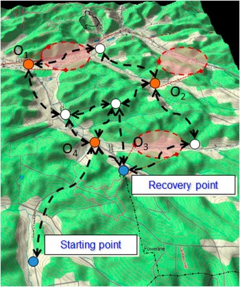
Intrinsic UAV characteristics (i.e. maximal speed, manoeuvrability, practical altitudes) have a direct impact on operation efficiency. Figure 1 presents the Patroller, a UAV that has large wingspan to allow medium altitude flight, which enables performing long-range missions by minimizing energy consumption. UAV operations are not only constrained by energetic resources, but also mission time and terrain structure. Figure 2 shows a set of potential waypoints to flyby. They are defined during mission preparation, by terrain analysis, mission objectives and situation assessment. Navigation constraints are also defined by available corridors, that are provided either by navigation authorities, in civilian space, or by the Air Command Order, in military context.
The patroller unmanned aerial vehicles (UAV) can detect targets at long range. With such UAV, the operator requests observation at preparation time or during mission execution

Navigation plan and observation requests from users. The unmanned aerial vehicles must maximize the number of requested observations (specified by field of views, represented in red), under time and energetic constraints

2.1 Informal description
A navigation plan consists in a subset of waypoints, totally ordered, estimated flyby dates and some observations to perform. Choosing the final mission plan depends on multiple criteria (duration, available energy, exposure, objectives, initial and recovery points). Maximizing mission objectives, for instance the number of observations performed during the mission, is the primary cost objective of planning automation. The overall mission duration, exposure and on-board energy may also be maintained as low as possible. To decide a mission plan, the user must deal with the following elements:
-
∙ Initial UAV conditions: initial positions and remaining energy.
-
∙ Terrain structure: defined as a set of navigation waypoints, connected by available paths. Each waypoint has a geographical reference, and a distance metric is defined to compute the value between any couple of waypoints.
-
∙ Mission objectives: the final recovery point, and any waypoint to which a sensing observation has been associated (requested by some user).
-
∙ On-board resource consumption: resources can be consumed due to UAV mobility (from a waypoint to another one) and/or observation action.
-
∙ Exposure: in some defense missions, the UAV exposure to threats shall be mastered.
In general, the plan is defined at mission preparation time, but it can be redefined online due to the situation evolution:
-
∙ Situation changes: new threats might appear.
-
∙ Mission objective: sensing and observations actions can be updated. The recovery points can be updated during mission execution.
-
∙ UAV state: energy consumption is not what was expected (for instance due to wind conditions).
The remote operator receives in real time all the critical data that may require a replanning event. To be able to keep operational efficiency, it is fundamental to have fast solving algorithms that can address realistic missions plans and be able to deal with all the mission constraints.
2.2 Example
In Figure 2, the UAV takes off from the initial position (blue circle) and must perform a maximal set of observations among {O 1, O 2, O 3, O 4}. Each observation consumes energy and time, as for navigation between two points. In case of a defense mission, it also exposes the UAV to opponent visibility. The UAV is recovered after a last potential observation in O 3 (blue circle). To satisfy energy and UAV exposure, the user decides to only plan for observation actions {O 1, O 2, O 3} and discards observation O 4. White circles are potential flyby navigation points.
2.3 Complexity
Some simplified versions of the problem are equivalent to known hard problems. If the set of observations is fixed, then the problem can be specialized as a Travelling Salesman Problem with multiple distance constraints. Maximizing the set of observation actions can also be relaxed as a knapsack problem by formulating a path weight for each action. In both cases, these problems are known to be non polynomial (NP)-hard, and solution verification can be performed in polynomial time. Solution can be evaluated by a simple check of the navigation plan, verifying that each action is correctly scheduled and metrics are correctly instantiated. Therefore some problem instances are NP-hard on worst cases, although polynomial families may certainly be exhibited.
3 A constraint programming approach
3.1 State of the art
Several approaches can deal with such problems, ranging from classical planning to very specific algorithms:
-
∙ Domain-independent planning (Fox & Long, Reference Fox and Long2000), using Planning Domain Description Language formalisms (Fox & Long, Reference Fox and Long2003). This language can model several complex actions.
-
∙ Dedicated planners have been developed for UAV, unmanned ground vehicle and vehicle planning: Ix-TeT (Laborie & Ghallab, Reference Laborie and Ghallab1995), Heuristic Scheduling Testbed System (Muscettola, Reference Muscettola1993), Reactive Model-based Programming Language (Abramson et al., Reference Abramson, Kim and Williams2001).
-
∙ Planning frameworks like Hierarchical Task Network (Goldman et al., Reference Goldman, Haigh, Musliner and Pelican2002; Meuleau et al., Reference Meuleau, Plaunt, Smith and Smith2009) have been developed to tackle specific operational domains.
All these framework need to be complemented with CSP formulation in order to tackle resource and temporal constraints. Linear Programming (LP) techniques can also be envisaged. However, if dealing with nonlinearity or discrete variables, constraints cannot be easily reformulated into linear ones without a massive increase of the variable set.
Many heuristic search methods are based on the well-known A* (Hart et al., Reference Hart, Nilsson and Raphael1968) and also commonly used in vehicle planning. Several families have been derived, such as Anytime A* (Hansen & Zhou, Reference Hansen and Zhou2007), or other variants, adapted to dynamic environments. They can be divided into two categories: incremental heuristic searches(Koenig et al., Reference Koenig, Sun and Yeoh2009) and real-time heuristic searches (Botea et al., Reference Botea, Mller and Schaeffer2004). For example, an experiment has been performed for emergency landing (Meuleau et al., Reference Meuleau, Neukom, Plaunt, Smith and Smithy2011), that uses A* algorithm, integrated into aircraft avionics. These algorithms can be efficient, but are limited to simple cost objectives or basic constraint formulations.
Advanced search techniques can also solve vehicle routing problems, using Operation Research (Gondran & Minoux, Reference Gondran and Minoux1995) (OR) or local search (Aarts & Lenstra, Reference Aarts and Lenstra1997) techniques. Simulated Annealing (Cerny, Reference Cerny1985), Genetic Algorithms (Goldberg, Reference Goldberg1989), Ant Colony Optimization (Dorigo & Gambardella, Reference Dorigo and Gambardella1997), and more generally metaheuristics are also good candidates. These techniques do not necessarily provide optimality nor completeness, but scale very well to large problems. However, it may require strong effort to implement complex mission constraints.
This work follows previous research in vehicle routing using CLP in Prolog and hybrid techniques (Lucas et al., Reference Lucas, Guettier, Siarry, de La Fortelle and Milcent2010; Lucas & Guettier, Reference Lucas and Guettier2010). In the field of logic programming, new paradigms have emerged such as Answer Set Programming leading to A-Prolog or, more recently, CR-Prolog languages (with their dedicated solvers). However, their declarative extensions are not significant in the context of this work.
3.2 Using constraint logic programming
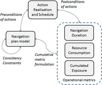
Operational users are not only interested in performance, feasibility or scalability, but at first in mission efficiency. In this paper, we consider maximizing mission observations while taking into account time, energetic or exposure constraints. To satisfy user needs, the problem must be addressed globally, which requires composition of different mathematical constraints. This can be done using a declarative logical approach, constraint predicates and classical operators (Hentenryck et al., Reference Hentenryck, Saraswat and Deville1998). Due to the introduction of complex navigation constraints related to actions description, other approaches cannot be used in a straightforward way. The Figure 3 describes the different constraint-based models that express the complete problem. Each model describes a piece of the solution space and comprises a set of variables with basic applicative constraints. Models are related with constraints in order to provide consistent solutions. Five models represent the problem formulation:
-
∙ Navigation plan, as a sequence of navigation way points that compose a consistent flight plan.
-
∙ Actions realization and scheduling, that are defined thanks to post and preconditions, as well as execution dates.
-
∙ Operational metric models, which are elaborated for resource consumption, UAV exposure and flight duration. These constraints result from cumulated variables over the flight path.
Problem formulation using multiple constraint models

The search algorithm described in the sequel, strongly rely on this model-based representation. Search techniques can be complex to design (in the case of A*) or models difficult to express (in the case of LP). Furthermore, as shown in previous works, the problem can be extended in several ways by combining different formulations. Search algorithms and heuristics must be developed or adapted without reconsidering the whole model. This can be achieved using CLP expressiveness, under a model-based development approach. CLP is a competitive approach to solve either constrained path or scheduling problems. In CLP, CSP follows a declarative formulation and is decoupled from search algorithms, so that both of them can be worked out independently. Designers can perform a late binding between CSP formulation and search algorithm. This way, different search techniques can be evaluated over multiple problem formulations. The development method also enables an easier management of tool evolutions by the designers. CSP formulation and search algorithms are implemented with the CLP(FD) domain of SICStus Prolog library. It uses the state-of-the-art in discrete constrained optimization techniques: Arc Consistency-5 (AC-5) for constraint propagation, using CLP(FD) predicates. With AC-5, variable domains get reduced until a fixed point is reached by constraint propagation.
Most of constraint programming frameworks have different tools to design hybrid search techniques, by integrating Metaheuristics, OR and LP algorithms (Ajili & Wallace, Reference Ajili and Wallace2004). An hybrid approach is proposed to solve the mission planning problem by exploiting Dijkstra algorithm and to elaborate a meta-metric over search exploration structure. This approach, known as probing, relies on problem relaxation to deduce the search tree structure. This can be done either statically or dynamically. The CLP framework also enables concurrent solving over problem variables.
The global search technique under consideration guarantees completeness, solution optimality and proof of optimality. It relies on three main algorithmic components:
-
∙ Variable filtering with correct values, using specific labelling predicates to instantiate problem domain variables. AC being incomplete, value filtering guarantees the search completeness.
-
∙ Tree search with standard backtracking when variable instantiation fails.
-
∙ B&B for cost optimization, using minimize predicate.
Designing a good search technique consists in finding the right variables ordering and value filtering, accelerated by domain or generic heuristics. In general, these search techniques are implemented with a conjunction of multiple specific labelling predicates.
4 Problem formalization
A navigation plan is represented using a directed graph G(X, U) where
-
∙ the set U of edges represents possible paths;
-
∙ the set V of vertices are navigation points. In the remaining of the paper, a vertex is denoted x, while an edge can be denoted either u or (x, x′).
4.1 Navigation plan
A navigation plan is defined by the set of positive flows over edges. The set of variables φ u ∈{0, 1} models a possible path from start∈X to end∈X, where an edge u belongs to the navigation plan if and only if a decision variable φ u =1. The resulting navigation plan, can be represented as Φ={u|u∈U, φ u =1}.
4.2 Consistency constraints
From an initial position to a final one, path consistency is enforced by flow conservation equations, where ω +(x) ⊂ U and ω −(x) ⊂ U are outgoing and incoming edges from vertex x, respectively:
 $$\mathop{\sum}\limits_{u\,\in\,\omega ^{{\plus}} \left( {{\rm start}} \right)} {\varphi _{u} \,{\equals}\,1,} \,\mathop{\sum}\limits_{u\,\in\,\omega ^{{\minus}} \left( {{\rm end}} \right)} {\varphi _{u} \,{\equals}\,1} $$
 $$\mathop{\sum}\limits_{u\,\in\,\omega ^{{\plus}} \left( x \right)} {\varphi _{u} \,{\equals}} \mathop{\sum}\limits_{u\,\in\,\omega ^{{\minus}} \left( x \right)} {\varphi _{u} \,⩽\, 1} $$
Since flow variables are {0, 1}, equation (2) ensures path connectivity and uniqueness while equation (1) imposes limit conditions for starting and ending the path. This constraint provides a linear chain alternating flyby waypoint and navigation along the graph edges.
4.3 Operational metric formulations with cumulative constraints
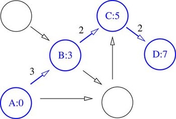
Assuming a given date D x associated with a position (e.g. vertex) x we use a path length formulation (3). Variable D x is expressing the time at which the UAV reaches a position x (see example in Figure 4). Assuming that variable d (x′, x) represents the time taken to perform the manoeuvre from position x′ to x (at an average edge speed) and perform potential observations on x′. This time cumulates action duration and navigation between waypoints.
Illustrating manoeuvres over a graph of navigation waypoints. This graph is a spatial representation of navigation plan. A solution, representing the unmanned aerial vehicle manoeuvres, corresponds to the set of positive values (here Φ={(A, B), (B, C), (C, D)}). Assuming a cumulative time metric (edge values are transit times), flyby instant is Δ={(A, 0), (B, 3), (C, 5), (D, 7)}

We have
 $$D_{x} \,{\equals}\mathop{\sum}\limits_{\left( {x',\,x} \right)\,\in\,\omega ^{{\minus}} \left( x \right)} {\varphi _{{\left( {x',\,x} \right)}} } \left( {d_{{\left( {x',\,x} \right)}} {\plus}D_{{x'}} } \right)$$
 $$\forall \left( {x,\,x'} \right)\in U,\,d_{{\left( {x,\,x'} \right)}} \in \Bbb{\tf="Macopen" N}, \,l_{{\left( {x,\,x'} \right)}} ⩽\,d_{{\left( {x,\,x'} \right)}} ⩽\, u_{{\left( {x,\,x'} \right)}} $$
Note that upper and lower speed limits (respectively u (x, x′) and l(x, x′)) in (4) are an edge. Other operational metrics are expressed with similar cumulative constraints. They are used to propagate resource consumption with variables <R x , r (x, x′)>, and UAV cumulated exposure with variables <E x , e (x, x′)>. These variables and constraints are also associated to vertices and edges as for constraint (4). In practice E x and R x are normalized as a percentage of consumption.
4.4 Action realization and schedule
The set of navigation points belonging to the plan P can also be expressed as follows:
 $$\forall x,\,n_{x} \,{\equals}\,{\rm min}\left( {1,\,D_{x} } \right),\,P\,{\equals}\,\left\{ {x\in X,\,n_{x} \,{\equals}\,1} \right\}$$
where n x states whether a position x is part of the navigation plan. If D x =0, the UAV does not flyby x. For simplicity, n x is assimilated to a Boolean variable.
A set of potential observation actions O is represented by ||V|| variables O x ∈{0, 1} and
-
∙ an observation duration constant δ x .
-
∙ a resource consumption constant ρ x .
-
∙ a visibility exposure constant η x .
If there is no action on vertex O x to be performed, its default value is 0. Action activation model is defined using the following preconditions (6) and postconditions (7–9):
 $$\eqalignno{ O_{x} & ⇒n_{x} \wedge{\rm E}_{x} \,⩾\, v_{x} \cr & \forall x,\,\forall x'\in\omega ^{{\plus}} \left( x \right) $$
 $$d_{{\left( {x,\,x'} \right)}} \,{\equals}\,\delta _{{\left( {x,x'} \right)}} {\plus}O_{x} .\delta _{x} $$
 $$r_{{\left( {x,\,x'} \right)}} \,{\equals}\,\rho _{{\left( {x,\,x'} \right)}} {\plus}O_{x} .\rho _{x} $$
 $$e_{{\left( {x,\,x'} \right)}} \,{\equals}\,\eta _{{\left( {x,\,x'} \right)}} {\plus}O_{x} .\eta _{x} $$
and where constant δ(x, x′) is the time to navigate from point x to x′.
In equation (6), the constant v x is an exposure threshold that is tolerated and compared with the total exposure up to waypoint x. Indeed, to satisfy the action, the UAV must be incoming to the observation location, which is the role of the term n x . This way, each observation precondition is constrained by the level of exposure. The observation resulting schedule can be defined by the waypoint flyby dates D x .
In this paper, arrival date at the recovery point is enough to constraint the whole CSP. However, the model can be extended to express preconditions for energy and time on observation activations.
D end⩽D max, where D max is the maximal mission duration.
Similarly, there must be remaining energy when arriving at the recovery point.
E end⩾0.
Other preconditions can be defined, depending on the type of action to perform (including time windows, communication, target mobility). Using our model, it is easy to overload the conjunction. However, the problem can become very complex and there is not necessarily a need as long as we consider a unique UAV. Moreover, we notice that the set of preconditions is predominant compared with postconditions.
4.5 Optimization problem
The final cost function is the total amount of observations to perform.
 $$\Omega \left( V \right)\,{\equals}\,\mathop{\sum}\limits_{x\,\in \,V} {O_{x} } $$
The sets of decision variables are Φ and O such that the CSP can then be formulated in Prolog as follows (1):

5 Search algorithms
5.1 Overview
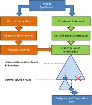
The goal of hybridizing global solving with stochastic approaches is to save the number of backtracks by quickly focussing the search towards good solutions. It consists in designing the tree search according to the problem structure, revealed by the probe. The idea is to use the prober to order problem variables, as a pre-processing. Instead of dynamic probing with tentative values such as in (Sakkout & Wallace, Reference Sakkout and Wallace2000), this search strategy uses a static prober which orders problem variables to explore according to the relaxed solution properties. Then, the solving follows a standard CLP search strategy, combining variable filtering, AC-5 and B&B. As shown in Figure 5, the probing technique proceeds in three steps (the three blocks on the left). The first one is to establish the solution to the relaxed problem. As a reference, we can, for example, compute the shortest path between starting and ending vertices, abstracting away mandatory waypoints. The next step is to establish a minimal distance between any problem variable and the solution to the relaxed problem. This step can be formally described as follows. Let X s ⊂ X be the set of vertices that belong to the relaxed solution. The distance is given by the following evaluation:
 $$\forall x\in X,\,\delta \left( x \right)\,{\equals}\,\mathop{{{\rm min}}}\limits_{{x'\,\in \,X_{s} }} \left| {\left| {\left( {x,\,x'} \right)} \right|} \right|$$
where ||.|| is a specific distance metric (in our case, the number of vertices between x and x′). The last step uses the resulting partial order to sort problem variables in ascending order. At global solving level the relaxed solution is useless, but problem variables are explored following this order.
Diagram of the complete solver using probing techniques

5.2 Properties
Two interesting probe properties can be highlighted:
-
∙ probe complexity: since computation of minimum distance between a vertex and any node is polynomial thanks to Dijkstra or Bellman-Ford algorithms, the resulting probe construction complexity is still polynomial in worst cases. The complexity of quicksort can in practice be neglected (see below for further details).
-
∙ probe completeness: since the probe does not remove any value from variable domains and the set of problem variables remains unchanged, the probe still guarantees global solving completeness.
Complexity analysis: let γ be the cardinality of V s and n the one of V. The complexity of probe construction is
-
∙ in worst case performance: O(n 2);
-
∙ in average case performance: O(γ.n.log(n)).
Sketch of the proof: the probing method first determines the minimal distance between all vertices X′∈X′ where X′=X\X s and any vertex x s ∈X s . A Dijkstra algorithm runs over a vertex x s allows to compute the distance to any point of X′ with O(n.log(n)) worst case complexity where n is the number of nodes in X. This has to be run over each vertex of X s and a comparison with previous computed values must be done for every vertex x′, to keep the lowest one. Thus, the resulting complexity is O(γ.n.log(n)). Variables must finally be sorted with a quicksort-like algorithm. The worst case complexity of this sort is O(n 2), but is generally computed in O(n.log(n)) (average case performance). Hence, the worst case complexity of the probing method is O(n 2), but in practice behaves in max{O(γ.n.log(n)), O(n.log(n))}=O(γ.n.log(n)).
5.3 Pseudocode
Algorithm 2 synthesizes probe construction mechanisms. First, a vector L d of size n (n being the number of nodes in X) is created and initialized with infinite values. At the end of the execution, it will contain a value associated to each vertex, corresponding to the minimal distance between this vertex and the solution to the relaxed problem. To do so, a Dijkstra algorithm is run over each node of the solution. During a run, distances are evaluated and replaced in L d if lower than the existing value (in the pseudo code, comparison are made at the end of a run for easier explanation). Once minimal distances are all computed, they are used to rank the set of vertices X in ascending order (to be used by the complete solver).

6 Preliminary results
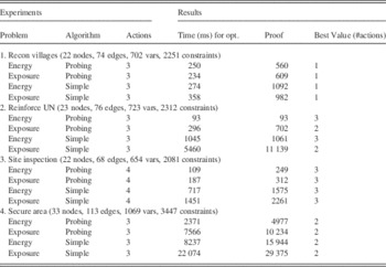
Experiments on four benchmarks are presented. They are representative of modern peace keeping missions or disaster relief. Missions must be executed in <30 minutes. Areas range from 5×5 to 20×20 km:
-
1. Recon villages: observing different villages after a water flooding event.
-
2. Reinforce UN: bring support to a United Nations mission by observing an unsecure town.
-
3. Sites inspections: observing different parts of a town during inspection of suspect sites.
-
4. Secure humanitarian area: observing different threats before securing refugees, over a large area.
For each benchmark, four experimentations are run. Two sets of runs are performed, one with the simple branch and bound, the other one with the probing method. For each set, two different constraints are preconditions to observation actions cumulated energetic resource and cumulated UAV exposure as defined by the generic constraint (3). In practice, the exposure threshold is set between 10 and 20% for each observation action. This overconstrains the problem, allowing us to observe performance differences.
Table 1 reports the time to find the optimal solution, as well as for proving optimality. It also shows the maximal number of observations that can be executed. Simple problems can be solved fairly quickly, but the last benchmark is more computation demanding, which is certainly due to a large area to cover. On the second benchmark, exposure constraints prevent from performing all observations. Again for all the problem instances, the probing method improves drastically the solver performances, which confirm former researches (Lucas et al., Reference Lucas, Guettier, Siarry, de La Fortelle and Milcent2010; Lucas & Guettier, Reference Lucas and Guettier2012). By comparing with energetic constraints, exposure preconditions makes the problem really harder to solve.
Results overview on benchmark scenarios, maximizing the number of action to perform

7 Conclusion
This paper shows the development of the mission planning framework, that can be used either for C2 systems or for unmanned systems. Introducing actions with complex preconditions and postconditions increases the practical complexity of problem instances. In particular, with the existing design, the solving approach does not scale huge numbers of observation or large graph structures. Nevertheless, as expected by previous results, the probing approach improves drastically solving performances. Using the modeling approach, the formulation of action preconditions and postconditions can be extended in several ways. Further works will focus on scalability as well as different forms of probing, relying on action definition in the relaxation process.
Acknowledgement
We acknowledge Pr. Arnaud de la Fortelle and Pr. Patrick Siarry for their constant support.