




1. Introduction
Fourier multipliers with operator-valued symbols have found many applications in the theory of abstract evolution equations, in particular, in connection with solvability (well-posedness) and regularity of integro-differential equations. A large class of such equations can be modelled by the following abstract, degenerate second-order problem with a convolution term:
 \begin{equation}
(P u')' + B u' + A u + c \ast u = f. \end{equation}
Here, A, B, P denote closed linear operators on a Banach space X and c is an operator-valued function.
For particular forms of (AP), the studies of their well-posedness on diverse vector-valued function spaces have been increased with occurring two seminal articles by Amann [Reference Amann2] and Weis [Reference Weis69], where operator-valued counterparts of classical multiplier theorems for Besov and Lebesgue–Bochner spaces on  $\mathbb{R}$ are provided. Those results indicated a right form of multiplier conditions (see [Reference Clément and Prüss31], [Reference Clément, de Pagter, Sukochev and Witvliet30]), which have been further adapted to different situations; see, e.g., periodic multiplier results in [Reference Arendt and Bu7, Reference Arendt and Bu8, Reference Strkalj and Weis68], which are relevant to this article.
In the literature, one can extract two lines of research corresponding to such studies: namely, when (AP) is considered in the Euclidean setting, that is, on  $\mathbb{R}$ or
 $\mathbb{R}_+$, and in the periodic one, that is, on
 ${\mathbb{T}}:=\mathbb{R}/\mathbb{Z}$ (i.e., when the periodic conditions are imposed). Each of these lines is represented by a long series of articles; to mention a few representative results, see for the first one, e.g., [Reference Amann2, Reference Aparicio and Keyantuo4–Reference Arendt, Batty and Bu6, Reference Auscher and Axelsson11, Reference Chill and Fiorenza27, Reference Chill and Srivastava29, Reference Król53, Reference Prüss and Simonett61, Reference Weis69], and for the second one, e.g., [Reference Arendt and Bu7, Reference Arendt and Bu8, Reference Bu and Cai19–Reference Bu and Fang23, Reference Fu and Li38, Reference Henríquez and Lizama41, Reference Keyantuo and Lizama49, Reference Keyantuo, Lizama and Poblete51, Reference Lizama55, Reference Lizama and Poblete56, Reference Lizama and Ponce58, Reference Poblete59] (as well as the references therein). Such studies correspond to the well-known research program formulated by Amman in [Reference Amann1, Section 3] and labelled as ‘pairs of maximal regularity’. In both settings, the basic idea for such studies is the same and relies on multiplier theorems. Roughly, by the theory of vector-valued distributions, the well-posedness and regularity questions for (AP) reduce to checking if corresponding Fourier multipliers with operator-valued symbols are bounded in a space under consideration. Such Fourier multiplier operators arise naturally via the representation formula for corresponding solution operators associated to a given form of (AP).
In the Euclidean setting, the so-called phenomenon of the extrapolation of  $L^p$-maximal regularity, which can be simply considered as a special variant of the well-posedness with respect to various Banach function spaces, have been studied recently; see, e.g., [Reference Auscher and Axelsson11, Reference Chill and Fiorenza27, Reference Chill and Król28, Reference Fackler, Hytönen and Lindemulder37, Reference Król53, Reference Prüss and Simonett61]. Beyond a natural theoretical interest in this phenomenon, the maximal regularity with respect to a more general function space is an important tool for the study of associated non-linear problems; see, e.g., [Reference Auscher and Axelsson11, Reference Kunstmann, Weis, Iannelli, Nagel and Piazzera54, Reference Prüss and Simonett62].
In the periodic case, the well-posedness and maximal regularity were mainly addressed in the context of the classical Lebesgue, Besov, Triebel–Lizorkin spaces; see the corresponding series of the references mentioned above. One of the aims of this article is to extend such results to a much wider context of general Banach function spaces and clarify the phenomenon of the extrapolation of Lp-maximal regularity for several periodic evolution equations modelled by (AP); see the main results of this article; theorems 6.5, 6.7, 6.9, and 6.12, as well as §7. These results, in particular, provide a periodic counterpart of the aforementioned line of research obtained in the Euclidean context.
The presented extension is not merely a consideration of more general function spaces. Even in the case of the classical spaces, our results have a new and noteworthy implication to the solvability of (AP) (and its particular forms). Generally, we provide a convenient framework which allows to handle various questions on the solvability of (AP) (such as the distributional and strong solvability, or maximal regularity estimates) in a unified manner. Moreover, our approach reveals an underlying structure of such studies, allows to simplify and unify technicalities mainly resulting from the fact that, in the context of some function spaces, one has to deal with higher order Marcinkiewicz’s conditions. This approach is based on theorem 6.2 (with lemma 6.4) and Fourier multiplier results, theorems 5.3 and 5.5. All these results may be of independent interest in the context of the general theory of abstract evolution equations and the theory of periodic Fourier multipliers.
More precisely, for instance, in theorem 6.2, we propose a new type of the joint multiplier condition involving the convolutor c and the multiplier symbol of a solution operator of (AP). This condition seems to be fundamental in the study of many particular forms of (AP) as we illustrate via the results of §6 and 7 mentioned above and by comparing them with known results from the literature. Furthermore, theorem 6.2 plainly shows how the structure of (AP) affects the relation between the regularity of the symbols of Fourier multipliers, which are involved in the study of (AP). Such an effect was somehow hidden in previous known results. Here, we point out that our theorem 6.2 applies to the most general form of (AP) (with no restriction on the domains of involved operators) and different types of multiplier conditions. This result and its proof should be confronted with the corresponding arguments in the existing line of research from the literature.
Our main Fourier multiplier results, theorems 5.3 and 5.5 show that the standard multiplier conditions, which in the literature are usually imposed on the symbol of a Fourier multiplier to get its boundedness on the classical (vector-valued) Lebesgue, Besov, or Triebel–Lizorkin spaces, are sufficient for its boundedness on much larger classes of spaces. Such classes include general Banach function spaces Φ and/or the scales of Besov and Triebel–Lizorkin spaces defined on the basis of Φ.
A deep analysis and subtle adaptation of many harmonic analysis tools were needed in order to get theorems 5.3 and 5.5. Some preparatory results obtained on the way to these results are new and may be of independent interest.
In particular, theorems 5.3 and 5.5 extend [Reference Arendt and Bu7, Theorem 1.3], [Reference Arendt and Bu8, Theorem 4.5], and [Reference Bu and Kim24, Theorem 3.2]. Our proofs differ from the proofs presented in those articles. We rely on direct maximal function estimates; see the proofs of lemma 2.2 and theorem 5.3. Regarding the strategy of the proof of our abstract extrapolation result, theorem 5.5, since the theory of periodic distributions presents a simplification in comparison to that on the real line, one could expect the same in the context of multiplier theorems. In fact, we show that such simplification is reflected mainly in the representation formulas for periodic Fourier multipliers; see §3.1 for the further comments and lemma 5.1. However, at some points (for instance, when the interplay between the regularity of the symbol and its Fourier transform is crucial), the Euclidean setting presents some benefits in comparison to the periodic one; cf. lemma 2.2. For this reason, instead of trying to prove some periodic results in a complete analogy to corresponding ones known in the Euclidean setting, we deduce them from their Euclidean counterparts via transference techniques; see the proof of theorem 5.5. The tools for such transference methods are worked out in §4 and may be of independent interest; see operator-valued variants of Jodeit’s type theorem, theorems 4.1 and 4.4, as well as lemmas 4.6 and 4.8.
2. Auxiliary results
2.1. Function spaces
We refer the reader to the monograph by Bennett and Sharpley [Reference Bennett and Sharpley14] for the background on Banach function spaces. Here, we mention only several facts we use in the sequel.
Let Ψ be a Banach function space over  $(G,\mathrm{d} t)$, where G denotes
 $\mathbb{R}$ or
 ${\mathbb{T}}$ equipped with the Lebesgue measure. It means that Ψ is a Banach space, which is an order ideal of
 $L^0:=L^0(G, \mathrm{d} t)$, i.e., for every
 $f\in L^0$ and
 $g\in \Psi$ if
 $|f|\leq |g|$, then
 $f\in \Psi$ and
 $\|f\|_\Psi \leq \|g\|_\Psi$. Here, L 0 stands for the space of all complex measurable functions on G (as usual, any two functions equal almost everywhere are identified). Moreover, Ψ has Fatou’s property, and by the Lorentz–Luxemburg theorem [Reference Bennett and Sharpley14, Theorem 2.7, p. 10],
 $(\Psi')' = \Psi$ with equal norms. Here,
 $\Psi'$ denotes the (Köthe) dual (or associated space) of Ψ; see [Reference Bennett and Sharpley14].
We define the vector-valued variant of Banach function spaces Ψ as follows. Let X be a Banach space with norm  $|\cdot|_X$. Set
 \begin{equation*}
\Psi (G; {X} ) :=\{f:G \rightarrow X \textrm{ strongly measurable}: \;\; |f|_X\in \Psi\}
\end{equation*}
and  $\|f\|_{\Psi(G;X)} : = \||f|_X\|_{\Psi}$ for
 $f\in \Psi (X)$. Throughout, the symbol Φ is reserved to denote a Banach function space over
 $({\mathbb{T}},\mathrm{d} t)$. Note that if a function
 $e_0(\tau):= 1$
 $(\tau \in {\mathbb{T}})$ is in Φ, then by the ideal property of Φ we get that
 $L^\infty({\mathbb{T}};X)\subset \Phi({\mathbb{T}}; X)=:\Phi(X)$. In particular, if
 ${\mathcal P}({\mathbb{T}};X)$ denotes the set of all X-valued polynomials on
 ${\mathbb{T}}$, i.e.,
 \begin{equation*}
{\mathcal P}(X):={\mathcal P}({\mathbb{T}};X):= \left\{\sum_{k=-N}^{N} e_k \otimes x_k: N\in \mathbb{N}, x_k\in X \right\}
\end{equation*}
then  ${\mathcal P}(X)\subset \Phi(X)$. Here,
 $(e_k \otimes x)(\tau):= e_k(\tau) x$, where
 $e_k (\tau):= \tau^k$ (
 $\tau\in {\mathbb{T}}$,
 $k\in \mathbb{Z}$,
 $x\in X$).
Moreover, we introduce a variant of vector-valued Besov and Triebel–Lizorkin spaces corresponding to a Banach function space Φ.
Let  ${\mathcal D}'({\mathbb{T}}; X):= {\mathcal L}({\mathcal D},X)$, where
 ${\mathcal D}:={\mathcal D}({\mathbb{T}})$ is the space of all complex-valued infinitely differentiable functions on
 ${\mathbb{T}}$ equipped in the usual locally convex topology. We refer to [Reference Schmeisser and Triebel66, Section 3] or [Reference Edwards35] for the backgrounds on the scalar distributions on
 ${\mathbb{T}}$ and to [Reference Arendt and Bu8, Section 2] for their vector-valued counterpart. For instance, relying on [Reference Arendt and Bu8, Proposition 2.1], it is readily seen that for each
 $\psi\in {\mathcal C}(\mathbb{R})$ with the compact support, the operator
 $\psi(\Delta)$ given by
 \begin{equation*}
\psi(\Delta)f := \sum_{k\in\mathbb{Z}} e_k\otimes \psi(k) \hat f(k) \qquad (f\in {\mathcal D}'({\mathbb{T}}; X))
\end{equation*}
is in  ${\mathcal L}({\mathcal D}'({\mathbb{T}}; X))$.
Let  $\{\psi_j\}_{j \in \mathbb{N}_0}$ be the resolution of the identity on
 $\mathbb{R}$ generated by a function
 $\psi\in {\mathcal C}^\infty(\mathbb{R})$ such that
 $\psi\equiv 1$ on
 $[-1,1]$ and
 ${\operatorname{supp}} \psi \subset [-2,2]$, i.e.,
 \begin{equation*}
\psi_0 :=\psi, \qquad \psi_j := \psi(2^{-j} \cdot) - \psi(2^{-j+1} \cdot)\quad \textrm{for } j\in \mathbb{N}.
\end{equation*}
One can check that  $\{\psi_j(\Delta)\}_{j\in \mathbb{N}_0}$ is the resolution of the identity operator on
 ${\mathcal D}'({\mathbb{T}};X)$, i.e., for every
 $f\in {\mathcal D}'({\mathbb{T}}; X)$
 \begin{equation*}
\sum_{j\leq N} \psi_j(\Delta)f = \psi(2^{-N} \Delta)f \rightarrow f \qquad \textrm{in } {\mathcal D}'({\mathbb{T}};X)\ \textrm{as } N\rightarrow \infty.
\end{equation*}
Let Φ be a Banach function space over  $({\mathbb{T}}, \mathrm{d} t)$. For all
 $s\in \mathbb{R}$ and
 $q\in [1,\infty]$, we set (with usual modification when
 $q=\infty$):
 \begin{align*}
& B^{s,q}_{\Phi}({\mathbb{T}}, X)\\ &\quad := \left\{f\in {\mathcal D}'({\mathbb{T}}; X):\,\, \|f\|_{B^{s,q}_{\Phi}({\mathbb{T}}, X)} :=\left( \sum_{j=0}^\infty \| 2^{sj} \psi_j(\Delta) f \|^q_{\Phi({\mathbb{T}}; X)} \right)^{1/q} \lt \infty\right\},
\end{align*}
 \begin{equation*}
F^{s,q}_{\Phi}({\mathbb{T}},X) := \left\{f\,{\in}\, {\mathcal D}'({\mathbb{T}}; X): \|f\|_{F^{s,q}_{\Phi}({\mathbb{T}},X)} :=\left\| \!\left( \sum_{j=0}^\infty | 2^{sj} \psi_j(\Delta)f |^q_X \right)\!^{1/q} \right\|_\Phi\,{ \lt }\, \infty \right\}.
\end{equation*}
For  $G=\mathbb{R}$ and a general Banach function spaces Ψ over
 $(\mathbb{R},\mathrm{d} t)$, the corresponding generalized vector-valued Besov
 $B^{s,q}_\Psi(\mathbb{R}; X)$ and Triebel–Lizorkin spaces
 $F^{s,q}_\Psi(\mathbb{R},X)$ were introduced in [Reference Król53, Section 2]. In the case when
 $G={\mathbb{T}}$, the vector-valued counterpart of the classical Besov spaces
 $B^{s,q}_p({\mathbb{T}})$, i.e., for
 $\Phi=L^p$ over
 $({\mathbb{T}}, \mathrm{d} t)$, was introduced in [Reference Arendt and Bu8]. In the both cases (
 $G={\mathbb{T}}$ or
 $G=\mathbb{R}$), under some additional assumption on Ψ, one can show that the spaces
 $B^{s,q}_\Psi(G;X)$ and
 $F^{s,q}_\Psi(G;X)$ share most of the properties of their well-known scalar prototypes which correspond to
 $\Psi = L^p$ and
 $X = \mathbb{C}$. For our further purposes, we only need a few basic properties of the spaces
 $B^{s,q}_\Phi({\mathbb{T}}; X)$ and
 $F^{s,q}_\Phi({\mathbb{T}}; X)$ corresponding to a general Banach function space Φ over
 $({\mathbb{T}},\mathrm{d} t)$; see proposition 2.3. For their proofs, we need a preliminary result on the boundedness of Fourier multipliers
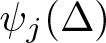 $\psi_j(\Delta)$,
 $j\in \mathbb{N}_0$, (and other ones) on the underlying space
 $\Phi(X)$. Then, the proof of proposition 2.3 can be carried out in an analogy to the non-periodic case when
 $G=\mathbb{R}$ as it has been treated in [Reference Król53]; see [Reference Król53, Lemma 3.6] and [Reference Król53, Lemma 5.3]. However, it should be pointed out that in a comparison to the proofs of some results in the case
 $G=\mathbb{R}$, the proofs of their periodic counterparts admit an essential simplification, which we indicate below; see also §3.1.
As it could be already noted above, we omit ‘ ${\mathbb{T}}$’ in the symbols of spaces over
 $({\mathbb{T}}, \mathrm{d} t)$. Similarly, in the scalar case, i.e., when
 $X=\mathbb{C}$,
 $\mathbb{C}$ is also omitted in the corresponding symbols. For instance,
 $B^{s,q}_\Phi(X)$ stands for
 $B^{s,q}_\Phi({\mathbb{T}};X)$ and
 ${\mathcal C}^\infty_c(\mathbb{R})$ denotes
 ${\mathcal C}^\infty_c(\mathbb{R};\mathbb{C})$, etc.
2.2. Preliminary results on boundedness of periodic multipliers
For a polynomially bounded sequence  $m:\mathbb{Z}\rightarrow {\mathcal L}(X,Y)$, we write
 $\check m$ to denote the corresponding periodic distribution in
 ${\mathcal D}'({\mathcal L}(X,Y))$, i.e.,
 \begin{equation*}
\check m := \sum_{k\in \mathbb{Z}} e_k\otimes m(k).
\end{equation*}
Lemma 2.1. Let  $m:\mathbb{Z} \rightarrow {\mathcal L}(X,Y)$ be such that
 $\check m$ is in
 $L^{\infty}({\mathcal L}(X,Y))$. Then, for every Banach function space Φ over
 $({\mathbb{T}},\mathrm{d} t)$ such that
 $L^\infty\subset \Phi \subset L^1$ the operator
 $m(\Delta)$ given by
 \begin{equation*}
m(\Delta)f := \sum_{k} e_k \otimes m(k) \hat f (k) \quad f\in {\mathcal D}'(X)
\end{equation*}
is in  ${\mathcal L}(\Phi(X),\Phi(Y))$ with
 $\|m(\Delta)\|_{{\mathcal L}(\Phi(X),\Phi(Y))}\leq c_\Phi \|\check{m}\|_{L^\infty}\|\chi_{\mathbb{T}}\|_\Phi$, where
 $c_\Phi$ denotes the norm of embedding operator from Φ into L1.
Proof. A standard argument shows that  $\Phi\hookrightarrow L^1$, i.e.,
 $\|g\|_{L^1}\leq c_{\Phi} \|g\|_\Phi$ (
 $g\in \Phi$). Since for every
 $\eta \in L^\infty$,
 $g\in \Phi$, and
 $\tau \in {\mathbb{T}}$, we have
 \begin{equation*}
| (\eta \ast g) (\tau)|\leq c_\Phi \|\eta\|_{L^\infty} \|g\|_\Phi
\end{equation*}
we infer that
 \begin{equation*}
\|\eta \ast g \|_\Phi\leq c_\Phi \|\eta\|_{L^\infty} \|
\chi_{\mathbb{T}}\|_\Phi \|g\|_{\Phi},
\end{equation*}
where  $\chi_{\mathbb{T}}$ is the characteristic function of
 ${\mathbb{T}}$. Since for every
 $f\in L^1(X)$, we have
 \begin{equation*}
| (m(\Delta)f) (\tau) |_Y = |(\check m \ast f) (\tau) |_Y \leq \big(\| \check m \|_{{\mathcal L}(X,Y)} \ast |f|_X\big) (\tau)\qquad (\tau \in {\mathbb{T}}),
\end{equation*}
the proof is complete.
In particular, lemma 2.1 shows that each operator  $\psi_j(\Delta)$,
 $j\in \mathbb{N}_0$, is bounded on
 $\Phi(X)$ if
 $L^\infty\subset \Phi \subset L^1$. To show their uniform boundedness on
 $\Phi(X)$, we need an additional assumption on the boundedness of the Hardy–Littlewood maximal operator on Φ.
Recall that the Hardy–Littlewood maximal operators  $M_{\mathbb{T}}$ and
 $M_{\mathbb{R}}$ are defined by
 \begin{equation*}
M_{\mathbb{T}} f(\tau) := \sup_{\epsilon \gt 0} \frac{1}{\epsilon}\int_{\Gamma(\tau, \epsilon)}
|f(\zeta) | \, |\mathrm{d} \zeta| \qquad (\tau \in {\mathbb{T}})
\end{equation*}
for  $f\in L^1({\mathbb{T}})$, where
 $\Gamma(\tau, \epsilon):= {\mathbb{T}}\cap \{z\in \mathbb{C}: |z-\tau| \leq \epsilon \}$, and
 \begin{equation*}
M_{\mathbb{R}} f(t) := \sup_{\epsilon \gt 0} \frac{1}{2\epsilon} \int_{[t-\epsilon, t+\epsilon]} |f(s)| \mathrm{d} s \qquad (t\in \mathbb{R})
\end{equation*}
for  $f\in L^1_{loc} (\mathbb{R})$. In the view of the standard identification between the function f on
 ${\mathbb{T}}$ with its 2π-periodic extension
 $\widetilde{f}$ on
 $\mathbb{R}$,
 $\widetilde{f}(t):=f(e^{it})$,
 $t\in\mathbb{R}$, there exists a constant c > 0 such that
 \begin{equation*}
c^{-1} (M_{\mathbb{R}}\widetilde{f})(t)\leq (M_{\mathbb{T}} f)(e^{it})\leq c (M_{\mathbb{R}}\widetilde{f})(t) \qquad (f\in L^1({\mathbb{T}}), t\in\mathbb{R}).
\end{equation*}
Note that the assumption that  $M_{\mathbb{T}}$ is bounded on a Banach function space Φ implies that
 $L^\infty\subset \Phi \subset L^1$. Indeed, if
 $f\in \Phi\setminus\{0\}$, then there exist a constant c > 0 and a measurable subset A of
 ${\mathbb{T}}$ such that
 $|f|\geq c\chi_A$, i.e.,
 $\chi_A\in \Phi$. Hence, by the boundedness of
 $M_{\mathbb{T}}$ on Φ, we get that
 $M_{\mathbb{T}} \chi_A \geq \frac{|A|}{2 \pi}$. Consequently, by the ideal property of Φ, we obtain that
 $L^\infty\subset \Phi$.
The following lemma provides a periodic counterpart of [Reference Stein67, Chapter 2, (17) p. 57]. For its proof, we need a vector-valued variant of Fejér’s theorem (see, e.g., [Reference Arendt and Bu7, Proposition 1.1]), which asserts that for an arbitrary Banach space X and  $g\in L^1({\mathbb{T}}; X)$, if
 $S_l(g):= \sum_{|k|\leq l} e_k\otimes \hat g(k)$ for
 $l\in \mathbb{N}_0$, then
 \begin{equation*}
\frac{1}{N+1} \sum_{l = 0}^{N} S_l(g)\rightarrow g \quad \textrm{as } N\rightarrow \infty\ \textrm{in } L^1({\mathbb{T}};X).
\end{equation*}
Lemma 2.2. (i) Let  $\eta \in {\mathcal C}_c(\mathbb{R}; {\mathcal L}(X,Y))$ be such that
 $\|{\mathcal F}^{-1}\eta(t)\|_{{\mathcal L}(X,Y)}\leq \phi(t)$,
 $t\in \mathbb{R}$, for an even, radially decreasing, integrable function ϕ on
 $\mathbb{R}$. Then, there exists a constant c > 0 such that for every
 $f\in L^1({\mathbb{T}}; X)$ we have
 \begin{equation}
|\eta(\Delta)f(\tau)|_{Y} \leq c \|\phi\|_{L^1(\mathbb{R})} (M_{\mathbb{T}} |f|_X)(\tau) \qquad (\tau \in {\mathbb{T}}).
\end{equation}
(ii) Let  $\eta \in {\mathcal C}_c^\infty(\mathbb{R})$ and set
 $\eta_\epsilon := \eta(\epsilon \cdot)$, ϵ > 0. Then, for every Banach function space Φ over
 $({\mathbb{T}},\mathrm{d} t)$ such that
 $M_{\mathbb{T}}$ is bounded on Φ, the operators
 $\eta_\epsilon(\Delta)$, ϵ > 0, are uniformly in
 ${\mathcal L}(\Phi(X))$.
Proof. (i) Let  $f\in L^1({\mathbb{T}};X)$. It is readily seen that for every
 $t\in \mathbb{R}$ the integral
 $\int_{\mathbb{R}} ({\mathcal F}^{-1}\eta)(s)\widetilde f(t-s) \mathrm{d} s =: ({\mathcal F}^{-1}\eta \ast \widetilde f) (t)$ is absolutely convergent. Suppose that
 ${\operatorname{supp}} \eta \subset [-K, K]$ for some
 $K \in \mathbb{N}$. Note that for every
 $t\in \mathbb{R}$ and l > K we have
 \begin{align*}
\eta(\Delta)f(e^{it}) & = \sum_{|k|\leq l} e^{itk} \int_{\mathbb{R}} e^{-isk} {\mathcal F}^{-1}\eta(s) \mathrm{d} s \hat f(k)\\
& = \int_{\mathbb{R}} {\mathcal F}^{-1} \eta(s) \sum_{|k|\leq l} e^{i(t-s)k} \hat f(k) \mathrm{d} s.
\end{align*}
Therefore, following the notation introduced in Fejér’s theorem, for N > K and  $t\in \mathbb{R}$, we get
 \begin{equation}
\frac{1}{N+1} \sum_{l=K}^{N}S_l(\eta(\Delta)f)(e^{it}) = \int_{\mathbb{R}} {\mathcal F}^{-1} \eta(s) \frac{1}{N+1} \sum_{l=K}^{N} S_l(g_t)(e^{i s}) \mathrm{d} s,
\end{equation}
where  $g_t(\tau):= f(e^{it}\bar \tau)$,
 $\tau\in {\mathbb{T}}$. By our assumption on
 ${\mathcal F}^{-1}\eta$, it is straightforward to show that the right-hand side of (2) converges to
 $({\mathcal F}^{-1}\eta \ast \widetilde f) (t)$ as
 $N\rightarrow \infty$. Since the left-hand side is equal
 $\frac{N-K+1}{N}\eta(\Delta)f(e^{it})$, we infer that for every
 $t\in \mathbb{R}$
 \begin{equation*}
\left| \eta(\Delta)f(e^{it})\right|_Y = \left|({\mathcal F}^{-1}\eta \ast \widetilde f) (t) \right|_Y \leq (\phi \ast |\widetilde f|_X)(t).
\end{equation*}
Further, note that for each ϵ > 0 there exists a function  $\phi_\epsilon:= \sum_{j=0}^N c_j \chi_{B_j}$, where Bj denotes an interval with centre at 0 and
 $c_j \gt 0$, such that
 $0\leq \phi_\epsilon\leq \phi$,
 $\|\phi - \phi_\epsilon\|_{L^\infty} \lt \epsilon$ and
 $\|\phi - \phi_\epsilon\|_{L^1} \lt \epsilon$. One can readily check that for every δ > 0 there exists ϵ such that for every
 $t\in \mathbb{R}$ we have
 \begin{equation*}
|(\phi\ast |\widetilde f|_X) (t)| \leq ((\phi - \phi_\epsilon) \ast |\widetilde f|_X) (t) + (\phi_\epsilon \ast |\widetilde f|_X) (t) \leq \delta + \|\phi_\epsilon\|_{L^1} (M_{\mathbb{R}} |\widetilde f|_X) (t).
\end{equation*}
Since there exists c > 0, independent of  $f\in L^1({\mathbb{T}};X)$, such that
 $(M_{\mathbb{R}}|\widetilde f|_X)(t)\leq c (M_{\mathbb{T}} |f|_X)(e^{it})$ for every
 $t\in \mathbb{R}$, we get (1).
(ii) Note that  $({\mathcal F}^{-1}\eta_\epsilon)(t) = \frac{1}{\epsilon}({\mathcal F}^{-1}\eta) (\frac{t}{\epsilon})$ for every ϵ > 0 and
 $t\in \mathbb{R}$. Moreover, there exists a constant C > 0 such that
 $|({\mathcal F}^{-1}\eta) (t)|\leq \frac{C}{1+t^2}$, which yields
 $|({\mathcal F}^{-1}\eta_\epsilon) (t)|\leq \frac{\epsilon^{-1} C}{1+(\epsilon^{-1}t)^2}=:\phi_\epsilon(t)$ for every
 $t\in \mathbb{R}$ and ϵ > 0. Since
 $\|\phi_\epsilon\|_{L^1} = C\pi$ for every ϵ. Therefore, (1) gives the desired claim.
2.3. Fundamental properties of generalized Besov and Triebel–Lizorkin spaces
Here, we collect the fundamental properties of such spaces, which play a role in our further studies; see proposition 2.3.
We start with some preliminaries. Note that for every  $s\in \mathbb{R}$ the space
 $B^{-s,1}_{\Phi'}(X^*)$ can be identified with a subspace of
 $(B^{s,\infty}_\Phi(X))^*$. Indeed, this identification is given by the following duality pairing: for each
 $f \in B^{s,\infty}_{\Phi}(X)$ and
 $g\in B^{-s,1}_{\Phi'}(X^*)$, we set
 \begin{equation}
\langle g , f \rangle:= \sum_{j,l\in \mathbb{N}_0} \int_{{\mathbb{T}}} \langle \psi_l(\Delta)g(t) , \psi_j(\Delta)f(t) \rangle_{X^*,X} \mathrm{d} t.
\end{equation}
Note that
 \begin{equation*}
\langle g , f \rangle = \sum_{j\in \{\pm 1, 0\}} \sum_{l\in \mathbb{N}_0}
\langle \breve{\psi}_{j}(\Delta)\psi_l(\Delta)g , \chi_j(\Delta)f \rangle_{\Phi'(X^*),\Phi(X)},
\end{equation*}
where  $\breve{\psi}_j:=\psi_j(-\cdot)$ and
 $\chi_j:=\psi_{j-1}+\psi_j+\psi_{j+1}$
 $(j\in \mathbb{N}_0)$ with
 $\psi_{-1} \equiv 0$ if j = 0.
Proposition 2.3. Let X be a Banach space and Φ be a Banach function space over  $({\mathbb{T}}, \mathrm{d} t)$. Let
 $s \in \mathbb{R}$ and
 $q \in [1,\infty]$. Then, the following assertions hold.
(i) If
 $L^\infty \subset \Phi\subset L^1$, then for
$
\mathbb{E} \in \left\{B^{s,q}_\Phi,\, F^{s,q}_\Phi \right\}$
(4)\begin{equation}
{\mathcal P}(X) \subset \mathbb{E}( X) \hookrightarrow {\mathcal D}'(X).
\end{equation}
In particular,
$\mathbb{E}(X)$ is a Banach space.(ii) If
$M_{\mathbb{T}}$ is bounded on Φ, then
${\mathcal P}(X)$ is a dense subset of
$B^{s,q}_\Phi(X)$ in the norm topology if
$q\in[1,\infty)$, and in the
$B^{-s,1}_{\Phi'}(X^*)$-topology of
$B^{s,\infty}_{\Phi}(X)$ if
$q=\infty$.More precisely, for every
$f\in B^{s,q}_\Phi(X)$, we have that
\begin{equation*}
\sum_{0\leq j\leq N} \psi_j(\Delta) f = \psi(2^{-N} \Delta)f \rightarrow f \quad \textrm{as } N\rightarrow \infty
\end{equation*}in
$B^{s,q}_\Phi(X)$ for each
$q \lt \infty$, and in the other case, i.e.,
$q=\infty$, the convergence holds in the
$\sigma(B^{s,\infty}_{\Phi}(X), B^{-s,1}_{\Phi'}(X^*))$-topology.(ii’) If
$M_{\mathbb{T}}$ is bounded on Φ and its dual
$\Phi'$, then for every
$q \in (1,\infty)$, the set of X-valued polynomials
${\mathcal P}(X)$ is a dense subset of
$F^{s,q}_\Phi(X)$ and for every
$f\in F^{s,q}_\Phi(X)$ we have that
\begin{equation*}
\sum_{0\leq j\leq N} \psi_j(\Delta) f = \psi(2^{-N} \Delta)f \rightarrow f \quad \textrm{as } N\rightarrow \infty.
\end{equation*}(iii) If
$M_{\mathbb{T}}$ is bounded on Φ, then for every distribution
$f\in {\mathcal D}'(X)$, f belongs to
$B^{s,q}_{\Phi}( X)$ if and only if
$\partial f$ belongs to
$B^{s-1,q}_\Phi(X)$. Moreover, the function
(5)\begin{equation}
B^{s,q}_\Phi( X) \ni f \mapsto \left\| \partial f \right \|_{B^{s-1,q}_\Phi(X)}
\end{equation}is an equivalent norm on
$B^{s,q}_\Phi( X)$.


Remark 2.4. (a) Compared to the case of the real line  $\mathbb{R}$ (see [Reference Król53, Lemma 3.6]), note that in the periodic case there is a common dense subset, i.e.,
 ${\mathcal P}(X)$, for all
 $\mathbb{E}(X)$ with
 \begin{equation*}
\mathbb{E} \in \{B^{s,q}_\Phi, \, F^{s,r}_\Phi\,: s\in \mathbb{R}, q\in [1,\infty], r\in (1,\infty) \}.
\end{equation*}
(b) In contrast to [Reference Król53, Lemma 3.6], in proposition 2.3, in the case of Besov spaces, we do not assume that  $M_{\mathbb{T}}$ is bounded on the dual of
 $\Phi'$.
By lemma 2.2, the proof of proposition 2.3 mimics that of the corresponding statements on  $\mathbb{R}$, [Reference Król53, Lemmas 3.6 and 5.4]. For the convenience of the reader, we provide some auxiliary observations which should be made.
The proof of proposition 2.3
(i) Since  ${\mathcal P} \subset L^\infty \subset \Phi$, the left inclusion in (4) holds readily. For the second one, note that since
 $ \Phi \hookrightarrow L^1$, we have
 $B^{s,q}_{\Phi}(X) \hookrightarrow B^{s,q}_1(X)$ and
 $F^{s,q}_{\Phi}(X)\hookrightarrow F^{s,q}_1(X)$. The continuity of the embeddings of the spaces
 $B^{s,q}_1(X)$ and
 $F^{s,q}_1(X)$ into
 ${\mathcal D}'(X)$ is a standard fact (see [Reference Schmeisser and Triebel66, Theorem 3.5.1, p. 162] for the scalar-valued case; cf. also [Reference Arendt and Bu8, Theorem 2.3] and [Reference Bu and Kim25, Proposition 2.3]).
(ii) Note that for every  $j\in \mathbb{N}$,
 $\psi_j(t)= \eta (2^{-j}t)$, where
 $\eta(t) :=\psi(t) - \psi(2t)$,
 $t\in \mathbb{R}$. Thus, by lemma 2.2(ii), the operators
 $\psi_j(\Delta)$,
 $j\in \mathbb{N}_0$, restrict to uniformly bounded operators in
 ${\mathcal L}(\Phi(X))$. Now the proof mimics the lines of the proof of the corresponding statement in [Reference Król53, Lemma 3.6]. Therefore, we omit it.
(ii’) Since  $F^{s,q}_{\Psi}(X) = B^{s,q}_\Psi(X)$ for every
 $\Psi=L^q_w$ with
 $q\in (1,\infty)$ and
 $w\in A_q({\mathbb{T}})$, by the point (ii), the statement
 $(ii^{\prime})$ holds for such spaces. The proof for a general Φ extrapolates from these particular ones via an adaptation of the Rubio de Francia iteration algorithm.
Let  ${\mathcal R}$ and
 ${\mathcal R}'$ denote the following sublinear, positive operators defined on Φ and
 $\Phi'$, respectively:
 \begin{equation}
{\mathcal R} g := \sum_{k=0}^\infty \frac{M_{\mathbb{T}}^k |g|}{(2\|M_{\mathbb{T}}\|_{\Phi})^k} \quad (g\in \Phi) \quad \textrm{and } \quad
{\mathcal R}' h := \sum_{k=0}^\infty \frac{M_{\mathbb{T}}^k |h|}{(2\|M_{\mathbb{T}}\|_{\Phi'})^k} \quad (h\in \Phi')
\end{equation}
Here,  $M_{\mathbb{T}}^k$ stands for the kth iteration of the Hardy–Littlewood operator
 $M_{\mathbb{T}}$,
 $M_{\mathbb{T}}^0 := I$, and
 $\|M_{\mathbb{T}}\|_\Phi := \sup_{\|g\|_\Phi \leq 1}\|M_{\mathbb{T}} g\|_{\Phi}$. Since
 \begin{equation*}
M({\mathcal R} g ) \leq 2 \|M\|_\Phi {\mathcal R} g \quad (g\in \Phi) \quad \textrm{and} \qquad M({\mathcal R}' h) \leq 2 \|M\|_{\Phi'} {\mathcal R} h \quad (h\in \Phi'),
\end{equation*}
for every  $g\in \Phi$ and
 $h\in \Phi'$ the functions
 ${\mathcal R} g$ and
 ${\mathcal R}'h$ belong to Muckenhoupt’s class
 $A_1({\mathbb{T}})$. Consequently, for every
 $q\in (1,\infty)$,
 $g\in \Phi$, g ≠ 0, and
 $h\in \Phi'$, h ≠ 0, the function
 \begin{equation}
w_{g,h,q}:=({\mathcal R} g)^{1-q} {\mathcal R}' h
\end{equation}
is in Muckenhoupt’s class  $A_q({\mathbb{T}})$ with the Aq-constant
 \begin{equation}
[w_{g,h,q}]_{A_q}\leq 2^q \|M\|_{\Phi}^{q-1} \|M\|_{\Phi'}.
\end{equation}
Moreover, note that if  $g\in \Phi(X)$, then
 $f\in L^q_w(X)$ for
 $w:= ({\mathcal R}|f|_X)^{1-q} {\mathcal R}'h$ with an arbitrary
 $h\in \Phi'$, h ≠ 0. Indeed, since
 $|g|_X\leq {\mathcal R}|g|_X$, we get
 \begin{equation*}
\int_{\mathbb{R}} |g|_X^q w \mathrm{d} t \leq \int_{\mathbb{R}} {\mathcal R}|g|_X {\mathcal R}' h \mathrm{d} t \leq \|{\mathcal R} |g|_X\|_\Phi \| {\mathcal R}'h\|_{\Phi'} \lt \infty.
\end{equation*}
By lemma 2.2 combined with Muckenhoupt’s theorem (see, e.g., [Reference Böttcher and Karlovich13]) we get that if
 \begin{equation*}
\mu_{w,q}: = \sup_{j\in \mathbb{N}_0} \|\psi_j(\Delta)\|_{{\mathcal L}(L^q_w(X))},
\end{equation*}
then  $\sup_{w\in {\mathcal W}} \mu_{w,q} \lt \infty$ for each
 ${\mathcal W}\subset A_q({\mathbb{T}})$ with
 $\sup_{w\in {\mathcal W}}[w]_{A_q} \lt \infty$.
Now we are in a position to apply Rubio de Francia’s extrapolation argument. Fix  $q\in (1,\infty)$. Let
 $f\in F^{s,q}_\Phi(X)$ and
 $f_N:= \sum_{j\leq N} \psi_j(\Delta)f$ for all
 $N\in \mathbb{N}$. Note that
 $f_N \in {\mathcal P}(X)$ and
 \begin{equation*}
\|f-f_N\|_{F^{s,q}_\Phi(X)} \lesssim \sum_{r=-1}^1 \Big\|\big( \sum_{j\geq N} 2^{jsq}|\psi_{j+r}(\Delta)\psi_j(\Delta)f|_X^q\big)^{1/q}\Big\|_{\Phi}.
\end{equation*}
For each  $r\in \{\pm 1, 0\}$ set
 \begin{equation*}
g_r:= g_{N,r,f} := \big( \sum_{j\geq N} 2^{jsq}|\psi_{j+r}(\Delta)\psi_j(\Delta)f|_X^q\big)^{1/q}, \quad \textrm{and}
\end{equation*}
 \begin{equation*}
g : = g_{N,f} := \big( \sum_{j\geq N} 2^{jsq}|\psi_j(\Delta)f|_X^q\big)^{1/q}\quad (N\in \mathbb{N}).
\end{equation*}
Let  $h\in \Phi'$ with h ≠ 0 and
 $w:= w_{g, h, q}= {\mathcal R}(g)^{1-q} {\mathcal R}' h$. Then,
 \begin{align*}
\mu_{w,q} \|{\mathcal R}\|_{{\mathcal L}(\Phi)} \|g\|_\Phi \|{\mathcal R}'\|_{{\mathcal L}(\Phi')} \| h\|_{\Phi'} & \geq \mu_{w,q} \|{\mathcal R} g\|_\Phi \|{\mathcal R}'h\|_{\Phi'} \\
& \geq \mu_{w,q} \left( \int_{\mathbb{T}} {\mathcal R} g {\mathcal R}' h \, \mathrm{d} t \right)^\frac{1}{q} \left( \int_{\mathbb{T}} {\mathcal R} g {\mathcal R}' h \, \mathrm{d} t \right)^\frac{1}{q'}\\
&\geq \left( \int_{\mathbb{T}} g_r^q w \,\mathrm{d} t \right)^\frac{1}{q} \left( \int_{\mathbb{T}} {\mathcal R} g {\mathcal R}' h \mathrm{d} t \right)^\frac{1}{q'}\\
&\geq \int_{\mathbb{T}} g_r {\mathcal R}' h \, \mathrm{d} t\\
&\geq \int_{\mathbb{T}} g_r |h| \, \mathrm{d} t.
\end{align*}
Since
 \begin{equation*}
\sup\left\{[w_{g_{N,f},h,q}]_{A_q}: f\in F^{s,q}_\Phi(X), N\in \mathbb{N}, h\in \Phi'\setminus \{0\} \right\} \lt \infty,
\end{equation*}
we get that
 \begin{equation*}
\mu: = \sup\left\{\mu_{w,q}: \, w=w_{g_{N,f}, h, q} \textrm{with } f\in F^{s,q}_\Phi(X), N\in \mathbb{N}, h\in \Phi'\setminus \{0\} \right\} \lt \infty.
\end{equation*}
Therefore, by the Lorentz–Luxemburg theorem, we infer that  $g_r \in \Phi(X)$ (
 $r\in \{\pm 1 ,0\})$ and for all
 $N\in \mathbb{N}$ we have
 \begin{equation*}
\| g_{N,r,f} \|_\Phi \leq \mu \|{\mathcal R}\|_{{\mathcal L}(\Phi)} \|{\mathcal R}'\|_{{\mathcal L}(\Phi')} \|f-f_N\|_\Phi.
\end{equation*}
Since, by Fatou’s property of Φ,  $f_N - f \rightarrow 0$ in
 $\Phi(X)$ as
 $N\rightarrow \infty$, we get the desired claim.
(iii) First note that for every  $f\in {\mathcal D}'(X)$ and
 $j\in \mathbb{N}_0$,
 $\partial f = \rho(\Delta) f$, where
 $\rho(t) = it$
 $(t\in\mathbb{R})$, and
 \begin{align*}
\|2^{(s-1)j} \psi_j(\Delta)\partial f\|_{\Phi(X)} & = \|2^{(s-1)j} (\rho\chi_j)(\Delta)\psi_j(\Delta)f\|_{\Phi(X)}\\
& \leq \|2^{-j} (\rho\chi_j)(\Delta)\|_{{\mathcal L}(\Phi(X))} \|2^{sj}\psi_{j}(\Delta)f\|_{\Phi(X)}.
\end{align*}
Moreover, if we set  $\eta(t):= t\psi(\frac{1}{2}t) - t\psi(4t)$
 $(t\in \mathbb{R})$, then for every
 $j\geq 2$ and
 $t\in \mathbb{R}$, we have
 \begin{equation*}
\eta (2^{-j}t) = -i 2^{-j}(\rho \chi_j)(t).
\end{equation*}
Thus, by lemma 2.2, we infer that  $\sup_{j\in \mathbb{N}_0} \|2^{-j} (\rho\chi_j)(\Delta)\|_{{\mathcal L}(\Phi(X))} \lt \infty$, and consequently
 $\partial f \in B^{s-1,q}_\Phi(X)$ if
 $f\in B^{s,q}_\Phi(X)$.
Now, suppose that  $f\in {\mathcal D}'(X)$ with
 $\partial f \in B^{s-1,q}_{\Phi}(X)$. Let
 $\eta(t) := \frac{1}{t} \psi(\frac{1}{2}t) - \frac{1}{t} \psi(4t)$. Then, for every
 $j\geq 2$, we have
 $2^j\chi_j(t) \frac{1}{\rho(t)} = -i \eta (2^{-j} t)$
 $(t\in \mathbb{R})$ and
 \begin{align*}
\|2^{sj}\psi_j(\Delta)f\|_{\Phi(X)} & \leq \| 2^{j} (\chi_j \frac{1}{\rho})(\Delta)\|_{{\mathcal L}(\Phi(X))} \| 2^{(s-1)j} \psi_j(\Delta) \rho(\Delta) f \|_{\Phi(X)} \\
& = \| \eta(2^{-j}\Delta)\|_{{\mathcal L}(\Phi(X))} \| 2^{(s-1)j} \psi_j(\Delta) \partial f \|_{\Phi(X)}.
\end{align*}
Therefore, lemma 2.2 shows that  $f\in B^{s,q}_{\Phi}(X)$. This completes the proof.
Remark 2.5. (a) The norms  $\|\cdot\|_{B^{s,q}_\Phi(X)}$(respectively,
 $\|\cdot\|_{F^{s,q}_\Phi(X)}$) of course depend on the chosen function ψ generating the resolution of the identity involved in the definition of the corresponding spaces
 $B^{s,q}_\Phi(X)$(respectively,
 ${F^{s,q}_\Phi}(X)$). However, the arguments presented in the proof of proposition 2.3(ii) (respectively (ii’)) show that the norms corresponding to different generating functions are equivalent when the Hardy–Littlewood maximal operator
 $M_{\mathbb{T}}$ is bounded on Φ (respectively, on Φ and its dual
 $\Phi'$). The fact that, in the case of Triebel–Lizorkin spaces, one cannot drop, in general, the boundedness of
 $M_{\mathbb{T}}$ on
 $\Phi'$ is well-known from the classical situation, i.e.,
 $\Phi= L^\infty$; cf. [40, Subsection 2.1.4]. (b) Straightforward arguments show that
 $B^{-s,1}_\Phi(X^*)$ is separating on
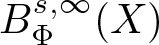 $B^{s,\infty}_{\Phi}(X)$ for every
 $s\in \mathbb{R}$. We apply it in §5.
3. Fourier multipliers
3.1. The representation formula for periodic multipliers
Let X and Y be Banach spaces. By the representation result for the periodic distributions  ${\mathcal D}'({\mathbb{T}};X)$ (see, e.g., [Reference Arendt and Bu8, Proposition 2.1], as well as [Reference Edwards34, Chapter 12] or [Reference Schmeisser and Triebel66, Section 3] for its scalar-valued prototype), it is easily seen that for an arbitrary sequence
 $m:\mathbb{Z} \mapsto {\mathcal L}(X,Y)$ with a polynomial growth, the following operator
 \begin{equation}
m(\Delta):{\mathcal D}'({\mathbb{T}},X) \ni f \mapsto \sum_{k\in \mathbb{Z}} e_k\otimes m(k)\hat f(k) \in {\mathcal D}'({\mathbb{T}}, Y)
\end{equation}
is well-defined and continuous (the series is convergent in  ${\mathcal D}'({\mathbb{T}}; Y)$).
Let Φ be a Banach function space over  $({\mathbb{T}},\mathrm{d} t)$ and
 \begin{equation*}
\mathbb{E} \in \{\Phi, B^{s,q}_\Phi, F^{s,r}_\Phi: s\in \mathbb{R}, q\in [1,\infty], r\in (1,\infty) \}.
\end{equation*}
A sequence  $m : \mathbb{Z} \to {\mathcal L}(X,Y)$ is called an
 $\mathbb{E}$-Fourier multiplier if
 $m(\Delta)$ restricts to an operator in
 ${\mathcal L}(\mathbb{E}({\mathbb{T}};X), \mathbb{E}({\mathbb{T}}; Y))$. We set
 ${\mathcal M}_{\mathbb{E}}({\mathbb{T}}; X,Y)$ to denote the space of all
 ${\mathcal L}(X,Y)$-valued
 $\mathbb{E}$-Fourier multipliers, and we simply write
 ${\mathcal M}_p({\mathbb{T}}; X,Y)$ for
 ${\mathcal M}_{L^p}({\mathbb{T}}; X,Y)$.
Now, let Ψ be a Banach function space over  $(\mathbb{R},\mathrm{d} t)$ and
 \begin{equation*}
\mathbb{E} \in \{\Psi, B^{s,q}_\Psi, F^{s,r}_\Psi: s\in \mathbb{R}, q\in [1,\infty], r\in (1,\infty) \}.
\end{equation*}
Let  $m : \mathbb{R} \to {\mathcal L}(X,Y)$ be a bounded measurable function and
 \begin{equation*}
D_m := \{f \in {\mathcal S}'(\mathbb{R}; X) : {\mathcal F} f \in L^1_{loc}(\mathbb{R}; X) \text{and } m(\cdot){\mathcal F} f \in {\mathcal S}'(\mathbb{R}; Y)\}
\end{equation*}
Then, m is called a  $\mathbb{E}$-Fourier multiplier, if the following operator
 \begin{equation*}
m(D): D_m \cap \mathbb{E}(\mathbb{R};X)\ni f \mapsto {\mathcal F}^{-1}( m(\cdot) {\mathcal F} f) \in {\mathcal S}'(\mathbb{R};Y)
\end{equation*}
extends to an operator in  ${\mathcal L}(\mathbb{E}(\mathbb{R};X), \mathbb{E}(\mathbb{R}; Y))$. Similarly to the periodic case, we set
 ${\mathcal M}_{\mathbb{E}}(\mathbb{R}; X,Y)$ to denote the space of all
 ${\mathcal L}(X,Y)$-valued
 $\mathbb{E}$-Fourier multipliers, and we simply write
 ${\mathcal M}_p(\mathbb{R}; X,Y)$ for
 ${\mathcal M}_{L^p}(\mathbb{R}; X,Y)$.
Remark 3.1. Note that in a contrast to the representation formulas for Fourier multipliers on the real line, each periodic multiplier has a (canonical) representation formula (cf. [Reference Król53, Section 4]). More precisely, since it is not obvious how to define, in general, the extension of the pointwise multiplication of a function  $m \in L^\infty (\mathbb{R}; {\mathcal L}(X,Y))$ with a distribution
 $f\in {\mathcal S}'(\mathbb{R}; X)$, only in special cases one can show that the operator
 \begin{equation*}
m(D): {\mathcal S}(\mathbb{R}; X)\ni f \mapsto {\mathcal F}^{-1}( m(\cdot) {\mathcal F} f) \in {\mathcal S}'(\mathbb{R};Y)
\end{equation*}
extends to a continuous operator on whole  ${\mathcal S}'(\mathbb{R}; X)$. For instance, recall that by means of Schwartz’ kernel theorem, such an extension exists for each
 $m\in {\mathcal O}_M(\mathbb{R}; {\mathcal L}(X,Y))$, that is, slowly increasing, smooth functions. In this case, we have a formal expression for such an extension given for all
 $f\in {\mathcal S}'(\mathbb{R};X)$ by
 \begin{equation*}
m(D)f = {\mathcal F}^{-1} \Theta(m, {\mathcal F} f),
\end{equation*}
where Θ is a hypocontinuous, bilinear map from  ${\mathcal O}_M(\mathbb{R}; {\mathcal L}(X,Y))\times {\mathcal S}'(\mathbb{R}; X)$ into
 ${\mathcal S}'(\mathbb{R}; Y)$; see, e.g., Amann [Reference Amann2, Theorem 2.1]. Consequently, compared to the case of the real line, the study of periodic integro-differential equations is conceptually more straightforward at this point (cf., e.g., the presentation of [Reference Król53, Proposition 4.2] with theorem 5.5, see also [Reference Hytönen and Weis45, Problems 3.2 and 3.3]).
3.2. The multiplier conditions
For the convenience of the reader, we recall the notion of Marcinkiewicz’s type conditions used in the next sections.
Let X and Y denote Banach spaces and  $\gamma \in \mathbb{N}$. We say that a function
 $m: \mathbb{R}\rightarrow {\mathcal L}(X,Y)$ satisfies the Marcinkiewicz condition of order γ (in short, the
 $\mathfrak{M}^\gamma$-condition), if
 $m\in{\mathcal C}^\gamma(\dot{\mathbb{R}}; {\mathcal L}(X,Y))$ and
 \begin{equation*}
[m]_{\mathfrak{M}^\gamma}:=\max_{l=0,\ldots,\gamma}\sup_{t\neq 0} \|t^l m^{(l)}(t)\|_{{\mathcal L}(X,Y)} \lt \infty \quad \quad {(\frak M^\gamma)}.
\end{equation*}
Then, we write  $m\in \mathfrak{M}^\gamma (\mathbb{R};{\mathcal L}(X,Y))$.
Furthermore, let  $\widetilde{\frak M}^\gamma(\mathbb{R};{\mathcal L}(X,Y))$ denote a subclass of
 ${\frak M}^\gamma(\mathbb{R};{\mathcal L}(X,Y))$, which consists symbols m such that
 \begin{equation*}
[m]_{\widetilde{\mathfrak{M}}^\gamma}:=\max_{l=0,\ldots,\gamma}\sup_{t\neq 0} \|(1+|t|)^l m^{(l)}(t)\|_{{\mathcal L}(X,Y)} \lt \infty \quad \quad {(\widetilde{\frak M}^\gamma)}
\end{equation*}
and  $m(0^+)=m(0^-)$ (equivalently, m has continuous extension at 0).
The discrete counterpart is defined analogously. Namely, a sequence  $m : \mathbb{Z} \to {\mathcal L}(X,Y)$ satisfies the
 $\mathfrak{M}^\gamma$-condition, if
 \begin{equation*}
[m]_{\mathfrak{M}^\gamma}:=\max_{l=0,\ldots,\gamma}\sup_{k\in \mathbb{Z}} \|k^l (\Delta^l m)(k)\|_{{\mathcal L}(X,Y)} \lt \infty,
\end{equation*}
where  $(\Delta^lm)(k) = \sum_{j=0}^{l} \binom{l}{j} (-1)^{l-j} m(k+j)$ for
 $l\in \mathbb{N}_0$. Similarly, we write
 $m \in \mathfrak{M}^\gamma (\mathbb{Z};{\mathcal L}(X,Y))$.
Furthermore, we say that  $m: \mathbb{Z} \rightarrow {\mathcal L}(X,Y)$ satisfies the variational Marcinkiewicz condition, if
 \begin{equation*}
[m]_{Var}:=\sup_{k\in \mathbb{Z}} \|m(k)\|_{{\mathcal L}(X,Y)} + \sup_{j\geq 0} \sum_{2^j \leq |k| \lt 2^{j+1}} \|m(k+1) - m(k)\|_{{\mathcal L}(X,Y)} \lt \infty.
\end{equation*}
Set  $Var(\mathbb{Z}; {\mathcal L}(X,Y))$ to denote the space of all sequences which satisfy the above condition. Note that
 $ \mathfrak{M}^1(\mathbb{Z}; {\mathcal L}(X,Y)) \subset Var(\mathbb{Z}; {\mathcal L}(X,Y)) $.
Finally, we say that  $m: \mathbb{Z} \to {\mathcal L}(X,Y)$ satisfies the
 $\mathfrak{M}^\gamma_{{\mathcal R}}$-condition and write
 $m\in \mathfrak{M}^\gamma_{\mathcal R}(\mathbb{Z}; {\mathcal L}(X,Y))$, if the sets
 $\{k^l\Delta^l m(k)\}$ are
 ${\mathcal R}$-bounded for all
 $l\in \{0,1,\ldots,\gamma\}$. We refer the reader, e.g., to [Reference Kunstmann, Weis, Iannelli, Nagel and Piazzera54] or [Reference Denk, Hieber and Prüss33], for the background on
 ${\mathcal R}$-boundedness.
4. Transference results
In this section, we provide some crucial ingredients of the results presented in the following sections. These ingredients allow to transfer directly some results known in the real-line setting to the periodic one, rather than rephrasing the proofs from  $\mathbb{R}$ to
 ${\mathbb{T}}$. Such transference methods reveal some natural questions, which maybe of independent interest; see, e.g., remark 4.7(a).
4.1. The operator-valued counterpart of Jodeit’s theorem
The following result is an operator-valued counterpart of an extension of Jodeit’s theorem ([Reference Jodeit47, Theorem 3.5]) provided by Asmar et al.; see [Reference Asmar, Berkson and Gillespie10, Theorem 1.1].
Theorem 4.1. Let  $X, Y$, and Z be Banach spaces and
 $p\in [1,\infty)$. Let
 $\Lambda \in L^\infty(\mathbb{R}; Y,Z)$ have a compact support. Then the following assertions are equivalent.
(i)
$\Lambda \in {\mathcal M}_p(\mathbb{R}; Y,Z)$;(ii) For every
$m \in {\mathcal M}_p(\mathbb{Z}; X,Y)$, the function
(10)\begin{equation}
e(\Lambda, m) (t) := \sum_{n\in \mathbb{Z}} \Lambda (t - n) m(n)
\end{equation}is in
${\mathcal M}_p(\mathbb{R}; X,Z)$.


Remark 4.2. Note that (according to the well-known results of Burkholder [Reference Burkholder26] and Bourgain [Reference Bourgain17]), if Y is not  $U\!M\!D$ space, then not for every compactly supported, scalar function
 $\lambda\in {\mathcal M}_p(\mathbb{R}; \mathbb{C})$, the function
 $\Lambda (t) := \lambda(t) I_Y$ is in
 ${\mathcal M}_p(\mathbb{R}; {\mathcal L}(Y))$ (here we assume that Y = Z and put IY for the identity operator on Y). Moreover, since the proof of [Reference Asmar, Berkson and Gillespie10, Theorem 1.1] is based on several non-trivial ingredients (mainly from [Reference de Leeuw32] and [Reference Jodeit47]), for the convenience of the reader, we outline how the above-stated operator-valued extension of [Reference Asmar, Berkson and Gillespie10, Theorem 1.1] can be derived from its scalar counterpart. Here, the reader should keep in mind that, in comparison to the proof presented in [Reference Asmar, Berkson and Gillespie10], we do not refer to the homogenous multiplier theorem (as the proof of [Reference Asmar, Berkson and Gillespie10, Theorem 1.1] does), since a rescaling of a variable does not need the full strength of such a deep result. Moreover, in order to avoid integration with respect to operator-valued measures, we rephrase some non-trivial, auxiliary results from de Leeuw’s article [Reference de Leeuw32], which are crucial for the proof of [Reference Asmar, Berkson and Gillespie10, Theorem 1.1], in terms of operator-valued sequences.
Proof. Following [Reference Asmar, Berkson and Gillespie10], we split the proof into two steps. In the first one, we need to show that if Λ is a function in  ${\mathcal M}_p(\mathbb{R}; Y,Z)$ with
 ${\operatorname{supp}} \Lambda \subset [-\frac{1}{4}2^N, \frac{1}{4}2^N ]$ for some
 $N\in \mathbb{N}$, then the periodic extension of
 $\Lambda(2^{N} \cdot)$ on
 $\mathbb{R}$ from
 $[-1, 1]$, i.e., the function
 $\Lambda^\sharp (t):= \sum_{n\in \mathbb{Z}} \Lambda(2^{N}(t- n))$, is in
 ${\mathcal M}_p(\mathbb{R}; Y,Z)$ as well.
Since, as one can directly check the function  $\Lambda(2^{N} \cdot)$ is in
 ${\mathcal M}_p(\mathbb{R}; Y,Z)$ with
 \begin{equation*}
\|\Lambda(2^{N}\cdot)\|_{{\mathcal M}_p(\mathbb{R}; Y,Z)} = \|\Lambda \|_{{\mathcal M}_p(\mathbb{R}; Y,Z)},
\end{equation*}
the proof of the above statement would follow from a direct operator-valued variant of de Leeuw’s [Reference de Leeuw32, Theorem 4.5]. Such variant can be obtained following essentially the lines of the proof of [Reference de Leeuw32, Theorem 4.5]. For the proof of one of its main ingredients, i.e., [Reference de Leeuw32, Proposition 4.2], it seems to be more convenient for a given function  $\phi \in {\mathcal C}_c(\mathbb{R}; X)$ and
 $N\in \mathbb{N}$, to define λN as an element of
 $L^p(\mathbf{D}; X)$ by
 \begin{equation*}
\lambda_N(t):= N^{-1/p} \phi(t/N) \chi_{\frac{1}{N}\mathbb{Z}}(t) \qquad (t\in \mathbf{D}).
\end{equation*}
Here, D stands for the real line with the discrete topology. Then, if  $\mu = (\mu(n)))_{n\in \mathbb{Z}}$ is a sequence in
 $l^p(\mathbb{Z}; {\mathcal L}(X,Y))$ with finitely many non-zero elements, which we consider as an element of
 $L^p(\mathbf{D}; {\mathcal L}(X,Y))$, then
 \begin{align*}
\| \mu \star \lambda_N\|^p_{L^p(\mathbf{D}; {\mathcal L}(X,Y))} & = \sum_{t\in \mathbf{D}} \left| \mu\star \lambda_N (t)\right|^p_Y = \sum_{n\in \mathbb{Z}} N^{-1} \left| \sum_{k\in \mathbb{Z}} \mu(k)\phi(\frac{n}{N} - k) \right|^p_Y.
\end{align*}
Moreover, in the context of [Reference de Leeuw32, Corollary 4.3], if we set  $r(t):=\sum_{k\in \mathbb{Z}} \mu(k) e^{ikt}$,
 $t\in \mathbb{R}$, then
 \begin{equation*}
{\mathcal F}^{-1}( r(\cdot) {\mathcal F} \phi) (t) = \sum_{k\in \mathbb{Z}} \mu(k)\phi(t-k) \qquad (t\in \mathbb{R}).
\end{equation*}
Therefore, it is readily seen that
 \begin{equation*}
\|\mu \star \lambda_N\|_{L^p(\mathbf{D}; Y)} \rightarrow \| {\mathcal F}^{-1}( r(\cdot) {\mathcal F} \phi)\|_{L^p(\mathbb{R}; Y)} \qquad \textrm{as } N\rightarrow \infty
\end{equation*}
for every  ${\mathcal C}_c(\mathbb{R}; X)$. This gives the desired claim about
 $\Lambda^\sharp$.
For the second step, we need the following operator-valued counterpart of Jodeit’s result [Reference Jodeit47, Theorem 3.5]:
Let  $\delta(t): = \max(0, 1-|t|)$,
 $t\in \mathbb{R}$. Then, for arbitrary Banach spaces X and Y and every
 $m\in {\mathcal M}_p(\mathbb{Z};X,Y)$, the function
 $e(\delta,m)$ is in
 ${\mathcal M}_p(\mathbb{R};X,Y)$. The proof of this statement follows almost verbatim the lines of the proof of its scalar prototype [Reference Jodeit47, Theorem 3.5] (see also remark 4.3).
Now the implication  $(i)\Rightarrow (ii)$ follows from this special variant as in the proof of [Reference Asmar, Berkson and Gillespie10, Theorem 1.1]. Namely, since the Fourier transform of the de la Vallée Poussin kernel V is a linear combination of the dilations of δ, i.e.,
 ${\mathcal F} V:= 2\delta (2\cdot) - \delta (4\cdot)$, a direct rescaling argument shows that
 $e({\mathcal F}{{V}}, m)$ is in
 ${\mathcal M}_p(\mathbb{R}; X,Y)$ for every
 $m\in {\mathcal M}_p(\mathbb{Z}; X,Y)$. Furthermore, since
 $e(\Lambda(2^{N}\cdot), m) = \Lambda^\sharp e({\mathcal F}{V}, m)$ is in
 ${\mathcal M}_p(\mathbb{R}; X,Z)$, again, a rescaling argument yields (ii).
Finally, note that for X = Y and the sequence  $m:\mathbb{Z}\rightarrow {\mathcal L}(Y)$ with
 $m(0):=I_Y$ and
 $m(k):=0$ for k ≠ 0, then
 $e(\Lambda, m) = \Lambda$. Here, IY stands for the identity operator on Y. This proves the converse implication, that is
 $(ii)\Rightarrow (i)$, and completes the proof.
Remark 4.3. In the sequel, we apply theorem 4.1 only in the case when  $\Lambda = \lambda I_Y$ and Y = Z for scalar functions
 $\lambda \in {\mathcal C}^\infty_c(\mathbb{R})$. It is natural to reduce the above proof only to its second step, i.e., to a direct proof of such special operator-valued variant of Jodeit’s theorem. Compared to the proof of [Reference Jodeit47, Theorem 3.5], where
 $\lambda = \delta$, it is not clear how to show that the sum of l 1-norms of Fourier’s coefficients of the functions
 $h_k: {\mathbb{T}} \rightarrow \mathbb{C}$ given by
 $h_k (e^{it}) := ({\mathcal F}^{-1} \lambda) (t+ \pi k)$ for
 $t\in [-\frac{\pi}{2}, \frac{\pi}{2}]$ and 0 elsewhere is finite, i.e.,
 $\sum_{n,k\in \mathbb{Z}} |\widehat h_k (n)| \lt \infty$.
For the proof of our extrapolation result, theorem 5.5, we need a refined version of the above operator-valued extension of Jodeit’s theorem. Roughly speaking, for a given multiplier sequence  $m\in {\mathcal M}_p(\mathbb{Z}; X,Y)$ satisfying the Marcinkiewicz condition
 $\mathfrak{M}^3$ on
 ${\mathbb{T}}$, we are looking for a summability kernel
 $\Lambda=\lambda(\cdot) I_Y$ such that the function
 $e(\Lambda, m)$ satisfies the corresponding Marcinkiewicz condition
 $\mathfrak{M}^3$ on
 $\mathbb{R}$. As can be readily seen, not every function
 $\lambda\in {\mathcal C}^\infty_c(\mathbb{R})$ yields such an extension of m, and a more suitable choice of λ has to be made.
An extension procedure which preserves the first and second order Marcinkiewicz conditions was provided in [Reference Hytönen, van Neerven, Veraar and Weis43, Theorem 5.7.9] (piecewise affine extension, that is, corresponding to Jodeit’s summability kernel δ) and in [Reference Arendt, Batty and Bu6, Lemma 3.5], respectively. The following result provides an alternative and unified argument for such extension procedures.
Theorem 4.4. Let X and Y be arbitrary Banach spaces. Then, for every  $\gamma \in \{1,2,3\}$, there exists a function
 $\lambda \in C_c^{\infty}(\mathbb{R};\mathbb{C})$ such that for each
 $m\in \mathfrak{M}^\gamma(\mathbb{Z}; X,Y)$ the function
 $e(\lambda,m) := \sum_{k\in \mathbb{Z}} \lambda (\cdot - k) m(k)$ is an extension of m, which belongs to
 $\mathfrak{M}^{\gamma} (\mathbb{R};{\mathcal L}(X,Y))$.
Proof. We give the proof for γ = 3. The proofs for γ = 1 and γ = 2 can be readily extracted from that one (see also remark 4.5).
First, note that for any function  $\lambda\in {\mathcal C}_c^\infty$ with
 ${\operatorname{supp}}{\lambda} \subset [-1,3]$ and any sequence
 $m:\mathbb{Z}\rightarrow {\mathcal L}(X,Y)$, the function
 $e: =e(\lambda,m)$ can be expressed as follows:
 \begin{equation*}
e(s) = m(k_s)\lambda(u_s) + m(k_s-1)\lambda(u_s+1) + m(k_s-2)\lambda(u_s+2) +m(k_s-3)\lambda(u_s+3),
\end{equation*}
where  $k_s := \lfloor{s}\rfloor+1$,
 $u_s := s-\lfloor{s}\rfloor-1 \in [-1,0]$, and
 $s\in \mathbb{R}$. Moreover, straightforward arguments show that
 \begin{align*}
se'(s) = & s (\Delta m) (k_s-1) \lambda'(u_s) + s (\Delta m) (k_s-2) \Big(\lambda'(u_s)+\lambda'(u_s+1)\Big)\\
& \quad + s (\Delta m)(k_s-3) \Big(\lambda'(u_s) + \lambda'(u_s+1) + \lambda'(u_s+2)\Big)\\
& \quad + s\, m(k_s-3)\Big( \lambda'(u_s)+\lambda'(u_s+1) + \lambda'(u_s+2) + \lambda'(u_s+3)\Big),
\end{align*}
 \begin{align*}
s^2e^{\prime\prime}(s) = & s^2 (\Delta^2 m) (k_s-2) \lambda^{\prime\prime}(u_s) + s^2 (\Delta m) (k_s-3)\Big( 2\lambda^{\prime\prime}(u_s)+\lambda^{\prime\prime}(u_s+1) \Big)\\
& \quad + s^2 m(k_s-2)\Big( 3\lambda^{\prime\prime}(u_s) + 2\lambda^{\prime\prime}(u_s+1)+ \lambda^{\prime\prime}(u_s+2) \Big)\\
& \quad + s^2 m(k_s-3)\Big( -2\lambda^{\prime\prime}(u_s) -\lambda^{\prime\prime}(u_s+1)+\lambda^{\prime\prime}(u_s+3) \Big),
\end{align*}
and
 \begin{align*}
s^3e^{\prime\prime\prime}(s) = & s^3 (\Delta^3 m )(k-3) \lambda^{\prime\prime\prime}(u_s) + s^3 m (k_s-1) \Big( 3\lambda^{\prime\prime\prime}(u_s) + \lambda^{\prime\prime\prime}(u_s+1) \Big)\\
& \quad + s^3 m(k_s-2) \Big( -3\lambda^{\prime\prime\prime}(u_s) + \lambda^{\prime\prime\prime}(u_s+2) \Big)\\
& \quad + s^3 m(k_s-3)\Big( \lambda^{\prime\prime\prime}(u_s) + \lambda^{\prime\prime\prime}(u_s+3) \Big).
\end{align*}
Notice that there exists a constant c > 0 such that  $|s| \lt c|(k_s - j)|$,
 $s^2 \lt c(k_s - j)^2$ and
 $|s|^3 \lt c|(k_s - j)|^3$ for
 $j = 0,1,2$ and
 $|s|$ sufficiently large.
Therefore, if for all  $u \in [-1,0]$ the function λ satisfies
 \begin{equation}
\lambda'(u) + \lambda'(u+1) + \lambda'(u+2) + \lambda'(u+3) = 0,
\end{equation}
then  $m \in \mathfrak{M}^3(\mathbb{Z}; {\mathcal L}(X,Y) ) \subset \mathfrak{M}^1(\mathbb{Z}; {\mathcal L}(X,Y))$ clearly yields the boundedness of e and
 $(\cdot)e'$.
Similarly, if for all  $u \in [-1,0]$ the function λ satisfies
 \begin{equation}
\begin{cases}
3\lambda^{\prime\prime}(u) + 2\lambda^{\prime\prime}(u+1) + \lambda^{\prime\prime}(u+2) = 0,\\
-2\lambda^{\prime\prime}(u) -\lambda^{\prime\prime}(u+1) + \lambda^{\prime\prime}(u+3) = 0,
\end{cases}
\end{equation}
then  $m \in \mathfrak{M}^3 (\mathbb{Z}; {\mathcal L}(X,Y))\subset \mathfrak{M}^2 (\mathbb{Z}; {\mathcal L}(X,Y))$ implies the boundedness of
 $(\cdot)^2 e^{\prime\prime}$.
Finally, if for all  $u \in [-1,0]$ the function λ satisfies
 \begin{equation}
\begin{cases}
3\lambda^{\prime\prime\prime}(u) + \lambda^{\prime\prime\prime}(u+1) = 0,\\
-3\lambda^{\prime\prime\prime}(u) + \lambda^{\prime\prime\prime}(u+2) = 0,\\
\lambda^{\prime\prime\prime}(u) + \lambda^{\prime\prime\prime}(u+3) = 0,
\end{cases}
\end{equation}
then  $m \in \mathfrak{M}^3(\mathbb{Z}; {\mathcal L}(X,Y))$ gives that
 $(\cdot)^3 e^{\prime\prime\prime}$ is bounded.
Notice that the conditions stated in (11), (12), and (13) are not mutually contradictory. Indeed, one can check that 13  $\Rightarrow$ 12
 $\Rightarrow$ 11. Because e must be an extension of m, we have to additionally ensure that
 $\lambda(0) = 1$,
 $\lambda(1) = 0$,
 $\lambda(2) = 0$.
To construct a function λ, which obeys all of the above conditions, on the interval  $[-1,0]$, we take λ as any smooth function with
 \begin{equation*}\lambda(-1) = 0,\quad \lambda(0) = 1,\quad \lambda'(-1) = 0,\quad \lambda'_{-}(0) = 3/2,\quad \lambda^{\prime\prime}_{-}(0) = 1,\quad \lambda^{(j)}(k) = 0
\end{equation*}
for  $j \geq 3$ and
 $k \in \{-1,0\}$. Then, on the interval
 $[0,3]$, we define λ in the following way:
 \begin{align*}
\lambda(u+1) & := -3\lambda(u) + \frac{(u+1)^2}{2} + \frac{3}{2}(u+1) + 1,\\
\lambda(u+2) & := 3\lambda(u) - 2\frac{(u+1)^2}{2} - 2(u+1),\\
\lambda(u+3) & := -\lambda(u) + \frac{(u+1)^2}{2} + \frac{1}{2}(u+1) \qquad (u\in [0,1]).
\end{align*}
Now it is straightforward to check that for every  $u \in [-1,0]$ we have
 \begin{equation*}
\lambda'(u+1) = -3\lambda'(u) + u + \frac{5}{2}, \quad \lambda'(u+2) = 3\lambda'(u) - 2u - 4, \quad \lambda'(u+3) = -\lambda'(u) + u + \frac{3}{2},
\end{equation*}
 \begin{equation*}
\lambda^{\prime\prime}(u+1) = -3\lambda^{\prime\prime}(u) + 1, \quad \lambda^{\prime\prime}(u+2) = 3\lambda^{\prime\prime}(u) -2, \quad \lambda^{\prime\prime}(u+3) = -\lambda^{\prime\prime}(u) + 1,
\end{equation*}
 \begin{equation*}
\lambda^{\prime\prime\prime}(u+1) = -3\lambda^{\prime\prime\prime}(u), \quad \lambda^{\prime\prime\prime}(u+2) = 3\lambda^{\prime\prime\prime}(u),\quad \lambda^{\prime\prime\prime}(u+3) = -\lambda^{\prime\prime\prime}(u).
\end{equation*}
Using the above expressions for  $\lambda'$,
 $\lambda^{\prime\prime}$ and
 $\lambda^{\prime\prime\prime}$, it is easy to verify that such a function λ satisfies (11), (12), and (13). The additional conditions imposed on derivatives of λ at 0 ensure that λ is smooth. This completes the proof.
Remark 4.5. The function λ whose existence is proven above for γ = 3 works as well for γ = 1 and γ = 2. However, note that if we are interested merely in the case when γ = 1 or γ = 2, then one can simplify the corresponding parts of the above proof by considering λ with support in  $[-1,1]$ or
 $[-1,2]$, respectively.
4.2. De Leeuw’s couples
Let  $\Phi= \Phi({\mathbb{T}})$ and
 $\Psi= \Psi(\mathbb{R})$ be two Banach function spaces over
 $({\mathbb{T}}, \mathrm{d} t)$ and
 $(\mathbb{R}, \mathrm{d} t)$, respectively. If for every
 $m\in {\mathcal M}_\Psi(\mathbb{R}; X,Y)$ such that each
 $k\in \mathbb{Z}$ is a Lebesgue point of m its restriction to
 $\mathbb{Z}$ is in
 ${\mathcal M}_\Phi(\mathbb{Z}; X,Y)$, then we call
 $(\Phi, \Psi)$ de Leeuw’s couple.
The classical de Leeuw theorem [Reference de Leeuw32] (see also its operator-valued counterpart [Reference Hytönen, van Neerven, Veraar and Weis43, Theorem 5.93]) shows that the couples  $(L^p({\mathbb{T}};X), L^p(\mathbb{R};X))$,
 $p \in [1,\infty)$, have such property. Moreover, some further extensions of de Leeuw’s result done in the literature provide additional examples of such couples; see, e.g., [Reference Blasco and Villarroya16] and the references therein. In particular, for our further purposes, we need the following operator-valued variant of a weighted extension of de Leeuw’s theorem due to Berkson and Gillespie [Reference Berkson and Gillespie15, Theorem 1.2].
Lemma 4.6. Let  $p\in (1,\infty)$. Let
 $\widetilde w$ be a 2π-periodic weight and
 $w(e^{it}):=\widetilde w(t)$ for
 $t\in\mathbb{R}$. Then, the pair
 $(L^p_w({\mathbb{T}}), L^p_{\widetilde w}(\mathbb{R}))$ is de Leeuw’s couple.
More precisely, for every Banach spaces X and Y, if  $m\in {\mathcal M}_{L^p_{\widetilde w}}(\mathbb{R}; X,Y)$ and each point
 $k\in \mathbb{Z}$ is a Lebesgue point of m, then
 \begin{equation*}
\|m_{|\mathbb{Z}}(\Delta)\|_{{\mathcal L}(L^p_w({\mathbb{T}};X), L^p_w({\mathbb{T}};Y))}\leq \|m(D)\|_{{\mathcal L}(L^p_{\widetilde w}(\mathbb{R};X), L^p_{\widetilde w}(\mathbb{R};Y))}.
\end{equation*}
The proof can be obtained by an adaptation of the proof of its scalar counterpart; see, e.g., the presentation given in [Reference Andersen and Mohanty3]. Below, we propose a slightly different approach.
Proof. Let  $\phi(t):= e^{-\frac{\pi}{p}t^2}$ and
 $\psi(t):= e^{-\frac{\pi}{q}t^2}$ for
 $t\in \mathbb{R}$ and
 $\frac{1}{p} + \frac{1}{q} = 1$. As in [Reference Hytönen, van Neerven, Veraar and Weis44, Lemma 5.94], one can show that
 \begin{equation*}
\int_{[-\pi, \pi]}\langle m(\Delta)f (t), g(t)\rangle_{Y,Y^*} \mathrm{d} t = \lim_{\epsilon\rightarrow 0^+} \epsilon \int_{\mathbb{R}} \langle m(D)(\phi(\epsilon \cdot) f)(t), (\phi(\epsilon \cdot) g)(t) \rangle_{Y,Y^*} \mathrm{d} t
\end{equation*}
for all trigonometric polynomials  $f:{\mathbb{T}} \to X,g:{\mathbb{T}} \to Y^{*}$. Furthermore, note that
 \begin{align*}
\epsilon \Big|\int_{\mathbb{R}} \langle m(D)&(\phi(\epsilon \cdot) f)(t), (\psi(\epsilon \cdot) g)(t) \rangle_{Y,Y^*} \mathrm{d} t \Big| \\
& \leq \epsilon \|m(D)(\phi(\epsilon \cdot) f)\|_{L^p_{\widetilde w}(\mathbb{R};Y)} \|(\psi(\epsilon \cdot) g)\|_{L^q_{\widetilde w^{1-q}}(\mathbb{R}; Y^*)} \\
& \leq \|m(D)\| \epsilon^{\frac{1}{p}}\|\phi(\epsilon \cdot) f)\|_{L^p_{\widetilde w}(\mathbb{R}; X)} \epsilon^{\frac{1}{q}} \|(\psi(\epsilon \cdot) g)\|_{L^q_{\widetilde w^{1-q}}(\mathbb{R}; Y^*)} \\
& \leq \|m(D)\| \Big(\frac{1}{2\pi}\int_{-\pi}^{\pi} 2 \pi \epsilon \sum_{n \in \mathbb{Z}} |\phi(\epsilon (2 \pi n + t))|^p |f(t)|_X^p w(t) \mathrm{d} t \Big)^{\frac{1}{p}} \\
& \quad \times \Big( \frac{1}{2\pi}\int_{-\pi}^{\pi} 2\pi \epsilon \sum_{n \in \mathbb{Z}} |\psi(\epsilon (2 \pi n + t))|^q |g(t)|_{Y^*}^q w^{1-q}(t) \mathrm{d} t \Big)^{\frac{1}{q}} \\
& \leq \|m(D)\| \|\phi\|_{L^p(\mathbb{R})} \|f\|_{L^p_{w}(X)} \|\psi\|_{L^q(\mathbb{R})} \|g\|_{L^q_{w^{1-q}}(Y^*)} \\
& \leq \|m(D)\| \|f\|_{L^p_{w}(X)} \|g\|_{L^q_{w^{1-q}}(Y^*)}.
\end{align*}
Since  $L^q_{w^{1-q}}(Y^{*})$ is norming for
 $L^p_{w}(Y)$, we have
 \begin{align*}
\|m(\Delta)f\|_{L^p_w(Y)} & = \sup_{\|g\|_{L^q_{w^{1-q}}(Y^{*})} = 1} \quad \int_{[-\pi, \pi]}\langle m(\Delta)f (t), g(t)\rangle_{Y,Y^*} \mathrm{d} t \\
& \leq \|m(D)\|\|f\|_{L^p_w(X)}.
\end{align*}
This completes the proof.
Remark 4.7. (a) For our purposes (see, e.g., the proof of theorem 5.5), for a given Banach function space Φ over  $({\mathbb{T}}, \mathrm{d} t)$, we are interested in constructing a Banach function space Ψ over
 $(\mathbb{R}, \mathrm{d} t)$ such that
 $(\Phi, \Psi)$ is a de Leeuw’s couple and, in addition, Ψ inherits some analytic properties of Φ. For instance, we need to know that the Hardy–Littlewood operator
 $M_{\mathbb{R}}$ is bounded on Ψ if
 $M_{\mathbb{T}}$ is bounded on Φ. We do not know if such Ψ can be contracted for Banach function spaces Φ, which are considered in the results of §5. Here, we only mention that applying Wiener’s amalgam type construction we can define such a space Ψ under additional density and rearrangement type assumptions on Φ.
This determines our strategy of the proofs of some results presented below (e.g., theorems 5.3 and 5.5) and does not allow to obtain some periodic variants of results already known in the  $\mathbb{R}$-setting via a direct transference.
(b) However, by straightforward arguments (see also [Reference Böttcher and Karlovich13, Theorem 2.10]), one can show that for every Muckenhoupt weight  $w\in A_p({\mathbb{T}})$ its periodic extension
 $\widetilde w$ on
 $\mathbb{R}$ is in
 $A_p(\mathbb{R})$. Therefore, by Muckenhoupt’s theorem and lemma 4.6, for every
 $w\in A_p({\mathbb{T}})$ and
 $p\in (1,\infty)$, the couple
 $(L^p_w({\mathbb{T}}), L^p_{\widetilde w}(\mathbb{R}))$ is de Leeuw’s couple and
 $M_{\mathbb{R}}$ is bounded on
 $L^p_{\widetilde w}(\mathbb{R})$. To get desired results for general Φ’s, we adopt the Rubio de Francia iteration algorithm to the periodic setting.
4.3. The extrapolation theorem
The following extrapolation theorem is a crucial ingredient of results presented in the sequel.
Lemma 4.8. Let Φ be a Banach function space over  $({\mathbb{T}}, \mathrm{d} t)$ such that the Hardy–Littlewood operator
 $M_{\mathbb{T}}$ is bounded on Φ and its dual
 $\Phi'$.
(i) Let X be a Banach space. Then, for every
$p\in (1,\infty)$
\begin{equation*}
\Phi({\mathbb{T}}; X) \subset \bigcup_{w\in A_p({\mathbb{T}})}L^p_w({\mathbb{T}}; X)
\end{equation*}(ii) Let X and Y be Banach spaces and
$p\in (1,\infty)$. Assume that
$\{T_j \}_{j\in J}$ is a family of linear operators
$T_j: {\mathcal P}({\mathbb{T}}; X) \rightarrow{\mathcal D}'({\mathbb{T}}; Y)$ such that for every
${\mathcal W} \subset A_p({\mathbb{T}})$ with
$\sup_{w\in {\mathcal W}} [w]_{A_p} \lt \infty$
\begin{equation*}
\sup_{w\in {\mathcal W}} \sup_j \| T_j \|_{{\mathcal L}(L^p_w({\mathbb{T}};X),L^p_w({\mathbb{T}};Y))} \lt \infty.
\end{equation*}Then, each Tj extends to a linear operator
${\mathcal T}_j$ on
$ \bigcup_{w\in A_p({\mathbb{T}})} L^p_w({\mathbb{T}};X) \subset L^1({\mathbb{T}};X)$ and has the restriction to an operator in
${\mathcal L}(\Phi({\mathbb{T}};X), \Phi({\mathbb{T}};Y))$. Moreover,
\begin{equation*}
\sup_{j\in J} \| {\mathcal T}_j\|_{{\mathcal L}(\Phi({\mathbb{T}}; X), \Phi({\mathbb{T}};Y))} \lt \infty.
\end{equation*}


The proof follows the lines of that of [Reference Król53, Theorem 3.1] almost verbatim. Therefore, we leave it for the reader.
Remark 4.9. (a) Recall that the Hardy–Littlewood maximal operator  $M_{\mathbb{T}}$ is bounded on
 $L^p_w({\mathbb{T}})$ for all
 $p\in (1,\infty)$ and each Muckenhoupt weight
 $w\in A_p({\mathbb{T}})$; see, e.g., [Reference Böttcher and Karlovich13, Theorem 5.2, Corollary 5.3].
(b) By the reverse Hölder inequality for weights in  $A_p({\mathbb{T}})$, one can show that for every
 $p\in (1,\infty)$ and
 $w\in A_p({\mathbb{T}})$ there exists q > p such that
 $L^p_w({\mathbb{T}}) \hookrightarrow L^q({\mathbb{T}})$; see the proof of [Reference Knese, McCarthy and Moen52, Theorem 4.1]. In the context of a comment stated below [Reference Knese, McCarthy and Moen52, Remark 4.4], note that for each
 $p\in (1,\infty)$ one can construct a weight w on
 $[0, 2\pi)$, which is in the class
 $A_p([0,2\pi])$ (as it is defined in [Reference Knese, McCarthy and Moen52]), but the function
 ${\mathbb{T}}\ni \tau \mapsto w(\arg \tau)$ is not in
 $A_p({\mathbb{T}})$.
By lemma 4.8(i), we get that
 \begin{equation}
\bigcup \Phi({\mathbb{T}};X) = \bigcup_{p \gt 1} L^p({\mathbb{T}};X),
\end{equation}
where the first union is taken over all Banach function spaces Φ over  $({\mathbb{T}},\mathrm{d} t)$ such that
 $M_{\mathbb{T}}$ is bounded on Φ and
 $\Phi'$.
We conclude this section with the following consequence of lemmas 4.6 and 4.8.
Proposition 4.10. Let X be a Banach space with the UMD property. Then, for every Banach function space Φ over  $({\mathbb{T}}, \mathrm{d} t)$ such that the Hardy–Littlewood operator
 $M_{\mathbb{T}}$ is bounded on Φ and
 $\Phi'$, the family
 $\{\chi_I(\Delta): I\subset \mathbb{R} \textrm{ an interval}\}$ is uniformly bounded in
 ${\mathcal L}(\Phi(X))$.
Proof. Recall that the Hilbert transform  $H_{\mathbb{R}} = -i{\operatorname{sgn}}(D)$ is bounded on
 $L^2(\mathbb{R};X)$ and its kernel satisfies the Calderón–Zygmund conditions; see, e.g., [Reference Hytönen, van Neerven, Veraar and Weis44, Theorem 5.1, p. 374]. In particular, for each
 ${\mathcal W}\subset A_2(\mathbb{R})$ with
 $\sup_{w\in {\mathcal W}} [w]_{A_2} \lt \infty$,
 $\sup_{w\in {\mathcal W}} \|H_{\mathbb{R}}\|_{{\mathcal L}(L^2(\mathbb{R};X))} \lt \infty$; see, e.g., [Reference Rubio de Francia, Ruiz and Torrea65] or [Reference Hytönen42]. By lemma 4.6, we infer that the periodic Hilbert transform
 $H_{\mathbb{T}} := -i {\operatorname{sgn}} (\Delta)$ has the analogues boundedness property as
 $H_{\mathbb{R}}$ does. Therefore, by lemma 4.8, we get that
 $H_{\mathbb{T}}$ is in
 ${\mathcal L}(\Phi(X))$. Since for every
 $a, b\in \mathbb{Z}$ with a < b we have
 \begin{equation*}
\chi_{\{a, \ldots, b\}}(k) = \frac{1}{2}{\operatorname{sgn}}(k - a) - \frac{1}{2}{\operatorname{sgn}}(k - b) + \frac{1}{2}\chi_{\{a\}}(k) + \frac{1}{2}\chi_{\{b\}}(k) \qquad (k\in \mathbb{Z})
\end{equation*}
and  $\|{\operatorname{sgn}}(\cdot - n)(\Delta)\|_{{\mathcal L}(\Phi(X))} = \|H_{\mathbb{T}}\|_{{\mathcal L}(\Phi(X))}$ for
 $n\in \mathbb{Z}$, we get the desired claim.
Recall that due to Bourgain [Reference Bourgain17], the UMD property of a Banach space X is necessary for the boundedness of the periodic Hilbert transform  $H_{\mathbb{T}}$ on
 $L^p({\mathbb{T}};X)$ for
 $p\in (1,\infty)$. Consequently, it is also necessary for the conclusion of proposition 4.10.
5. The boundedness results for periodic Fourier multipliers
This section provides the boundedness results for periodic Fourier multipliers on the spaces introduced in §2. We treat the case of Besov and Triebel–Lizorkin spaces separately to the case of Banach function spaces Φ.
In the both subsections, our purpose is to show that the typical multiplier conditions, sufficient for the boundedness on  $B^{s,q}_{L^p}$-spaces/
 $F^{s,q}_{L^p}$-spaces/Lp-spaces, ensure the boundedness on
 $B^{s,q}_\Phi$-spaces/
 $F^{s,q}_{\Phi}$-spaces/Φ-spaces corresponding to general Banach functions spaces Φ (see theorems 5.3 and 5.5).
5.1. Multipliers on generalized Besov and Triebel–Lizorkin spaces
In the case of Besov spaces, it is readily seen from the definition of their norms  $\|\cdot\|_{B^{s,q}_{\Phi}}$ that the problem whether a sequence m is a multiplier on
 $B^{s,q}_{\Phi}(X)$ reduces to showing that its dyadic parts
 $\psi_j m(\Delta)$,
 $j\in \mathbb{N}_0$, are uniformly bounded on the underlying Banach function space
 $\Phi(X)$. Note that, in contrast to the real line case, no extension procedures are needed in the periodic setting; see §3.1. Moreover, the boundedness of each dyadic part
 $m\psi_j(\Delta)$ of
 $m(\Delta)$ is automatic (see lemma 2.1), and the problem reduces to the uniform boundedness of their norms. For this reason, we postpone the study of the boundedness of general multipliers on Banach function spaces Φ to the next section.
The following lemma makes the above observation rigorous.
Lemma 5.1. Let X and Y be Banach spaces. Let Φ be a Banach function space over  $({\mathbb{T}}, \mathrm{d} t)$. Then the following statements hold.
Let  $m:\mathbb{Z} \rightarrow {\mathcal L}(X,Y)$ be such that
 \begin{equation}
\mu:=\sup_{j\in \mathbb{N}_0}\|(\psi_j m)(\Delta)\|_{{\mathcal L}(\Phi(X), \Phi(Y))} \lt \infty.
\end{equation}
Then, for every  $s\in \mathbb{R}$ and
 $q\in [1,\infty]$,
 $m\in {\mathcal M}_{B^{s,q}_\Phi}({\mathbb{T}}; X,Y)$.
More precisely, the multiplier  $m(\Delta)$ restricts to an operator in
 ${\mathcal L}(B^{s,q}_\Phi (X), {\mathcal L}(B^{s,q}_\Phi (Y))$ and for every
 $f \in {B}^{s,q}_{\Phi}(X)$
 \begin{equation}
m(\Delta)f = \sum_{j= 0}^\infty (\psi_j m)(\Delta) f =
\lim_{N\rightarrow \infty} \sum_{k\in \mathbb{Z}} e_k\otimes \psi(2^{-N}k) m(k) \hat f(k)
\end{equation}
with the convergence in  ${B}^{s,q}_{\Phi}(Y)$ if
 $q \lt \infty$, and in the
 $B^{-s,1}_{\Phi'}(Y^*)$-topology if
 $q=\infty$.
Moreover, if  $q=\infty$, then the restriction of
 $m(\Delta)$ to
 ${B}^{s,\infty}_{\Phi}(X)$ is
 $\sigma({B}^{s,\infty}_{\Phi}(X), B^{-s,1}_{\Phi'}(X^*))$-to-
 $\sigma({B}^{s,\infty}_{\Phi}(Y), B^{-s,1}_{\Phi'}(Y^*))$-continuous.
Proof. Since  $\psi_j(\Delta) m(\Delta) f = (\chi_j m)(\Delta) \psi_j(\Delta)f$ for every
 $f\in {\mathcal D}'(X)$ and
 $j\in \mathbb{N}_0$, where
 $\chi_j:=\psi_{j-1}+\psi_j+\psi_{j+1}$ with
 $\psi_{-1}\equiv 0$, the condition (15) readily gives that
 $m\in {\mathcal M}_{B^{s,q}_\Phi}({\mathbb{T}};X,Y)$ for all
 $s\in \mathbb{R}$ and
 $q\in [1,\infty]$. The point is to show the claimed representation formula for
 $m(\Delta)$ and its continuity when
 $q=\infty$.
For  $q \lt \infty$, since
 $\{\psi_j(\Delta)\}_{j\in \mathbb{N}_0}$ is the resolution of the identity operator on
 ${\mathcal D}'(X)$ and, by lemma 2.3,
 ${\mathcal P}(X)$ is a dense subset of
 $B^{s,q}_\Phi(X)$, it is sufficient to show that the operators
 $\sum_{0\leq l\leq N} (\psi_l m)(\Delta)$,
 $N\in \mathbb{N}$, are uniformly in
 ${\mathcal L}(B^{s,q}_\Phi(X),B^{s,q}_\Phi(Y))$. Let
 $f\in B^{s,q}_\Phi(X)$. Then,
 \begin{align*}
\left\| \sum_{0\leq l\leq N} (\psi_l m)(\Delta)f \right\|_{B^{s,q}_\Phi(Y)} & =
\left(\sum_{j\in \mathbb{N}_0} \left\| 2^{js} \sum_{0\leq |l-j|\leq 1 \atop 0\leq l \leq N } (\psi_l m)(\Delta) \psi_j(\Delta) f \right\|^q_{\Phi(Y)} \right)^{\frac{1}{q}}\\
& \leq 3 \mu \,\|f\|_{B^{s,q}_\Phi(X)}.
\end{align*}
Let  $q=\infty$. We start with the continuity statement. First note that, for all
 $j\in \mathbb{N}_0$, the adjoint operator to the operator
 $(\psi_jm)(\Delta) \in {\mathcal L}(\Phi(X), \Phi(Y))$ on functions
 $g\in \Phi'(Y^*) \subset [\Phi(Y)]^*$ (see (3)) acts as the multiplier
 $m(-\cdot)^*(\Delta)$. Here,
 $m(s)^*$ for
 $s\in \mathbb{R}$ stands for the adjoint of
 $m(s)\in {\mathcal L}(X,Y)$. Let
 $f\in B^{s,\infty}_{\Phi}(X)$ and
 $g\in B^{-s,1}_{\Phi'}(Y^*)$. Since for
 $j,l\in \mathbb{N}_0$
 \begin{equation*}
\langle \psi_j(\Delta) g , \psi_l(\Delta) [m(\Delta) f] \rangle_{\Phi'(Y^*),\Phi(Y)} =
\langle \psi_j(\Delta) [m(-\cdot)^*(\Delta)g] , \psi_l(\Delta) f \rangle_{\Phi'(X^*),\Phi(X)},
\end{equation*}
it suffices to show that  $m(-\cdot)^*(\Delta)g$ is in
 $B^{-s,1}_{\Phi'}(X^*)$. For, since
 $\Phi(X)\subset [\Phi'(X^*)]^*$ is a norming subspace of
 $\Phi'(X^*)$, for each
 $j\in \mathbb{N}_0$, there exists
 $h_j\in \Phi(X)$ such that
 \begin{equation*}
\|\psi_j(\Delta) [m(-\cdot)^*(\Delta)g]\|_{\Phi'(X^*)} \leq
\left|\langle \psi_j(\Delta) [m(-\cdot)^*(\Delta)g] , h_j \rangle_{\Phi'(X^*),\Phi(X)}\right| + 2^{sj - j}.
\end{equation*}
However,
 \begin{align*}
|\langle \psi_j(\Delta) [m(-\cdot)^*(\Delta)g] , h_j \rangle_{\Phi'(X^*),\Phi(X)}| & = \left|\langle \psi_j(\Delta) g , (\chi_j m)(\Delta) h_j \rangle_{\Phi'(X^*),\Phi(X)} \right| \\
& \leq 3 \mu \|\psi_j(\Delta)g\|_{\Phi'(Y^*)},
\end{align*}
which gives the desired claim. The convergence of the series in (16) in the  $B^{-s,1}_{\Phi'}(Y^*)$-topology follows from similar arguments to those presented above. We omit it.
In the context of §3.1, it is interesting to compare the proof of the above boundedness principle for periodic Fourier multipliers with the proof of the corresponding result for  $\mathbb{R}$, see [Reference Król53, Theorem 3.8]; cf. also [Reference Hytönen and Weis46, Problems 3.2 and 3.3].
We complete lemma 5.1 with the following supplementary observation on the convergence of the series in (16) under additional assumptions on the geometry of the underlying spaces X and Y.
Corollary 5.2. Let X and Y be Banach spaces and suppose that Y has the  $U\!M\!D$ property. Let Φ be a Banach function space on
 $({\mathbb{T}}; \mathrm{d} t)$ such that
 $M_{\mathbb{T}}$ is bounded on Φ and
 $\Phi'$. Then, for every
 $q\in [1,\infty)$,
 $s\in \mathbb{R}$,
 $m\in {\mathcal M}_{B^{s,q}_\Phi}({\mathbb{T}}; X,Y)$, and
 $f\in B^{s,q}_\Phi(X)$
 \begin{equation}
m(\Delta)f = \lim_{N\rightarrow \infty} \sum_{|k|\leq N} e_k\otimes m(k)\hat f(k)
\end{equation}
with the convergence in  $B^{s,q}_\Phi(Y)$. If, in addition, Y is a Banach function space and
 $m(\Delta)f\in \Phi(Y)$ (for instance, when s > 0), then the above convergence holds pointwise almost everywhere on
 ${\mathbb{T}}$.
Proof. By lemma 5.1 and proposition 4.10, we infer that  $\chi_{[-N, N]}(\Delta)$,
 $N\in \mathbb{N}$, are uniformly in
 ${\mathcal L}( B^{s,q}_\Phi(Y))$. Since (17) holds for every
 $f\in {\mathcal P}(X)$ and
 ${\mathcal P}(X)$ is dense in
 $B^{s,q}_{\Phi}(X)$ (see lemma 2.3), by lemma 5.1, we get (17) for every
 $f\in B^{s,q}_\Phi(X)$
For the additional statement, note that by (14),  $m(\Delta)f \in L^p(Y)$ for some p > 1. By Rubio de Francia’s vector-valued counterpart of Carleson’s theorem (see [Reference Rubio de Francia64]), we get the pointwise convergence in (17). This completes the proof.
Theorem 5.3. Let X and Y be Banach spaces. Let Φ denote a Banach function space over  $({\mathbb{T}}, \mathrm{d} t)$ such that the Hardy–Littlewood operator
 $M_{\mathbb{T}}$ is bounded on Φ.
Then the following assertions hold.
(i) For every
$\mathbb{E}:={B}^{s,q}_{\Phi}$ with
$s\in \mathbb{R}$ and
$q\in [1,\infty]$, we have that
\begin{equation*}
\mathfrak{M}^2(\mathbb{Z}; {\mathcal L}(X,Y)) \subset {\mathcal M}_{\mathbb{E}}({\mathbb{T}}; X,Y).
\end{equation*}(ii) Let X and Y have the
$U\!M\!D$ property and, in addition,
$M_{\mathbb{T}}$ is bounded on
$\Phi'$. Then, for every
$\mathbb{E}:={B}^{s,q}_{\Phi}$ with
$s\in \mathbb{R}$ and
$q\in [1,\infty]$, we have that
\begin{equation*}
Var(\mathbb{Z};{\mathcal L}(X,Y)) \subset {\mathcal M}_{\mathbb{E}}({\mathbb{T}}; X,Y).
\end{equation*}(iii) If, in addition,
$M_{\mathbb{T}}$ is bounded on
$\Phi'$, then the above statements (i) and (ii) hold for every
$\mathbb{E} = F^{s,q}_\Phi$ with
$s\in \mathbb{R}$ and
$q\in (1,\infty)$.


Proof. (i) Let  $\{\psi_j\}_{j\in \mathbb{N}_0}$ be a resolution of the identity on
 $\mathbb{R}$. By lemma 4.4, there exists an extension
 $\widetilde m$ of m on
 $\mathbb{R}$ such that
 $\widetilde m\in \mathfrak{M}^2(\mathbb{R}; {\mathcal L}(X,Y))$. Therefore, to get the uniform boundedness of the operators
 $\psi_j m(\Delta)=(\psi_j\widetilde m)(\Delta)$,
 $j\in \mathbb{N}$, in
 ${\mathcal L}(\Phi(X),\Phi(Y))$, by lemma 2.2, it is sufficient to show that there exists an even, radially decreasing functions ϕj,
 $j\in \mathbb{N}$, on
 $\mathbb{R}$ such that
 $\sup_{j\in \mathbb{N}} \|\phi_j\|_{L^1} \lt \infty$ and
 $\|{\mathcal F}^{-1}(\psi_j \widetilde m)(t) \|_{{\mathcal L}(X,Y)} \leq \phi_j(t)$ for all
 $t\in \mathbb{R}$. The fact that
 $(\psi_0 m)(\Delta)=\psi_0\widetilde m(\Delta)$ is in
 ${\mathcal L}(\Phi({\mathbb{T}}; X),\Phi({\mathbb{T}}; Y))$ follows directly from, e.g., lemma 2.1. But, the existence of such majorants it is exactly what the proof of [Reference Król53, Proposition 4.2(i)] shows (
 $\phi_j(t)=\frac{C[\widetilde m]_{\mathfrak{M}^2} 2^{j}}{1+2^{2j}t^2}$
 $(t\in \mathbb{R})$). Therefore, by lemmas 2.2 and 5.1, we get the desired claim.
(ii) First note that for every  $j\geq 1$ and
 $f\in {\mathcal D}'(X)$ we can write
 \begin{align*}
\chi_{[2^{j-1},2^{j+1}]}(\Delta)m(\Delta)&\psi_j(\Delta)f \\
& = \sum_{l = 2^{j-1}}^{2^{j+1}} e_l \otimes m(2^{j+1})\psi_j(l)\hat{f}(l)\\
&\quad + \sum_{k = 2^{j-1}}^{2^{j+1}-1} \sum_{l = 2^{j-1}}^{k} e_l \otimes [m(k) - m(k+1)]\psi_j(l)\hat{f}(l) \\
& = m(2^{j+1}) \chi_{[2^{j-1},2^{j+1}]}(\Delta)\psi_j(\Delta)f\\
&\quad + \sum_{k = 2^{j-1}}^{2^{j+1}-1} [m(k) - m(k+1)] \chi_{[2^{j-1},k]}(\Delta)\psi_j(\Delta)f.
\end{align*}
Therefore,
 \begin{align*}
&\big\|\chi_{[2^{j-1},2^{j+1}]}(\Delta)\psi_j(\Delta) m(\Delta)f \big\|_{\Phi(Y)} \\
&\quad \leq \left\|m(2^{j+1})\right\|_{{\mathcal L}(X,Y)} \left\|\chi_{[2^{j-1},2^{j+1}]}(\Delta)\psi_j(\Delta)f \right\|_{\Phi(X)} \\
&\quad \quad + \sup_{2^{j-1} \leq k \leq 2^{j+1}-1} \| \chi_{[2^{j-1},k]}(\Delta)\psi_j(\Delta)f \|_{\Phi(X)} \Big\|\sum_{k = 2^{j-1}}^{2^{j+1}-1} [m(k) - m(k+1)] \Big\|_{{\mathcal L}(X,Y)}. \\
\end{align*}
Similarly, an analogous estimate holds for  $\|\chi_{[-2^{j+1},-2^{j-1}]}(\Delta)m(\Delta)\psi_j(\Delta)f\|_{\Phi(Y)}$. Since
 ${\operatorname{supp}} \psi_j\subset \{2^{j-1} \leq |t| \leq 2^{j+1}\}$ (
 $j\geq 1$), and
 $m \in Var(\mathbb{Z};{\mathcal L}(X,Y))$, by proposition 4.10, there exists a constant µ > 0 such that for all
 $f\in \Phi(X)$ and
 $j\geq 1$ we have
 \begin{equation*}
\|\psi_j(\Delta) m(\Delta)f \|_{\Phi(Y)}\leq \mu [m]_{Var} \|\psi_j(\Delta)f \|_{\Phi(Y)}.
\end{equation*}
Therefore, in view of lemma 5.1, this completes the proof.
(iii) The proof of this part follows arguments presented in the proof of proposition 2.3. We sketch some details. First, since  $F^{s,q}_{\Psi}(X) = B^{s,q}_\Psi(X)$ for every
 $\Psi=L^q_w$ (
 $q\in (1,\infty), w\in A_q({\mathbb{T}})$),
 $m(\Delta)$ restricts to an operator in
 ${\mathcal L}(F^{s,q}_\Psi(X),F^{s,q}_\Psi(Y))$ for such
 $\Psi's$. Its norm is bounded by
 \begin{equation*}
\mu_{w,q}: = \sup_{j\in \mathbb{N}_0} \|(\psi_jm)(\Delta)\|_{{\mathcal L}(\Psi(X), \Psi(Y))},
\end{equation*}
 $\sup_{w\in {\mathcal W}} \mu_{w,q} \lt \infty$ for each
 ${\mathcal W}\subset A_q({\mathbb{T}})$ with
 $\sup_{w\in {\mathcal W}}[w]_{A_q} \lt \infty$. Furthermore, for every
 $f\in F^{s,q}_{\Psi}(X) $ and
 $j\in \mathbb{N}_0$
 \begin{equation}
\|\psi_j(\Delta) m(\Delta) f \|_{\Psi(Y)}\leq 3 \mu_{w,q} \|\psi_j(\Delta)f\|_{\Psi(X)}.
\end{equation}
Fix Φ and  $f\in {\mathcal P}(X)$. Let
 \begin{equation*}
Gf:= \left( \sum_{j\in \mathbb{N}_0} | 2^{sj} \psi_j(\Delta) f(\cdot) |^q_X \right)^{1/q}
\end{equation*}
and similarly for  $G(m(\Delta)f)$. Of course, Gf and
 $G(m(\Delta)f)$ are in Φ; see, e.g., (4). Let
 $h\in \Phi'$, h ≠ 0, and set
 \begin{equation*}
w:= w_{Gf, h, q}:= {\mathcal R}(Gf)^{1-q} {\mathcal R}' h.
\end{equation*}
Then  $Gf\in L^q_w$, i.e.,
 $f\in F^{s,q}_{L^q_w}({\mathbb{T}}; X)$ and
 $m(\Delta)f \in F^{s,q}_{L^q_w}({\mathbb{T}}; X)$. By (18) and a similar argument as in the proof of proposition 2.3(ii) give
 \begin{align*}
3\mu_{w,q} \|{\mathcal R}\|_{{\mathcal L}(\Phi)} \|Gf\|_\Phi \|{\mathcal R}'\|_{{\mathcal L}(\Phi')} \| h\|_{\Phi'}
& \geq 3 \mu_{w,q} \|{\mathcal R} Gf\|_\Phi \|{\mathcal R}'h\|_{\Phi'} \\
& \geq 3\mu_{w,q} \left( \int_{\mathbb{R}} {\mathcal R}(Gf) {\mathcal R}' h \, \mathrm{d} t \right)^\frac{1}{q}\\ &\quad\times \left( \int_{\mathbb{T}} {\mathcal R}(Gf) {\mathcal R}' h \, \mathrm{d} t \right)^\frac{1}{q'}\\
&\geq \left( \int_{\mathbb{T}} G(m(\Delta) f)^q w \,\mathrm{d} t \right)^\frac{1}{q} \\ &\quad\times\left( \int_{\mathbb{T}} {\mathcal R}(Gf) {\mathcal R}' h \mathrm{d} t \right)^\frac{1}{q'}\\
&\geq \int_{\mathbb{T}} G(m(\Delta) f) h \, \mathrm{d} t
\end{align*}
Since
 \begin{equation*}
\sup\left\{[w_{Gf,h,q}]_{A_q}: {f\in {\mathcal P}(X), h\in \Phi'} \right\} \lt \infty,
\end{equation*}
 \begin{equation*}
\mu:= \sup \left\{3 \mu_{w,q}: w=w_{Gf,h,q} \textrm{with } f\in {\mathcal P}(X), h\in \Phi' \right\} \lt \infty.
\end{equation*}
Therefore, for every  $f\in {\mathcal P}(X)$
 \begin{equation*}
\| m(\Delta) f \|_{F^{s,q}_{\Phi}({\mathbb{T}}; Y)}\leq \mu \|{\mathcal R}\|_{{\mathcal L}(\Phi)} \|{\mathcal R}'\|_{{\mathcal L}(\Phi')} \| f \|_{F^{s,q}_{\Phi}(X)}.
\end{equation*}
Since  $ {\mathcal P}(X)$ is dense in
 $F^{s,q}_{\Phi}({\mathbb{T}};X)$ (see lemma 2.3),
 $m(\Delta)$ restricts to an operator in
 $ {\mathcal L}(F^{s,q}_{\Phi}(X), F^{s,q}_{\Phi}(Y))$.
Remark 5.4. (a) Note that [Reference Arendt and Bu8, Theorem 4.2] shows that the boundedness of  $M_{\mathbb{T}}$ on
 $\Phi'$ cannot be dropped in the statement (ii) in general. Indeed,
 $Var(\mathbb{Z}; {\mathcal L}(X))\nsubseteq {\mathcal M}_{B^{s,\infty}_\Phi}({\mathbb{T}}; X,X)$ for
 $\Phi = L^\infty$ and
 $s\in (0,1)$, even when
 $X = \mathbb{C}$; cf. [Reference Arendt and Bu8, Corollary 4.3]. Moreover, [Reference Arendt and Bu8, Theorem 4.2] also shows the necessity of the UMD property for the conclusion of (ii).
(b) It has been proven in [Reference Bu and Kim25, Theorem 3.2] with a different method that the statement (i) of the above Theorem holds for  $\mathbb{E} = F^{s,q}_p$ with
 $s \in \mathbb{R}, p \in (1,\infty)$ and
 $q \in (1,\infty]$. Moreover, it has also been established therein that
 $\mathfrak{M}^3(\mathbb{Z}; {\mathcal L}(X,Y)) \subset {\mathcal M}_{\mathbb{E}}({\mathbb{T}}; X,Y)$, when
 $\min(p,q)=1$. We do not know if the statement (iii) holds for
 $q = \infty$ and general Φ.
5.2. Multipliers on general Banach function spaces
The main aim of this section is to provide a result on the extrapolation of the boundedness of periodic Fourier multipliers; see theorem 5.5. More precisely, we identify the classes of multipliers m for which a priori knowledge that m is in  ${\mathcal M}_{L^p}({\mathbb{T}}; X,Y)$ for some
 $p\in (1,\infty)$ implies that
 $m\in {\mathcal M}_\Phi({\mathbb{T}}; X,Y)$ for a large class of Banach function spaces Φ. In the next section, we apply this result to prove the phenomenon of the extrapolation of the Lp-maximal regularity for a large class of abstract evolution equations; see theorems 6.7, 6.9 and 6.12.
Theorem 5.5. Let X and Y be Banach spaces. Let Φ be a Banach function space over  $({\mathbb{T}}, \mathrm{d} t)$ such that
 $M_{\mathbb{T}}$ is bounded on Φ and its dual
 $\Phi'$. Then the following assertions hold.
(i) Assume that
$m \in {\mathfrak{M}}^3 (\mathbb{Z}; {\mathcal L}(X,Y))$ and
$m \in {\mathcal M}_{L^p}({\mathbb{T}}; X,Y) $ for some
$p\in (1,\infty)$. Then,
$m \in {\mathcal M}_{\mathbb{E}}({\mathbb{T}}; X,Y) $ for every
\begin{equation*}
\mathbb{E} \in \left\{\Phi,\,B^{s,q}_\Phi,\, F^{s,r}_\Phi :\, s\in \mathbb{R}, q\in [1,\infty], r\in (1,\infty) \right\}.
\end{equation*}(ii) Assume that
$m \in {\mathfrak{M}}_{\mathcal{R}}^1 (\mathbb{Z}; {\mathcal L}(X,Y))$ and, in addition, X and Y have the
$U\!M\!D$ property. Then, the conclusion of (i) holds.


Proof. (i) The case  $\mathbb{E}=B^{s,q}_\Phi$ and
 $\mathbb{E}= F^{s,q}_\Phi$ follows from theorem 5.3. Therefore, let
 $\mathbb{E}=\Phi$. By theorem 4.4, there exists an extension
 $\widetilde m := e(\Lambda, m)$ of m on
 $\mathbb{R}$ such that
 $\widetilde m \in \widetilde{\mathfrak{M}}^3 (\mathbb{R}; {\mathcal L}(X,Y))$. Moreover, theorem 4.1 yields
 $\widetilde m \in {\mathcal M}_{L^p}(\mathbb{R}; X,Y)$. Consequently,
 $\widetilde m(D)$ is a Calderón–Zygmund operator; see [Reference Stein67, Proposition 4.4.2, p. 254] or [Reference Król53, Lemma 4.1]. In particular, by [Reference Rubio de Francia, Ruiz and Torrea65, Theorem 1.6], for every
 $q\in (1,\infty)$ and for every
 $\widetilde{{\mathcal W}}\subset A_q(\mathbb{R})$ with
 $\sup_{\widetilde{w} \in \widetilde{{\mathcal W}}} [\widetilde{w}]_{A_q(\mathbb{R})} \lt \infty$, we have that
 \begin{equation*}
\sup_{\widetilde{w}\in \widetilde{{\mathcal W}} }\|\widetilde m (D) \|_{{\mathcal L}(L^q_{\widetilde{w}}(X), L^q_{\widetilde{w}}(Y))} \lt \infty.
\end{equation*}
Let  ${\mathcal W} \subset A_q({\mathbb{T}})$ be such that
 $\sup_{w \in {\mathcal W}} [w]_{A_q({\mathbb{T}})} \lt \infty$. By
 $\widetilde{w}$ we denote the periodic extension of w on
 $\mathbb{R}$. Set
 $\widetilde{{\mathcal W}} := \{\widetilde{w}: \, w \in {\mathcal W}\}$. Then simple argumentation shows that
 $\widetilde{{\mathcal W}} \subset A_q(\mathbb{R})$ and there exists a constant C > 0 such that
 \begin{equation*}
\sup_{\widetilde{w} \in \widetilde{{\mathcal W}}} [\widetilde{w}]_{A_q(\mathbb{R})} \leq C \sup_{w \in {\mathcal W}} [w]_{A_q({\mathbb{T}})} \lt \infty.
\end{equation*}
By lemma 4.6, we get that
 \begin{equation*}
\sup_{w \in {\mathcal W}} \|m(\Delta)\|_{{\mathcal L}(L^q_{w}(X), L^q_{w}(Y))} \leq \sup_{\widetilde{w} \in \widetilde{{\mathcal W}}} \|\widetilde m (D) \|_{{\mathcal L}(L^q_{\widetilde{w}}(X), L^q_{\widetilde{w}}(Y))} \lt \infty.
\end{equation*}
Therefore, by lemma 4.8, we conclude that  $\widetilde m_{|\mathbb{Z}} = m$ is in
 ${\mathcal M}_{\Phi}({\mathbb{T}}; X,Y)$.
(ii) By theorem 4.4, we find  $\lambda \in {\mathcal C}^\infty_c(\mathbb{R})$ such that
 $\widetilde m :=e(\Lambda, m)$ (for
 $\Lambda := \lambda(\cdot)I_Y$) extends m and is in
 $\mathfrak{M}^1(\mathbb{R}; {\mathcal L}(X,Y))$. By Kahane’s contraction principle (see [Reference Kunstmann, Weis, Iannelli, Nagel and Piazzera54, Proposition 2.5]), we easily get that
 $\widetilde m$ satisfies, in fact, the
 $\mathfrak{M}_{\mathcal{R}}^1$-condition. Now [Reference Fackler, Hytönen and Lindemulder37, Theorem 3.5.(a)] shows that for every
 ${\mathcal W} \subset A_q(\mathbb{R})$ with
 $\sup_{w\in {\mathcal W}}[w]_{A_q(\mathbb{R})} \lt \infty$
 \begin{equation*}
\sup_{w\in {\mathcal W}}\|\widetilde m(D)\|_{{\mathcal L}(L^p_w(\mathbb{R};X),L^p_w(\mathbb{R};Y))} \lt \infty.
\end{equation*}
Therefore, lemma 4.6, lemma 4.8, and similar reasoning as in (i) give that m is in  ${\mathcal M}_\Phi({\mathbb{T}}; X,Y)$. The case of the Besov spaces follows now directly from lemma 5.1. For the Triebel–Lizorkin case, note that the functions
 $\psi_j \widetilde m$ satisfy the
 $\mathfrak{M}^1_{\mathcal{R}}$-condition uniformly in
 $j\in \mathbb{N}_0$. Therefore, in this case, the proof mimics the arguments presented already in the proof of theorem 5.3(iii).
Remark 5.6. (a) In the context of applications, see theorem 6.5(c), theorem 5.5(i) can be read as an extrapolation of the Lp-maximal regularity property. Indeed, as theorem 6.2 shows, for Fourier multipliers m related to some evolution equations (see §7.2), the fact that  $m\in {\mathcal M}_{L^p}(\mathbb{R}; X,Y)$ implies that m satisfies Marcinkiewicz’s condition
 $(\mathfrak{M}^\gamma)$ of an arbitrary order
 $\gamma \in \mathbb{N}$.
(b) The assumptions of theorem 5.5 should be confronted with [Reference Arendt and Bu9, Theorem 1], which says that for every Banach space X, which is not isomorphic to a Hilbert space, there is a sequence  $m: \mathbb{Z} \rightarrow {\mathcal L}(X)$ satisfying the
 $\mathfrak{M}^\gamma$-condition for every
 $\gamma\in \mathbb{N}$, but m is not in
 ${\mathcal M}_{L^p}(\mathbb{Z}; X,X)$ (
 $p\in (1,\infty)$).
6. Applications
In this section, we apply the results developed above to study the solvability and maximal regularity of an abstract second-order integro-differential equation, see (AEE). We start with some preliminaries.
Let  $A,B,P$ be closed operators on a Banach space X. By
 $D_A, D_B, D_P$, we denote their domains equipped with the corresponding graph norms. Let
 ${\mathcal A}$,
 ${\mathcal B}$, and
 ${\mathcal P}$ denote the evaluations of operators A, B, and P on
 ${\mathcal D}'(D_A)$,
 ${\mathcal D}'(D_B)$, and
 ${\mathcal D}'(D_P)$, respectively. More precisely,
 $\mathcal{A} \in \mathcal{L}({\mathcal D}'(D_A),{\mathcal D}'(X))$ is given by
 $(\mathcal{A}u)(\phi) = A(u(\phi))$ for every
 $u \in {\mathcal D}'(D_A)$ and
 $\phi \in {\mathcal D}$. The operators
 ${\mathcal B}$ and
 ${\mathcal P}$ are defined in the similar manner. Moreover, let
 $c\in {\mathcal D}'({\mathcal L}(Z,X))$, where Z is a Banach space continuously embedded in X.
Let us consider the following abstract degenerated, second-order problem with the convolution term:
 \begin{equation}
\partial \mathcal{P} \partial u + \mathcal{B} \partial u + \mathcal{A}u + c \ast u = f \quad (\text{in } {\mathcal D}'(X))
\end{equation}
where  $f \in {\mathcal D}'(X)$ is a given X-valued distribution. The convolution term
 $c \ast u$ we interpret as the Fourier multiplier, i.e.,
 $c\ast u:= \hat c(\Delta) u$ where
 $\hat c: = (\hat c(k))_{k\in \mathbb{Z}}\subset {\mathcal L}(Z,X)$ denotes the sequence of the Fourier coefficients of the periodic distribution c. For a given
 $f\in {\mathcal D}'(X)$, a distribution
 $u\in {\mathcal D}'(X)$ is called the distributional solution of (AEE) if
 $u\in {\mathcal D}'(D_A)\cap {\mathcal D}'(Z)$,
 $\partial u \in {\mathcal D}'(D_B)\cap {\mathcal D}'(D_P)$ and (AEE) holds in
 ${\mathcal D}'(X)$.
Set
 \begin{equation}
Y:=D_A\cap D_B \cap D_P \cap Z
\end{equation}
with the norm
 \begin{equation*}
|y|_{Y}:= \max(|y|_A,|y|_B, |y|_P, |y|_Z) \quad (y\in Y).
\end{equation*}
Our first result shows how the structure of (AEE) affects the relation between the regularities of the symbols of Fourier multipliers, which are involved in the study of solvability of (AEE), which we address below. To make this result applicable to the different situations (see §7), we need an abstract joint multiplier condition on two symbols. For  $\gamma \in \mathbb{N}$, we say that a sequence
 $d:\mathbb{Z}\rightarrow {\mathcal L}(Z,X)$ satisfies the
 $\mathfrak{M}^\gamma$-condition with respect to a sequence
 $a:\mathbb{Z}\rightarrow {\mathcal L}(X,Z)$, if
 \begin{equation*}
[d]_{\mathfrak{M}^\gamma(a)}:= \max_{l=0,\ldots, \gamma} \sup_{k\in \mathbb{Z}} \bigl\| k^l (\Delta^l d)(k) a(k+l) \bigr\|_{{\mathcal L}(X)} \lt \infty.\quad \tag{${\mathfrak{M}}^{\gamma}(a)$}
\end{equation*}
We write  $d\in \mathfrak{M}^\gamma(a)$, when the above holds.
Remark 6.1. Of course, if  $d\in \mathfrak{M}^\gamma(\mathbb{Z}; {\mathcal L}(Z,X))$ and
 $a \in l^\infty(\mathbb{Z}; {\mathcal L}(X,Z))$, then
 $d\in \mathfrak{M}^\gamma(a)$. However, under further information on the boundedness of a, one can provide more suitable conditions on d to show that
 $d \in \mathfrak{M}^{\gamma}(a)$. For example, if, in addition, we have that
 $(\cdot)a \in l^{\infty}(\mathcal{L}(X,Z))$, then
 $(\cdot)^{-1}d \in \mathfrak{M}^{\gamma}(\mathbb{Z}; {\mathcal L}(Z,X))$ yields
 $d\in \mathfrak{M}^{\gamma}(a)$. To see this, note that
 \begin{equation*}
\sup_{l = 0,\ldots,\gamma} \sup_{k \in \mathbb{Z}} \|k^{l-1}(\Delta^l d)(k)\|_{{\mathcal L}(Z,X)} \lt \infty \quad\textrm{if and only if } \quad [(\cdot)^{-1}d]_{\mathfrak{M}^{\gamma}(\mathbb{Z}; {\mathcal L}(Z,X))} \lt \infty.
\end{equation*}
Furthermore, note that  $d \in \mathfrak{M}^{\gamma - 1}(\mathbb{Z}; {\mathcal L}(Z,X))$ implies
 $(\cdot)^{-1}d \in \mathfrak{M}^{\gamma}(\mathbb{Z}; {\mathcal L}(Z,X))$, but the converse does not hold in general. For instance, for γ = 2 and the sequence
 $d(k) := k$ (
 $k \in \mathbb{Z}$), we have that
 $(\cdot)^{-1}d \in \mathfrak{M}^2$ but d does not satisfy the
 $\mathfrak{M}^{1}$-condition. We apply these observations below.
We say that a sequence  $d : \mathbb{Z} \to {\mathcal L}(Z,X)$ satisfies the variational Marcinkiewicz condition with respect to a sequence
 $a:\mathbb{Z}\rightarrow {\mathcal L}(X,Z)$, and write
 $d\in Var(a)$, if
 \begin{equation*}
[d]_{Var(a)} := [d]_{\mathfrak{M}^0(a)} + \sup_{j \geq 0} \sum_{2^j \leq |k| \lt 2^{j+1}} \|\Delta d(k)a(k+1)\|_{{\mathcal L}(X)} \lt \infty \tag{$\textrm{Var}(a)$}.
\end{equation*}
We say that a sequence  $d : \mathbb{Z} \to {\mathcal L}(Z,X)$ satisfies the
 $\mathfrak{M}^{\gamma}_{{\mathcal R}}$-condition with respect to a sequence
 $a:\mathbb{Z}\rightarrow {\mathcal L}(X,Z)$ (and write
 $d\in \mathfrak{M}^{\gamma}_{{\mathcal R}}(a)$), if for each
 $l = 0,1,\ldots,\gamma$ the set
 $\{k^l(\Delta^l d)(k)a(k+l)\}_{k\in \mathbb{Z}}$ is
 ${\mathcal R}$-bounded in
 ${\mathcal L}(X)$.
Theorem 6.2. Let A, B, P, c, and Y be as stated above. Assume that for every  $k\in \mathbb{Z} \setminus \{0\}$ the operator
 \begin{equation*}
b(k):= -k^2P + ikB + A + \hat{c}(k)\in {\mathcal L}(Y,X)
\end{equation*}
is invertible. Let
 \begin{equation*}
a(k):= b(k)^{-1}, \
a_0(k):= kBa(k), \
a_1(k):= k^2Pa(k), \
a_2(k):= ka(k)
\quad (k \in \mathbb{Z} \setminus \{0\})
\end{equation*}
and  $a(0) = a_0(0) = a_1(0) = a_2(0) = 0 \in {\mathcal L}(X)$. Then, the following assertions hold.
(i) Assume that
$a\in l^\infty({\mathcal L}(X,Z))$ and
$a_0, a_1\in l^\infty({\mathcal L}(X))$. Then, for every
$\gamma \in \{1,2,3\}$, if
$\hat{c} \in \mathfrak{M}^\gamma(a)$ (respectively,
$\hat{c} \in Var(a)$), then
$a \in \mathfrak{M}^\gamma (\mathbb{Z};{\mathcal L}(X,Y))$,
$a_0, a_1 \in \mathfrak{M}^\gamma (\mathbb{Z}; {\mathcal L}(X))$ (respectively,
$a\in Var(\mathbb{Z}; {\mathcal L}(X,Y)$,
$a_0, a_1 \in Var(\mathbb{Z}; {\mathcal L}(X))$).In addition, if the sequence
$a_2 \in l^{\infty}({\mathcal L}(X))$, then
$a_2\in \mathfrak{M}^\gamma (\mathbb{Z}; {\mathcal L}(X))$ (respectively,
$a_2 \in Var(\mathbb{Z}; {\mathcal L}(X)$).(ii) The statement (i) holds in its
${\mathcal R}$-boundedness reformulation, that is, if, in addition, the sequences a, a0, and a1 are
${\mathcal R}$-bounded, then for every
$\gamma \in \{1,2, 3\}$ the fact that
$\hat c$ satisfies the
$\mathfrak{M}_{\mathcal R}^\gamma$-condition with respect to a sequence a implies that the sequences a, a0, and a 1 satisfy the
$\mathfrak{M}_{\mathcal R}^\gamma$-condition.If, in addition, a2 is
${\mathcal R}$-bounded then it satisfies the
$\mathfrak{M}_{\mathcal R}^\gamma$-condition.


Proof. First we show that  $a\in l^\infty ({\mathcal L}(X,Y))$. Indeed, note that each condition imposed on
 $\hat{c}$ implies that
 $\hat{c}(\cdot)a(\cdot) \in l^\infty({\mathcal L}(X))$. Since
 \begin{equation*}
I_X:= b(k) a(k) = -k^2Pa(k) + ikBa(k) + Aa(k) + \hat{c}(k)a(k),
\end{equation*}
where IX denotes the identity operator on X, we get  $Aa(\cdot) \in l^\infty ({\mathcal L}(X))$. Moreover,
 $Z\hookrightarrow X$ implies that
 $a\in l^\infty ({\mathcal L}(X))$, which gives our claim that
 $a\in l^\infty ({\mathcal L}(X,Y))$.
(i) First we prove the statement for a and  $\gamma \in \{1,2,3\}$. For γ = 1, note that by Leibniz’ rule for difference operators we have
 \begin{equation}
(\Delta a)(k) = -a(k)(\Delta b)(k)a(k+1)\quad (k \in \mathbb{Z}),
\end{equation}
and one easily gets that
 \begin{equation}
(\Delta b)(k) = -(2k + 1)P + iB + (\Delta \hat{c})(k) \quad (k \in \mathbb{Z}) .
\end{equation}
Thus, by our assumptions on a 0, a 1, and  $\hat c$,
 \begin{equation}
(k(\Delta b)(k)a(k+1))_{k \in \mathbb{Z}} \in l^{\infty}({\mathcal L}(X)).
\end{equation}
Consequently, since  $a\in l^\infty({\mathcal L}(X,Y))$,
 \begin{equation*}
(k(\Delta a)(k))_{k \in \mathbb{Z}} \in l^{\infty}({\mathcal L}(X,Y)).
\end{equation*}
For γ = 2, since the  $\mathfrak{M}^2$-condition implies the
 $\mathfrak{M}^1$-condition, it is sufficient to show that
 \begin{equation*}
(k^2(\Delta^2 a)(k))_{k \in \mathbb{Z}} \in l^{\infty}({\mathcal L}(X,Y)).
\end{equation*}
For, note that for all  $k\in \mathbb{Z}$ we have
 \begin{equation}
(\Delta^2a)(k) = -2(\Delta a)(k)(\Delta b)(k+1)a(k+2) - a(k)(\Delta^2 b)(k)a(k+2).
\end{equation}
Therefore, by the step for γ = 1 (see (22)), it is enough to check that
 \begin{equation}
(k^2(\Delta^2 b)(k)a(k+2))_{k \in \mathbb{Z}}\in l^\infty({\mathcal L}(X)),
\end{equation}
But this again follows directly from our assumptions, since
 \begin{equation*}
(\Delta^2 b)(k) = -2P + (\Delta^2 \hat{c})(k) \quad (k \in \mathbb{Z}).
\end{equation*}
For γ = 3, similarly it suffices to show that
 \begin{equation*}
\left(k^3(\Delta^3 a)(k)\right)_{k \in \mathbb{Z}} \in l^{\infty}({\mathcal L}(X,Y)).
\end{equation*}
For, note that for all  $k \in \mathbb{Z}$ we have
 \begin{align}
(\Delta^3 a)(k) & = -3(\Delta^2 a)(k)(\Delta b)(k+2)a(k+3) - a(k)(\Delta^3 b)(k)a(k+3)\\
& \quad -3(\Delta a)(k)(\Delta^2 b)(k+1)a(k+3).\nonumber
\end{align}
By the steps for  $\gamma = 1,2$ (see (22) and (24)), it is sufficient to show the boundedness of
 \begin{equation*}
\left(k^3(\Delta^3 b)(k)a(k+3)\right)_{k \in \mathbb{Z}} \subset {\mathcal L}(X).
\end{equation*}
However, since  $\Delta^3 b = \Delta^3 \hat{c}$, it follows directly from the assumption on
 $\hat c$. This finishes the proof of the statement about a.
Now we turn to the sequence a 0. For γ = 1, note that
 \begin{equation}
(\Delta a_0)(k) = iBa(k+1) + ikB(\Delta a)(k).
\end{equation}
Thus, combining (20) and (22) with the boundedness of a 0, we get
 \begin{equation*}
\left(k(\Delta a_0)(k)\right)_{k \in \mathbb{Z}}\in l^\infty({\mathcal L}(X)).
\end{equation*}
For γ = 2, note that
 \begin{equation*}
(\Delta^2 a_0)(k) = 2iB(\Delta a)(k+1) + ikB(\Delta^2 a)(k) \qquad (k\in \mathbb{Z}).
\end{equation*}
Therefore, the boundedness of
 \begin{equation*}
\left(k^2(\Delta^2 a_0)(k)\right)_{k \in \mathbb{Z}}\subset {\mathcal L}(X)
\end{equation*}
follows from (23), (24), and the assumption on a 0.
Finally, for γ = 3, note that
 \begin{equation*}
(\Delta^3 a_0)(k) = 3iB(\Delta^2 a) + ikB(\Delta^3 a)(k) \qquad (k\in \mathbb{Z}).
\end{equation*}
Hence, the boundedness of
 \begin{equation*}
\left(k^3(\Delta^3 a_0)(k)\right)_{k \in \mathbb{Z}}\subset {\mathcal L}(X)
\end{equation*}
is implied by (25) and our assumptions on a 0 and  $\hat{c}$. This completes the proof of the statement about a 0. The fact that
 $a_1 \in \mathfrak{M}^{\gamma}(\mathbb{Z};{\mathcal L}(X))$ follows from very similar arguments. Therefore, we omit it.
Now we assume that  $\hat{c} \in Var(\mathbb{Z};a)$. Then, by (20) and (21), for every
 $j\in \mathbb{N}$, we have that
 \begin{align*}
\sum_{2^j \leq |k| \lt 2^{j+1}} \|\Delta a(k) \|_{{\mathcal L}(X,Y)} & \leq \|a\|_{l^{\infty}({\mathcal L}(X,Y))} \Big( \sum_{2^j \leq |k| \lt 2^{j+1}} \frac{1}{|k|}\\ &\quad\times \|k (2k+1)Pa(k+1) \|_{{\mathcal L}(X)}\\
& \quad + \sum_{2^j \leq |k| \lt 2^{j+1}} \frac{1}{|k|} \| k Ba(k+1)\|_{{\mathcal L}(X)}\\
& \quad + \sum_{2^j \leq |k| \lt 2^{j+1}} \|(\Delta \hat{c})(k)a(k+1) \|_{{\mathcal L}(X)} \Big).
\end{align*}
Hence, by the boundedness of  $a_0, a_1$, and the condition imposed on
 $\hat{c}$, we get that
 $a \in Var({\mathcal L}(X,Y))$. To show that
 $a_0 \in Var(\mathbb{Z};{\mathcal L}(X))$, using the formulas (20), (21), and (26), for every
 $j\in \mathbb{N}$, we get that
 \begin{align*}
\sum_{2^j \leq |k| \lt 2^{j+1}} &\|\Delta a_0(k) \|_{{\mathcal L}(X,Y)}\\
& = \sum_{2^j \leq |k| \lt 2^{j+1}} \|Ba(k+1) + kB(\Delta a)(k) \|_{{\mathcal L}(X,Y)}\\
& \leq
\sum_{2^j \leq |k| \lt 2^{j+1}} \frac{1}{|k|} \| k Ba(k+1)\|_{{\mathcal L}(X)}\\
&\quad + \|a_0\|_{l^{\infty}({\mathcal L}(X,Y))} \Big( \sum_{2^j \leq |k| \lt 2^{j+1}} \frac{1}{|k|} \| k (2k+1)Pa(k+1) \|_{{\mathcal L}(X)}\\
&\quad + \sum_{2^j \leq |k| \lt 2^{j+1}} \frac{1}{|k|} \| k Ba(k+1)\|_{{\mathcal L}(X)}\\
&\quad + \sum_{2^j \leq |k| \lt 2^{j+1}} \|(\Delta \hat{c})(k)a(k+1) \|_{{\mathcal L}(X)} \Big).
\end{align*}
Therefore, the claim about a 0 follows from assumptions imposed on  $a_0,a_1$, and
 $\hat{c}$. In a similar manner, we prove that
 $a_1 \in Var(\mathbb{Z}; {\mathcal L}(X))$. The proof of the additional statement about a 2 mimics that for a 0 (formally, note that
 $a_2 = a_0$, when B = I).
(ii) The proof of the  ${\mathcal R}$-boundedness version follows from the same arguments as presented in (i) and the fact that for any Banach spaces
 $X,Y,Z$, if
 $\tau,\sigma \subset {\mathcal L}(X,Y)$ and
 $\rho \subset {\mathcal L}(Y,Z)$ are
 ${\mathcal R}$-bounded, then the families
 $\tau + \sigma$ and
 $\tau \circ \rho$ are
 ${\mathcal R}$-bounded.
For (AEE) with  $A=B=P=0$,
 $c\in {\mathcal D}'({\mathcal L}(Z,X))$,
 $Z = Y \hookrightarrow X$, i.e., when (AEE) takes the form of the convolution equation:
 \begin{equation}
c\ast u = f \qquad \textrm{(in }{\mathcal D}'(X)\textrm{)},
\end{equation}
the first part of the proof of theorem 6.2 (in this case,  $b = \hat c$) readily shows that, if (in addition, to the standing assumption on
 $\hat c$) the sequences
 $(\hat c(k))_{k\in \mathbb{Z}}\subset {\mathcal L}(Z,X)$ and
 $(a(k))_{k\in \mathbb{Z}}\subset {\mathcal L}(X,Z)$ are bounded, then for each
 $\gamma \in \{1,2,3\}$:
 \begin{equation}
\hat c \in \mathfrak{M}^\gamma (a) \, \Leftrightarrow \, \hat c\in \mathfrak{M}^\gamma (\mathbb{Z}; {\mathcal L}(Z,X)) \,\, \Leftrightarrow \, a\in \mathfrak{M}^\gamma (\mathbb{Z}; {\mathcal L}(X,Y)) \, \Leftrightarrow \, a \in \mathfrak{M}^\gamma(\hat c).
\end{equation}
In particular, it shows that examples of sequences which illustrate that the following inclusions
 \begin{equation}
\mathfrak{M}_3(\mathbb{Z}; {\mathcal L}(Z,X))\,\subset \,\mathfrak{M}_2(\mathbb{Z}; {\mathcal L}(Z,X)) \, \subset \, \mathfrak{M}_1(\mathbb{Z}; {\mathcal L}(Z,X)) \, \subset \, Var(\mathbb{Z}; {\mathcal L}(Z,X))
\end{equation}
are proper, can be adapted to provide examples of pairs  $(a,\hat{c})$ of sequences related by this simple form of (AEE), which distinguish joint Marcinkiewicz multiplier conditions
 $\mathfrak{M}^3(a)$,
 $\mathfrak{M}^2(a)$, Var(a) discussed in the sequel; see, e.g., [Reference Arendt and Bu7–Reference Arendt and Bu9] already mentioned above.
Notice that, the simplicity of the structure of (27) is only apparent, as for the periodic distribution:
 \begin{equation*}
d = P \otimes \partial^2 \delta_{\mathbb{T}} + B \otimes \partial \delta_{\mathbb{T}} + A \otimes {\delta_{\mathbb{T}}} + c ,
\end{equation*}
where  $\delta_{\mathbb{T}} \in {\mathcal D}'(\mathbb{T};\mathbb{C})$ stands for the Dirac comb and P, B, A, and c have the same meaning as on the beginning of this section, we get
 $d\ast u = \mathcal{P} \partial^2 u + \mathcal{B} \partial u + \mathcal{A} u + c\ast u$. However, to obtain the full information about the regularity of the solutions of (AEE), it is more reasonable to separate the components of d.
To illustrate that different joint Marcinkiewicz conditions arise naturally in abstract models of integro-differential equations, which have a slightly more specific structure than that of the convolution equation (27), we consider the following abstract Volterra-type equation:
 \begin{equation}
\partial u + {\mathcal A} u + w \ast {\mathcal A} u = f \qquad (\text{in } {\mathcal D}'(X)),
\end{equation}
where w stands for a scalar periodic distribution, i.e.,  $w \in {\mathcal D}'(\mathbb{T};\mathbb{C})$, A denotes a closed linear operator on a Banach space X and
 $(w \ast {\mathcal A} u) := \sum_{k\in \mathbb{Z}} \widehat{w}(k)A\hat u (k)\otimes e_k$,
 $u \in {\mathcal D}'(D_A)$. Therefore, (30) reads as (AEE) with
 \begin{equation*}
Z = Y = D_A ,\quad P = 0\in {\mathcal L}(X),\quad B = I,\quad c = A \otimes w,
\end{equation*}
where I stands for the identity map on X. Clearly,  $c \in {\mathcal D}'({\mathcal L}(Z, X))$ with
 $\widehat{c}(k) = \widehat{w}(k) A$ for all
 $k \in \mathbb{Z}$. Note that the operator
 $b(k): = ikI_{|Y} + A + \widehat{w}(k)A \in {\mathcal L}(Y,X)$ is invertible if and only if for all
 $k\in \mathbb{Z}$ we have that
 $\widehat{w}(k)\neq -1$ and
 $\lambda_k: = ik/(1+ \widehat{w}(k)) \in \rho(-A)$,
 $k\in \mathbb{Z}$. Clearly, the sequence
 $a(k): = b(k)^{-1} \in {\mathcal L}(X,Y)$ and
 $a(0):= 0$ is bounded if and only if
 \begin{equation*}
\sup_{k\neq 0} |1+\widehat{w}(k)|^{-1}\|(\lambda_k+A)^{-1}\|_{{\mathcal L}(X)} \lt \infty \,\,\textrm{and}\,\, \sup_{k\neq 0} |1+\widehat{w}(k)|^{-1}\|A(\lambda_k+A)^{-1}\|_{{\mathcal L}(X)} \lt \infty.
\end{equation*}
In addition, if  $\widehat{w}$ is bounded and
 $-1\notin W: = \overline{\{\widehat{w}(k): k\neq 0\}}\subset \mathbb{C}$, then the last condition is equivalent to the parabolic estimate on
 $\Lambda := \overline{\{\lambda_k\}_{k\neq 0}}\setminus \{0\}$, i.e.,
 \begin{equation}
\sup_{\lambda\in \Lambda} \|\lambda (\lambda+A)^{-1}\|_{{\mathcal L}(X)} \lt \infty.
\end{equation}
Note that for any integer  $l\geq 0$ and k ≠ 0:
 \begin{equation*}
k^l (\Delta^l\hat c)(k) a(k+l) = k^l (\Delta^l\widehat w)(k) \, (1+\widehat{w}(k+l))^{-1} A(\lambda_{k+l}+A)^{-1}.
\end{equation*}
Moreover, it is easily seen that for any unbounded operator A,  $\|A(\lambda+ A)^{-1}\|\geq 1$ for all
 $\lambda \in \rho(-A)$, and in the case when A is bounded
 $\|\lambda A(\lambda + A)^{-1}\|_{{\mathcal L}(X)} \rightarrow \|A\|_{{\mathcal L}(X)}$ as
 $|\lambda|\rightarrow \infty$.
Combining the above observations, we deduce that if a scalar distribution w is such that its Fourier coefficients  $\widehat{w}(k)$,
 $k\in \mathbb{Z}$, are uniformly bounded and
 $-1\notin W$, then the following statements hold:
(i) for each unbounded linear operator A satisfying (31)
\begin{equation*}
\hat{c} \in \mathfrak{M}^\gamma(a) \quad (\textrm{resp. } \hat c\in Var(a)) \quad \Leftrightarrow \quad \widehat{w}\in \mathfrak{M}^\gamma (\mathbb{Z}; \mathbb{C})\quad (\textrm{resp. } Var(\mathbb{Z};\mathbb{C})).
\end{equation*}(ii) for each bounded operator A ≠ 0:
\begin{equation*}
\hat{c} \in \mathfrak{M}^\gamma(a) \quad \Leftrightarrow \quad \sup_{l=0,...,\gamma\atop k\neq 0} \bigl| \lambda^{-1}_k k^l (\Delta^l\widehat w)(k)\bigr|
\end{equation*}and
\begin{equation*}
\hat c\in Var(a)) \quad \Leftrightarrow \quad \sup_{j\geq 0} \sum_{2^j\leq |k| \lt 2^{j+1}} |k|^{-1} | \widehat{w}(k+1) - \widehat{w}(k)|.
\end{equation*}


Analogous statements can be formulated for  ${\mathcal R}$-boundedness variants of joint multiplier conditions; cf. Kahane’s contraction principle [Reference Kunstmann, Weis, Iannelli, Nagel and Piazzera54, Proposition 2.5].
For instance, if w 1 is the periodic regular distribution given by  $w_1(t)=\pi \chi_{(-\pi/2,\pi/2)}(t)$ on
 $[-\pi,\pi)$, then
 $
\widehat{w_1}(k) = \frac{\sin(k\frac{\pi}{2})}{k}$ for
 $k \in \mathbb{Z} \setminus \{0\}$ and
 $\widehat{w_1}(0)=\frac{\pi}{2}$. It is readily seen that for all
 $l\in \mathbb{N}$,
 $\left|\Delta^l \widehat{w_1} (k)\right|\sim k^{-1}$ as
 $|k|\rightarrow \infty$.
Consequently, this choice of w 1 shows that for each A as in (i) for the corresponding sequences a and  $\hat c$ we have
 \begin{equation}
\hat{c} \in \mathfrak{M}^1(a)\cap \mathfrak{M}^1(\mathbb{Z};{\mathcal L}(Z, X)) \qquad \textrm{and} \qquad \hat c \notin \mathfrak{M}^2(a),
\end{equation}
and in the case of a bounded operator A ≠ 0:
 \begin{equation*}
\hat{c} \in \mathfrak{M}^2(a)\qquad \textrm{and} \qquad \hat c \notin \mathfrak{M}^2(\mathbb{Z};{\mathcal L}(Z, X))\cup \mathfrak{M}^3(a).
\end{equation*}
Similarly, if we take  $w_2(t) : =\frac{\pi}{2}(\pi-|t|)$,
 $t\in (-\pi,\pi)$, then the Fourier coefficients of w 2 are given by
 $
\widehat{w_2}(k) = \frac{\sin^2(k \frac{\pi}{2})}{k^2} \text{for }k \in \mathbb{Z} \setminus \{0\} \text{ and } \widehat{w_2}(0) = \frac{\pi^2}{4}.
$ For all
 $l \in \mathbb{N}$,
 $|\Delta^l\hat{w_2}(k)| \sim k^{-2}$ as
 $|k| \to \infty$. For each A as in (i), the corresponding sequences a and
 $\hat{c}$ satisfy
 \begin{equation*}
\hat{c} \in \mathfrak{M}^2(a)\cap \mathfrak{M}^2(\mathbb{Z};{\mathcal L}(Z, X)) \qquad \textrm{and} \qquad \hat c \notin \mathfrak{M}^3(a)
\end{equation*}
and in the case of a bounded operator A ≠ 0:
 \begin{equation*}
\hat{c} \in \mathfrak{M}^3(a)\qquad \textrm{and} \qquad \hat c \notin \mathfrak{M}^3(\mathbb{Z};{\mathcal L}(Z, X))\cup \mathfrak{M}^4(a).
\end{equation*}
Here, it is worth mentioning that combining the result due to Kalton and Lancien [Reference Kalton and Lancien48, Theorem 3.3] (see also Fackler [Reference Fackler36]) with Weis’s characterization of the maximal regularity on  $\mathbb{R}_+$ [Reference Weis69], for any Banach space X with an unconditional Schauder basis, which is not isomorphic to a Hilbert space and possesses
 $U\!M\!D$-property, yields the existence of a sectorial operator A with the sectorial angle equal to 0 which is not
 ${\mathcal R}$-sectorial. More precisely, for any
 $\epsilon\in (0,\pi/2)$, the estimate (31) holds for
 $\Lambda = \Lambda_\epsilon := \{z \in \mathbb{C} \setminus \{0\}: |\arg z |\leq \pi - \epsilon\}$, but the set
 $\{\lambda (\lambda + A)^{-1}: \lambda \in \Lambda_\epsilon\}\in {\mathcal L}(X)$ is not
 ${\mathcal R}$-bounded. In particular, by standard arguments (cf. [Reference Kunstmann, Weis, Iannelli, Nagel and Piazzera54, Chapter I.2]), for the problem (30) associated with such an operator A and the choice
 $w = w_1$, we get (32), but
 $\hat c \notin \mathfrak{M}^1_{\mathcal R}(a)$.
Remark 6.3. By the open mapping theorem, the assumption on the operators b(k) made in theorem 6.2, i.e., the invertibility of b(k) considered as an operator in  ${\mathcal L}(Y,X)$, is equivalent to say that b(k) considered as an operator on X is bijective and its inverse is in
 ${\mathcal L}(X)$. Indeed, the norm
 $|\cdot|_Y$ is stronger than the graph norm of b(k).
We call a distributional solution of (AEE), the strong solution, if  $u\in W^{1,1}(X)$ with
 $u(t)\in D_A$,
 $u'(t)\in D_B\cap D_P$ for a.e.
 $t\in \mathbb{R}$, and
 \begin{equation*}
Au,\, Bu',\, c\ast u \in L^1(X), \textrm{and } Pu' \in W^{1,1}(X).
\end{equation*}
Recall that  $W^{1,1}(X) \subset {\mathcal C}(X)$. Moreover, note that the existence of a strong solution of (AEE) requires that
 $f\in L^1(X)$, and then (AEE) reads as
 \begin{equation*}
(Pu'(t))' + Bu'(t) + Au(t) + (c\ast u)(t) = f(t) \quad \textrm{for a.e. } t\in \mathbb{R}
\end{equation*}
with  $u(0) = u(2\pi)$ and
 $(Pu')(0) = (Pu')(2\pi)$. The ‘prime’ in the symbols
 $(Pu'(t))'$ and
 $Bu'(t)$ refers to the classical derivative, which exists almost everywhere on
 $\mathbb{R}$ in the topology of X. In the context of theorem 6.2, note that the multiplier sequence a corresponds to the solution operator of (AEE),
 $f\mapsto a(\Delta)f$, the sequences a 0 and a 1 correspond to the summands
 ${\mathcal B}\partial u$ and
 $\partial {\mathcal P} \partial u$ in (AEE), and a 2 relates to the strong differentiability of
 $a(\Delta)f$.
In the following lemma, we present some facts which allow us to adapt multiplier results from the previous section to the study of the solvability of (AEE).
Lemma 6.4. (i) Assume that A, B, and P are closed, linear operators on a Banach spaces X and  $c\in{\mathcal D}'({\mathcal L}(Z,X))$, where Z is a Banach space with
 $Z\hookrightarrow X$. Then, the distributional solution u of (AEE) is a strong solution if and only if
 \begin{equation*}
u,\, \partial u,\, \mathcal{P} \partial u ,\, \partial \mathcal{P} \partial u,\, \mathcal{B} \partial u,\, \mathcal{A}u,\, c \ast u \in L^1(X).
\end{equation*}
(ii) Assume that for every function  $f=e_k\otimes x$, where
 $k\in \mathbb{Z}$ and
 $x\in X$, the problem (AEE) has a unique distributional solution. Then, for every
 $k\in \mathbb{Z}$, the operator
 $b(k)=-k^2 P + ik B + A + \hat{c}(k)$ is bijective with bounded inverse.
Proof. (i) The necessity is readily seen. Combining Lebesgue’s differentiation theorem and the closedness of the operators A, B, and P, it is straightforward to show that this condition is sufficient. For instance, if u is a distributional solution of (AEE) such that  $u\in W^{1,1}(X)$ and the distribution
 ${\mathcal P} \partial u$ is represented by
 $v \in L^1(X)$, then for every
 $\phi \in {\mathcal D}$
 \begin{equation*}
\int_{{\mathbb{T}}} v \phi \mathrm{d} t = ({\mathcal P} \partial u) (\phi) = P \left(\int_{\mathbb{T}} u' \phi \mathrm{d} t \right),
\end{equation*}
and both integrals are convergent in X. The Lebesgue differentiation theorem and closedness of P give that for a.e.  $t\in [0,2\pi]$,
 $u'(t)\in D_P$, and
 $Pu'(t) = v(t)$. Since
 $v\in L^1(X)$, we get that
 $Pu' \in L^1(X)$. (ii) For the surjectivity, first note that if
 $u\in{\mathcal D}'(X)$ is a distributional solution of (AEE) then
 $\hat u (k)\in D_A\cap Z$ for all
 $k\in \mathbb{Z}$ and
 $\hat u(k) \in D_B\cap D_P$ for all
 $k\in \mathbb{Z}\setminus \{0\}$. Indeed, note that
 $\partial u \in {\mathcal D}'(D_B)$ if and only if
 $u-\hat u(0)\in {\mathcal D}'(D_B)$, and similarly for P. Therefore, if u is the corresponding solution of (AEE) for
 $f=e_k\otimes x$, where
 $x\in X$ and k ≠ 0, then
 $\hat{u}(k) \in Y$, and in the case when k = 0,
 $\hat u (0) \in D_A\cap Z$. Testing the both sides of (AEE) on
 $e_{-k}\in {\mathcal D}$ (
 $k\in \mathbb{Z}$), we get that
 $b(k) \hat u (k) = x$, which yields the surjectivity of b(k).
Suppose now that for some  $k\in \mathbb{Z}$,
 $b(k)y = 0 $ for some y in the domain of b(k). Then, the function
 $u:=e_k\otimes y$ satisfies
 \begin{equation*}
\partial {\mathcal P} \partial u + {\mathcal B} \partial u + {\mathcal A} u + c\ast u = 0.
\end{equation*}
Therefore, the postulated uniqueness yields  $u\equiv 0$, that is, y = 0. Consequently, the operators b(k),
 $k\in \mathbb{Z}$, are bijective.
Finally, since  $b(k)\in {\mathcal L}(Y,X)$ for k ≠ 0, and
 $b(0)\in{\mathcal L}(D_A\cap Z, X)$, and
 $Y, D_A\cap Z \hookrightarrow X$, the boundedness of the inverse of b(k) on X follows from the open mapping theorem. This finishes the proof of (ii).
For  $\mathbb{E}\in \{\Phi, B^{s,q}_\Phi, F^{s,q}_\Phi: \Phi\ \textrm{a Banach function space over } ({\mathbb{T}}, \mathrm{d} t) \}$, we say that the problem (AEE) has
 $\mathbb{E}$-maximal regularity, if for every
 $f\in \mathbb{E}(X)$ there exists a unique distributional solution u of (AEE) such that
 \begin{equation*}
u-\hat u(0)\in \mathbb{E}(Y) \quad \textrm{and} \quad \partial \mathcal{P} \partial u, \, \mathcal{B} \partial u,\, \mathcal{A}u, \, c \ast u \in \mathbb{E}(X).
\end{equation*}
Moreover, for  $\mathbb{E}\subset L^1$, we say that (AEE) is
 $\mathbb{E}$-well-posed, if for every
 $f\in \mathbb{E}(X)$ the problem (AEE) has a unique strong solution such that
 \begin{equation}
u,\, u',\, Pu',\, (Pu')',\, Bu',\, Au,\, c\ast u \in \mathbb{E}(X).
\end{equation}
Note that by lemma 6.4(i), if  $\mathbb{E}\subset L^1$ and (AEE) has
 $\mathbb{E}$-maximal regularity, then (AEE) is
 $\mathbb{E}$-well-posed if and only if
 \begin{equation*}
u,\, \partial u,\, {\mathcal P} \partial u \in \mathbb{E}(X).
\end{equation*}
The following result is the main result of this section. In the points (a) and (b), we address the questions of the maximal regularity and well-posedness of the problem (AEE) under different assumptions on the geometry of the underlying Banach space X, as well as multiplier conditions imposed on corresponding multiplier symbols. The point (c) clarifies the phenomenon of extrapolation of Lp-maximal regularity and Lp-well-posedness for such problem.
For the simplicity of its formulation, let  ${\mathcal L}_M$ denote the family of all Banach function spaces over
 $({\mathbb{T}}, \mathrm{d} t)$ on which the Hardy–Littlewood operator
 $M_{\mathbb{T}}$ is bounded, i.e.,
 \begin{equation*}
{\mathcal L}_M := \{\Phi \textrm{ a Banach space over }({\mathbb{T}}, \mathrm{d} t): M_{\mathbb{T}} \textrm{ is bounded on }\Phi\}.
\end{equation*}
Theorem 6.5. Let X and Z be Banach spaces such that  $Z\hookrightarrow X$. Let A, B, and P be closed, linear operators on a Banach space X,
 $c\in {\mathcal D}'({\mathbb{T}}; {\mathcal L}(Z,X))$ and Y has the meaning specified in (19). For every
 $k\in \mathbb{Z}$ let
 \begin{equation*}
b(k) := -k^2 P + ik B + A + \hat{c}(k).
\end{equation*}
(a) Assume that for every  $k\in \mathbb{Z}$ the operator b(k) is bijective and
 $a\in l^\infty({\mathcal L}(X,Z))$ and
 $a_0, a_1\in l^\infty({\mathcal L}(X))$, where
 \begin{equation*}
a(k):= b(k)^{-1}, \quad a_0(k):= ikBa(k), \quad a_1(k):= -k^2 Pa(k)\quad (k\in \mathbb{Z} \setminus \{0\}).
\end{equation*}
and  $a(0) = a_0(0) = a_1(0) = 0$. Then, the following assertions hold.
(a1) If
$\hat{c} \in \mathfrak{M}^2(\mathbb{Z}; a) $, then for every
\begin{equation*}
\mathbb{E} \in \bigl\{B^{s,q}_\Psi, F^{s,r}_\Phi: s\in \mathbb{R}, q\in [1,\infty], r\in (1,\infty),\,\, \Phi,\Phi', \Psi \in {\mathcal L}_M \bigr\}.
\end{equation*}the problem ( AEE) has the
$\mathbb{E}$-maximal regularity. In addition, if the sequence
$(ka(k))_{k\in \mathbb{Z}}$ is bounded in
${\mathcal L}(X)$ and
$\mathbb{E}\subset L^1$, then ( AEE) is
$\mathbb{E}$-well-posed.(a2) If
$\hat{c} \in Var(\mathbb{Z};a)$ and, in addition, X has
$U\!M\!D$-property, then the conclusion of (a1) holds for each
\begin{equation*}
\mathbb{E}\in \bigl\{B^{s,q}_\Phi, \,F^{s,r}_\Phi: s\in \mathbb{R}, q\in [1,\infty], r\in (1,\infty),\,\, \Phi, \Phi' \in {\mathcal L}_M \bigr\}.
\end{equation*}


(b) Assume that for every  $k\in \mathbb{Z}$ the operator b(k) is bijective, the sequences a, and a 0, a 1 are
 ${\mathcal R}$-bounded in
 ${\mathcal L}(X,Z)$ and
 ${\mathcal L}(X)$, respectively, and X has the
 $U\!M\!D$ property.
If  $\hat{c} \in \mathfrak{M}_{\mathcal R}^1(\mathbb{Z}; a)$, then for every
 \begin{equation*}
\mathbb{E} \in \bigl\{\Phi, \,B^{s,q}_\Phi,\, F^{s,r}_\Phi: s\in \mathbb{R}, q\in [1,\infty], r\in (1,\infty), \,\, \Phi, \Phi' \in {\mathcal L}_M \bigr\}
\end{equation*}
the problem (AEE) has  $\mathbb{E}$-maximal regularity.
In addition, if  $(ka(k))_{k\in \mathbb{Z}}$ is
 ${\mathcal R}$-bounded in
 ${\mathcal L}(X)$, then for every
 $\mathbb{E}\subset L^1$, the problem (AEE) is
 $\mathbb{E}$-well-posed.
In particular, the last statement holds for each
 \begin{equation*}
\mathbb{E} \in \bigl\{\Phi,\, B^{s,q}_\Phi,\, F^{s,r}_\Phi: s \gt 0, q\in [1,\infty], r\in (1,\infty),\,\, \Phi, \Phi' \in {\mathcal L}_M \bigr\}.
\end{equation*}
(c) Assume that the problem (AEE) has Lp-maximal regularity for some  $p\in (1,\infty)$ (respectively, (AEE) is Lp-well-posed).
If  $\hat{c} \in \mathfrak{M}^3(\mathbb{Z}; a)$, then for every
 \begin{equation*}
\mathbb{E} \in \bigl\{\Phi, \,B^{s,q}_\Psi,\, F^{s,q}_\Phi: s\in \mathbb{R}, q\in [1,\infty], r\in (1,\infty), \,\, \Phi, \Phi', \Psi \in {\mathcal L}_M \bigr\}
\end{equation*}
it has  $\mathbb{E}$-maximal regularity (respectively, in addition, if
 $\mathbb{E}\subset L^1$, it is
 $\mathbb{E}$-well-posed).
Proof. (a1) Combining theorem 6.2 with theorem 5.3(i) and (iii), we infer that  $a\in {\mathcal M}_{\mathbb{E}} ({\mathbb{T}}; X,Y)$ and
 $a_0, a_1, Aa(\cdot) \in {\mathcal M}_{\mathbb{E}}({\mathbb{T}}; X,X)$. In particular, for every
 $f\in \mathbb{E}(X)$, if we put
 $u:=a(\Delta) f + b(0)^{-1} \hat f(0)$, then
 $u \in {\mathcal D}'(D_A)\cap {\mathcal D}'(Z)$ and
 $\partial u \in {\mathcal D}'(Y)\subset {\mathcal D}'(D_B)\cap {\mathcal D}'(D_P)$. It is easy to check that u is a distributional solution of (AEE). Since the Fourier coefficients of distributions are uniquely determined, the injectivity of the operators b(k),
 $k\in \mathbb{Z}$, gives that u is the unique solution of (AEE).
Moreover, note that
 \begin{equation*}
\partial {\mathcal P} \partial u = a_1(\Delta) f, \, {\mathcal B} \partial u = a_0(\Delta)f, \, {\mathcal A} u = [A a(\cdot)](\Delta) f \in \mathbb{E}(X)
\end{equation*}
and, since  $f\in \mathbb{E}(X)$,
 \begin{equation*}
c\ast u = \hat{c}(\Delta)a(\Delta)f = \partial {\mathcal P} \partial u + {\mathcal B} \partial u + {\mathcal A} u - f \in \mathbb{E}(X).
\end{equation*}
This proves the  $\mathbb{E}$-maximal regularity of (AEE).
For the additional statement, again by theorems 6.2 and 5.3(i), we get that  $a_2(k):= ik a(k)$ and
 $a_3(k):= ik Pa(k)$,
 $k\in \mathbb{Z}$, are in
 ${\mathcal M}_{\mathbb{E}}({\mathbb{T}}; X,X)$. Since
 $Y\hookrightarrow X$ and
 $D_A\cap Z\hookrightarrow X$, we have that
 $a\in {\mathcal M}_{\mathbb{E}}({\mathbb{T}}; X,X)$. Hence, if
 $f\in \mathbb{E}(X)$, then for the corresponding solution
 $u = a(\Delta) f + b(0)^{-1}\hat{f}(0)$ of (AEE) we get that
 \begin{equation*}
u,\, \partial u = a_2(\Delta)f,\, {\mathcal P}\partial u = a_3(\Delta)f \in \mathbb{E}(X).
\end{equation*}
If, in addition,  $\mathbb{E}\subset L^1$, lemma 6.4(i) shows that u is a strong solution and (33), that is, the
 $\mathbb{E}$-well-posedness of (AEE). This completes the proof of (a1).
Relying on theorem 6.2, the parts (ii) and (iii) of theorem 5.3, and lemma 6.4(i), the proof of the statement (a2) follows the similar arguments presented for the proof of (a1). Therefore, we omit them.
For the statement (b), note that theorem 5.5(ii) reduces the proof of (b) to the arguments provided in the proof of (a1).
Finally, for the proof of (c), by lemma 6.4(ii), the Lp-maximal regularity of (AEE) implies that for each  $k\in \mathbb{Z}$, b(k) is bijective with a bounded inverse. That is,
 $a(k) = b(k)^{-1} \in {\mathcal L}(X,Y)$ for all
 $k\in \mathbb{Z}\setminus \{0\}$ and
 $a(0) = b(0)^{-1}\in {\mathcal L}(X,D_A\cap Z)$ (see remark 6.3(i)). It is straightforward to check that the corresponding solution operator for (AEE) is given by the Fourier multiplier
 $a(\Delta)$.
We show that  $a\in l^\infty({\mathcal L}(X,Y))$ and a 0,
 $a_1 \in l^\infty({\mathcal L}(X))$. The Lp-maximal regularity implies that the maps
 \begin{equation*}
L^p(X) \ni f \mapsto a(\Delta) f \in L^p(Y) \textrm{ and } L^p(X)\ni f \mapsto {\mathcal B} \partial a(\Delta) f,\,\,\partial {\mathcal P} \partial a(\Delta) f \in L^p(X),
\end{equation*}
are well-defined and (by the uniqueness) linear. By the closed graph theorem, it is straightforward to see that these maps are bounded. Moreover, since  $a(\Delta) (e_k\otimes x) = e_k\otimes b(k)^{-1}x$ for every
 $x\in X$ and
 $k\in \mathbb{Z}$, we infer that for k ≠ 0
 \begin{equation*}
|b^{-1}(k)x|_{Y} =\| a(\Delta) (e_k\otimes x)\|_{L^p(Y)} \leq \| a(\Delta)\|_{{\mathcal L}(L^p(X),L^p(Y))} |x|_X
\end{equation*}
and similarly
 \begin{align*}
|kB b(k)^{-1}x|_X & \leq \|{\mathcal B} \partial a(\Delta)\|_{{\mathcal L}(L^p(X))}|x|_X, \,\,
|k^2P b(k)^{-1}x|_X \\ &\leq \|\partial {\mathcal P} \partial a(\Delta)\|_{{\mathcal L}(L^p(X))}|x|_X.
\end{align*}
This proves our claim. Combining it with the assumption on  $\hat{c}$, by theorems 6.2 and 5.5(i), we are in the position to use the same arguments as in (a1) to get the desired assertion on the
 $\mathbb{E}$-maximal regularity of (AEE). For the additional statement, similarly as above, the Lp-well-posedness of (AEE) implies that the sequences
 $a_2(k) = ika(k)$ and
 $a_3(k) = ikPa(k)$ (
 $k\in \mathbb{Z}$) are in
 ${\mathcal M}_{\mathbb{E}}({\mathbb{T}}; X,X)$. Hence, the proof follows the corresponding lines of the proof of (a1). This completes the proof of (c).
Remark 6.6. Since for each  $\frak M \in \{\mathfrak{M}^\gamma, \mathfrak{M}^\gamma_{\mathcal R}, Var\}$, if
 $(k B a(k))_{k\in \mathbb{Z}}, (k^2 P a(k))_{k\in \mathbb{Z}}$ are in
 $\frak M(\mathbb{Z}, {\mathcal L}(X))$ then
 $(B a(k))_{k\in \mathbb{Z}}, (k P a(k))_{k\in \mathbb{Z}}, (P a(k))_{k\in \mathbb{Z}} \in \mathfrak{M}(\mathbb{Z}; {\mathcal L}(X))$, the proof of theorem 6.5 shows that the
 $\mathbb{E}$-maximal regularity of (AEE) obtained in each of its statements (a), (b), (c) (no additional assumptions on
 $(ka(k))_{k\in \mathbb{Z}}$ are required) gives that the problem
 \begin{equation*}
\partial^2 {\mathcal P} u + \partial{\mathcal B} u + {\mathcal A} u + c\ast u = f
\end{equation*}
is  $\mathbb{E}$-well-posed whenever
 $\mathbb{E}\subset L^1$. That is, for each
 $f\in \mathbb{E}(X)$, there exists a unique distributional solution u such that
 $u-\hat u(0) \in \mathbb{E}(Y)$,
 $Pu\in W^{2,1}(X)\subset {\mathcal C}^1(X)$,
 $Bu\in W^{1,1}(X)\subset {\mathcal C}(X)$ and
 \begin{equation*}
(Pu)^{\prime\prime}(t) + (Bu)' + Au(t) + c\ast u(t) = f(t)\qquad \textrm{a.e. } t \in [0,2 \pi].
\end{equation*}
In this context, note that if  $\partial^2 {\mathcal P} u, \partial {\mathcal B} u \in B^{s,q}_\Phi(X)\subset \Phi(X)$ for some s > 0, then by proposition 2.3(iii), we immediately get
 $Pu \in W^{2,1}(X)$ and
 $Bu\in W^{1,1}(X)$.
As was already mentioned in remark 6.1, one can impose separate conditions on a and  $\hat c$ which imply their joint condition
 $\hat c \in \mathfrak{M}^\gamma (a)$ (or others). This leads to the following characterization of the maximal regularity and well-posedness of the problem (AEE). Here, we assume that Z = X; see remark 6.11. We start with the characterization and extrapolation of the maximal regularity of (AEE).
Theorem 6.7. Let A, B, and P be closed, linear operators on a Banach space X. Let  $c\in {\mathcal D}'({\mathcal L}(X))$.
(a) Assume that  $\hat c \in \mathfrak{M}^2(\mathbb{Z};{\mathcal L}(X))$. Then, the following assertions are equivalent.
(i) The problem (AEE) has
$\mathbb{E}$-maximal regularity for every
$\mathbb{E}$ such that
\begin{equation*}
\mathbb{E} \in \bigl\{B^{s,q}_\Psi, F^{s,r}_\Phi: s\in \mathbb{R}, q\in [1,\infty], r\in (1,\infty),\,\, \Phi,\Phi', \Psi \in {\mathcal L}_M \bigr\}.
\end{equation*}(ii) The problem (AEE) has
$B^{s,q}_{L^p}$-maximal regularity for some
$p\in (1,\infty)$ and
$q\in [1,\infty]$.(iii) For every
$k\in \mathbb{Z}$, the operator
$b(k):=-k^2P + ik B + A + \hat c(k)$ is bijective and the sequences
\begin{equation*}
\left( b(k)^{-1}\right)_{k\in \mathbb{Z}}, \quad (k B b(k)^{-1})_{k\in \mathbb{Z}}, \quad (k^2P b(k)^{-1})_{k\in \mathbb{Z}}
\end{equation*}are bounded in
${\mathcal L}(X)$.


(b) Assume that X has the  $U\!M\!D$ property and
 $\hat c\in \mathfrak{M}^1_{\mathcal R}(\mathbb{Z};{\mathcal L}(X))$. Then, the following assertions are equivalent.
(i) The problem (AEE) has
$\mathbb{E}$-maximal regularity for every
$\mathbb{E}$ such that
\begin{equation*}
\mathbb{E} \in \bigl\{\Phi,\, B^{s,q}_\Psi,\, F^{s,r}_\Phi: s\in \mathbb{R}, q\in [1,\infty], r\in (1,\infty),\,\, \Phi, \Phi', \Psi \in {\mathcal L}_{M} \bigr\}.
\end{equation*}(ii) The problem (AEE) has Lp-maximal regularity for some
$p\in (1,\infty)$.(iii) For every
$k\in \mathbb{Z}$, the operator
$b(k):=-k^2P + ik B + A + \hat c(k)$ is bijective and the sequences
\begin{equation*}
(b(k)^{-1})_{k\in \mathbb{Z}}, \quad (k B b(k)^{-1})_{k\in \mathbb{Z}}, \quad (k^2P b(k)^{-1})_{k\in \mathbb{Z}}
\end{equation*}are
${\mathcal R}$-bounded in
${\mathcal L}(X)$.


Remark 6.8. (a) It is easily seen that for (AEE) with  $B=I \in{\mathcal L}(X)$ one can relax the assumption on
 $\hat c$ in the statement (a) and (b) of theorem 6.7 to
 $(\cdot)^{-1}\hat c \in \mathfrak{M}^2(\mathbb{Z};{\mathcal L}(X))$ in (a) and to
 $(\cdot)^{-1}\hat c \in \mathfrak{M}^1_{\mathcal R}(\mathbb{Z};{\mathcal L}(X))$ in (b), respectively.
Furthermore, in the case when  $P=I\in {\mathcal L}(X)$, one can further weaken the assumption on
 $\hat c$, namely, to
 $(\cdot)^{-2}\hat c \in \mathfrak{M}^2(\mathbb{Z};{\mathcal L}(X))$ in (a) and to
 $(\cdot)^{-2}\hat c \in \mathfrak{M}^1_{\mathcal R}(\mathbb{Z};{\mathcal L}(X))$ in (b), respectively; cf. also remark 6.1.
(b) The assertion (ii) in theorem 6.7(a) can be replaced with the following one.
(i.’) The problem (AEE) has
$\mathbb{E}$-maximal regularity for some
$\mathbb{E}$ such that
\begin{equation*}
\mathbb{E} \in \bigl\{B^{s,q}_\Psi,\, F^{s,r}_\Phi: s\in \mathbb{R}, q\in [1,\infty], r\in (1,\infty),\,\, \Phi,\Phi', \Psi \in {\mathcal L}_M \bigr\}.
\end{equation*}


Indeed, one can easily check that the maximal regularity of (AEE) with respect to every such  $\mathbb{E}$ implies the boundedness of the sequences stated (iii). It is not clear if
 $\mathbb{E}$-maximal regularity of (AEE) for general
 $\mathbb{E}$ yields the
 ${\mathcal R}$-boundedness of these sequences.
(c) In a similar manner to that in theorem 6.7, one can formulate the statement corresponding to  $(a2)$ of theorem 6.5. Its proof follows the same arguments. We leave it to the interested reader.
Proof of theorem 6.7
(a) Of course (i) $\Rightarrow$(ii). For (ii)
 $\Rightarrow$(iii), since
 $e_k\otimes x \in B^{s,q}_{L^p}(X)$ for every
 $k\in \mathbb{Z}$ and
 $x\in X$ (see, e.g., proposition 2.3(i)), by lemma 6.4(ii), we get that for all
 $k\in \mathbb{Z}$ the operator b(k) is bijective with inverse in
 ${\mathcal L}(X,Y)$ when k ≠ 0, and in
 ${\mathcal L}(X, Z)$ when k = 0. Analogously as in the proof of theorem 6.5(c), by the closed graph theorem, we infer that the maps
 \begin{equation*}
B^{s,q}_{L^p}(X)\ni f \mapsto a(\Delta) f \in B^{s,q}_{L^p}(Z) \textrm{ and }
\end{equation*}
 \begin{equation*}
B^{s,q}_{L^p}(X)\ni f \mapsto {\mathcal B} \partial a(\Delta) f,\,\, \partial {\mathcal P} \partial a(\Delta) f \in B^{s,q}_{L^p}(X)
\end{equation*}
are bounded, where  $a(k):=b^{-1}(k)$,
 $k\in \mathbb{Z}$. Since for every
 $k\in \mathbb{Z}$ and
 $x\in X$
 \begin{equation*}
\|e_k\otimes x\|_{B^{s,q}_{L^p}(X)} = \Big( \sum_{j\geq 0} 2^{sjq} \psi_j(k)^q \Big)^{\frac{1}{q}} |x|_X,
\end{equation*}
we get the boundedness of desired sequences in (iii). The proof of (iii) $\Rightarrow$(i) follows directly from theorem 6.5(a1); see remark 6.1.
The proof of (b) mimics the same arguments, we only recall here that each sequence in  ${\mathcal M}_p(\mathbb{Z}, X,Y)$ (for arbitrary Banach spaces X and Y) is necessarily
 ${\mathcal R}$-bounded; see [Reference Clément and Prüss31] or [Reference Arendt and Bu7].
Now we formulate analogous result for the well-posedness of (AEE). Its proof follows the lines of the proof of theorem 6.7 with straightforward modifications. Therefore, we omit it.
Theorem 6.9. Let A, B, and P be closed, linear operators on a Banach space X. Let  $c\in {\mathcal D}'({\mathcal L}(X))$.
(a) Assume that  $( k^{-1}\hat c(k))_{k\in \mathbb{Z}} \in \mathfrak{M}^2(\mathbb{Z};{\mathcal L}(X))$. Then, the following assertions are equivalent.
(i) The problem (AEE) is
$\mathbb{E}$-well-posed for every
$\mathbb{E}\subset L^1$ such that
\begin{equation*}
\mathbb{E} \in \bigl\{B^{s,q}_\Psi, F^{s,r}_\Phi: s\in \mathbb{R}, q\in [1,\infty], r\in (1,\infty),\,\, \Phi,\Phi', \Psi \in {\mathcal L}_M \bigr\}.
\end{equation*}(ii) The problem (AEE) is
$B^{s,q}_{L^p}$-well-posed for some
$p\in (1,\infty)$ and
$q\in [1,\infty]$.(iii) For every
$k\in \mathbb{Z}$, the operator
$b(k):=-k^2P + ik B + A + \hat c(k)$ is bijective and the sequences
\begin{equation*}
\left(k b(k)^{-1}\right)_{k\in \mathbb{Z}}, \,\, (k B b(k)^{-1})_{k\in \mathbb{Z}}, \,\, (k^2P b(k)^{-1})_{k\in \mathbb{Z}}
\end{equation*}are bounded in
${\mathcal L}(X)$.


(b) Assume that X has the  $U\!M\!D$ property and
 $( k^{-1} \hat c (k))_{k\in\mathbb{Z}} \in \mathfrak{M}^1_{\mathcal R}(\mathbb{Z};{\mathcal L}(X))$. Then, the following assertions are equivalent.
(i) The problem (AEE) is
$\mathbb{E}$-well-posed for every
$\mathbb{E}$ such that
\begin{equation*}
\mathbb{E} \in \bigl\{\Phi,\, B^{s,q}_\Psi,\, F^{s,r}_\Phi: s\in \mathbb{R}, q\in [1,\infty], r\in (1,\infty),\,\, \Phi, \Phi', \Psi \in {\mathcal L}_{M} \bigr\}.
\end{equation*}(ii) The problem (AEE) is Lp-well-posed for some
$p\in (1,\infty)$.(iii) For every
$k\in \mathbb{Z}$, the operator
$b(k):=-k^2 P + ik B + A + \hat c(k)$ is bijective and the sequences
\begin{equation*}
(k b(k)^{-1})_{k\in \mathbb{Z}}, \quad (k B b(k)^{-1})_{k\in \mathbb{Z}}, \quad (k^2P b(k)^{-1})_{k\in \mathbb{Z}}
\end{equation*}are
${\mathcal R}$-bounded in
${\mathcal L}(X)$.


Remark 6.10. Arguments similar to those contained in remark 6.8 hold in the context of theorem 6.9. In particular, for (AEE) with  $P=I \in{\mathcal L}(X)$ in (AEE), one can relax the assumption on
 $\hat c$ in the statements (a) and (b) of theorem 6.9 to
 $(\cdot)^{-2}\hat c \in \mathfrak{M}^2(\mathbb{Z};{\mathcal L}(X))$ in (a) and to
 $(\cdot)^{-2}\hat c \in \mathfrak{M}^1_{\mathcal R}(\mathbb{Z};{\mathcal L}(X))$ in (b), respectively.
It is worth noticing that according to remark 6.1, if  $\hat{c} \in \mathfrak{M}^1(\mathbb{Z};{\mathcal L}(X))$, then
 $(\cdot)^{-1}\hat{c} \in \mathfrak{M}^2(\mathbb{Z};{\mathcal L}(X))$. Thus, for c such that
 $\hat{c} \in \mathfrak{M}^1(\mathbb{Z};{\mathcal L}(X))$ the equivalence in theorem 6.9(a) also holds. This is a strictly stronger condition, but in some situations it might be easier to verify.
Remark 6.11. If we modify the notion of the well-posedness of (AEE) (which sometimes can be motivated by a special form of the convolution theorem; see, e.g., (34)) by replacing the condition  $u\in W^{1,1}(X)$ by a stronger one, e.g.,
 $u\in W^{1,1}(Z)$, where Z is a Banach space such that
 $Z \hookrightarrow X$, then the above characterizations, theorems 6.7 and 6.9 (where Z = X) can be easily adjusted to such modified setting. The proofs of such modifications have the same pattern as those of theorems 6.7 and 6.9. Here, we do not provide such reformulation of the above characterization results, which corresponds to such stronger notion of well-posedness of (AEE).
For our further purposes, we present a counterpart of theorems 6.7 and 6.9 for a convolutor  $c\in {\mathcal D}'({\mathcal L}(Z,X))$ with and arbitrary
 $Z\hookrightarrow X$, which we apply in the next section.
Theorem 6.12. Let A, B, and P be closed, linear operators on a Banach space X. Let  $c\in {\mathcal D}'({\mathcal L}(Z,X))$, where Z is a Banach space continuously embedded in X.
(a) Assume that  $\hat c \in \mathfrak{M}^2(\mathbb{Z};{\mathcal L}(Z,X))$. Then, the following assertions are equivalent.
(i) The problem (AEE) has
$\mathbb{E}$-maximal regularity (respectively, is
$\mathbb{E}$-well-posed) for every
$\mathbb{E}$ such that
(respectively, in addition,
\begin{equation*}
\mathbb{E} \in \bigl\{B^{s,q}_\Psi, F^{s,r}_\Phi: s\in \mathbb{R}, q\in [1,\infty], r\in (1,\infty),\,\, \Phi,\Phi', \Psi \in {\mathcal L}_M \bigr\}
\end{equation*}
$\mathbb{E}\subset L^1$).(ii) The problem (AEE) has
$B^{s,q}_{L^p}$-maximal regularity (respectively, is
$B^{s,q}_{L^p}$-well-posed) for some
$p\in (1,\infty)$ and
$q\in [1,\infty]$.(iii) For every
$k\in \mathbb{Z}$, the operator
$b(k):=-k^2P + ik B + A + \hat c(k)$ is bijective and the sequences
\begin{equation*}
\left( b(k)^{-1}\right)_{k\in \mathbb{Z}}\subset {\mathcal L}(X,Z), \,\, (k B b(k)^{-1})_{k\in \mathbb{Z}}\subset {\mathcal L}(X), \,\, (k^2P b(k)^{-1})_{k\in \mathbb{Z}}\subset {\mathcal L}(X)
\end{equation*}are bounded (respectively, in addition,
$\left(kb(k)^{-1}\right)_{k\in \mathbb{Z}}\subset {\mathcal L}(X)$ is bounded).


(b) Assume that X has the  $U\!M\!D$ property and
 $\hat c\in \mathfrak{M}^1_{\mathcal R}(\mathbb{Z};{\mathcal L}(Z,X))$. Then, the following assertions are equivalent.
(i) The problem (AEE) has
$\mathbb{E}$-maximal regularity (respectively, is
$\mathbb{E}$-well-posed) for every
$\mathbb{E}$ such that
(respectively, in addition,
\begin{equation*}
\mathbb{E} \in \bigl\{\Phi,\, B^{s,q}_\Psi,\, F^{s,r}_\Phi: s\in \mathbb{R}, q\in [1,\infty], r\in (1,\infty),\,\, \Phi, \Phi', \Psi \in {\mathcal L}_{M} \bigr\}.
\end{equation*}
$\mathbb{E}\subset L^1$).(ii) The problem (AEE) has Lp-maximal regularity (respectively, is
$\mathbb{E}$-well-posed) for some
$p\in (1,\infty)$.(iii) For every
$k\in \mathbb{Z}$ the operator
$b(k):=-k^2P + ik B + A + \hat c(k)$ is bijective and the sequences
\begin{align*}
& (b(k)^{-1})_{k\in \mathbb{Z}}\subset {\mathcal L}(X,Z), \quad (k B b(k)^{-1})_{k\in \mathbb{Z}}\subset {\mathcal L}(X), \quad \\ &(k^2P b(k)^{-1})_{k\in \mathbb{Z}}\subset {\mathcal L}(X)
\end{align*}are
${\mathcal R}$-bounded (respectively, in addition,
$\left(kb(k)^{-1}\right)_{k\in \mathbb{Z}}\subset {\mathcal L}(X)$ is
${\mathcal R}$-bounded ).


7. Particular forms of (AEE)
In this section, we specialize our general results from the previous section to particular forms of the abstract problem (AEE), which have been studied in the literature. In particular, theorems 6.7 and 6.9 extend many results from a long series of articles, where such characterizations have been studied progressively; [Reference Arendt and Bu7, Reference Arendt and Bu8, Reference Bu and Cai19–Reference Bu and Fang23, Reference Fu and Li38, Reference Henríquez and Lizama41, Reference Keyantuo and Lizama49, Reference Keyantuo, Lizama and Poblete51, Reference Lizama55, Reference Lizama and Poblete56, Reference Lizama and Ponce58–Reference Prüss60, Reference Da Prato and Lunardi63] and the references therein.
7.1. Integro-differential equations
Here, we consider (AEE) for special classes of convolutors c, which arise in the (abstract) reformulation of the integro-differential equations describing physical processes in materials with fading memory. We start with equations, where a convolutor c is given by the so-called finite delay operators, that is, c is of the form
 \begin{equation}
c\ast u := Hu_{\cdot} + Gu'_{\cdot},
\end{equation}
where  $H, G \in {\mathcal L}( L^p({\mathbb{T}};X), X)$ for some
 $p\in (1,\infty)$,
 $u_{t}(s):=u(t+s)$ and, if, for instance,
 $u\in W^{1,p}({\mathbb{T}};X)$,
 $u'_{t}(s) = u'(t+s)$ (
 $s\in [0,2\pi]$). Note that if for all
 $k\in \mathbb{Z}$ and
 $x\in X$ we set
 \begin{equation*}
H_kx:=H(e_k\otimes x) \quad \textrm{and }\quad G_kx := G(e_k\otimes x),
\end{equation*}
then  $\widehat{Hu_{\cdot}}(k) = H_k\hat{u}(k)$ and
 $\widehat{Gu_{\cdot}}(k) = G_k\hat{u}(k)$ for all
 $u\in L^p(X)$. Consequently, the sequences
 $h:=(H_k)_{k\in \mathbb{Z}}$ and
 $g:=(G_k)_{k\in \mathbb{Z}}$ are in
 ${\mathcal M}_p(\mathbb{Z}; X,X)$. This shows that one can extend the meaning of (34) to all
 $u\in {\mathcal D}'(X)$ putting
 \begin{equation*}
c\ast u = h(\Delta) u + \partial g(\Delta) u = h(\Delta) u + g(\Delta)(\partial u),
\end{equation*}
that is,  $\hat{c}(k) = h(k) + ikg(k)$,
 $k\in \mathbb{Z}$.
This abstract reformulation of (34) leads to the following characterization of the maximal regularity and well-posedness for this class of equations.
Corollary 7.1. Let A, B, and P be closed, linear operators on a Banach space X. Let  $(h(k))_{k\in \mathbb{Z}}$,
 $(g(k))_{k\in \mathbb{Z}}\subset {\mathcal L}(X)$.
(1) Assume that  $(\cdot)^{-\alpha}h\in \mathfrak{M}^{2}(\mathbb{Z};{\mathcal L}(X))$ and
 $(\cdot)^{1-\alpha}g\in \mathfrak{M}^{2}(\mathbb{Z};{\mathcal L}(X))$ for some
 $\alpha\in \{0,1,2\}$. Let
 $\hat c := h + i(\cdot) g$. Then, the following statements are true.
(i) If α = 0, then the equivalence
$ \rm{(i)}\Leftrightarrow\rm{(ii)}\Leftrightarrow \rm{(iii)}$ of theorem 6.7(a) holds for (AEE) with
$\hat c$.(ii) If α = 1, then the conclusion of theorem 6.9(a) holds, and if, in addition, B = I, then the conclusion of theorem 6.7(a) holds too.
(iii) If α = 2 and, in addition, P = I, then the conclusion of theorems 6.7(a) and 6.9(a) hold.


(2) Let X have the  $U\!M\!D$ property. Assume that
 $(\cdot)^{-\alpha}h\in \mathfrak{M}_{\mathcal R}^{1}(\mathbb{Z};{\mathcal L}(X))$ and
 $(\cdot)^{1-\alpha}g\in \mathfrak{M}^{1}_{\mathcal R}(\mathbb{Z};{\mathcal L}(X))$ for some
 $\alpha\in \{0,1,2\}$. Then the analogous statements to those of the point (1) hold, that is, the statements which are obtained by replacing the assertion (a) of theorems 6.7 and 6.9 with the corresponding (b) therein.
Remark 7.2. (a) One can readily see that corollary 7.1 extends several related results from the literature, where the convolutors c are given by finite delay operators; see, e.g., [Reference Bu and Cai21], [Reference Bu and Cai20], and also references therein.
(b) Moreover, theorem 7.1(2) covers [Reference Fu and Li38, Theorem 3.4]. Indeed, recall that Fu and Li in [Reference Fu and Li38] studied the problem (AEE) with P = I and the convolutor c given by the infinite delay operators, that is,
 \begin{equation*}
c\ast u = H u_\cdot + G u'_\cdot,
\end{equation*}
where  $H, G:\mathscr{B} \rightarrow X$ are bounded, linear operators,
 $\mathscr{B}$ is a space of X-valued functions on
 $\mathbb{R}_-:=(-\infty, 0]$, which is axiomatically defined in [Reference Fu and Li38], and
 $u_\cdot$ is given as before by
 $u_t(s):= u(t+s)$
 $(s\in \mathbb{R}_-)$. Since ek,
 $k\in \mathbb{Z}$, considered as functions on
 $\mathbb{R}_-$, belong to
 ${\mathcal C}_b(\mathbb{R}_-)\subset \mathscr{B}$, one can define sequences h and g similarly as above, i.e.,
 $h(k) x := H(e_k(\cdot)x)$ and
 $g(k)x :=(e_k(\cdot)x)$,
 $k\in \mathbb{Z}$. Then,
 $c \in {\mathcal D}'(X)$ with
 $\hat c(k) = h(k) + ik g(k)$,
 $k\in \mathbb{Z}$. The axioms of
 $\mathscr B$ easily give that h and g are
 ${\mathcal R}$-bounded in
 ${\mathcal L}(X)$; see, e.g., the proof of [Reference Fu and Li38, Lemma 3.2]. Finally, one can easily check that the condition (ii) of [Reference Fu and Li38, Theorem 3.4] implies the assumptions of corollary 7.1(2) for α = 2 (with P = I).
Analogously, one can check that theorem 7.1(a) extends [Reference Fu and Li38, Theorems 4.4 and 4.7]; see also references therein, as well corresponding results in [Reference Bu and Fang22, Reference Bu and Fang23, Reference Henríquez and Lizama41, Reference Keyantuo and Lizama50, Reference Lizama and Poblete56].
To illustrate theorem 6.12, we make a remark on the integro-differential equations with infinite delays, which have been studied in [Reference Keyantuo and Lizama49], and can be reformulated as (AEE) with P = 0, B = I, and  $\hat c(k) = {\mathcal L} g(ik) A \in {\mathcal L} (D_A,X)$,
 $k\in \mathbb{Z}$, for a suitable function
 $g\in L^1_{loc}(\mathbb{R}_+)$, where
 ${\mathcal L} g$ denotes its Laplace transform (see [Reference Keyantuo and Lizama49, (2.1) and (2.8)]). It is readily seen that the assumptions (H1) and (H2) imposed on the sequence
 $({\mathcal L} g(ik))_{k\in \mathbb{Z}}$ in [Reference Keyantuo and Lizama49, Theorems 2.12 and 3.9] imply
 $\hat c \in \mathfrak{M}^\gamma_{\mathcal R} (\mathbb{Z}; {\mathcal L}(D_A,X))$,
 $\gamma = 1,2$, respectively. Therefore, theorem 6.12 might also be seen as an extension of those results. Furthermore, note that for any function
 $g\in L^1(\mathbb{R})$, if
 $g_{\mathbb{T}}$ stands for its 2π-periodization, i.e.,
 $g_{\mathbb{T}}$ is given by the Poisson summation formula
 $g_{\mathbb{T}} := \sum_{k\in \mathbb{Z}} g(\cdot + 2\pi k)$ (the convergence in
 $L^1({\mathbb{T}})$), then
 ${\mathcal F} g(k) = 2\pi \widehat{g_{\mathbb{T}}}(k)$ for all
 $k\in \mathbb{Z}$. Moreover, for any 2π-periodic function
 $v\in L^1_{loc}(\mathbb{R}; X)$, the (usual) convolution of the functions g and u presents a 2π-periodic, X-valued function which coincides with the (periodic) convolution
 $g_{\mathbb{T}}\ast v$, and
 $\widehat{g_{\mathbb{T}}\ast v}(k) = {\mathcal F} g(k) \, \hat v(k)$,
 $k\in \mathbb{Z}$. In particular, for
 $g\in L^1(\mathbb{R}_+)\subset L^1(\mathbb{R})$, the multiplier sequence
 $\hat c(k) = {\mathcal L} g(ik) A$,
 $k\in \mathbb{Z}$, corresponds to the regular, periodic distribution
 $c = A\otimes g_{\mathbb{T}} \in L^1({\mathcal L}(D_A,X))$.
7.2. Differential equations
We conclude with some remarks on (AEE) with  $c \equiv 0$, that is,
 \begin{equation}
\partial {\mathcal P} \partial u + {\mathcal B} \partial u + {\mathcal A} u = f \qquad (\textrm{in } {\mathcal D}'(X)).
\end{equation}
The particular form of (35) with  ${\mathcal P} = 0$ and
 ${\mathcal B} = I$ was, in a sense, a prototype for further periodic extensions done in the literature; see Arendt and Bu [Reference Arendt and Bu7, Theorem 2.3 and Corollary 2.4] for the corresponding result on the Lp-well-posedness and its p-independence. For the study of the other forms of (35) in connection to their well-posedness in the context of the classical Lebesgue–Bochner, Besov, and Triebel–Lizorkin spaces (i.e., corresponding to
 $\Phi=L^p$) see, for instance, [Reference Arendt and Bu7, Section 2], [Reference Arendt and Bu8, Reference Bu18, Reference Lizama and Ponce57], as well as the references provided for the integro-differential equations.
Theorem 6.9 (for  $c\equiv 0$), in particular, gives an extension of those results and also provides a periodic variant of extrapolation results known in the Euclidean setting; see, e.g., [Reference Auscher and Axelsson12, Reference Chill and Fiorenza27, Reference Chill and Król28, Reference Fackler, Hytönen and Lindemulder37, Reference Król53, Reference Prüss and Simonett62] and references therein. We leave the formulation of this result to the interested reader. Finally, in the articles mentioned in this section, the reader can find several concrete models of equations arising in applied mathematics. Such equations with periodic boundary conditions have been studied therein in the context of the well-posedness with respect to the classical Lebesgue–Bochner Lp, Besov
 $B^{s,q}_p$, and Triebel–Lizorkin
 $F^{s,q}_p$ spaces. The same equations could serve as an illustration of our abstract results, theorems 6.7, 6.9, and 6.12.
Acknowledgements
The authors are grateful to the reviewer for the suggestions that contributed to improving the presentation of this article.



