Public opinion polls taken during political campaigns give a measure of the popularity of the candidates at a point in time. Typically the researcher reports the percent of respondents who answer a question such as which candidate would the respondent vote for if the election was held at the time of the poll. This horse-race characteristic of campaigns is summarized by the spread between candidates. Because the polls are based on a random sample there is a probability distribution associated with the reported support of each of the candidates.
The conventional wisdom is that polls do a reasonably good job of representing voting behavior. As we approach a presidential election from late spring to Election Day polls more accurately capture observed voting behavior. Lewis-Beck and Rice (Reference Lewis-Beck and Rice1992) and Gelman and King (Reference Gelman and King1993) observe large variations in the responses in polls well before elections, but these narrow as a presidential election approaches. Erikson and Wlezien (Reference Erikson and Wlezien2009, 5) show polls close to an election tend to have good accuracy. Campbell (Reference Campbell2008) reviews nine forecasting models of presidential elections. Almost all of the models use some polling data. So polling data are correlated to the observed vote and improve the forecast when used in those models. In two-candidate races, contemporary reports typically treat the estimated vote for two candidates as separate random variables. However, the votes are not independent as a vote for one candidate usually means a vote against an opponent. Reporters need to take into account that the votes are not independent. Polls may accurately give candidate popularity within sampling error, however the spread between the candidates is often incorrectly interpreted because the variables are not independent. Often a much larger spread should be reported. Hence, some polls that are interpreted as identifying a winner are too close to call.
LACK OF INDEPENDENCE IN SOME VARIABLES
Usually, it is reasonable to treat point estimates for variables from polls as if they were statistically independent, or perhaps correlated, but not capturing identical characteristics. For example, an analyst might report that 50% of men approved of the president's handling of the job, while 60% of women approved. The variables are correlated but not identical: it is possible that the approval by men could change by, say, 5%, and that would not mean that the rating by women would change.Footnote 1
However, variables such as presidential approval for a single respondent and some key candidate preferences variables do not have the characteristic of independent values. Presidential approval ratings as reported in newspapers are coded as dichotomous with respondents either approving or disapproving. A rise in the approval rating results in the fall of the disapproval rating. President Bush's highest approval ratings occurred in late 2001, and his lowest disapproval ratings occurred at the same time. Toward the end of his second term he had unusually low approval ratings and high disapproval ratings. In this example, respondents are given two choices, to approve or disapprove of the president's handling of the job. If President Obama's approval rating for all respondents rises by, say, 10%, his disapproval rating will decrease by 10%. These two variables are not independent.
Similarly, candidate preferences are not independent among likely voters when there are only two choices. An increase in the vote for one candidate results in a decrease in the vote for the other candidate. Polls also often have a category such as “no preference.” Let us set aside these latter respondents. Likely voters who are undecided may be critical for a campaign, but they tend to represent only a few percent of the voters near an election. This dependence appears in two-candidate elections, but the relationship does not seem to be recognized by many analysts when reviewing opinion polls. Often the spread between candidates is reported as well as, say, a 3% margin of error with 1,000 respondents. If there are only two options, an increase in the support of one candidate means a decrease in support for the other candidate. This, in turn, means that the margin of error that is typically reported does not represent the 95% confidence interval. It represents a much smaller confidence level! When reporting a spread to get the desired confidence interval, the spread must be twice as large or 6%. In the cases where there is a binary choice of candidates, the margin of error of the spread is twice the margin of error of either variable.
THE SIZE OF THE SPREAD AND ITS UNCERTAINTY
Researchers indicate the uncertainty in polling results by reporting a range in which they are fairly certain the true value of support for a candidate lies. The number reported is the margin of error. In two-candidate elections, the standard error and the margin of error is determined by a straightforward computation using the binomial distribution. The nearly universal choice is a 95% confidence interval. That is, there is a 95% chance, or we are 95% confident, that the true value of support is within the stated interval. For large samples, the mean of the sampling distribution is represented by a normal or Gaussian distribution, and the associated z score is 1.96 for this interval. Hence, the margin of error is 1.96 times the standard error. The commonly reported margin of error represents the 95% confident interval. The description in the New York Times is one of the better explanations of what this number represents.Footnote 2 For example
The latest New York Times/CBS News poll used telephone interviews… In theory, in 19 cases out of 20, overall results based on such samples will differ by no more than 3 percentage points in either direction from what would have been obtained by seeking to interview all American adults…
How is this used? Consider one of the polls from the 2008 New Hampshire presidential primary. These polls are interesting in their own right. The primary occurred just after then-senator Barack Obama's surprise victory over senator Hillary Clinton in the Iowa caucuses. Some polls showed that Barack Obama had suddenly overtaken his primary rival. Polls on the Republican primary were more stable. Recall both Clinton and McCain won their respective primary.Footnote 3
Now, take an example in which the candidate leading in the polls won. In the WBZ poll the margin of error was 4.9%.Footnote 4
The poll of likely Democratic primary voters show Hillary with 32% support down from a high of 38% last June. Barack Obama has 28% voter support … John McCain has the lead of 37% to 31% … he still has a lead.
On the one hand, the spread on the Republican side between McCain and Romney was greater than the margin of error so the former is taken as ahead. Note the Arizona senator was ahead by more than one, but less than two, margins of error. A spread of at least one margin of error is considered sufficient to declare a leader. On the other hand, on the Democratic side, Clinton was ahead of Obama by less than the margin of error and that race was seen as without a leader or too close to call. I argue here that both races were too close to call.
The 2012 Republican primaries might be characterized by saying Romney was consistently the favorite and he successfully defended against a succession of candidates who, at times, made strong challenges. Bachman, Perry, Cain, Gingrich, and finally Santorum were all sequentially seen as contenders. Polls for the Michigan primary on February 28, 2012, showed a big range in the spread between Romney and Santorum. On the eve of the primary, a review of 12 polls by five different pollsters showed a spread ranging from +6 to −4 (positive values favoring Romney). Santorum, it was thought, had “momentum” rather than having peaked too soon. Consider another interpretation. A margin of error of 3% (sometimes a bit higher given the sample size) meant the margin of error of the spread was 6%. Hence, the fluctuation represented the effect of random sampling. The race was too close to call with 95% confidence. There was no momentum at this point, just random sampling error. Romney won 41.1% to 37.9% so it is no surprise that polls with a margin of error of 3% or 4%, about the same size of the spread in the vote, had difficulty picking a winner.Footnote 5
The history of polling data with established institutions provides evidence that the spread in candidate preferences and the reported margin of error represents less than a 95% confidence interval. Consider the Gallup polls on presidential elections. The track record of these polls stretches back several decades.
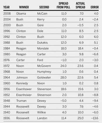
Table 1 shows the support for the two major party candidates in the final Gallup poll before presidential elections since 1936. We show the spread between the two major candidates as reported in the poll and the actual spread in the election. The last column gives the error that is the difference between the poll and the actual support. The margin of error is 3%.
Gallup Polls on Presidential Campaigns

The spread is the winner minus the loser. From http://www.gallup.com/poll/9442/election-polls-accuracy-record-presidential-elections.aspx. Accessed in July 2010.
The 1948 poll is famous for picking the wrong winner. One possible explanation is the quota method used to sample did not use the equal probability of selection method because of population shifts since the prewar Census of 1940. An alternative explanation for the wrong forecast is that many voters changed their minds a few days before the election (see Berinsky [Reference Berinsky2006] on data from that era). The methodology changed shortly after this election. Ignoring the 1948 election and looking at the 15 elections since 1948, the actual spread has been greater than 3% in six elections. An error of this size and frequency is significantly more than one would expect if the chances of such an offset was truly one out of 20.Footnote 6
If the margin of error of the spread is half of 1.96 standard errors, researchers are using a confidence interval with a smaller likelihood than 0.95, as Prob(|Z| < 1.96/2) = 0.67. That is, about one-third of the time the spread will be greater than 3% if the null hypothesis is true. This latter number is closer to what we observe. We postdict five of the Gallup polls will have a spread of greater than 3%. We observe six such polls, which is close to what we expect. It is very unlikely that the correct probability is one out of 20 and hence the 95% confidence interval does not correspond to a 3% spread.Footnote 7
EXAMPLES FROM SELECTED POLLS IN 2008
Looking at a recent election, we see that the margin of error connected with the spread gives a smaller confidence interval than 95%. Consider several polls of the 2008 presidential election. Real Clear Politics (RCP) reported the polls of 21 battleground states.Footnote 8
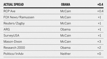
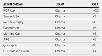
RCP reported the average of several polls for each state. In all cases in which the spread was greater than 3%, the RCP average correctly predicted the winner of the election in the state. Between three and seven polls are listed. Table 2 and table 3 take data from the two charts with seven polls. These two cases are the states with the most data displayed.
North Carolina 2008: McCain vs. Obama

Data from Real Clear Politics. Accessed November 2011.
Pennsylvania 2008: McCain vs. Obama

Data from Real Clear Politics. Accessed November 2011.
In table 2 we see one poll in North Carolina missed the actual result by more than the three points of error. Newspaper readers or online viewers are likely to say this is not bad, but the failure rate is much worse than one out of 20. In table 3 five of the seven polls report a spread greater than the margin of error. In fact, only four of the 22 states (Missouri, Montana, North Dakota, and Virginia) have all polls within the margin of error. We conclude that the margin of error of the spread in these polls is greater than what is conventionally believed.
DISCUSSION
Why has the larger error of the spread gone almost unnoticed? The examples above give hints to an answer. First, notice in all states in which the RCP average showed a spread greater than 3 percentage points the correct winner was predicted. RCP also tends to correctly identify the winner in the cases with close races. This makes sense: the candidate who is more preferred, but whose support is within the margin of error, is likely to be ahead in the race. The confidence level used to conclude that the candidate is ahead is less than 95%. Correct predictions may occur frequently enough for observers not to question the routine. If the correct winner was predicted, pundits tend not to be concerned with the size of the victory.
In the case of the Gallup polls, again beginning after 1948, the polls correctly predicted the winner whenever the spread in the final poll was at least the 3% margin of error. Correctly identifying the winner was historically a main objective. As expected, the poll also tends to correctly predict the winner in cases that are considered too close to call. The chances of winning are less than pundits believe.
Another factor is that the null hypothesis, the two candidates have equal support, often is known by analysts to be false when we move below presidential races. The majority of congressional races are not competitive. Using data immediately after the 2010 elections, 79.0% of the House of Representative contests were landslides. A landslide is defined as the winning candidate receiving greater than 55.0% of the two-party vote. Furthermore, 88.6% of the winning candidates had at least 53% of the two-party vote.Footnote 9 A poll easily identifies the winner in the majority of cases although the sampling distribution around the point estimate of the spread is wider than has been believed.
If the Gallup data are typical, polls tend to correctly predict the outcome of elections even when observations are within the margin of error. It may be difficult, using intuition alone, to distinguish between odds of one out of 20 versus many noncompetitive races with more extreme odds, say, one out of 100. Such elections are combined with other elections with odds of perhaps one out of 10 or even one out of three. These three classes of elections—lopsided, those near the margin of error, and close races—are mixed together. Although pundits have the wrong odds, most elections are lopsided and correctly predicted. Hence there is no hint that the odds are incorrect.
Also, the standard error decreases as the square root of the number of observations. The spread needed for a 95% confidence interval with about 1,000 observations is 6%, twice of what is commonly reported. Surveys with about four times more respondents will obtain the desired 3% margin of error of the spread. RCP, by averaging between three and seven polls, does generate the desired sample size for a margin of error of the spread to be 3 percentage points. Of course, take care in averaging because of the variation in methods between different polling organizations.Footnote 10
Finally, many reported polls currently exist. Readers may intuitively combine the results and sense the probability of a win in a given election. Even if the probability of error is larger than reported, it is unlikely that several polls will simultaneously report an error in the same direction due solely to sampling. For example, in the case of the 2008 New Hampshire primary some polling organizations erred by underestimating the turnout of women voters. This gave a ready explanation for those who incorrectly forecast an Obama win, thereby obscuring issues of sampling.
In conclusion, in cases with a dichotomous variable, such as a two-candidate race, the commonly reported margin of error used in reporting the spread between candidates is half of the correct value: there are not two independent estimates of support. The increase in support for one candidate results in a decrease in support for the other. Researchers need to be attentive to determining the correct confidence interval for such surveys.