1. Introduction
Analyzing problems in both the spatial and the temporal dimensions is related to the study of mechanisms that generate spatial patterns with the passage of time or more generally to the concept of morphogenesis.
Mechanisms generating patterns in spatial domains have been extensively studied in biology, where the question of ‘how the leopard got its spots’ summarizes many of the questions that biologists try to answer (e.g., Levin and Segel, Reference Levin and Segel1985; Okubo and Levin, Reference Okubo and Levin2001; Murray, Reference Murray2003). In biology the mechanism for studying morphogenesis is the classic Turing mechanism of diffusion-induced instability (Turing, Reference Turing1952) which is applied to the so-called reaction-diffusion, inhibitor–activator dynamical systems.Footnote 1 In economics, pattern formation is more often referred to as agglomeration formation and has been extensively studied in the context of new economic geography models (e.g., Krugman, Reference Krugman1996; Fujita et al., Reference Fujita, Krugman and Venables1999). Agglomerations are related to the market potential of a given location relative to others, increasing returns, transportation costs and spillover spatial effects from one site to the other that affect the evolution of economic variables such as productivity or knowledge accumulation.
In environmental and resource economics, the spatial dimension has been introduced mainly in the context of fishery management with the use of metapopulation models to study harvesting rules or reserve creation (e.g., Sanchirico and Wilen, Reference Sanchirico and Wilen1999, Reference Sanchirico and Wilen2001, Reference Sanchirico and Wilen2005; Smith and Wilen, Reference Smith and Wilen2003; Sanchirico, Reference Sanchirico2005; Wilen, Reference Wilen2007; Costello and Polasky, Reference Costello and Polasky2008). More recently Brock and Xepapadeas (Reference Brock and Xepapadeas2005, Reference Brock and Xepapadeas2008, Reference Brock and Xepapadeas2010), by using continuous spatial dynamic processes (see also Smith et al., Reference Smith, Sanchirico and Wilen2009), generalized the concept of Turing diffusion-induced instability to dynamic optimization problems and studied pattern formation and agglomeration emergence in optimal control problems with applications to resource management.
When it comes to combined environment and development issues, spatio-temporal analysis of problems means that in terms of the environmental aspect one can study the movements and the emerging spatial pattern of resource concentration, while in terms of the development aspect one can study issues such as the spatial distribution of capital stock, GDP per capita, or growth across spatial locations which could be countries or geographical regions. In this sense the interactions of pattern formation and agglomeration mechanisms could provide useful insights regarding the joint development processes and evolution of spatial concentrations of resources which are characterized by spatial movements across locations.
In this paper, I present the tools for studying these issues by using continuous spatial dynamic processes, and provide some examples regarding the ways that these tools have been used in the literature.
2. Modeling spatial movements and interactions
Let x(t, z) denote the concentration of biological or economic variables at time t ≥ 0 at the spatial point z ∈ Z, where space is assumed to be one-dimensional and modeled by a line segment.Footnote 2 The real function x(t, z) describes the state of the system.Footnote 3 The classic approach for modeling spatial movements of this state variable is through diffusion. In this context diffusion is a process through which the microscopic irregular motion of an assemblance of particles such as cells, chemicals, animals, or resources results in a macroscopic regular motion of the group. This classical approach to diffusion implies that diffusion has local or short-range effects. A measure of diffusion is the diffusion coefficient, or diffusivity, which measures how efficiently the particles move from high to low density. Let f(x(t, z), u(t, z)) be a growth function or a source for the state function that depends on the density of the state of the system, where u(t, z) is a control function, defined in the same way as the state function such as harvesting by economic agents. Let φ(t, z) denote the flow of ‘material’ such as animals or commodities past z at time t. The classic assumption is that this flux is proportional to the gradient of the concentration of material or  , where Dx is the diffusion coefficient and the minus sign indicates that material moves from high levels of concentration to low levels of concentration. Under this assumption, the evolution of the material's stock in a small interval Δz is defined as

If we divide the equation above by Δz and take limits as Δz → 0, then the spatio-temporal evolution of our state will be determined by the partial differential equation:Footnote 4

We will assume that the spatial domain is finite with z ∈ [−Z, Z]. Spatial boundary conditions for (1) could imply: (i) that the spatial domain is a circle or x(t, −Z) = x(t, Z) for all t, (ii) hostile boundaries or x(t, −Z) = x(t, Z) = 0 for all t, or (iii) zero flux at the boundaries  for all t. If the source term represents logistic population growth and the control function u(t, z) represents harvesting at spatial point z and time t or f(x, u) = x(t, z)(s − rx(t, z)) − u(t, z), then we obtain the Fisher equation:
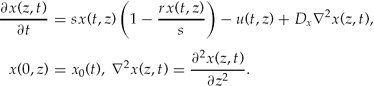
The Fisher equation can be generalized to several interacting species or activities. With two interacting species (x(t, z), y(t, z)) which are both harvested at rates (ux(t, z), uy(t, z)) and diffuse in space with constant diffusivities (Dx, Dy), respectively, we obtain


System (3–4) is referred to as a reaction-diffusion system or as an interacting population diffusion system.Footnote 5 If species x promotes the growth of y, then x is an activator, while if y reduces the growth of x, then y is an inhibitor. In this case the system (3)–(4) is an activator–inhibitor system. In systems like (3)–(4) patterns may emerge as the result of Turing diffusion-induced instability.
In many cases, however, it is necessary to model nonlocal or long-range spatial interactions. This is done by using an integral equation formulation. In the presence of nonlocal effects the temporal change of the state variable at spatial point z depends on the influence of neighboring state variables in all other locations z′. In this case the spatio-temporal evolution of the system's state, which is analogous to (1) is as follows:

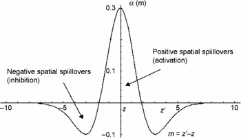
where again the spatial domain is finite with z ∈ [ − Z, Z] and spatial boundary conditions could be similar to (1). In (5), w(z − z′) is the kernel function which quantifies the effects on the state x(t, z) at z from states in others locations z′ ∈ [ − Z, Z]. A typical kernel function is presented in figure 1. It should be noted that we allow for positive and negative spatial effects.
A kernel function.

Nonlocal effects and the integral equation formulation are widely used in economics to model knowledge or productivity spillovers on the production function (e.g., Lucas, Reference Lucas2001; Lucas and Rossi-Hansberg, Reference Lucas and Rossi-Hansberg2002) or to model long-range effects of knowledge accumulation (e.g., Quah, Reference Quah2002). For example, a constant returns to scale production function with spatial knowledge spillovers can be written as

where Q is the output, L is the labor input, K is the physical capital, X is the land, and V is the productivity spillover which depends on how many workers are employed at all other locations. The spatial productivity externality is defined as exp(γV(z)), with V(z) = δ ∫−ZZe −δ|z − z′|L(z′)dz′. The function e −δ|z − z′| is the kernel. The productivity externality is a positive function of labor employed in all areas and is assumed to be linear and to decay exponentially at a rate δ with the distance between z and z′. The idea is that workers at a spatial point benefit from labor in nearby areas, and thus the distance between firms determines the production of ideas and the productivity of firms in a given region. A high δ indicates that only labor in nearby areas affects production positively.Footnote 6 In terms of agglomeration economics, the production externality is a centripetal force, i.e., a force that promotes the spatial concentration of economic activity.
Nonlocal effects are regarded as more appropriate for the analysis of problems where only economic variables are involved, whereas local effects are more appropriate for the analysis of environmental and resource management problems. In the rest of this paper, I will concentrate on local effects.
3. Turing instability and economic behavior
The idea behind spatial pattern formation through the Turing mechanism can be presented as follows. It is expected that spatial local diffusion will eventually smooth out spatial patterns and produce a homogeneous landscape, or a flat landscape. Turing suggested that on reaction-diffusion, inhibitor–activator systems, where states move in space at different speeds, local diffusion might trigger, under certain parameter values and contrary to what might have been expected, the emergence of spatial patterns. To examine conditions that would generate spatial patterns, Turing suggested that it would be sufficient to study conditions under which a system that is at a stable spatially homogeneous steady state could be destabilized by the introduction of spatial diffusion of the system's states. The idea is that if the stable flat state is destabilized when the state starts moving in space due to the diffusion perturbation, then with the passage of time the system will not return to its original spatially homogeneous state and spatial patterns will start emerging.
The mechanism can be presented using system (3)–(4), by introducing, in addition to the Turing set-up, economic behavior which is formulated by economic agents choosing the controls. The economic agents are located on the spatial domain and decide about harvesting at each site, that is they choose controls at each site z.Footnote 7 Assume that economic agents choose the controls in (3)–(4) in a certain feedback form ux = g 1(x, y, b), uy = g 2(x, y, b), where b is a vector of economic parameters (e.g., prices, unit costs). The feedback controls could be the result of behavior such as optimization, imitation, rule of thumb, open access competition. Then the system (3)–(4) can be written as
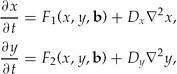

To define a spatially homogeneous steady state or flat steady state (FSS), set Dx = Dy = 0 and then define the FSS as (x*, y*): Fi(x*, y*, b) = 0, i = 1, 2. The FSS will be locally stable to temporal perturbation if the eigenvalues of the Jacobian matrix of the linearization of (7)–(8) evaluated at the FSS (x*, y*) are negative or have negative real parts. Let this Jacobian be

Therefore, the linearization of (7)–(8) at the FSS will be
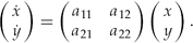
Assume that tr(J) = a 11 + a 22 < 0, det(J) = a 11a 22 − a 12a 21 > 0. This implies that the Jacobian matrix of the linearization has two real negative eigenvalues, thus the FSS is locally stable to spatially homogeneous perturbations. Introduce now spatial perturbations and consider spatial-dependent solutions of the form
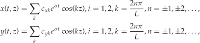
where k is called the wavenumber and 1/k, which is a measure of the wave-like pattern, is proportional to the wavelength ω: ω = 2π/k = L/n at mode n. σ is the eigenvalue, which determines temporal growth and cik, i = 1, 2 are constants determined by initial conditions and the eigenspace of σ. These trial solutions should be understood as deviations from the FSS (x*, y*).
Assume that −Z = 0, Z = L so that the spatial domain has length L and that furthermore the spatial domain is a circle. Substituting (11) into (9)–(10) and noting that they satisfy circle boundary conditions at z = 0 and z = L, we obtain the following result:
Behavior of economic agents as implied by choosing controls according to feedback rules gi(x, y, b), i = 1, 2 in the management of a reaction-diffusion system, generates spatial patterns around a flat steady state if
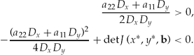
For the proof, see Brock and Xepapadeas (Reference Brock and Xepapadeas2010, theorem 1).
If the above conditions are satisfied, then when the spatially heterogeneous perturbations are introduced, one of the eigenvalues of the linearization matrix of (10) is positive, and therefore the steady state FSS (x*, y*) is locally unstable. This result means that once the states start moving within the spatial domain with different speeds, then a spatial pattern starts emerging. This pattern will not die out, but it will continue growing with the passage of time along the positive eigenvalue. Since the Jacobian matrix depends on the vector of economic parameters b, the economics of the problem contributes to the emergence or not of spatial patterns. Brock and Xepapadeas (Reference Brock and Xepapadeas2010) show that spatial patterns can be sustained in the long run in a semiarid system with states plant biomass and ground water, where economic agents harvest the plants either as profit maximizers or as open access competitors.
The local instability analysis around the steady state suggests that a spatial pattern starts emerging, but does not provide firm indications about the structure of the spatial pattern that the system will eventually settle at the steady state, since the eigenvalues analysis of the linearized system is valid only in the neighborhood of the FSS.
The steady state spatial pattern can be determined by solving the system (7)–(8) at the steady state, where  . Then the system becomes
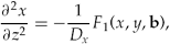
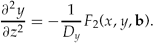
System (13)–(14) is a second-order system of ordinary differential equations in the spatial domain. Solution of this system with appropriate spatial boundary conditions will provide the steady state spatial pattern for the stocks of the system.
4. Optimal diffusion-induced spatial instability
In the analysis in the previous section, economic agents act myopically in both the temporal and the spatial dimensions, and do not take into account the spatial externality since they ignore the impact of their own harvesting on the stocks located on the sites of other agents, which emerges through the movement of stocks under the influence of diffusion. The spatial externality, as well as the temporal externality, can be taken into account by a social planner or a regulator that chooses harvesting rules by maximizing the present value of an objective over the entire spatial domain subject to the spatio-temporal evolution of the state variables. The planner's problem can be written as:

A maximum principle for this problem has been derived by Derzko et al. (Reference Derzko, Sethi and Thompson1984) (see also Brock and Xepapadeas, Reference Brock and Xepapadeas2008).Footnote 8 To use this maximum principle we need to introduce the Hamiltonian function

where p = (px, py) is the vector of the costate variables. The Hamiltonian function (16) is a generalization of the ‘flat Hamiltonian’
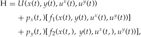
for Dx = Dy = 0. The first-order conditions for the optimal control vector u*(t, z) = (ux*(t, z), uy*(t, z)) imply uj*(t, z) = arg maxu j*H(x(t, z),y(t,z), u(t, z),p(t, z)),j = x,y. Assuming that the Hamiltonian function satisfies appropriate concavity assumptions, uj*(t, z) is defined, for interior solutions, by
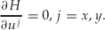
Optimal controls are then defined in terms of the state and the costate variables as

The costate variables satisfy

where g*(x(t, z), y(t, z), p(t, z)) is the vector of the optimal control functions defined by (18). Note that the costates are interpreted as the shadow prices of the stocks and that the diffusion term in (20) has a negative sign, while the diffusion term for the states of the system (system (3)–(4)), which reflect stock quantities, has a positive sign according to classic diffusion. This change in the sign of the diffusion coefficient means that prices and quantities move in the opposite directions in the spatial domain, for the optimally controlled system. This result is in agreement, as it should be, with the economic intuition.
Finally the following temporal and spatial transversality conditions should be satisfied at the optimum

The reaction diffusion system of (3) and (4) with u = (ux, uy) replaced by the optimal controls u* = g*(x(t, z), y(t, z), p(t, z)) and the system of (20) constitute a system of four partial differential equations. This is the modified Hamiltonian dynamic system, or simply Hamiltonian system, which along with the initial conditions and the transversality conditions (21) determine the spatio-temporal evolution of the state and costate variables along the socially optimal path.
In order to analyze pattern formation at the social optimum we examine the stability of a flat optimal steady state (FOSS) of the Hamiltonian system to spatially heterogeneous perturbations. The Hamiltonian system can be written in a compact way, where subscripts t, z denote partial derivatives with respect to t and z, respectively, in order to simplify notation, as
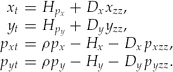
A FOSS is defined, from the Hamiltonian system (22), as a quadruple (x*, y*, p*x, p*y):xt = yt = pxt = pyt = 0 for Dx1 = Dx2 = 0. It is known from the work of Kurz (Reference Kurz1968) that such a FOSS will either be unstable or will have the saddle point property. Assume that the FOSS (x*, y*) has the local saddle point property which means that the Jacobian matrix of the linearization of (22) has two positive and two negative eigenvalues. To study pattern formation due to spatial diffusion around the FOSS, we linearize (22) at the FOSS and we introduce again solutions in the form of the following spatial perturbations:

These trial solutions should be understood as deviation from the FOSS (x*, y*). Brock and Xepapadeas (Reference Brock and Xepapadeas2010) derive conditions under which the Jacobian matrix of the linearized spatially perturbed system has three or four real positive eigenvalues or complex eigenvalues with positive real parts. Brock and Xepapadeas (Reference Brock and Xepapadeas2008) derive similar conditions for a system with one state variable. In this case the spatially perturbed FOSS is unstable with two real positive eigenvalues or complex eigenvalues with positive real parts.
This result implies that a spatial pattern is emerging for the optimally controlled price quantity system, where prices are represented by the costate variables and quantities by the state variables. The pattern does not die out with the passage of time since it grows in time along the positive eigenvalues.
This is the optimal diffusion-induced instability since it emerges in the context of a dynamic optimization problem, where the classic Turing diffusion-induced instability is not the result of dynamic optimization.
The intuition behind this result can be described as follows. Controlling the system to a FOSS along the stable manifold is costly for the social planner. When spatial perturbations are introduced, the benefit-cost ratio of controlling the system to the FOSS depends on the spatial mode n. If there is a mode such that the benefit-cost ratio is less than one, then it is optimal not to control the system to the FOSS but to let it go unstable at this mode, which is the unstable mode. It turns out that the unstable mode is the one for which the negative eigenvalue turns to positive. Thus a socially optimal spatial pattern starts emerging at the unstable mode. In the terminology of new economic geography, the regulator generates an optimal agglomeration.
Brock and Xepapadeas (Reference Brock and Xepapadeas2008, Reference Brock and Xepapadeas2010) have identified conditions for the emergence of optimal diffusion-induced instability, or the emergence of optimal agglomeration for two problems. The first is the social management of a shallow lakeFootnote 9 with spatial diffusion of the accumulated phosphorous stock on the lake, and the second is the social management of a semiarid system with plant biomass and ground water diffusion.
The local optimal instability analysis around the FOSS suggests that an optimal spatial pattern starts emerging, but again does not provide firm indications about the structure of the spatial pattern regarding the state and the costate (shadow prices) in the long run. The optimal long-run spatial pattern, if it exists, can be determined by solving the system (22) for xt = yt = pxt = pyt = 0. Then the system becomes
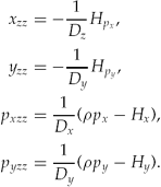
System (23) is a second-order system of ordinary differential equations for the states and costates, or the quantity-price system, in the spatial domain. Solution of this system with appropriate spatial boundary conditions will provide the optimal steady state spatial pattern for the stocks and there shadow prices. This analysis suggests that spatial patterns, if they emerge and persist in the long run, are most likely to be different between the case where economic agents act myopically and ignore the spatial externalities and the case where a social planner manages the system optimally by taking into account the spatial externality. This observation suggests that the type of analysis presented here could be used as a basis for regulation with spatial characteristics. In this case the social planner would explicitly design spatially dependent policy instruments such as taxes or controls with the purpose of inducing the economic agents to take decisions which would generate spatial patterns that approximate the socially optimal spatial patterns.
5. Concluding remarks
Methods for analyzing resource management in both the spatial and the temporal dimensions could be useful in understanding the mechanisms which create spatial patterns and the design of spatial regulation. The approach presented above differs – by using continuous spatial dynamics – from the main body of the existing literature, which uses metapopulations and discrete spatial-dynamic models (e.g., Smith et al., Reference Smith, Sanchirico and Wilen2009). This increases the mathematical complication since it introduces distributed parameter systems and optimal control of partial differential equations in modeling. On the other hand, however, it significantly reduces the dimensionality of the optimal control problems resulting from metapopulation models, which require one state variable for each patch. This might make it easier to study models with multiple state variables with interactions among themselves.
The analysis and the examples presented here were restricted to resource management. However, pure economic variables, such as capital, knowledge, or productivity effects, have a spatial dimension and move across location, which, due to the nonlocal characteristics of the spatial effects, can be better modeled by integral kernels. Combining local and nonlocal effects might produce interesting results regarding the emergence of spatial patterns and agglomerations on combined ecological and economic models. Furthermore persistent nonhomogeneous spatial patterns on economic variables, such as per capita capital or per capita gross domestic products across countries, would suggest that the growth process does not produce economic homogeneity across geographical regions. This is an important issue in economic development and the methods presented here could be useful for analyzing it.