1. Introduction
As robotic technologies continue to be upgraded and modernized, they are gradually replacing humans in various fields to perform complex, tedious, and risky tasks. This substitution not only improves work efficiency but also reduces the cost to humans in accomplishing these tasks. Many factories have successfully utilized robots to completely replace humans in their work, realizing concepts such as unmanned factories and smart factories [Reference Simic, Dabic-Miletic, Tirkolaee, Stevic, Ala and Amirteimoori1–Reference Ramos, Pinto and Haddad5]. However, as the size of factories increases, the task locations of robots are no longer limited to fixed locations. Instead, there are situations where there are multiple task points and even multiple robots performing multiple tasks simultaneously. In this multi-task point scenario, the robot no longer performs repetitive work singularly, but performs each task rationally according to the nature of the task and the actual situation [Reference Guo, Miao, Ji and Pan6,Reference Martin, Muros, Maestre and Camacho7]. Therefore, it is necessary to find the optimal task allocation scheme for the robots to maximize the benefits under various constraints, depending on the nature of the robots, their usage, and the task loads.
In essence, many robot task allocation problems are variants of the traveling salesman problem (TSP). The robot task allocation problem is a slack problem of the TSP, mainly because the robots are allocated in a way that forms a closed loop and does not include subloops [Reference Winston8,Reference Lee, Lee, Masoud, Krishnan and Li9]. Therefore, many scholars apply some simple variations of algorithms and methods for solving the TSP and the multiple traveling salesman problem (MTSP) to solve the robot task allocation problems according to the actual situation, to maximize the benefit in the robot’s execution of the task. In the robot task allocation problem for a single robot, many researchers consider the task allocation issue as a constrained TSP, thereby using heuristic intelligent algorithms for solving it [Reference Macharet and Campos10–Reference Dhanaraj, Nemlekar, Nikolaidis and Gupta12]. Xuewu et al. proposed a particle swarm optimization (PSO) algorithm enhanced with L
 $\acute {e}$
vy flights to address the path planning issues of spot welding robots. They treated the path planning problem for welding robots as a TSP and solved it using a L
 $\acute {e}$
vy flight-based PSO [Reference Wang, Yan and Gu13]. Wu et al. perceived the trajectory of laser engraving robots as a large-scale TSP and proposed an improved two-layer ant colony optimization (ACO) to solve the model. Experiments show that this method can reduce engraving time [Reference Wu, Wu, Zhao, Feng and Liu14]. Kong et al. introduced a comprehensive heuristic fast-marching planning system that integrates task allocation, initial planning, and dynamic replanning for a robotic floating-garbage cleaning mission, in which the cleaning tasks were formulated as a TSP. The system employed a distance metric derived from the FM* algorithm to determine the optimal traversal sequence [Reference Kong, Wu, Qiu, Tian and Yu15]. Solutions to multi-robot task allocation problems can be primarily categorized into distributed and centralized approaches. In the distributed task allocation method, each robot only has information about other robots in its vicinity and calculates the tasks it needs to complete based on this information. While this method enables good scalability and allows the system to continue functioning even if one or more robots fail, it significantly risks overlooking some tasks, making the robot unable to complete all tasks [Reference Li, Tong, Li, Cong, Tong, Yamashita and Asama16–Reference Otte, Kuhlman and Sofge18]. Essentially, this approach views the task allocation for multiple robots as a MTSP to be handled and solved. Zhao et al. recognized the multi-robots multi-task allocation issue in warehouse environments as an MTSP and proposed an optimized algorithm combining a hierarchical genetic algorithm with the ACO. This method has been shown in the ROS environment to effectively reduce overall transportation time [Reference Zhao, Xu, Lu, Shi and Li19]. Li et al. treated the multi-robots task allocation problem as an MTSP and introduced a distributed cooperative task allocation strategy based on an improved gray Wolf optimization (IGWO) algorithm, which demonstrated good convergence speed and accuracy [Reference Li and Yang20]. Ma et al. proposed an end-to-end task allocation framework to autonomously and intelligently distribute multiple tasks among a robot fleet, addressing this variant of the MTSP through a combinatorial optimization approach [Reference Ma, Ruan, Du, Bucknall and Liu21].
The MPA, proposed by Faramarzi et al. in 2020, is a nature-inspired metaheuristic based on the foraging behavior of marine predators [Reference Faramarzi, Heidarinejad, Mirjalili and Gandomi22]. It exhibits fast convergence speed, high solution accuracy, and simple parameter settings, demonstrating strong global search capability in continuous optimization problems [Reference Elaziz, Mohammadi, Oliva and Salimifard23–Reference Wang and Huang25]. However, when applied to complex or high-dimensional tasks-especially discrete or combinatorial optimization problems-the original MPA suffers from limited population diversity and a tendency to get trapped in local optima, which weakens its global exploration performance. Consequently, numerous studies have sought to improve its exploration–exploitation balance. For example, Ma et al. [Reference Ma, Chang, Lin, Zhang, Song and Chen26] introduced a teaching–learning mechanism to enhance population diversity and alleviate premature convergence. Ramezani et al. [Reference Ramezani, Bahmanyar and Razmjooy27] proposed an improved MPA integrating opposition-based learning, a chaos map, and self-adaptive population dynamics, which effectively diversifies the initial population and accelerates escaping from local optima. Oszust [Reference Oszust28] further designed an enhanced MPA incorporating a local escape operator (LEO) to strengthen global exploration. Experiments confirmed that the LEO-MPA achieves superior performance compared with the conventional MPA.
Based on the above analysis, although various traditional meta-heuristic algorithms have been widely applied to robot task allocation problems, they often suffer from issues such as premature convergence, insufficient population diversity, and performance degradation in large-scale or constrained optimization scenarios. These issues are particularly pronounced in combinatorial optimization problems, such as the TSP, single-robot task allocation with strict time windows, and multi-robot task allocation, where the search space is discrete, highly complex, and prone to getting stuck in local optima. The marine predator algorithm (MPA), inspired by the foraging behavior of marine predators, has demonstrated robust global search capabilities, rapid convergence, and simple parameterization in continuous optimization problems. However, due to the mismatch between the continuous search mechanism and the representation of discrete solutions, the direct application of this algorithm to discrete sequence optimization remains challenging. To overcome these limitations, this paper proposes a new marine predator NMPA based on the MPA framework. By redesigning the encoding mechanism and introducing pheromone-guided Brownian motion alongside an adaptive search strategy, the proposed NMPA effectively enhances population diversity, strengthens global exploration capabilities, and achieves a better balance between exploration and exploitation. Consequently, the algorithm effectively avoids local optima and improves convergence efficiency. Furthermore, the proposed NMPA algorithm has been applied to three representative models, including the TSP, a single-robot task allocation model with strict time windows, and a multi-robot task allocation model. Comparative experiments demonstrate that the NMPA algorithm outperforms traditional meta-heuristic algorithms in terms of solution quality, convergence performance, robustness, and time efficiency. Based on this, the main contributions of this paper are summarized as follows:
-
1. Algorithmic redesign for discrete optimization: Since the traditional MPA is not suitable for discrete sequence problems, we redesign the motion search pattern and encoding mechanism to enable efficient handling of discrete robot task allocation models.
-
2. Pheromone Brownian motion strategy: We introduce a pheromone-driven Brownian motion mechanism that enhances the exploration capability of the algorithm, allowing it to effectively identify promising search directions during the early search phase and avoid premature convergence.
-
3. Comprehensive application and validation: The proposed NMPA is applied to multiple robot task allocation models, demonstrating excellent solution quality, convergence stability, and cross-model generality.
2. Marine predator algorithm
The MPA primarily models the behavior of a predator that selects the most effective foraging strategy either L
 $\acute {e}$
vy or Brownian wandering, to feed on its prey. Thus, the core search strategies of the MPA consist of these two wandering techniques. In this algorithm, the predator symbolizes the current optimal solution, while the prey denotes the solution post the current search iteration. The MPA is structured into four main components.
-
1. Formation of the sea: This primarily involves the formation of the predator and prey.
-
2. Predation: In this phase, the predator searches for and preys upon the prey. The predation process is subdivided into three stages: the exploration stage, the transition stage between exploration and exploitation, and the exploitation stage.
-
3. Vortex formation and FADs effect: During the exploration phase, predators may need to swim longer distances in various areas to locate a new environment where prey is distributed. Within the algorithm, fish aggregating devices (FADs) are viewed as optimal solutions. Proposals are made to prevent stagnation due to entrapment in local optima.
-
4. Updating of the sea: This phase assesses the current positions of the predator and prey to facilitate the identity transformation between the predator and prey.
3. Strategy improvement of marine predator algorithm
Although several improved variants of the MPA have been extended to handle discrete optimization problems through customized encoding or discretization schemes, the original MPA was primarily designed for continuous domains and thus faces challenges in effectively optimizing discrete sequence-based problems such as the robot task assignment problem and the TSP. Therefore, this paper proposes a redesigned MPA framework to better adapt to discrete search spaces and improve its performance in combinatorial optimization.
3.1. Discretization and improvement of Brownian motion
3.1.1. Discretization of Brownian motion
Brownian motion (
 $Bm$
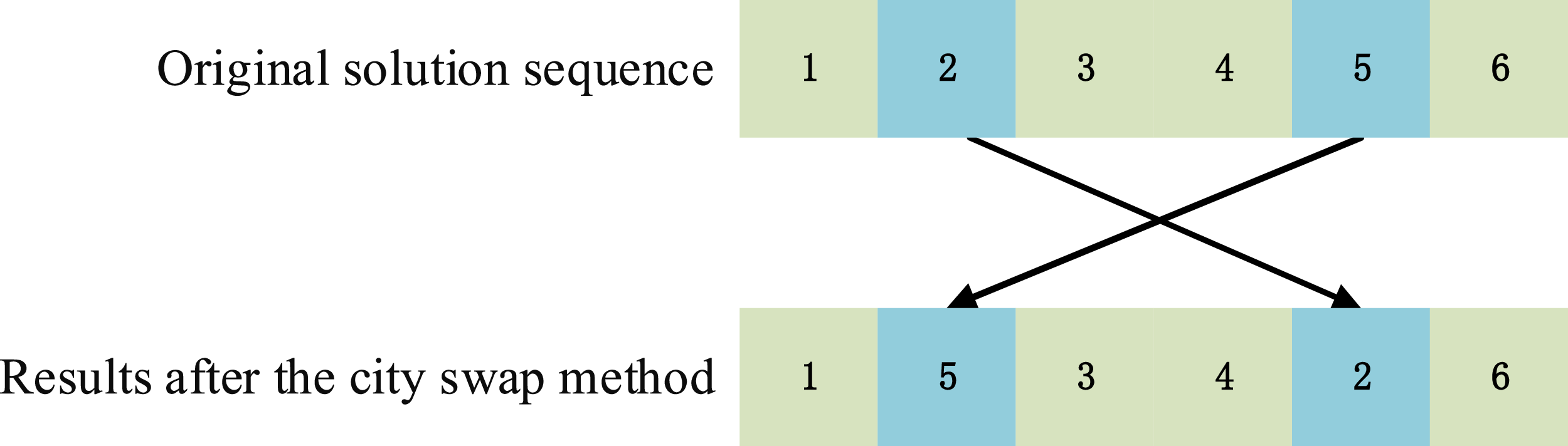
) is the ceaseless, irregular movement of particles suspended in a fluid or gas. In the traditional MPA, Brownian motion is represented by a normally distributed random vector. However, since the optimization target in the TSP is not a continuous variable but a discrete sequence of travels, a different approach is necessary. In this context, the city exchange method is utilized to simulate the Brownian wandering of the predator in the ocean. This method involves randomly swapping the positions of two cities in the sequence, as illustrated in Figure 1, it is the process of perturbing sequences using urban exchange method. In addition, we have demonstrated in the Appendix A that the city exchange method is a random walk method that conforms to Brownian motion for discrete sequences.
City swap method.

Pheromone-based Brownian motion.

3.1.2. A Brownian motion with pheromones(
 $Bmp$
)

In the early stages of the marine predator algorithm, prey predominantly utilize Brownian motion to explore the ocean, aiding in expanding the search range. However, as the process progresses, aimless exploration can negatively impact both the speed and direction of convergence. To address this issue, a modified Brownian motion incorporating pheromones is introduced to guide the prey toward optimal exploration directions. The concept of pheromones was originally developed by Dorigo et al. in the ACO, where it was used to form new solutions during ant colony explorations [Reference Colorni, Dorigo and Maniezzo29].
This study adapts the pheromone concept to facilitate more structured exploration. Multiple cities whose order needs to be exchanged are randomly selected, and a pheromone-enhanced roulette method is employed to integrate these cities into the solution sequence, as illustrated in Figure 2. This approach not only maintains the stochastic nature of the wandering method but also directs the search toward promising areas. The pheromone update formulas used in this method are detailed in Eqs. (1–4).
The probability that the cities that need to perform the exchange order are selected:
 \begin{align} P_{ij}^{k}=\left \{ \begin{matrix} \dfrac {{{[ {{\theta }_{ij}} ]}^{\alpha }}{{[ {{\eta }_{ij}} ]}^{\beta }}}{\underset {r\notin \text{ }\!\!\text{ }tab{{u}_{k}}}{\mathop {\sum }}\,{{[ {{\theta }_{ir}}]}^{\alpha }}{{ [ {{\eta }_{ir}} ]}^{\beta }}}\,\,\,\,\,j\notin \text{ }\!\!\text{}tab{{u}_{k}} \\ \,\,\,\,\,\,\,\text{ }\!\!\,\!\!\text{ 0}\,\,\,\,\,\,\,\,\,\,\,\,\,\,\,\,\,otherwise\text{ }\!\!\,\!\!\text{ } \\ \end{matrix} \right . \end{align}
where
 ${\eta }_{ij}$
is the heuristic factor between the current city
 $i$
and the next city
 $j$
;
 ${\theta }_{ij}$
is the concentration of pheromone left by the prey between the current city
 $i$
and the next city
 $j$
; and
 $tab { u } _ { k } \, [ k = 1,2,3\ldots ]$
is known as the taboo list and is used to keep track of the cities that ant
 $k$
has visited. The
 $ \alpha$
is the pheromone factor, implying the importance of the path with respect to the remaining pheromone, and the
 $ \beta$
is the heuristic factor, indicating the influence of the heuristic information.
Pheromone volatilization formula:
 \begin{align} {{\tau }_{ij}}=\left ( 1-\rho \right ){{\tau }_{ij}}\left ( t \right ) \end{align}
where
 $ \rho$
is the rate of volatilization.
The
 $k$
th prey releases a pheromone formula for the path it passes through:
 \begin{align} \Delta t_{ij}^k\left ( t \right ) = \left \{ \begin{array}{l} \dfrac {Q}{{{d_{(ij)}}}}\,\,\left ( {i,j} \right )\in {T^k}\\ 0\,\,\,\,\,\textrm {{ otherwise}} \end{array} \right . \end{align}
where
 $Q$
is a constant;
 ${T}^{k}$
is the path of the prey
 $k$
; and
 ${d}_{(ij)}$
is the length of the current path, when
 ${d}_{(ij)}$
is smaller, more pheromone will be obtained on the current path.
Pheromone update formula:
 \begin{align} {{\tau }_{ij}}\left ( t+1 \right )=\left ( 1-\rho \right ){{\tau }_{ij}}\left ( t \right )+\sum \limits _{k=1}^{m}{\Delta t_{ij}^{k}\left ( t \right )} \end{align}
2-opt method.

3-opt method.

3.2. Replacement of L
$\acute {e}$
vy flightwalker

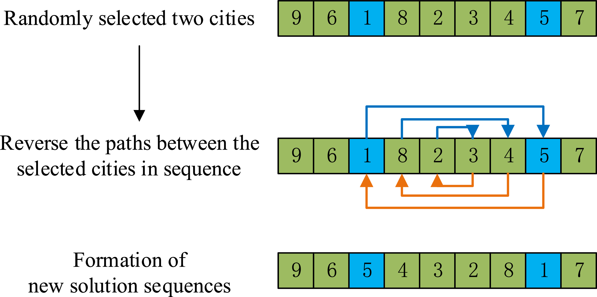
The 2-opt and 3-opt are classical optimization operators used in the problems of sequence of traversal. The 2-opt improves the path by reversing a segment between two arbitrarily chosen cities. Specifically, the algorithm selects two cities, reverses the path between them, and forms a new path. If the total length of this new path is shorter than the original, it replaces the current path, as illustrated in Figure 3. On the other hand, the 3-opt starts by randomly selecting two cities to divide the solution sequence into three segments. It then explores various possible reconnections of these segments to create eight new paths. Among these, the path with the shortest length is chosen as the current path, as shown in Figure 4.
The 3-opt is generally more efficient than the 2-opt as it can more effectively avoid local optima through its broader search strategy. However, it is also more computationally demanding because it evaluates eight different paths, which can pose significant challenges in large-scale applications.
In the context of the MPA, the L
 $\acute {e}$
vy wandering strategy is applied during the middle and late stages of the algorithm to rapidly converge to the optimal value and avoid local optima. This paper utilizes a combination of 2-opt and 3-opt within different phases of the algorithm’s exploration. During the middle stage, 2-opt is primarily used to facilitate quick escapes from local optima and explore new, high-quality areas at minimal cost. In the late stage, 3-opt is employed to ensure a thorough escape from any remaining local optima, ultimately guiding the search towards the global optimum. This strategic use of both operators enhances the convergence of the algorithm’s efficiency in complex solution spaces and results of the global optimal solution.
3.3. Information exchange between predator and prey
In the MPA, predators symbolize individuals within the search process, striving to locate the optimal solution, akin to predators hunting for food. Preys represent candidate solutions, which may contain potentially optimal solutions. Predators attempt to pursue these preys to enhance their own positions, while the prey must similarly adjust their positions in response to the predator’s movements to evade capture.
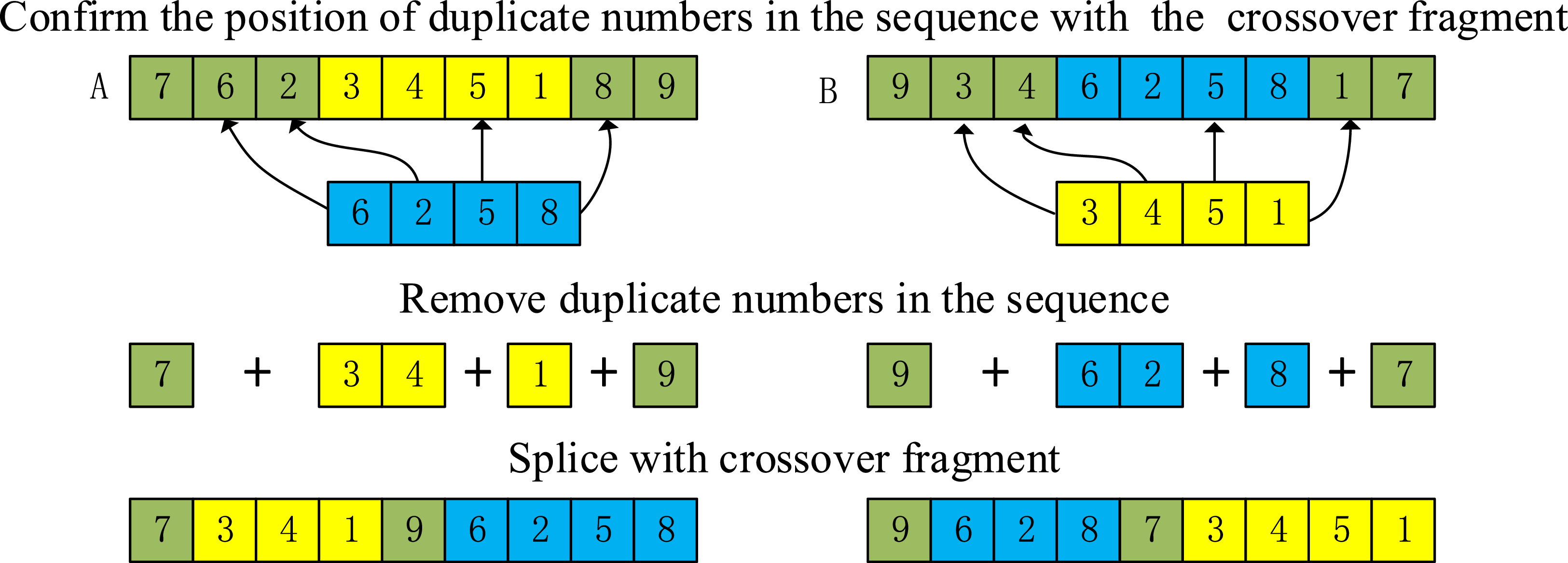
This dynamic of chase and evasion mirrors the iterative process of optimization where both predator and prey continuously refine their strategies. This paper leverages the cross-optimization operator to model the informational interactions between the predator and prey. This operator facilitates the exchange of segments between the solution sequences of the predator and the prey, enhancing the algorithm’s ability to explore and exploit the search space effectively, as depicted in Figure 5.
Information exchange between predator and prey.

Figure 5 Long description
A diagram illustrating the process of confirming, removing, and splicing duplicate numbers in sequences with crossover fragments. Panel A: The sequence A contains the numbers 7, 6, 2, 3, 4, 5, 1, 8, 9. The crossover fragment is 6, 2, 5, 8. Arrows indicate the positions of duplicate numbers in the sequence with the crossover fragment. Panel B: The sequence B contains the numbers 9, 3, 4, 6, 2, 5, 8, 1, 7. The crossover fragment is 3, 4, 5, 1. Arrows indicate the positions of duplicate numbers in the sequence with the crossover fragment. Panel C: The duplicate numbers in the sequences are removed, resulting in the sequences 7, 3, 4, 1, 9 for sequence A and 9, 6, 2, 8, 7 for sequence B. Panel D: The sequences are spliced with the crossover fragments, resulting in the sequences 7, 3, 4, 1, 9, 6, 2, 5, 8 for sequence A and 9, 6, 2, 8, 7, 3, 4, 5, 1 for sequence B.
4. The process of the novel marine predator algorithm
4.1. Formation of the sea
In the MPA, both the predator and prey are candidate solutions, making each prey within the ecosystem a potential predator. Similar to most meta-heuristic algorithms, MPA generates initial populations randomly within the search space. Specifically for the TSP, which involves finding an optimal sequence of visits to various cities, this paper employs a greedy algorithm to randomly generate
 $m$
groups of solution sequences. These sequences constitute the prey within the simulated marine environment. From these
 $m$
groups, the best-performing solution sequence evaluated based on its efficiency and cost-effectiveness is chosen as the predator.
4.1.1. Prey and predator matrix
For the discrete sequences of TSP, the traditional prey matrix (
 $P$
) and predator matrix (
 $E$
) are not able to express the discrete sequences of the TSP concretely, as shown in Eqs. (5–6). Mainly because the objective solution is related to the sequence numbers of all cities, the prey matrix and predator matrix need to be redefined as in Eqs. (7–8)
 \begin{align} pr&={{\left [ \begin{matrix} {{X}_{1,1}} & \cdots & {{X}_{1,d}} \\ \vdots & \ddots & \vdots \\ {{X}_{t,1}} & \cdots & {{X}_{t,d}} \\ \end{matrix} \right ]}_{t\times d}} \end{align}
 \begin{align} El&={{\left [ \begin{matrix} {{{{X}^\prime}}_{1,1}} & \cdots & {{{{X}^\prime}}_{1,d}} \\ \vdots & \ddots & \vdots \\ {{{{X}^\prime}}_{t,1}} & \cdots & {{{{X}^\prime}}_{t,d}} \\ \end{matrix} \right ]}_{t\times d}} \end{align}
 \begin{align} \overline {Pr}&={\left [ \begin{matrix} {{i}_{1}} & {{k}_{1}} & \ldots & {{j}_{1}} \\ {{j}_{2}} & {{i}_{2}} & \ldots & {{k}_{2}} \\ \vdots & \vdots & \ddots & \vdots \\ {{i}_{m}} & {{j}_{m}} & \ldots & {{k}_{m}} \\ \end{matrix} \right ]_{m\times n}}\text{ }i,j,k\ldots \in {{S}_{n}} \end{align}
 \begin{align} \overline {El}&={\left [ \begin{matrix} {{i}_{1}} & {{k}_{1}} & \ldots & {{j}_{1}} \\ {{j}_{2}} & {{i}_{2}} & \ldots & {{k}_{2}} \\ \vdots & \vdots & \ddots & \vdots \\ {{i}_{m}} & {{j}_{m}} & \ldots & {{k}_{m}} \\ \end{matrix} \right ]_{m\times n}}\text{ }i,j,k\ldots \in {{S}_{n}} \end{align}
where
 $Pr$
and
 $El$
are the matrices of preys and predators before improvement,
 $t$
is the population size before improvement,
 $d$
is the dimension of the search space before improvement,
 $X_{e,k}$
is the position of the current
 $e$
th prey in the
 $j$
dimension,
 ${{X}^\prime}_{1,1}$
is the vector of predators,
 $\overline {Pr}$
and
 $\overline {El}$
are the matrices of
 $m\times n$
that are the improved prey and predator,
 $m$
is the population size,
 $n$
is the total number of cities,
 $i,j,k\ldots$
is random numbers less than
 $m$
, and
 ${S}_{n}$
is the set of
 $n$
city numbers.
4.2. Optimization process of predation
4.2.1. Exploration phase
This phase occurs at the beginning of the MPA’s search of the solution space. In this phase, the prey mainly performs Brownian motion to search the ocean domain. While traditional Brownian motion is effective for quickly expanding the search range, it can lead to directionless exploration, which might eventually impede the speed and accuracy of convergence toward the optimal solution. To address these challenges, this paper introduces a collaborative search strategy involving
 $Bmp$
and
 $Bm$
. By integrating these two strategies, the algorithm ensures that while the prey is able to expand the search range swiftly, the predator is also maintained on an effective search direction. This approach helps balance broad exploration with targeted navigation, enhancing the overall efficiency and effectiveness of the search process.
Mathematical modeling of prey position updates for traditional MPA:
 \begin{equation} \begin{aligned} &\text{ While } t \leq \frac {1}{3} t_{\mathrm{max}}, i=1,2, \ldots , n \\ & \text{ stepsize }_i=R_B \otimes \left ( El_i-R_B \otimes Pr_i\right ) \\ & Pr_i= Pr_i+P \times R \otimes \text{ stepsize }_i \\ \end{aligned} \end{equation}
where
 $i$
is the number of predator or prey,
 $n$
is the maximum number of predator or prey,
 $t$
is the current iteration number,
 $t_{max}$
is the maximum iteration number.
 $R_B$
is a vector of normally distributed random numbers, which is used to represent Brownian motion.
 $\otimes$
is term-by-term multiplication,
 $R$
is a random number between
 $[0,1]$
, and
 $P$
is a constant equal to 0.5.
Mathematical modeling of prey location updates for NMPA:
 \begin{align} \begin{aligned} &\text{ While } t \leq \frac {1}{3} t_{\mathrm{max}}, i=1,2, \ldots , n \\ &\overline {{Pr}_{i}}=p*\{\overline {{Pr}_{i}}\oplus [(\overline {{El}_{i}} \oplus Bm\,\,\overline {\otimes }\,\,\overline {{El}_{i}})\\ &\,\,\,\,\,\,\,\,\,\,\odot (\overline {{Pr}_{i}}\oplus Bmp\,\,\overline {\otimes }\,\,\overline {{Pr}_{i}})]\} \end{aligned} \\[-10pt] \nonumber \end{align}
where
 $\overline {P{{r}_{i}}}$
is the current prey position,
 $p$
is the number of prey and predator movement steps in this round,
 $\overline {P{{r}_{i}}}$
and
 $\overline {{El}_{i}}$
are the sequence of the
 $i$
th prey and predator history optimal,
 $\overline {\otimes }$
is to carry out the strategy,
 $\odot$
is the MPA for information transfer,
 $Bm$
is to carry out the Brownian motion, and
 ${Bmp}$
is to carry out the Brownian motion with pheromones,
 $\oplus$
is the judgment of whether or not to accept the new position, as in Eq. (11).
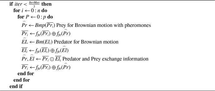
The equation represents that the predator performs Brownian motion, the prey performs Brownian motion with pheromones, and the prey moves to the optimal position after the exchange of information between the prey and the predator. In the early stages of the algorithm, the current position of the predator must not be the optimal position, and most likely is a local optimal solution. Therefore, the predator performs Brownian motion, which can escape from the local optimal solution as much as possible, and at the same time extends the search range. On the other hand, preys adopt Brownian motion with pheromones, which is mainly responsible for exploring the sea area. As the amount of data increases, the size of the sea area to be explored may also increase. Therefore, aimless exploration by preys may lead to slow convergence speed. At the same time, Prey in this phase using the strategy of Brownian motion with pheromones can enhance the directionality and effectiveness of preys search. The use of two different foraging strategies by prey and predators offer two advantages:
-
(1) It will not lead to the prey getting lost during the search process.
-
(2) The amount of information in the early stage is small, and the prey is needed to increase the amount of information to lay the foundation for the later search.
As shown in Algorithm 1, it is the simplified pseudocode for this phase.
 \begin{align} X \oplus Y = \begin{cases} X, & \text{if } f_{\text{fit}}\!\left (X\right ) \,\ge\, f_{\text{fit}}\!\left (Y\right ), \\[4pt] Y, & \text{otherwise.} \end{cases} \\[-8pt] \nonumber \end{align}
where
 ${f}_{fit}\left ( \right )$
is the objective function,
 $X$
is the left side of
 $\oplus$
,
 $Y$
is the right side of
 $\oplus$
, which means that comparing the fitness of the two sides of the historically optimal position and the new position, and selecting the side with higher fitness.
Exploration phase

Algorithm 1 Long description
An equation defining a conditional operation. The equation states that X or Y is selected based on the value of the objective function f_fit. If the value of f_fit for X is greater than or equal to the value of f_fit for Y, then X is selected. Otherwise, Y is selected. The equation uses the symbol ⊕ to represent this conditional selection operation. The variables X and Y represent the left and right sides of the ⊕ symbol, respectively. The function f_fit is used to evaluate the fitness of the two sides.
4.2.2. Exploration and exploitation conversion phase
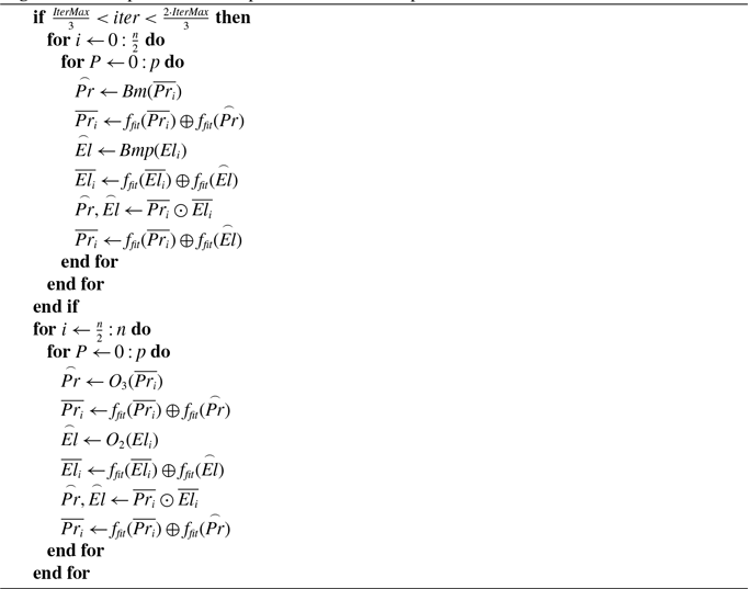
This phase occurs in the middle of the search solution space of the MPA. In this phase, half of the prey is mainly responsible for searching, and the other half is responsible for mining. This phase mainly prepares for the convergence, half of the preys eliminate the cross-over edges present in the TSP sequence by 2-opt and 3-opt, so that the half of preys quickly converge to the optimal solution, and at the same time increase the information of the sea area, which motivates the other half of the preys to carry out an effective exploration of the sea area and reduces the unnecessary searches.
Mathematical modeling of prey position updates for traditional MPA:
 \begin{equation} \small \begin{aligned} & \text{ While } \frac {1}{3} t_{\max }\lt t\lt \frac {2}{3} t_{\max }, i=1,2, \ldots , \frac {n}{2} \\ & \text{ stepsize }_i=R_B \otimes \left (R_B \otimes El_i-\text{ Pr }_i\right ) \\ & C F=\left (1-\frac {t}{t_{\max }}\right )^{\left (\frac {2 t}{t_{\max }}\right )} \\ & Pr_i=El_i+P \times C F \otimes \text{stepsize}_i \\ & \text{ While }\frac {1}{3} t_{\max }\lt t\lt \frac {2}{3} t_{\max }, i=\frac {n+1}{2},\frac {n+2}{2}, \ldots , n \\ & \text{ stepsize}_i=R_L \otimes \left (\right . \! El_i-R_L \otimes Pr \left ._i\right )\\ &Pr_i= Pr_i+P \times R \otimes \text{stepsize}_i\\ \end{aligned} \small \end{equation}
where
 $C F$
is the adaptive parameter of step size
 $\text{ stepsize}$
,
 $R_L$
is is to carry out the l
 $\acute {e}$
vy flightwalker.
Mathematical modeling of prey position updates for NMPA:
 \begin{equation} \small \begin{aligned} & \text{ While } \frac {1}{3} t_{\max }\lt t\lt \frac {2}{3} t_{\max }, i=1,2, \ldots , \frac {n}{2} \\ &\overline {{Pr}_{i}}=p*\{\overline {{El}_{i}}\oplus [(\overline {{El}_{i}} \oplus Bmp\,\,\overline {\otimes }\,\,\overline {{El}_{i}})\\ &\,\,\,\,\,\,\,\,\,\,\odot (\overline {{Pr}_{i}}\oplus Bm\,\,\overline {\otimes }\,\,\overline {{Pr}_{i}})]\}\\ & \text{ While }\frac {1}{3} t_{\max }\lt t\lt \frac {2}{3} t_{\max }, i=\frac {n+1}{2},\frac {n+2}{2}, \ldots , n\\ &\overline {{Pr}_{i}}=p*\{\overline {{Pr}_{i}}\oplus [(\overline {{El}_{i}} \oplus O_2\,\,\overline {\otimes }\,\,\overline {{El}_{i}})\\ &\,\,\,\,\,\,\,\,\,\,\odot (\overline {{Pr}_{i}}\oplus O_3\,\,\overline {\otimes }\,\,\overline {{Pr}_{i}})]\}\\ \end{aligned} \small \end{equation}
where
 $O_2$
is is to carry out 2-opt,
 $O_3$
is is to carry out 3-opt. Half of the prey performs Brownian motion with pheromones, and this part of the preys performs efficiently carries out solution space exploration, minimizing inefficient exploration. The other half of the predators performs Brownian motion to expand the exploration of the current high-quality region to avoid falling into the local optimal solution. Eventually, the prey and the predator perform information transfer and then move the position of the prey to the optimal position found by the predators and then perform a new exploration. While the other half of the preys performs 2-opt wandering to explore the optimal solution in the current high-quality space, the other half of the predators performs 3-opt wandering to enter the convergence in advance, so as to enable the other preys and predators to perform the high-quality exploration, and to avoid ineffective expansion of the search range of the prey and predator, which leads to a slow convergence speed. As shown in Algorithm 2, it is the simplified pseudocode for this phase.
Exploration and exploitation conversion phase

Algorithm 2 Long description
An equation describing prey position updates in a mathematical model. The equation is divided into two main parts, each representing different conditions and operations. The first part involves a while loop where the variable t is between one-third and two-thirds of t_max, and i ranges from 1 to half of n. The equation updates the variable Pr_i using a combination of operations involving p, El_i, and Bm. The second part involves another while loop with the same condition on t, but i ranges from (n+1)/2 to n. This part updates Pr_i using operations involving p, El_i, O_2, and O_3. The operations include various combinations of addition, subtraction, and multiplication, as well as specific functions like Bm and O_2. The equation aims to model the behavior of prey in an optimization algorithm, with different strategies for exploration and exploitation.
4.2.3. Exploitation phase
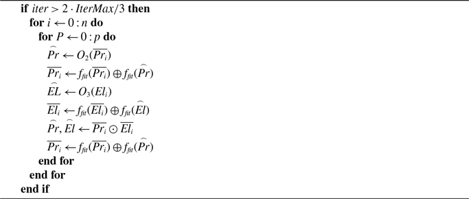
This phase occurs late in the search of the solution space by the MPA. This phase is primarily a convergence phase, so the predator performs 3-opt, and the prey performs 2-opt.
Mathematical modeling of prey position updates for traditional MPA:
 \begin{equation} \begin{aligned} &\text{ While } t \leq \frac {2}{3} t_{\mathrm{max}}, i=1,2, \ldots , n \\ &\text{ stepsize }_i=R_L \otimes \left (R_L \otimes El_i- Pr_i\right ) \\ &Pr_i=El_i+P \times C F \otimes \text{ stepsize }_i \end{aligned} \end{equation}
Mathematical modeling of prey position updates for NMPA:
 \begin{equation} \begin{aligned} &\text{ While } t \leq \frac {2}{3} t_{\mathrm{max}}, i=1,2, \ldots , n \\ &\overline {{El}_{i}}=p*\{\overline {{Pr}_{i}}\oplus [(\overline {{El}_{i}} \oplus O_3\,\,\overline {\otimes }\,\,\overline {{El}_{i}})\\ &\,\,\,\,\,\,\,\,\,\,\odot (\overline {{Pr}_{i}}\oplus O_2\,\,\overline {\otimes }\,\,\overline {{Pr}_{i}})]\}\\ \end{aligned} \end{equation}
This equation indicates that currently the prey performs 2-opt and the predator performs 3-opt. Finally, the prey and the predators exchange information, and then the prey moves to the optimal position explored by the predators. As shown in Algorithm 3, it is the simplified pseudocode for this phase.
Exploitation phase

Algorithm 3 Long description
An equation representing an algorithm phase involving prey and predator movements. The equation starts with a conditional statement if iter is greater than 2 times IterMax divided by 3. Inside this conditional, there are nested loops. The first loop runs for i from 0 to n. The second loop runs for P from 0 to p. Inside the second loop, P sub r is updated to O2 of P sub r. P sub r bar is updated to f sub m of P sub r bar composed with f sub m of P sub r. E sub L is updated to O3 of E sub L. E sub L bar is updated to f sub m of E sub L bar composed with f sub m of E sub L. P sub r and E sub L are updated to P sub r bar and E sub L bar. P sub r bar is updated to f sub m of P sub r bar composed with f sub m of P sub r. The loops end with end for statements.
4.3. Eddies and fish aggregation effects
In marine environments, the phenomenon where fish frequently gather together mirrors the challenge faced by algorithms that become trapped in local optima. To prevent premature convergence to these local optima, a certain level of stochastic perturbation is introduced by the MPA to enhance the diversity of the search. However, the traditional MPA is found to struggle with overcoming the aggregation phenomenon, particularly in discrete sequences such as those encountered in the TSP and robot task allocation. Consequently, more effective evasion strategies must be devised to address this issue adequately.
The strategy for traditional MPA to solve the eddy current and fish aggregation effect:
 \begin{equation} Pr_i = \begin{cases} Pr_i + C F \left [ X_{\min } + R_L \otimes \left ( X_{\max } - X_{\min } \right ) \right ] \otimes U, & r \leq P_f, \\[6pt] Pr_i + [P_f (1 - r) + r] \left ( Pr_{r1} - Pr_{r2} \right ), & r \gt P_f. \end{cases} \end{equation}
where
 $U$
is a binary vector containing
 $0$
and
 $1$
,
 $Pf$
denoting the probability of the impact of
 $FADs$
on the optimization process with value of
 $0.2$
,
 $r$
is a random number between
 $[0,1]$
,
 $r1$
and
 $r2$
are the random index values of the prey matrix.
In addition, the MPA also has a memory storage function that remembers the best historical positions reached, which is essentially analogous to a greedy strategy. The nature of the algorithm is similar to a greedy strategy. During the iteration process, the adaptation value of each individual in the current iteration is compared with the optimal solution in the previous iteration. During the iteration of the algorithm, the adaptation value of each individual in the current iteration is compared with the optimal solution in the previous iteration, and the previous solution is replaced if it is better. The following strategy for NMPA is adopted to solve the eddy current and fish aggregation effect, and its expression is as follows:
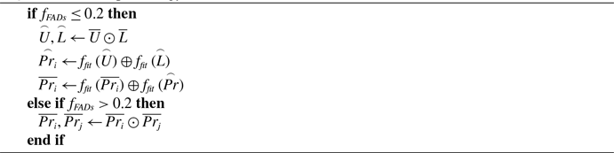
 \begin{equation} \begin{cases} & \overline {{Pr}_{t}}=\overline {{Pr}_{t}}\oplus best(\overrightarrow {U}\!\!\odot \! \!\overrightarrow {L}){\,\,\,\,}t\in R,f\le {{f}_{FADs}} \\ & \overline {{Pr}_{i}},\overline {{Pr}_{j}}= \overline {P{{r}_{i}}}\odot \overline {P{{r}_{j}}}{\,\,\,\,\,}i,j \in U, f\gt {{f}_{FADs}} \\ \end{cases} \end{equation}
where
 ${f}_{FADs}$
is a number with parameter
 $0.2$
,
 $f$
is a random number.
 $\overline {{Pr}_{i}}$
denotes the current prey population.
 $R$
is a set of random vectors, and
 $R\lt n$
,
 $r$
is the dimension of the
 $R$
vector.
 $\overrightarrow {U}$
is the worst result in the current search phase,
 $\overrightarrow {L}$
is the optimal result in the current search phase.
 $U$
is the selection of two prey items from all the prey items using the roulette pair method,
 $best()$
is the function that selects the sequence with the highest fitness value from
 $\overrightarrow {U}$
and
 $\overrightarrow {L}$
.
This equation indicates that when
 $f\le {{f}_{FADs}}$
, the process involves exchanging information with both the optimal and worst positions stored in oceanic memory. After this exchange, a decision is made on whether to accept the new position. If accepted, the position of a randomly selected prey is replaced; if not, no replacement occurs. Conversely, when
 $ f\gt {{f}_{FADs}}$
, two prey from the group are selected through the roulette method to exchange information and adopt the new position of the prey. As shown in Algorithm 4, it is the simplified pseudocode for this escape local optima strategy.
Escape strategy

Algorithm 4 Long description
An equation describing a conditional process for exchanging information between positions. The equation starts with a conditional statement: if f is less than or equal to f sub F A D s, then perform a series of operations. First, U hat and L hat are set to the union of U and L. Next, P r sub i is set to f sub j sub t of U hat combined with f sub j sub t of L. Then, P r sub i is set to f sub j sub t of P r sub i combined with f sub j sub t of P r sub i hat. If f is greater than f sub F A D s, then P r sub i and P r sub j are set to P r sub i and P r sub j combined with P r sub i and P r sub j. The equation ends with an end if statement.
4.4. Updating of the sea area
In seas with pheromones, predator updates, environmental adjustments, and leader individual updates are required.
Predator update: In the prey group, find the prey with the best current position and promote it to predator.
Environment update: A greedy mechanism is used to update the environment. If a new predator is found, the environment is updated according to Eq. (4).
4.5. Algorithmic process
At the beginning of the NMPA, the following parameters need to be set: population size
 $n$
, pheromone factor
 $\alpha$
, heuristic factor
 $\beta$
, the quantity parameter of selecting cities in Brownian Motion with pheromone
 $w$
, number of times of prey searching
 $p$
in each cycle, the maximum number of iterations
 ${t}_{max}$
, and the rate of evaporation
 $\rho$
. The pheromone factor
 $\alpha$
typically takes values between [1, 5], indicating the degree of reliance on the already discovered paths. The heuristic factor
 $\beta$
is generally chosen in the range [2, 5], reflecting the algorithm’s reliance on prior knowledge. The parameter
 $w$
for selecting cities with pheromone-driven Brownian motion controls the balance between exploration and exploitation, and is selected based on the number of cities to ensure reasonable convergence speed and solution accuracy. The number of prey searching
 $p$
is adjusted according to the number of cities; the more cities, the higher the number of searches. The maximum number of iterations
 $t_{max}$
is also set according to the problem size, with larger numbers of cities requiring higher iteration limits. Finally, the evaporation rate
 $\rho$
is set in the range of [0.1, 0.5] to prevent premature convergence, with values chosen based on the specific problem. As shown in Figure 6 shows the flowchart of the NMPA.
In terms of time complexity, the NMPA algorithm performs a total of
 $t_{max}$
iterations, with each iteration requiring the handling of
 $n$
prey and predators. For each prey and predator, operations such as Brownian motion, pheromone updates, and 2-opt/3-opt typically have a complexity of
 $O(n)$
, where
 $n$
is the number of cities in the TSP problem, or the number of tasks in the robot task allocation problem. The complexity of operations in each phase (exploration, exploitation, etc.) increases linearly with the population size
 $n$
. Therefore, the total time complexity of the algorithm is approximately
 $O(t_{max} \cdot n)$
.
In terms of space complexity, the algorithm needs to store the positions of
 $n$
prey and
 $n$
predators, as well as their corresponding pheromone values. This requires
 $O(n)$
space to store the positions and pheromone values. Therefore, the space complexity is also
 $O(n)$
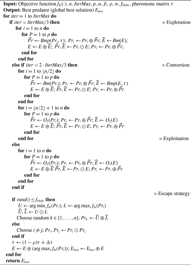
. The Algorithm 5 presents the pseudocode for the NMPA algorithm.
NMPA (Novel marine predator algorithm)

Algorithm 5 Long description
An equation describing the space complexity of an algorithm. The equation states that the algorithm needs to store the positions of n prey and n predators, as well as their corresponding pheromone values. This requires O of n space to store the positions and pheromone values. Therefore, the space complexity is also O of n.
The flowchart of NMPA.

5. Experiments and analysis of results
To comprehensively evaluate the performance of the proposed algorithm in robot task allocation, a series of experiments is conducted from three complementary perspectives:
-
1. Evaluation of search capability: To fundamentally analyze the search performance of the proposed NMPA, the TSPLIB benchmark library is adopted. This experiment investigates the impact of population size and compares the proposed algorithm with both conventional and advanced improved metaheuristics.
-
2. Single-robot task allocation with hard time windows: The NMPA is applied to a single-robot scheduling model constrained by hard time windows. Its optimization performance is compared with three representative algorithms: ant ccolony optimization (ACO) [Reference Skinderowicz30], simulated annealing (SA) [Reference Shi, Wu, Jiang and Karimi31], genetic algorithm (GA) [Reference Sohail32], particle swarm optimization(PSO) [Reference Tijjani, Wahab and Noor33], snow geese algorithm(SGA) [Reference Tian, Liu and Lv34], and MPA.
-
3. Multi-robot task allocation: The NMPA is further extended to a multi-robot task allocation model. First, standard datasets-MTSP-51, MTSP-100, and MTSP-150–are employed to evaluate its scalability and convergence behavior. Subsequently, comparative experiments with existing algorithms are performed to assess relative performance. Finally, a real-world multi-robot allocation case study is carried out to validate the practicality and efficiency of the proposed approach in realistic scenarios.
All experiments were conducted in a Python 3.8 environment on a Windows 11 operating system, running on an Intel(R) Core(TM) i7-8550U processor with 8 GB RAM. To ensure a fair comparison, the parameters of all baseline algorithms were configured according to the recommended settings reported in their original literature.
5.1. Experiment 1
5.1.1. TSP mathematical description
In the DFJ formulation, a TSP can be represented by an assignment-complete graph
 $G = (V, E)$
, where
 $V$
denotes the vertex set and
 $E$
denotes the edge set. The distance between vertices
 $i$
and
 $j$
is denoted as
 $d _ { i, j }$
and is assumed to be known. To represent the TSP mathematically, we introduce a binary decision variable
 $x _ { ij }$
, where
 $x _ { ij } = 1$
if the cyclic path contains the edge
 $(i, j)$
and
 $x _ { ij } = 0$
otherwise. The goal is to minimize the total distance traveled, which can be expressed as:
 \begin{equation} \min Z=\sum \limits _{i=1}^{n}{\sum \limits _{j=1}^{n}{{{d}_{ij}}{{x}_{ij}}}} \end{equation}
Subject to the following restrictions
Each city must be visited exactly once:
 \begin{equation} s.t.\text{ }\sum \limits _{j=1}^{n}{{{x}_{ij}}=1\text{ }i}\in V \end{equation}
Each city must be left exactly once:
 \begin{equation} \,\,\,\,\,\,\,\sum \limits _{i=1}^{n}{{{x}_{ij}}=1\text{ }j}\in V \end{equation}
Subtour elimination constraints to prevent subtours:
 \begin{equation} \,\,\,\,\,\,\,\underset {i\in S}{\mathop {\sum }}\,\underset {j\in S}{\mathop {\sum }}\,{{x}_{ij}}\le |S|-1,\forall S\subset V,2\le |S|\le n-1 \end{equation}
 \begin{equation} \,\,\,\,\,\,\,{{x}_{ij}}\in \{0,1\},i,j\in V, \end{equation}
5.1.2. TSP example test
In the context of the TSP, the accuracy of an algorithm’s solution is typically evaluated using two types of errors:
 \begin{equation} PD=\frac {\sum \limits _{K=1}^{T}{(\text{bes}{{\text{t}}_{\text{k}}}-{{S}_{0}})}}{T\times {{S}_{0}}}\times 100 \end{equation}
 \begin{equation} BSE=\frac {BEST-{{S}_{0}}}{{{S}_{0}}}\times 100 \end{equation}
where
 $\text{best}$
is the algorithm used to solve to the optimal path,
 ${S}_{0}$
is the shortest path value provided by TSPLIB, and
 $T$
is the number of times the experiment was tested.
 $PD$
denotes the average of the optimal path result values obtained after
 $T$
experiments, and
 $BEST$
is the best result of the optimal path result values obtained after
 $T$
experiments.
 $BSE$
is the error of the best result of the optimal path result value obtained after
 $T$
experiments.
(1) Experiments on population size change
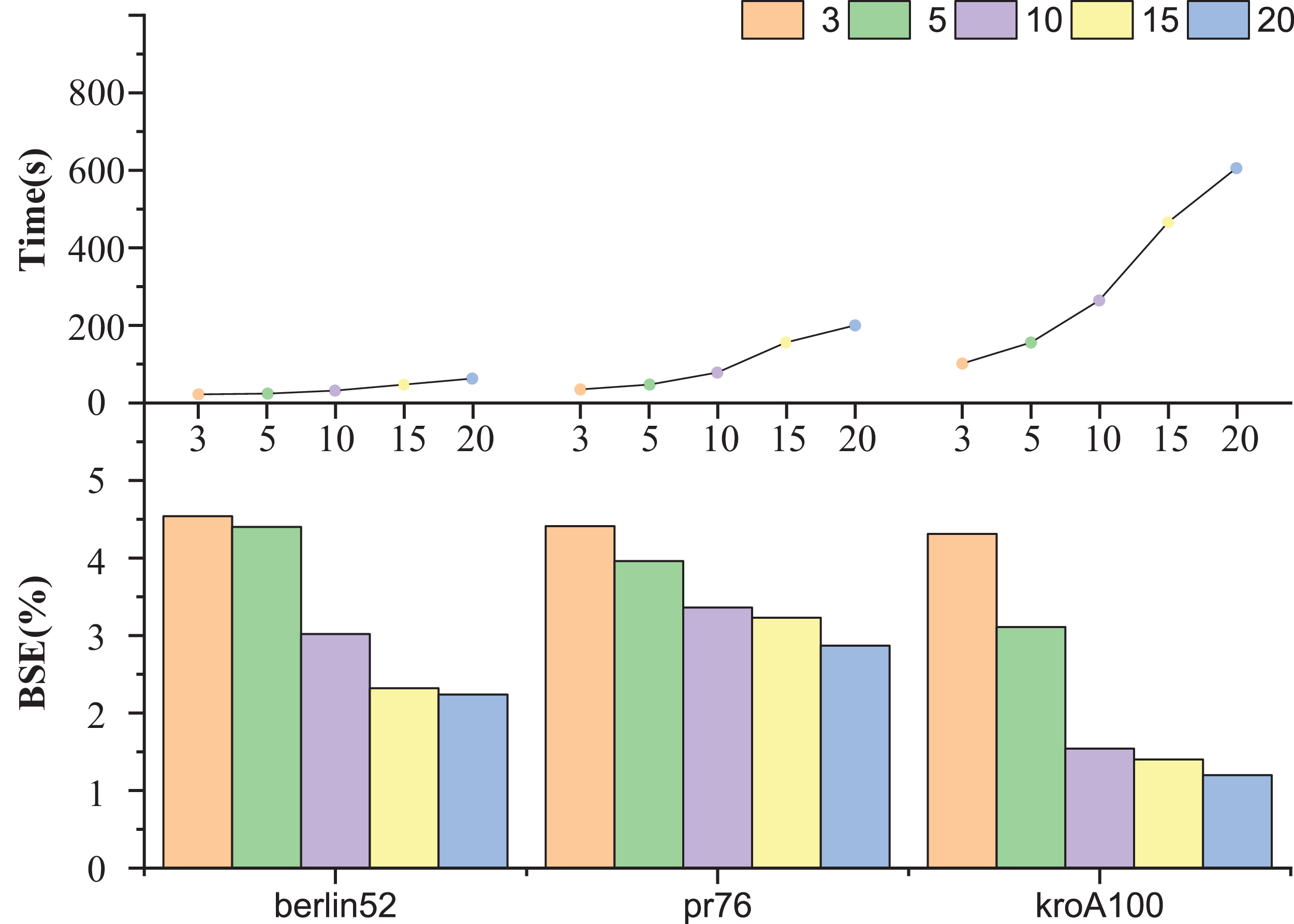
Unlike traditional algorithms such as PSO, GAs, and ant colony optimization, NMPA distinguishes itself by not limiting its populations to exploring only in the same direction. Instead, each population in the NMPA explores a new direction. Once all populations have explored their respective directions, the optimal population is selected as the predator, ensuring that each direction explored is effective. To investigate the impact of changes in population size, three TSP instances are utilized: berlin52, pr76, and kroA100. To maintain consistency in the comparison of experimental results, only the number of populations is varied, while other relevant parameters are kept constant, as detailed below:
berlin52:
 $\alpha =5$
,
 $\beta =4$
,
 $p=100$
,
 $w=10$
,
 $t_{max}=100$
,
 $\rho =0.5$
pr76:
 $\alpha =5$
,
 $\beta =4$
,
 $p=200$
,
 $w=15$
,
 $t_{max}=100$
,
 $\rho =0.5$
kroA100:
 $\alpha =5$
,
 $\beta =4$
,
 $p=300$
,
 $w=15$
,
 $t_{max}=150$
,
 $\rho =0.5$
The population sizes used are 3, 5, 10, 15, and 20, as shown in Figure 7. where the top of the picture shows the effect of the population change on time, with the result being the average of the time it took to run out the result after solving it 30 times using the NMPA. The lower part of the picture shows the effect of the change in population on the accuracy of the solution, the result of which is the error in the average value of the time to run out the optimal solution after solving the problem 10 times using the NMPA. From Figure 7, it can be seen that the higher the population size of the prey, the more accurate the NMPA is, but the length of time required increases.
Impact of population changes on the results of NMPA.

Figure 7 Long description
The image contains two graphs: a line graph and a bar graph. The line graph at the top shows the time taken for task execution by robots across different scenarios. The x-axis represents different task points labeled as 3, 5, 10, 15, and 20, while the y-axis represents the time taken in seconds. The line graph includes data points for three different task scenarios: berlin52, pr76, and kroA100, each represented by different colors. The time taken increases as the number of task points increases, with the highest time observed at 20 task points. The bar graph at the bottom shows the benefit of task execution (BSE percent) for the same scenarios. The x-axis represents the different task scenarios (berlin52, pr76, and kroA100), and the y-axis represents the BSE percent. Each scenario is represented by bars of different colors corresponding to the number of task points (3, 5, 10, 15, and 20). The BSE percent decreases as the number of task points increases, with the highest BSE percent observed at 3 task points. The combination of these graphs illustrates the trade-off between time taken and benefit of task execution as the number of task points increases.
(2) Experiments comparing NMPA with other algorithms
To understand the performance of the algorithm, the NMPA is utilized to solve 20 sets of TSP instances 30 times, and the related results are recorded. The parameter settings of NMPA is: population size
 $n=6$
, pheromone factor
 $\alpha =5$
, heuristic factor
 $\beta =4$
, the rate of evaporation
 $\rho$
, the parameter of the number of cities selected with Brownian Motion with pheromone
 $w$
, The maximum number of iterations
 ${t}_{max}$
and the number of prey searches per cycle
 $p$
need to be fine tuned according to the actual situation.
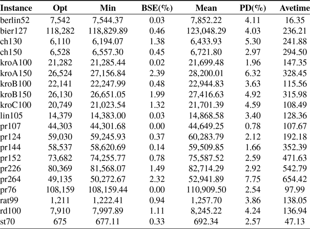
Table I presents the results obtained from solving the TSP instances using the NMPA. The metrics used to evaluate the performance include PD and BES. In Table I,
 $Opt$
is the shortest path value provided by TSPlib,
 $Min$
is the best result out of 10 solvers, and
 $Mean$
is the average value of the results obtained from 10 solvers.
 $Avetime$
is the average value of the solution time for the solution of 10 times that yields the optimal result. From Table I and Figure 8, it can be seen that the results of NMPA solving converge to a certain good range.
Solution results for 20 sets of TSP instances.

Table I Long description
A table comparing solution results for 20 sets of TSP instances. The table has 20 rows and 6 columns. The columns are labeled Instance, Opt, Min, BSE(percent), Mean, PD(percent), and Avetime. Each row represents a different TSP instance with corresponding values for each metric. Row 1: Instance, berlin52; Opt, 7.542; Min, 7.544.37; BSE(percent), 0.03; Mean, 7.852.22; PD(percent), 4.11; Avetime, 16.35. Row 2: Instance, eil127; Opt, 118.282; Min, 118.829.89; BSE(percent), 0.46; Mean, 123.048.29; PD(percent), 4.03; Avetime, 236.21. Row 3: Instance, ch130; Opt, 6.110; Min, 6.194.07; BSE(percent), 1.38; Mean, 6.433.93; PD(percent), 5.30; Avetime, 241.88. Row 4: Instance, ch150; Opt, 6.528; Min, 6.557.30; BSE(percent), 0.45; Mean, 6.721.80; PD(percent), 2.97; Avetime, 294.50. Row 5: Instance, kroA100; Opt, 21.282; Min, 21.285.44; BSE(percent), 0.02; Mean, 21.699.48; PD(percent), 1.96; Avetime, 147.35. Row 6: Instance, kroA150; Opt, 26.524; Min, 27.156.84; BSE(percent), 2.39; Mean, 28.200.01; PD(percent), 6.32; Avetime, 328.45. Row 7: Instance, kroB100; Opt, 22.141; Min, 22.247.99; BSE(percent), 0.48; Mean, 22.944.83; PD(percent), 3.63; Avetime, 115.56. Row 8: Instance, kroB150; Opt, 26.130; Min, 26.651.05; BSE(percent), 1.99; Mean, 27.416.63; PD(percent), 4.92; Avetime, 315.98. Row 9: Instance, kroC100; Opt, 20.749; Min, 21.023.54; BSE(percent), 1.32; Mean, 21.701.39; PD(percent), 4.59; Avetime, 108.49. Row 10: Instance, lin105; Opt, 14.379; Min, 14.383.00; BSE(percent), 0.03; Mean, 14.868.58; PD(percent), 3.40; Avetime, 128.36. Row 11: Instance, pr107; Opt, 44.303; Min, 44.301.68; BSE(percent), 0.00; Mean, 44.649.25; PD(percent), 0.78; Avetime, 10.76. Row 12: Instance, pr124; Opt, 59.030; Min, 59.245.93; BSE(percent), 0.37; Mean, 60.283.79; PD(percent), 2.12; Avetime, 192.18. Row 13: Instance, pr144; Opt, 58.537; Min, 58.620.69; BSE(percent), 0.14; Mean, 59.509.85; PD(percent), 1.66; Avetime, 352.39. Row 14: Instance, pr152; Opt, 73.682; Min, 74.255.77; BSE(percent), 0.78; Mean, 75.587.52; PD(percent), 2.59; Avetime, 471.63. Row 15: Instance, pr226; Opt, 80.369; Min, 81.568.07; BSE(percent), 1.49; Mean, 82.714.29; PD(percent), 2.92; Avetime, 542.79. Row 16: Instance, pr264; Opt, 49.135; Min, 50.272.67; BSE(percent), 2.32; Mean, 52.941.89; PD(percent), 7.75; Avetime, 654.42. Row 17: Instance, pr76; Opt, 108.159; Min, 108.159.44; BSE(percent), 0.00; Mean, 110.909.50; PD(percent), 2.54; Avetime, 97.99. Row 18: Instance, rat78; Opt, 1.211; Min, 1.222.41; BSE(percent), 0.94; Mean, 1.257.70; PD(percent), 3.86; Avetime, 138.05. Row 19: Instance, rl1304; Opt, 7.910; Min, 7.997.89; BSE(percent), 1.11; Mean, 8.245.22; PD(percent), 4.24; Avetime, 136.94. Row 20: Instance, st70; Opt, 675; Min, 677.11; BSE(percent), 0.33; Mean, 692.34; PD(percent), 2.57; Avetime, 47.13.
Partial solution results of TSP instances.

Figure 8 Long description
The image contains six line graphs, each representing partial solution results of different traveling salesman problem (TSP) instances. Each graph shows a path connecting various points, illustrating the route taken to solve the TSP. Panel A, labeled berlin52, displays a line graph with axes ranging from 0 to 1750 on the x-axis and 0 to 2000 on the y-axis. The path forms a closed loop without subloops, connecting multiple points. Panel B, labeled ch130, shows a line graph with axes ranging from 0 to 700 on the x-axis and 0 to 700 on the y-axis. The path is more complex, with multiple intersections and a closed loop. Panel C, labeled kroA100, depicts a line graph with axes ranging from 0 to 4000 on the x-axis and 0 to 2000 on the y-axis. The path is intricate, connecting numerous points in a closed loop. Panel D, labeled kroA150, shows a line graph with axes ranging from 0 to 4000 on the x-axis and 0 to 2000 on the y-axis. The path is highly complex, with many intersections and a closed loop. Panel E, labeled pr76, displays a line graph with axes ranging from 0 to 20000 on the x-axis and 0 to 12000 on the y-axis. The path is extensive, connecting multiple points in a closed loop. Panel F, labeled pr107, shows a line graph with axes ranging from 8000 to 16000 on the x-axis and 5000 to 11000 on the y-axis. The path is vertical, connecting points in a straight line. Each graph illustrates the solution to a TSP instance, demonstrating the complexity and variability of the problem.
Comparison results between NMPA and traditional algorithms.

Table II Long description
The table compares the performance of various algorithms across four datasets: berlin52, pr76, kroA100, and pr107. The table has 8 rows and 13 columns. The columns are labeled as follows: Algorithm, BSE (%), PD (%), Time, BSE (%), PD (%), Time, BSE (%), PD (%), Time, BSE (%), PD (%), Time. The rows are labeled with the names of the algorithms: ACO, SA, GA, PSO, SGA, MPA, NMPA. Each row provides the values for BSE (%), PD (%), and Time for each dataset. Row 1: ACO, 3.45, 8.43, 129.35, 10.79, 14.37, 405.72, 13.62, 17.10, 1,055.44, 7.24, 9.72, 1972.25. Row 2: SA, 2.84, 8.49, 46.51, 3.93, 12.18, 70.17, 9.27, 17.20, 112.68, 3.16, 9.55, 131.96. Row 3: GA, 0.03, 6.14, 18.10, 1.74, 3.58, 56.87, 0.43, 2.19, 122.04, 0.54, 0.95, 156.80. Row 4: PSO, 1.00, 6.74, 12.15, 12.04, 16.89, 32.93, 11.02, 14.38, 66.55, 1.84, 2.80, 72.44. Row 5: SGA, 0.31, 5.01, 16.99, 5.83, 3.47, 40.55, 1.15, 2.14, 99.79, 0.99, 0.91, 101.19. Row 6: MPA, 0.54, 5.21, 17.45, 8.11, 9.91, 98.17, 9.02, 10.47, 149.87, 0.89, 1.67, 108.79. Row 7: NMPA, 0.03, 4.11, 16.35, 0.00, 2.54, 97.99, 0.02, 1.96, 147.35, 0.00, 0.78, 107.67.
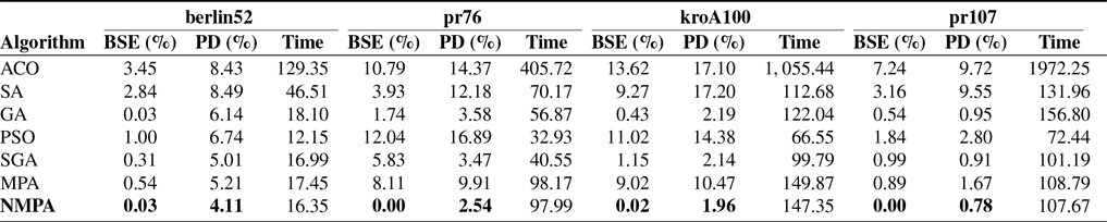
To gain a deeper insight into the performance of NMPA, NMPA is compared with several traditional algorithms, including ACO, SA, GA, PSO, SGA, and MPA. Each algorithm was tasked with performing 30 optimization solutions on four TSP instances: Berlin52, pr76, kroA100, and pr107. The results of these comparisons are presented in Table II. In the Table II, it is evident that NMPA achieves better results than the traditional algorithms in BSE and Min, demonstrating its high optimization accuracy and robustness.
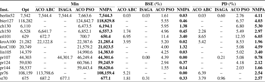
To evaluate the effectiveness of the NMPA relative to other methods reported in the literature, comparisons were conducted with various hybrid and advanced algorithms such as ACO-ABC, ISAGA, and ACO-PSO. These algorithms are referenced in [Reference Gündüz, Kiran and Özceylan35–Reference Qian and Su37]. The results of these comparisons are detailed in Table III. The comparison is based on evaluation metrics such as BSE, PD, and Min. From the data in Table III, it is apparent that the NMPA outperforms the compared algorithms in terms of both results and accuracy when solving TSP. Additionally, the algorithm demonstrates an ability to converge within a high-quality range. (In table III, “-” indicates that the result is not mentioned in the literature, and the bold part represents the solution result of the NMPA.)
Comparison results between NMPA and other algorithms.

Table III Long description
A table comparing performance metrics of different algorithms. The table has 14 rows and 15 columns. The columns are labeled as Inst., Opt, Min, BSE (%), and PD (%), with sub-columns for ACO ABC, ISAGA, ACO PSO, and NMPA under Min, BSE (%), and PD (%). The rows are labeled with instance names such as berlin52, bier127, ch130, and so on. Each cell contains numerical values representing the performance metrics of the algorithms. Notable trends include varying performance across different instances and algorithms, with some instances showing significant differences in metrics. The table provides a detailed comparison of the effectiveness of NMPA against other algorithms like ACO-ABC, ISAGA, and ACO-PSO.
5.2. Experiment 2
5.2.1. Mathematical description of task assignment for a single robot
Based on the practical requirements of modern factory production lines, where robots are tasked with materials handling and assembly operations within fixed timeframes to maximize operational efficiency, a specific model of the TSP with hard time windows is formulated. This problem scenario encompasses several key characteristics:
-
1. The location of the robot’s charging pile and the task point is known.
-
2. The lossness that needs to be referenced between each task point and the robot’s charging pile is known, such as path length, moving speed, working time, service time, and so on.
-
3. The path during the task process starts with the robot’s charging pile, and it needs to return to the charging pile after completing all the tasks to form a closed-loop line.
-
4. Each task point has and can only be reached once.
-
5. The influence of obstacle factors on the robot is not considered.
Based on the above problem description, a specific model of the TSP with hard time windows is established, and the problem is described as follows.
Parameter settings:
-
$N$
is the total number of task points, including charging pile and task points,
-
$i, j$
are the index of the task point,
$i, j = 1, 2, \ldots , N$
,
-
$d_{ij}$
is distance or cost from task point
$i$
to task point
$j$
,
-
$e_i$
is the start time of the time window for task point
$i$
,
-
$l_i$
is the end time of the time window for task point
$i$
,
-
$ {t}_ {i}$
is access time of task point
$i$
.





Decision variables:
-
$x_{ij}$
is a binary variable that takes the value 1 when the robot moves from task point
$i$
to task point
$j$
, and 0 otherwise.


Objective function:
 \begin{equation} \min \sum _{i=1}^{N} \sum _{j=1,\, j \neq i}^{N} d_{ij} \cdot x_{ij} \end{equation}
Constraints:
(1) Each task point must be visited by the robot exactly once and the robot may visit it only once:
 \begin{equation} \begin{aligned} &\sum _{j=1,\, j \neq i}^{N} x_{ij} = 1, \quad \forall i = 1, 2, \ldots , N\\ &\sum _{i=1,\, i \neq j}^{N} x_{ij} = 1, \quad \forall j = 1, 2, \ldots , N \end{aligned} \end{equation}
(2) The robot’s path must begin and end at the charging post:
 \begin{equation} \begin{aligned} &\sum _{j=2}^{N} x_{1j} = 1\\ &\sum _{i=2}^{N} x_{i1} = 1 \end{aligned} \end{equation}
(3) The duration of each mission point visit must fall within the time window:
 \begin{equation} e_j \leq \sum _{i=1}^{N} x_{ij} \cdot t_i \leq l_j, \quad \forall j = 2, 3, \ldots , N \end{equation}
(4) Decision variables must be binary:
 \begin{equation} x_{ij} \in \{0, 1\}, \forall i = 1, 2, \ldots , N \forall j = 1, 2, \ldots , N \end{equation}
By solving this model, optimal robot work routes that satisfy the time-window constraints can be obtained to reduce the transportation cost and comply with the time constraints.
5.2.2. Example experiments with a single robot
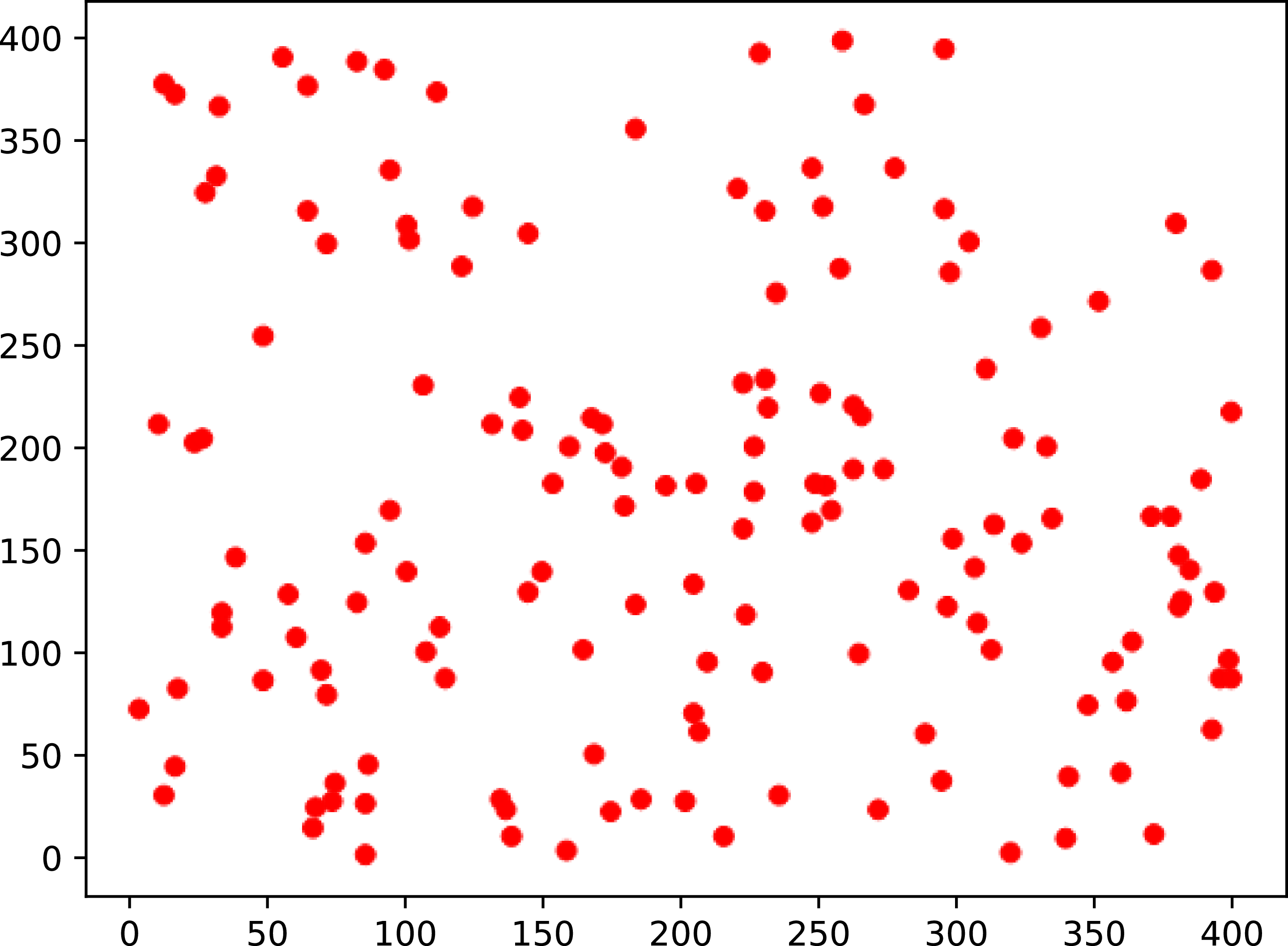
The dataset related to a factory handling robot task is presented in Table VIII, which contains a total of 153 records. Each record specifies the coordinates of a task point, the required service (demand) time, and the corresponding service interval. The demand time refers to the duration required for the robot to complete the assigned task at a specific point, whereas the service interval defines the time window during which the robot must arrive at the task point; the robot is not allowed to visit the point outside this interval. The robot operates at a constant speed of 5 m/min. The spatial distribution of the 153 task points is illustrated in Figure 9.
The distribution of 153 task points.

Heuristic algorithms often begin with random populations, which can be a challenge in models like the model of the TSP with hard time windows, where the task constraints don’t fit for random initial solutions. However, optimization algorithms can be used to initialize each population. In this process, each algorithm is first used to generate initial solutions that adhere to the hard time window constraints. These initial solutions are then further optimized using their respective algorithms to effectively address the robot’s hard time-window model. The primary optimization goal for each algorithm is to maximize the number of tasks that comply with the hard time-window constraints. Once all task points in a solution meet their respective time windows, this solution set is added to the population. This addition continues until the required initial population size for the algorithm is reached.
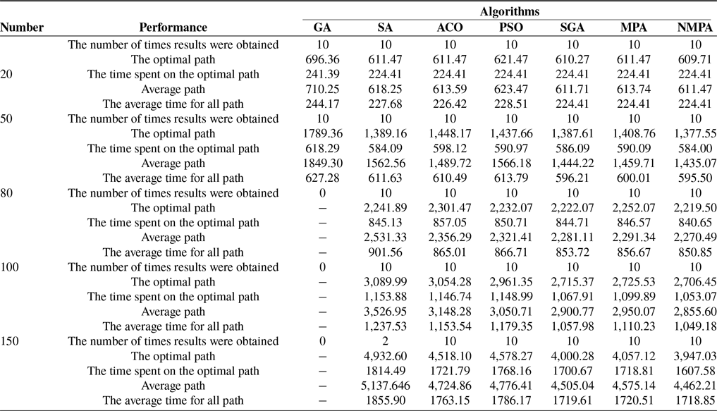
Experimental arrangement: to understand more about the performance of NMPA to solve the robot task allocation model for single robot, so the above task points are taken out the first 20 task points as a set of robot task requirements, and the same get 50 task requirements, 80 task requirements, 100 task requirements, and 150 task requirements. GA, SA, ACO, PSO, SGA, MPA, and NMPA are used to solve each task requirement 10 times, and the solved results are shown in Table IV. In Table IV, The number of times results were obtained is the number of times the result can be obtained by 10 times of solving, The optimal path is the best result among the optimization results obtained by the algorithm, The time spent on the optimal path is the time spent on the robot to traverse all the task points in accordance with the sequence of optimal paths obtained by the algorithm, Average path is the average of all the values of the number of times the algorithm obtains the result, The average time for all path is the average of the sum of the time spend on the robot to traverse the sequence of path solved by the algorithm each time. The parameter settings for ACO, SA, GA, PSO, SGA, MPA, and NMPA are as follows:
Solution results of NMPA and traditional algorithms for the man-robot problem.

Table IV Long description
A table comparing the performance of various algorithms for solving the man-robot problem. The table has 7 columns and 15 rows, including headers. The columns are labeled as follows: Number, Performance, GA, SA, ACO, PSO, SGA, MPA, and NMPA. The rows are labeled with different performance metrics and the number of task requirements (20, 50, 80, 100, 150). Each cell contains numerical values representing the performance of each algorithm under different conditions. The table provides detailed data on the number of times results were obtained, the optimal path, the time spent on the optimal path, the average path, and the average time for all paths. Notable trends include the varying performance of different algorithms across different task requirements, with some algorithms consistently outperforming others in terms of optimal path and time spent.
Relevant parameters of ACO: pheromone factor 1, heuristic factor 5, population size 200, evaporation rate 0.5, number of iterations 300.
Parameters related to the SA: start temperature 10, end temperature 0.1, number of cycles 500, coefficient of cooling 0.998.
Relevant parameters of the GA: selection rate 0.5, mutation rate 0.35, population size 800, number of iterations 800.
The relevant parameters of PSO: population size is 200, maximum number of iterations is 800. A random-key encoding is used to map particle positions to visiting sequences, where the position values are bounded in
 $[0,1]$
and any out-of-bounds values are handled by clipping. The inertia weight
 $w$
follows a linearly decreasing strategy with
 $w_{\max }=0.9$
and
 $w_{\min }=0.4$
, and the learning factors are set to
 $c_1=c_2=2.0$
.
The relevant parameters of SGA: the population size is 200, and the maximum number of iterations is 800. A random-key encoding is adopted to map snow-goose positions into visiting sequences, where the position values are bounded in
 $[0,1]$
and any out-of-bound values are handled by the clipping operation. In the exploration stage, the control coefficient
 $c$
is computed by
 $c=\frac {4t}{M\cdot e^{4t/M}}$
, and the velocity is updated via
 $V^{t+1}=c\cdot V^t+a$
. The random coefficients
 $b$
and
 $d$
are generated from a uniform distribution in
 $(0,1)$
, and the position is updated by
 $P_i^{t+1}=P_i^{t}+b\cdot (P_b^{t}-P_i^{t})-d\cdot (P_c^{t}-P_i^{t})+V_i^{t+1}$
. In the exploitation stage, the position is updated according to the straight-line flight strategy, and a Brownian perturbation is introduced when
 $r\le 0.5$
, where
 $r\sim U(0,1)$
.
Relevant parameters of the MPA: population size
 $n=6$
, number of times of prey searching
 $p=500$
in each cycle, and the maximum number of iterations
 ${t}_{max}=300$
.
Relevant parameters of the NMPA: population size
 $n=6$
, pheromone factor
 $\alpha =3$
, heuristic factor
 $\beta =7$
, the quantity parameter of selecting cities in Brownian Motion with pheromone
 $w=15$
, number of times of prey searching
 $p=500$
in each cycle, the maximum number of iterations
 ${t}_{max}=300$
, and the rate of evaporation
 $\rho =0.5$
.
From Table IV, the proposed NMPA can stably obtain feasible solutions for all problem scales, and its optimal and average paths remain the best or close to the best overall, demonstrating good convergence and robustness. Figure 10 shows the optimal results obtained by the NMPA algorithm described in this paper for various examples. In contrast, the ability of conventional algorithms to generate feasible solutions under hard time-window constraints differs significantly: GA can obtain solutions only in the 20- and 50-task scenarios, while its success count drops to zero when the number of task points is greater than or equal to 80; SA obtains feasible solutions only 2 out of 10 runs in the 150-task scenario, indicating insufficient capability in constructing initial feasible solutions and exploring within the feasible region under strict time-window constraints. Further comparison of solution quality shows that, in the 100-task instance, the optimal path length of NMPA is 2,706.45, which is reduced by 12.41%, 11.39%, and 8.61% compared with SA/ACO/PSO, respectively, and it also outperforms similar swarm-intelligence algorithms, SGA and MPA. In the 150 task instances, the optimal path length of NMPA is 3,947.03, which is reduced by 19.98%, 12.64%, and 13.79% compared with SA, ACO, PSO, respectively, and it further outperforms SGA and MPA, with a larger advantage. In terms of stability, the average path lengths of NMPA are 2,855.60 and 4,462.21 for the 100 and 150 task scenarios, respectively, which are reduced by 6.40% and 6.58% compared with PSO, and the average solutions are closer to the corresponding optimal solutions, indicating smaller performance fluctuations and more stable convergence. During the experiments, it was observed that the hard time-window model requires the arrival service time at each task point along the route to strictly satisfy the time constraints; this requirement tends to prevent heuristic algorithms from generating feasible routes during initialization or iteration, leading to failures in obtaining solutions. Taking ACO as an example, it relies on pheromone guidance and candidate-node filtering, which can prioritize task points satisfying the time-window constraints to some extent and thus maintain feasibility; however, due to the lack of stronger global guidance and diversity-preservation mechanisms, it is still prone to falling into local optima. By contrast, NMPA incorporates pheromone-guided Brownian motion and adopts a roulette-wheel strategy to actively screen task points that satisfy the hard time-window requirements, resulting in more reasonable visiting sequences and easier feasibility preservation; consequently, it can maintain stable solving capability and achieve superior path results under large-scale and strict time-window conditions. Overall, these results indicate that the proposed NMPA not only improves solution quality and stability but also achieves superior convergence efficiency, especially in large-scale and hard time-window-constrained scenarios.
5.3. Experiment 3
5.3.1. Mathematical description of a multi-robot task allocation model
According to the actual unmanned factory, there is not only the task assignment of single robots but also the multi-robot mutual collaboration. Therefore, in order to test the application of this paper’s algorithm in multi-robot systems, the NRTA description is constructed based on the multi-robot intelligent autonomous task execution scenario with the performance index minimization as the objective function. In the actual multi-robot task allocation, there are the following basic scenarios: the number of robot tasks is much larger than the number of robots, each robot is required to execute multiple robot tasks, and each task can be executed by only one robot. Based on the above problem description, a model with multiple robots is developed with the following problem description:
Parameter settings:
-
$Z$
is the total cost for the robot to complete all tasks,
-
$N$
is the set of robots
$N=\left \{ {{n}_{1}},{{n}_{2}},\cdots {{n}_{k}}\cdots {{n}_{t}} \right \}$
, where
$t$
is the total number of robots,
-
$M$
is the index of the task,
$M= \left \{{ {{m}_{1}}}, {{m}_{2}} ,\cdots {{m}_{r}} \right \}$
, where
$r$
is the total number of tasks,
-
$W$
is the position index of the robot
$W=\left \{ {{W}_{1}},{{W}_{2}},\cdots {{W}_{t}} \right \}$
,
-
$x_{ij}^{k}$
is decision variable indicating that the robot
${n}_{k}$
arrives at task
${m}_{j}$
from task
${m}_{i}$
. If the operation is performed then
$x_{ij}^{k}=1$
, otherwise
$x_{ij}^{k}=0$
,
-
$y_{j}^{k}$
is decision variable indicating that the robot
${n}_{k}$
visits the task node
${m}_{j}$
. If the operation is performed then
$y_{j}^{k}=1$
, otherwise
$y_{j}^{k}=0$
,
-
${g}_{ij}$
is the cost from task
${m}_{i}$
to task
${m}_{j}$
,











The distribution of 150 task points.

Figure 10 Long description
Panel A: A line graph shows the distribution of 20 mission points. The x-axis ranges from 320 to 400, and the y-axis ranges from 0 to 200. The graph features red dots connected by blue lines, indicating the mission points. Panel B: A line graph displays the distribution of 50 mission points. The x-axis ranges from 100 to 400, and the y-axis ranges from 0 to 200. The graph includes red dots connected by blue lines, with a star marker indicating a specific point. Panel C: A line graph illustrates the distribution of 80 mission points. The x-axis ranges from 0 to 400, and the y-axis ranges from 0 to 400. The graph features red dots connected by blue lines, with a star marker indicating a specific point. Panel D: A line graph shows the distribution of 100 mission points. The x-axis ranges from 0 to 400, and the y-axis ranges from 0 to 400. The graph includes red dots connected by blue lines, with a star marker indicating a specific point. Panel E: A line graph depicts the distribution of 150 mission points. The x-axis ranges from 0 to 400, and the y-axis ranges from 0 to 400. The graph features red dots connected by blue lines, with a star marker indicating a specific point.
Objective function:
 \begin{equation} \min Z=\sum \limits _{i=1}^{M+W}{\sum \limits _{j=1}^{M+W}{{{g}_{ij}}}}x_{ij}^{k} \end{equation}
Constraints:
-
(1) It is required that each task will be assigned to only one robot for execution:
(31)
\begin{equation} \sum \limits _{k=1}^{m}{y_{i}^{k}}=1,i=m+1,m+2,\ldots ,m+n \end{equation}
-
(2) The sum of the number of tasks performed by all robots is required to be equal to the total number of tasks received:
(32)
\begin{equation} \sum \limits _{i=M+1}^{M+W}{\sum \limits _{k=1}^{M}{y_{i}^{k}}}=n \end{equation}
-
(3) Require that only one predecessor node can pass through any one node:
(33)
\begin{equation} \sum \limits _{j=1}^{M+W}{x_{ij}^{k}}=y_{i}^{k}\text{ }j=m+1,m+2,\cdots ,M+N \end{equation}
-
(4) Require the next task that exists for every robot except the last task of each robot:
(34)
\begin{equation} \sum \limits _{j=1}^{M+W}{x_{ij}^{k}}=y_{i}^{k} \end{equation}


By solving this model, it is possible to obtain work routes that satisfy the collaboration of multiple robots in order to reduce transport costs.
5.3.2. Example 1
The form of the solution space for the multi-robots task allocation model can be encoded as an
 ${N+M-1}$
dimensional vector, where
 $N$
is the total number of robots and
 $M$
is the total number of tasks. Integers greater than M are used to denote different robot numbers, and the positive integer corresponding to each element of the vector denotes the task number or the different robot number splitting point. If the solution space of 3 robots performing 10 tasks is [1
 $\to$
2
 $\to$
3
 $\to$
11
 $\to$
4
 $\to$
5
 $\to$
6
 $\to$
7
 $\to$
12
 $\to$
8
 $\to$
9
 $\to$
10], then it means that, Robot 1 sequentially performs the tasks 1, 2, and 3. Robot 2 sequentially perform the tasks 4, 5, 6, and 7. Robot 3 sequentially performs tasks 8, 9, 10.
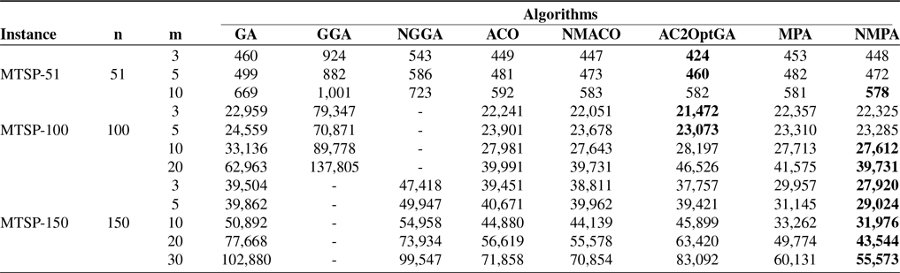
To evaluate the effectiveness of the proposed NMPA in multi-robot task allocation, experiments were conducted on multiple instances of the MTSP, specifically MTSP-51, MTSP-100, and MTSP-150. The obtained results were compared with those of several other algorithms, including the GGA and NGGA from the literature [Reference Singh, Singh, Singh and Prasad38], the NMACO from the literature [Reference Yousefikhoshbakht, Didehvar and Rahmati39], the AC2OptGA from the literature [Reference Harrath, Salman, Alqaddoumi, Hasan and Radhi40], as well as the traditional GA and ACO. Table V presents the comparison results in terms of the minimum path length for each instance, where
 $n$
denotes the number of tasks and
 $m$
represents the number of salesmen. The bolded values indicate the best results among the compared algorithms. The results show that the NMPA performs comparably to other algorithms in small-scale instances. However, as the problem scale and the number of salesmen increase, its superiority becomes more evident. Even for large-scale and complex cases such as MTSP-150, which demand strong global search capabilities, the NMPA demonstrates faster convergence and achieves better overall optimization performance than the other algorithms.
5.3.3. Example 2
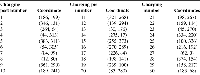
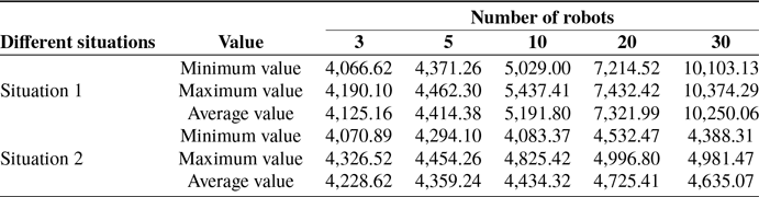
When multiple robots perform tasks in a storage environment, there are two aspects to the problem of facing charging piles: (1) Each robot has its own charging pile; thus, each robot starts from a different point and (2) all robots only have one charging pile; thus, each robot starts from the same point. Therefore, the 153 sets of task points in Appendix B and different numbers of robots (3, 5, 10, 20, 30) are utilized to test the performance of the NMPA to solve the above two situations. The coordinates of the charging piles of the robots for Situation 1 need to be selected sequentially from Table VI depending on the number of robots, and for Situation 2, all robots select the coordinates of the charging piles at the origin (0, 0) as the starting point.
As shown in Table VII, the results of the two situations solved by the NMPA are summarized. In Table VII, the Minimum value represents the shortest total path length of all robots following the best task sequence among ten independent runs of the NMPA, while the Maximum value denotes the longest total path length obtained under the worst task sequence. The Average value corresponds to the mean path length of all robots across the ten runs. As illustrated in Figure 11, for Situation 2, the results obtained by the NMPA converge to high-quality solutions, where the stars indicate the locations of the charging piles.
Results of NMPA and other algorithms for solving the MTSP-51, MTSP-100, and MTSP-150.

Table V Long description
A table comparing the performance of various algorithms on different instances of the Multiple Traveling Salesman Problem (MTSP). The table has 12 rows and 10 columns. The columns are labeled Instance, n, m, GA, GGA, NGGA, ACO, NMACO, AC2OptGA, MPA, and NMPA. The rows are labeled with different instances of MTSP (MTSP-51, MTSP-100, MTSP-150) and varying values of n and m. Each cell contains a numerical value representing the performance of the respective algorithm on the given instance. The table provides a detailed comparison of the algorithms' performance across different problem sizes and configurations.
Positioning coordinates of all charging posts.

Table VI Long description
The table presents the coordinates of charging posts, organized into three columns: Charging post number, Coordinate, and Charging pie number with Coordinate and Charging number. The table has 30 rows and 3 columns. Each row lists a charging post number, its corresponding coordinate, and the charging pie number with its coordinate and charging number. The data is presented as follows: Row 1: Charging post number 1, Coordinate (186, 199), Charging pie number 21, Coordinate (98, 267), Charging number 1. Row 2: Charging post number 2, Coordinate (346, 131), Charging pie number 12, Coordinate (139, 294), Charging number 2. Row 3: Charging post number 3, Coordinate (264, 64), Charging pie number 13, Coordinate (30, 176), Charging number 3. Row 4: Charging post number 4, Coordinate (44, 313), Charging pie number 14, Coordinate (275, 17), Charging number 4. Row 5: Charging post number 5, Coordinate (383, 311), Charging pie number 15, Coordinate (255, 373), Charging number 5. Row 6: Charging post number 6, Coordinate (54, 305), Charging pie number 16, Coordinate (270, 289), Charging number 6. Row 7: Charging post number 7, Coordinate (84, 99), Charging pie number 17, Coordinate (226, 84), Charging number 7. Row 8: Charging post number 8, Coordinate (12, 80), Charging pie number 18, Coordinate (198, 141), Charging number 8. Row 9: Charging post number 9, Coordinate (361, 290), Charging pie number 19, Coordinate (239, 100), Charging number 9. Row 10: Charging post number 10, Coordinate (189, 241), Charging pie number 20, Coordinate (85, 280), Charging number 10. Row 11: Charging post number 11, Coordinate (321, 268), Charging pie number 21, Coordinate (98, 267), Charging number 11. Row 12: Charging post number 12, Coordinate (139, 294), Charging pie number 22, Coordinate (159, 114), Charging number 12. Row 13: Charging post number 13, Coordinate (30, 176), Charging pie number 23, Coordinate (45, 270), Charging number 13. Row 14: Charging post number 14, Coordinate (275, 17), Charging pie number 24, Coordinate (334, 220), Charging number 14. Row 15: Charging post number 15, Coordinate (255, 373), Charging pie number 25, Coordinate (100, 336), Charging number 15. Row 16: Charging post number 16, Coordinate (270, 289), Charging pie number 26, Coordinate (216, 192), Charging number 16. Row 17: Charging post number 17, Coordinate (226, 84), Charging pie number 27, Coordinate (62, 0), Charging number 17. Row 18: Charging post number 18, Coordinate (198, 141), Charging pie number 28, Coordinate (374, 154), Charging number 18. Row 19: Charging post number 19, Coordinate (239, 100), Charging pie number 29, Coordinate (158, 217), Charging number 19. Row 20: Charging post number 20, Coordinate (85, 280), Charging pie number 30, Coordinate (183, 68), Charging number 20.
Positioning coordinates of all charging posts.

Table VII Long description
A table titled 'Number of robots' compares the minimum, maximum, and average values of positioning coordinates in two different situations. The table has 2 rows for different situations, 1 row for value, and 5 columns for the number of robots (3, 5, 10, 20, 30). Row 1: Situation 1, Value: Minimum value, 4066.62, 4371.26, 5029.00, 7214.52, 10103.13. Row 1: Situation 1, Value: Maximum value, 4190.10, 4462.30, 5437.41, 7432.42, 10374.29. Row 1: Situation 1, Value: Average value, 4125.16, 4414.38, 5191.80, 7321.99, 10250.06. Row 2: Situation 2, Value: Minimum value, 4070.89, 4294.10, 4083.37, 4532.47, 4388.31. Row 2: Situation 2, Value: Maximum value, 4326.52, 4454.26, 4825.42, 4996.80, 4981.47. Row 2: Situation 2, Value: Average value, 4228.62, 4359.24, 4434.32, 4725.41, 4635.07.
Solution results for situation 2.

6. Conclusion
To address the limitations of conventional robot task allocation algorithms, such as susceptibility to local optima, diminished solution accuracy, and redundant task execution paths when problem scale increases, this paper proposes a NMPA. By redesigning predator and prey encoding mechanisms within the traditional MPA framework and integrating information-based search strategies with local search approaches, the algorithm significantly enhances global search capabilities and solution precision. To validate NMPA’s efficacy, systematic experiments were conducted across four instance types: the TSP, MTSP, single-robot task allocation models, and multi-robot collaborative models. Results demonstrate that in TSP and MTSP scenarios, NMPA exhibits optimal accuracy and stability across varying instance scales compared to traditional optimization methods such as ACO, GAs, SA, and their variants, while displaying strong robustness. Within the single-robot model constructed for real-world factory task allocation needs, NMPA also significantly outperforms traditional intelligent algorithms in solution quality and optimization capability. In multi-robot collaborative tasks, NMPA consistently yielded high-quality solutions across both single-start and multi-start scenarios. It should be noted that while the algorithm excels in precision and robustness, its computational time remains relatively lengthy. Future research will focus on optimizing the algorithm’s predation mechanism to enhance transition efficiency between the exploration phase, exploration-exploitation balance phase, and exploitation phase, thereby accelerating convergence while maintaining solution quality.
Author contributions
X.G.: data curation, software, writing-original draft preparation; J.Y.: conceptualization, methodology; Y.W.: algorithm framework design; H.T., L.T., and Zh.L.: writing—reviewing and editing. All authors have read and agreed to the published version of the manuscript.
Financial support
This research was funded by the National Key R&D Program of China, grant number 2024QY1703.
Competing interests
The authors declare no conflicts of interest exist.
Ethical approval
Not applicable.
Appendix A. Proof of random walk for the city exchange method
The mathematical model of the city exchange method can be described as the following formula:
 \begin{equation} {{X}_{t}}=\sigma \sum \limits _{i,\,j\in S}^{{{N}_{t}}}{{{Y}_{ij}}} \end{equation}
where
 ${N}_ {t}$
is the number of exchanges at time
 $t$
,
 $S$
is the sequence of cities,
 ${ {Y}_ {ij}}$
is the exchange of positions between city
 $i$
and city
 $j$
, and
 $\sigma$
is a constant, representing the number of times each exchange occurs.
Independent increment
In this process, the probability of exchanging two cities at any time depends only on the positions of these two elements in the sequence and is independent of the positions of other cities in other sequences.
Stable increment
For any time interval
 $\Delta t$
, the distribution of increment
 $\Delta X_t=X_ {t+\Delta t} - X_t$
is only related to the time interval
 $\Delta t$
and is independent of
 $t$
. This is because at any time, the probability of exchanging two elements depends only on their positions and is independent of time.
Gaussian distribution
The distribution of increment
 $\Delta X_t$
is a Gaussian distribution. The increment
 $\Delta X_t$
can be expressed as the sum of the random variable
 $Y_ {ij}$
, where
 $Y_ {ij}$
represents the difference in distance between city
 $i$
and city
 $j$
after exchanging them. Due to the symmetry of random exchange, each
 $Y_ {ij}$
has the same distribution, and their sum is a Gaussian distribution.
Continuity
Assuming that the value of a random exchange sequence at time
 $t$
is
 $X_t$
, and the value at time
 $t+\Delta t$
is
 $X_ {t+\Delta t}$
. Since each exchange only changes the positions of two elements,
 $\Delta X_t$
will only change the positions of two elements at most. Therefore, when
 $\Delta t$
approaches zero,
 $\Delta X_t$
also approaches zero. On the other hand, because each exchange is random, the difference between the values of the random exchange sequence between time
 $t$
and time
 $t+\Delta t$
is also random.
As shown in Figure 12, the iterative graph of the solution results after exchanging city sequences using the exchange method. According to the information in the graph, it fully conforms to the rules of Brownian motion and random walk. Therefore, the urban exchange method performs Brownian motion in solving the TSP instance.
Exchange city method random walk iterative graph.

Appendix B. Robot task information for a certain factory
No. denotes the number of the task, Coord. denotes the coordinates of the task, Cost denotes the time the robot needs to spend to complete the current task, and Access interval denotes the robot can only access the current task in this interval.
Positioning coordinates of all charging posts.

Table VIII Long description
.