


Introduction
Radio-echo sounding (RES) from the ice surface or from the air has become a standard glaciological tool for measuring ice thickness and the elevation of subglacial bedrock (e.g. Reference RobinRobin, 1975; Reference Dowdeswell, Drewry, LiestÖl and OrheimDowdeswell and others, 1984; Reference Bogorodsky, Bentley and GudmandsenBogorodsky and others, 1985; Reference Plewes and HubbardPlewes and Hubbard, 2001). In airborne RES surveys of outlet and valley glaciers, subaerial reflectors (primarily in the form of valley side-walls, but also potentially from sources such as nunataks, surface crevassing, medial moraines, and water in supraglacial streams or lakes) are often present in addition to the ice surface and subglacial bedrock reflectors identified on topographically unconstrained ice caps and ice sheets. Returns recorded from these subaerial sources complicate the interpretation of radio-echo records and may coincide with or mask subglacial bedrock returns. The analyst may be presented with alternative candidates for a subglacial bedrock interface.
While processing records from our own airborne RES survey of ice caps and outlet glaciers in the Canadian Arctic islands, we have developed simple visualization techniques to assist in identifying which subaerial terrain-originating returns could be mistaken for bedrock returns. The strength of our method lies in its simplicity. It does not require, for example, a digital elevation model (DEM) for its application. In this paper, we outline the scientific problem of ambiguity in the origin of radio echoes, which is a result of lack of directional information associated with returned energy. We then outline the techniques we have developed using examples from RES survey data acquired from a 100 MHz radar with a 0.35 ms pulse length and a pair of dipole antennae, mounted on aTwin Otter aircraft.
The Problem of Valley-Side Returns in RES Records
Outlet and valley glaciers are typically characterized by steep rock side-walls, which are likely to be orientated in a near-normal aspect with respect to energy emitted to the sides of the aircraft. The returns from these sources may be particularly prevalent in narrow valleys.
An overview of the geometry of airborne RES is given in Figure 1. When energy from valley-side returns is received before or during the return from the bed, the bed return may be masked until the receive antenna power level drops sufficiently from the value registered due to the side returns. Z-scope displays of RES data are often punctuated by hyperbolic reflection patterns, which mark the apparent progression of point reflectors within the field of view of the sensor as it moves nearer to and then away from the reflector. The top of each hyperbola records the nearest approach of the sensor to a given point reflector.
(a) The geometry of airborne RES. Energy paths are refracted at the interface between air and ice due to the different velocities of electromagnetic energy through the two media. The steep, exposed rock at the sides of a valley or outlet glacier are obvious sources of off-nadir terrain returns. Other potential terrain reflectors include moraines, crevassing and surface-water ponding. (Diagram is not to scale: angles of reflection are greatly exaggerated by shortening of vertical scale.) An approximate plan-view footprint from RES equipment is also shown. (b) The simple geometry assumed by our air-path-equivalent method. Terrain clearance tc is calculated using time of receipt of first ice-surface return. A later return, assumed to be from bedrock point B, will have travelled (there and back) either for 2tc metres in air and 2i metres in ice, or (if reflected directly from the side) through 2ae metres in air (air-path-equivalent). Across-track distance d is calculated by simple trigonometry, and is used to mark. (c) Echo prediction. The same simple geometry is used as shown in (b). For each “rock” pixel, a value of ae is calculated and converted to time (of reflection receipt, given distance). Counts are made of, and one at time tn+1. The counts are used to modulate image brightness in one x-axis step of a pseudo-Z-scope display. The process is repeated for each aircraft location along track in turn.
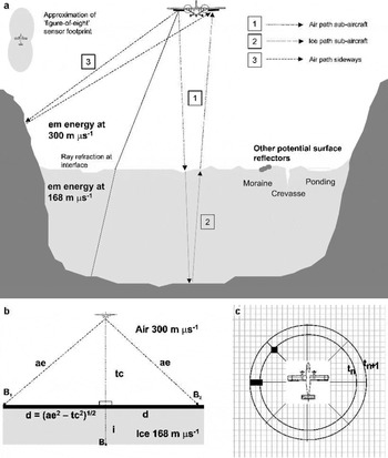
The typically broad spread of energy from an RES system means that off-nadir returns are likely. Estimates of system energy spread of ∼120° along track and ∼90° across track are fairly typical (e.g. Reference Robin, Swithinbank and SmithRobin and others, 1970) (Fig. 1). Use of a relatively high-frequency system together with a more directional antenna (e.g. phased array) would reduce such off-nadir returns, but the higher-frequency energy (hundreds of MHz) is subject to greater absorption within the ice. Reduction of flying height would produce a more focused footprint, but this option is limited by the need to maintain separation of the direct wave from the ice-surface reflection. Thus, it is probable that some part of the RES record will suffer contamination by off-nadir returns, requiring their identification by the analyst.
Various techniques can be used to separate bed returns from other returns:
Form of echo patterns. When considering the source of hyperbolic echo patterns, longer, strong tails may indicate terrain returns. However, within valleys, echo patterns may be broken or confused as energy is received from several quasi-point sources on side-walls. Assuming a footprint narrower in the cross-track direction than along-track (Fig. 1), hyperbolae from side-wall reflectors may have shorter tails due to more rapid onset within the sensor field of view.
Strength of returns. Analysis of power reflection coefficients (PRCs) can sometimes assist in discriminating between solely air-path reflections and reflections further attenuated by travel through ice. This is complicated, however, by the overlapping ranges of PRCs encountered for different interface types (Reference BamberBamber, 1987), the dependency on ice and reflector properties, and by the drop-off in the amount of power transmitted away from the sub-aircraft point.
Migration of returns. The process of migration attempts to assign returns from consecutive receiver locations to the true positions of contributing reflectors (Reference HarrisonHarrison, 1970; Reference Welch, Pfeffer, Harper and HumphreyWelch and others, 1998). However, unless it were possible to fly a sufficiently dense grid of intersecting flight-lines, there is generally only enough information available to migrate along track. Ambiguity remains, therefore, concerning the locations of returns coming from other than the sub-aircraft track.
Horizon return continuity. Looking at the general trend of a bedrock horizon across the Z-scope imparts more information than looking at single locations. There is a danger, however, of missing rises or dips in the bed, if one assumes continuity of the more clearly observable bed horizon.
Given the uncertainties discussed above, we sought to identify other sources of information which would assist in resolving ambiguity in the origin of returned power.
Use of High-Resolution Satellite Imagery to Identify Terrain Side Returns
High-resolution and accurately geo-located satellite imagery (e.g. Landsat-7 Enhanced Thematic Mapper Plus (ETM+) 15 m panchromatic (Reference Bindschadler, Dowdeswell, Hall and WintherBindschadler and others, 2001); Advanced Spaceborne Thermal Emission and Reflection Radiometer visible/near-infrared (ASTER VNIR) band 15 m resolution (Reference Yamaguchi, Kahle, Tsu, Kawakami and PnielYamaguchi and others, 1998)) or aerial photography in digital format, together with use of a differential global positioning system (GPS), allows visual inspection of the subaerial terrain overflown during RES surveys. We utilize this information on the spatial distribution of sub-aerial terrain in the interpretation of RES records. Our method is to provide information to the analyst derived from both plan-view imagery and long-profile RES data which is visualized in the same coordinate system on screen, through:
depiction of the tracked bedrock interface on satellite plan-view imagery as if due to surface reflections received from the side (termed “air-path-equivalent”);
simulation of Z-scope displays using the predicted time of returns from subaerial terrain observed in plan-view imagery (termed “echo prediction”).
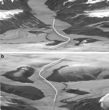
We use as an example an RES record obtained in April 2000 from part of Stygge Glacier, which is an outlet glacier of the Prince of Wales Ice Cap on Ellesmere Island, Nunavut, Canada. The track sounded lies between 78°46′57″ N, 78°13′12″ W and 78°36′41″ N, 78°46′31″ W. Within this area, the glacier rises from sea level to ∼1200 m at a slope angle of ∼4°. The upper part of the flight-line is constrained between rockoutcrops ∼2 km apart withthe rock heightaboveglacier ranging between ∼50 and ∼350 m with slopes mostly in the range ∼17° to ∼30°, and a smaller number (∼10%) of up to ∼50° (Fig. 2). These values are estimated from 500 ft (154.4 m) contours on a 1:250 000 scale topographic map and from a DEM Slope image supplied by L. Copland (University of Alberta, Canada).
Oblique views looking down-glacier (a) and up-glacier (b), illustrating the topography of the example area relevant to Figures 3 and 4, and described within the text. The flight track is marked to allow comparison with other figures and to illustrate the relationship of the topography with the aircraft position. Solid white line records aircraft location; solid grey line marks sub-aircraft track. Figure derived by L. Copland from Landsat ETM+ image and Canadian digital elevation data.
Air-path-equivalent marking of interface tracking
For our air-path-equivalent method, simple trigonometry is used based upon the aircraft terrain clearance. A plane normal to the line between the aircraft and sub-aircraft point is assumed, along with a first direct side return from a reflector on this plane in the cross-track direction (Fig.1b).
The tracked ice-surface and subglacial-bedrock interfaces are used to measure distances from the aircraft using a standard value for the speed of electromagnetic energy in air (300 m μs−1). These distances give, respectively, terrain clearance and direct air path to a hypothetical valley-side reflector on either side of the aircraft. From the terrain clearance and direct air path, it is a simple matter to calculate across-track (normal) distance from the sub-aircraft point and to plot appropriate locations at this distance left and right of the sub-aircraft point on a satellite image. This is repeated for each waveform in the along-track direction.
Interface tracking also allows the user to mark interactively features on the Z-scope display which are suspected to originate from side-wall topography. These tracks can then be viewed on satellite imagery on screen using the air-path-equivalent method.
An example of the use of the air-path-equivalent utility is shown in Figure 3. A raw intensity-modulated RES Z-scope display is shown in Figure 3a, with the corresponding flight track indicated on a Landsat image in Figure 3b. The Z-scope display is overlain by interface-tracking markers for the ice surface, bedrock and side-wall terrain. The satellite image is overlain with air-path-equivalent markers corresponding to the bedrock and side-wall terrain tracked from the Z-display. Note that, whilst one of each pair of (left-/righthand side (L/RHS)) markers may be erroneous, many of the remaining side-wall markers are coincident with or near to subaerial terrain features visible on the satellite imagery. Note, furthermore, that some of these terrain features are side-wall rock (marked “r” in Fig. 3), but others relate to medial moraines (“m”), and may also include foliation and associated ice structures linked, for example, to the location where two tributary glaciers have merged (marked “F” in Fig. 3). As the flight proceeds up towards the head of the glacier (left to right in Fig. 3), the ice is constrained within a narrowing valley with side-walls prominent on both sides (Figs 2 and 3). Here, the side-wall marker clearly demonstrates the potential for mistaking side-wall returns for subglacial bedrock returns, as illustrated in the Z-scope display in Figure 3a. This is particularly illustrated by the rock to the RHS of the flight track, which juts out towards the flight track at the entrance to this narrower valley (“r” between “1”and “2” in Fig. 3b).
(a) Raw RES Z-scope display overlain with interface track markers (ice surface and later returns). (b) Landsat ETM+ image of part of Stygge Glacier, overlain with flight-track (dashed line) and air-path-equivalent markers. The Z-scope record shown corresponds to the section of flight between “1”and “2” on the satellite image. Lettering marking coincidence of surface features with air-path-equivalent markers is as follows: m = moraine; r = rock; F = ice-structural foliation. See text for further explanation.
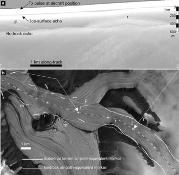
Our calculations take a simple approach using plan-view imagery to represent subaerial terrain. A full three-dimensional analysis of reflectors would require the use of a DEM and sophisticated ray tracing. At a flight terrain clearance of 400 m, a 5° surface slope in the cross-track direction would yield an error in our cross-track distance calculation of ∼32 m at a viewing angle off-nadir of 45° (i.e. approximately 2 pixels in the Landsat image. This is generally close enough to signal possible coincidence with image features). Our simpler geometry is not expected to always yield exact matches of bed track with side-wall topography, but has nonetheless been very successful in visualizing the problem from general patterns of coincidence and in providing a first-order comparison between tracked interfaces in RES records and subaerial terrain derived from satellite imagery.
Echo prediction
The echo-prediction method operates in a complementary fashion to the air-path-equivalent approach described above, again using simple trigonometry and assumptions. Plan-view imagery is used to identify subaerial terrain features, which could give rise to radar returns. The locations of these terrain features with respect to the three-dimensional along-track aircraft positions are used to predict direct air paths to and from the features and, hence, to calculate the times of receipt of reflected power. The counts of estimated reflection “hits” at each sample time are used to modulate Z-scope output intensity (Fig. 1c).
Subaerial terrain “reflectors” are identified from the digital satellite imagery by means of online adjustable thresholding of image pixel data. Exposed rock or water is typically far darker than surrounding snow or ice areas, and threshold adjustment can be made after examination of image pixel values in the area of interest (in particular where shadowing is evident or the general brightness level is lower). Examination of conventional and predicted Z-scope displays together provides the user with information on the origin of some observed reflections. The predicted Z-scope will not match the actual RES data perfectly, but the general patterns and proximity of predicted vs actual reflections is a clear aid to interpretation.
This method has the advantage over the air-path-equivalent method in accounting for potential reflectors all around the aircraft (rather than only to the sides), although it tends to predict more reflection patterns than are actually observed (having no knowledge of slope orientation). It may miss some features displaying pixel values above threshold (dependent on threshold value). For example, the feature “F” in Figure 3a has not recorded a simulated echo pattern in Figure 4b. This illustrates the need for the two complementary methods, and for care in threshold selection.
(a) Landsat ETM+ image overlain with flight track and mask of locations designated as possible terrain reflectors: white with grey dots from LHS of aircraft, black from RHS. (b) Z-scope display of echo patterns predicted from these designated reflector locations: area overlaid with black indicates returns from the RHS; area overlaid with dot pattern indicates where returns from LHS merge with those from RHS. Tx is transmitter pulse. (c) Differentiated Z-scope display showing the most prominent echo patterns. Comparison of the predicted and actual echo patterns shows a good match in general form. The left side of the Z-displays confirms that the tracking of a bedrock horizon is unlikely to be affected by the most obvious sources of subaerial terrain returns. The close agreement to the right between actual and predicted returns (marked “⋆”) indicates that it is probably correct to reject the upper candidate as a bedrock horizon, suggesting it is likely to be a side-wall return.
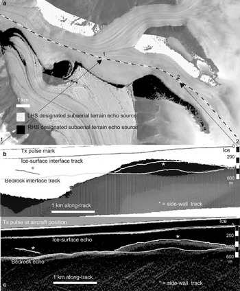
An example of the use of the echo-prediction utility is shown in Figure 4, using the same section of RES record as for the air-path-equivalent utility illustrated in Figure 3. A satellite image of the survey flight area is overlain by a mask indicating image locations designated as subaerial terrain reflectors by the echo-prediction utility (Fig. 4a). Reflectors to the RHS of the aircraft (with respect to flight direction) are masked by black and those to the LHS by white with grey dots. Marking the image pixels chosen as potential reflectors shows the user which topography is contributing to the Z-scope prediction, and aids selection of the thresholding parameter used to classify terrain in the satellite image dataset.
The Z-scope prediction display produced using these reflector sources, for the same section of flight as before, is shown in Figure 4b. The predicted Z-scope display is overlain by interface-tracking markers. Figure 4c shows the differentiated Z-scope display, so that the match in general echo patterns can be observed. Comparison reveals that the dark rise, predicted from subaerial terrain encroaching from the right side of the flight track, coincides with the actual observed echo patterns, which one might otherwise have identified as bedrock interface. The onset of this rise can be seen, as the flight approaches the narrower valley section. By contrast, the first part of the Z-scope prediction display shows the tracked bedrock interface as running clear of the most likely sources of terrain reflections. The lighter shading (from predicted LHS returns) dips downward towards the right of the record, below the prominent rise in the bedrock interface (Fig. 4b). This offers some further evidence in support of the chosen interface location above it.
The availability of a high-resolution DEM of the study area would allow a more accurate and detailed model (i.e. taking account of actual terrain elevations as well as slope and aspect to modulate the expected returned power strength). Experiments were conducted for another glacier, using a DEM constructed from contours, but it was considered that the improvement gained in positional accuracy did not warrant, for our purposes, the extra effort or cost involved in supplying an adequate DEM or additional processing time over simple trigonometric assumptions and image thresholding.
Thus, for the given example, the two techniques have complemented each other to provide useful information about sources of echo patterns. Both have signalled that the higher echo pattern (“r” in Fig. 3a), plausible as bedrock given the step-up in ice surface, is more likely to be due to surface side-returns. The air-path-equivalent markers have picked out coincidence of returns (some omitted by echo prediction) with surface features, and have lent confidence to the continuity of the bedrock delineation. The echo-prediction patterns have also provided support to delineation of a more modest bedrock high consistent with the ice-surface rise.
Conclusions
We have outlined a simple visualization technique, which assists in resolving ambiguities in the interpretation of radioecho returns, and whether these returns represent the subglacial bedrock or subaerial valley walls (Fig. 1). The method utilizes high-resolution and accurately geo-located satellite imagery to describe the spatial distribution of subaerial terrain. It provides information to an analyst on plan-view terrain and long-profile RES data which are visualized in the same coordinate system on screen (Figs 3 and 4), assisting interpretation of radio-echo origins. The technique achieves a sufficiently close matching of spatial patterns without the need for a DEM or more complicated assumptions, rendering it straightforward to implement. Finally, some complex patterns of bedrock and subaerial side-wall returns may be impossible to separate. Nonetheless, we suggest that the visualization techniques presented here are a useful aid for separation of return sources under many circumstances.
Acknowledgements
This work was carried out under U.K. Natural Environment Research Council (NERC) grant NER/A/S/1998/00015 to J.A.D. The NERC Centre for Polar Observation and Modelling (CPOM) provided image analysis facilities. Ortho-rectified Landsat-7 ETM+ imagery of Prince of Wales Ice Cap was provided by M. Sharp, University of Alberta. We are grateful to L. Copland for production of Figure 2. We thank L. Morris and C. Doake for commenting on drafts of this paper, and are grateful to J. Kohler and an anonymous referee for useful comments on the submitted paper. We also thank C. S. Hvidberg for her assistance and comments as Scientific Editor of the paper.



