


Anxiety about the competence of voters is a long-standing theme of behavioral political science. At its heart, this literature is a debate over a proposition aptly summarized by Lupia and McCubbins (Reference Lupia and McCubbins1998):
It is widely believed that there is a mismatch between the requirements of democracy and most people’s ability to meet these requirements. If this mismatch is too prevalent, then effective self-governance is impossible. The democratic dilemma is that the people who are called upon to make reasoned choices may not be capable of doing so. [p. 1, emphasis in original]
This multifaceted debate revolves around a series of questions about voters’ ability to perform their democratic function. Are voters sufficiently well informed?Footnote 1 Is the information voters do have sufficient to allow them to behave as if they were well informed?Footnote 2 Do voters respond to the right kinds of information?Footnote 3
We argue that this debate’s single-minded focus on voter behavior is misguided. Elections affect democratic performance through the interaction of politicians and voters.Footnote 4 As such, facts about voter behavior, whether “positive” or “negative,” on their own, are not informative about whether a democratic system performs well or poorly.
We consider a series of models that show just how important this interaction can be.Footnote 5 In our models, increased voter information sometimes improves democratic performance and sometimes makes democratic performance worse. Likewise, some forms of voter irrationality improve democratic performance and some forms of voter irrationality make democratic performance worse.
The key conceptual mistake of the voter behavior literature, we think, is that it applies an intuition about nonstrategic decision making to a situation of strategic interdependence. It is obviously true that, all else equal, rational people make better decisions when they have more information. If the incumbent’s policy choice, for example, is held equal, a voter does a better job of selecting good candidates when he observes that policy choice. Moreover, it is obviously true that, all else equal, a rational person makes better decisions than an irrational person. If all else is held equal, a rational voter uses the available information optimally, while an irrational voter makes systematic mistakes. But, in a strategic setting, all else is not held equal. Change the voters’ information or capacity for rational decision making, and politicians’ strategically chosen policies will change in response. Sometimes the change in politicians’ actions leads to worse policy outcomes for voters. Sometimes the change in politicians’ actions leads to there being less information with which to select good politicians for the future. In either case, the change in actions induces a trade-off, making it far from obvious that more voter information or more voter rationality is unequivocally better or unequivocally worse for voter welfare. Given this, any discussion of democratic performance that focuses narrowly on whether or not voters are competent is making a mistake.
OUR ARGUMENT WITH THE LITERATURE
The most prominent critique of voter competence argues that voters are too poorly informed to fulfill their electoral function (Campbell et al. Reference Campbell, Converse, Miller and Stokes1960; Delli Carpini and Keeter Reference Delli Carpini and Keeter1996; Kinder and Sears Reference Kinder and Sears1985). If voters lack basic information about the policy choices made by political leaders, then, the argument goes, elections are neither “a useful mechanism for selecting public leaders” nor “a credible check on the behavior of those leaders” (Delli Carpini and Keeter Reference Delli Carpini and Keeter1996, 50).
This critique has inspired a large literature. That literature’s strongest defense of voter competence argues that voters do not need detailed information about candidates or policies to act as if they were informed (Downs Reference Downs1957). An early salvo of this defense argued that voters could make good decisions based solely on retrospective evaluations of their welfare (Fiorina Reference Fiorina1981; Key Reference Key1966). Subsequent work argued that voters can use a variety of cues—party labels, statements by opinion leaders, personal economic fortunes, etc.—to fulfill their democratic function, without needing detailed information or political sophistication (Fair Reference Fair1978; Lupia Reference Lupia1994; Popkin Reference Popkin1991; Sniderman, Brody and Tetlock Reference Sniderman, Brody and Tetlock1993).
Critics of this defense argue that these informational shortcuts do not fully offset the lack of information (Bartels Reference Bartels1996), may be systematically misused (Huber, Hill and Lenz Reference Huber, Hill and Lenz2012), and can even lead to worse decision making (Lau and Redlawsk Reference Lau and Redlawsk2001). Kuklinski and Hurley (Reference Kuklinski and Hurley1994, 731) exemplify this strand of the literature when they interpret their experimental results as showing that “[a]lthough rational, and probably inevitable given the nature of large political systems, this mechanism may not be as effective as has been suggested.”
A literature further interrogating this critique explores whether voters use information rationally. One set of findings claims that voters punish incumbents for events outside the control of policy-makers (Achen and Bartels Reference Achen and Bartels2004; Healy, Malhotra and Mo Reference Healy, Malhotra and Mo2010; Leigh Reference Leigh2009; Wolfers Reference Wolfers2009). The implication drawn is that voters do not even “clear the relatively low standard of rationality implied by the ability to exclude entirely irrelevant events from the decision-making process” (Healy, Malhotra and Mo Reference Healy, Malhotra and Mo2010, 12804). Yet another set of findings claims that voters do a better job of identifying and responding to relevant information (Bechtel and Hainmueller Reference Bechtel and Hainmueller2011; Chen Reference Chen2013; Healy and Malhotra Reference Healy and Malhotra2010). Reflecting on this strand of the literature, Healy and Malhotra (Reference Healy and Malhotra2013, 285) conclude:
[T]he field is heading toward a middle ground in which voters resemble decision makers in many other domains. In many cases, a coherent logic governs voters’ choices. In other instances, voters make mistakes, often in predictable ways subject to well-known psychological biases.
From our perspective, this entire debate, for all its important disagreements, is united by a shared mistake: attempting to normatively assess democratic performance by focusing on the characteristics of only one set of relevant actors, the voters. Elections are a strategic interaction between politicians and voters. If one wants to learn about how some characteristic of voters—say, lack of information or irrationality—affects democratic performance, one must know how it affects this interaction. In the context of two canonical models of electoral accountability, we show that it is often the case that democratic performance—as measured by voter welfare—is better when voters are imperfectly informed or imperfectly rational.Footnote 6
It may seem counterintuitive—especially in light of the behavioral tradition—that poor voter information or voter irrationality could improve democratic performance. But the traditional intuition is incomplete; it ignores how changes in voter behavior affect the behavior of politicians. Indeed, in each of our models, voter welfare would be higher with better informed or more rational voters if politician behavior were held fixed. But politician behavior is not fixed—it adjusts to reflect the politicians’ anticipation of, and best response to, voter behavior.
To see how this works, think about the case of voter information. Suppose voters are poorly informed—they don’t know what policy a politician implements, and so vote based only on their overall welfare. A politician who doesn’t share the voters’ preferences must balance the desire to implement her preferred policies and the desire to improve her reelection prospects by choosing policies that lead to higher voter welfare. Consequently, faced with ill-informed voters, politicians who do not share the voters’ preferences choose a middle ground, implementing a policy between the voters’ most preferred policy and their own. Now imagine that voters become well informed—actually observing the implemented policy—but politicians continue to behave as just described. The voters are clearly better off. Their immediate payoff from policy is unchanged. But, because they can observe the actual policy choices of different politicians, they do a better job of distinguishing politicians who really agree with them on policy from those who will make future policy in service of preferences the voters do not share.
However, this unambiguous benefit is not the effect of improved voter information in equilibrium in our models. Politicians will adjust their behavior in light of the new voting strategies that increased voter information makes possible. When the voters know the actual policy that was implemented, an extreme politician faces a very stark choice. If she wants to be reelected, she must fully imitate a moderate politician, implementing a policy far from her ideal point. Alternatively, she can forego reelection and reveal herself to be extreme, at which point she may as well implement her own ideal point. Hence, when reelection incentives are large, increased voter information leads to stronger incentives for moderation by extremists. And when reelection incentives are weak, increased voter information leads to weaker incentives for moderation by extremists.Footnote 7
The argument above already suggests one complication when thinking about the value of voter information—whether it increases or decreases moderation depends on the strength of electoral incentives. But there is still one more step for a complete analysis of the effects of voter information on voter welfare. It might seem intuitive that increased incentives for moderation always benefit the voters. But this intuition is incomplete. When the extreme incumbent moderates, the voters benefit from better policy in the short run. However, such moderation also makes it harder for the voters to distinguish between extremists and moderates. Hence, when extremists moderate, the likelihood of selecting a moderate candidate for the future goes down, hurting the voters in the long run. This implies that whether voters are better off with more or less moderation depends on the relative weighting of the present and the future. And as we’ve already argued, whether informed or uninformed voters give rise to more moderation depends on the strength of electoral incentives.
Given all of this, it is entirely possible that, accounting for the strategic adjustment of politicians, overall democratic performance is actually better when voters are less well informed. The ideas that underly this result could not possibly be captured by an analysis focused solely on voter characteristics, ignoring how those characteristics affect the behavior of politicians.
A similar analysis applies to voter rationality. Quite generally, rational voters vote in a forward looking way that selects good types, not in a backward looking way that maximizes incentives (Fearon Reference Fearon, Przeworski, Stokes and Manin1999). That is, a rational voter votes retrospectively—i.e., based on past outcomes—only because those outcomes are informative about expected future outcomes. As Fearon shows, this is true as long as the past provides even a tiny amount of information about the future. The upshot of this observation is that there is every reason to expect rational reelection decisions to differ from those that would maximize voter welfare from the ex ante point of view.
To see this, consider again the incentives of an extreme politician facing uninformed voters. Changing the voters’ behavior away from the rational reelection rule, and holding the incumbent’s policy choice fixed, reduces the voters’ ability to select the best candidate for the future. But, as before, a full analysis requires taking account of the change in politician behavior that the shift to an irrational reelection rule induces. If this shift leads to more moderate policy, then the voters benefit from better immediate policy, but have a harder time selecting the right politician for the future. If this shift leads to more extreme policy, then the voters suffer in terms of immediate policy but have more information with which to select the right politician for the future. As before, whether moderation helps or harms voter welfare overall depends on how the present and future are weighted. The important point is that the voters would be better off if they could somehow commit to vote in a way that balanced the benefits of selection against the benefits of affecting moderation. The sequential structure of the interaction makes such a commitment incredible for rational voters, opening up the possibility that irrationality could improve voter welfare. Indeed, as we show, the typical case is that at least some amount of irrationality makes voters better off.
We want to emphasize what we are not arguing. Our results do not say that democratic performance would clearly be better were voters less informed or less rational, relative to the status quo. Nor do they say that democratic performance would clearly be worse were voters less informed or less rational, relative to the status quo. Rather, our point is that any particular collection of empirical facts about voter characteristics—be it evidence of voter incompetence or voter competence—has, on its own, no particular implication for democratic performance one way or the other. As such, the empirical debates over voter information and voter rationality, while informative about voter characteristics, do not speak in any straightforward way to the fundamental normative concerns that seem to motivate them.
MODELING ACCOUNTABILITY
Any situation of electoral accountability involves several actors, including politicians and voters. Our approach will focus on models with three players: an incumbent, a challenger, and a representative voter.Footnote 8
The incumbent politician has to take some action in order to govern. The incumbent politician’s actions can range from choosing ideological positions to exerting costly time, effort, or political capital to procure public goods, to choosing whether or not to engage in corruption. In each case, some actions by the incumbent are better for voters than others. To make the situation interesting, we typically think there is not perfect alignment of preferences over actions between the incumbent and the voter.
The voter makes some observations and decides whether to reelect the incumbent or replace her with the challenger. A voter’s observations can range from very sparse information about his personal welfare, to detailed knowledge about the actions and/or preferences of the politicians.
Our points about voter information and voter rationality are quite general. They do not depend on the particulars of the kind of actions politicians take or the kind of observations the voter makes. To demonstrate this, we will develop each of our points in two models. These models, while both canonical, differ significantly in terms of what actions are possible and what voter observation of incumbent choice can reveal.
Our first model is one of ideological policy choice. Politicians choose policies in a one-dimensional policy space, and differ from voters and from each other in terms of policy preferences. Our second model is one of costly effort to enhance performance on a valence dimension. Politicians choose how much effort to exert (this can be interpreted either as work on providing public goods or foregoing opportunities for corruption). Politicians differ from voters in that effort has private costs to the politicians, while politicians differ from one another in terms of how competent they are at governance.
Some settings of electoral accountability are best thought of in terms of politician ideology and policy choice, as captured in our first model. Others are best thought of as situations where all voters agree that they want competent management, as captured in our second model. All of our results hold for both the policy and effort choice models. While we focus on the policy choice model in the main text, analogous results for the effort choice model are presented in Appendix B.
Ideological Policy Choice Model
There are a voter, an incumbent politician (I), and a challenger (C). There are two periods. In each period, t, the politician in office chooses a policy,
 $a_t \in \mathbb {R}$
. The voter’s ideal policy is zero.
Each politician is of one of two types, moderate or extremist. We assume that a moderate politician chooses a policy equal to the voter’s ideal point whenever she is in office. An extremist politician has her own ideal point and chooses policy strategically.
Both the voter and the extremist politicians have quadratic-loss payoffs. We assume the incumbent is from the right-wing party, while the challenger is from the left-wing party. Hence, the incumbent is either a moderate or has an ideal point equal to θ > 0. The challenger is either a moderate or has an ideal point equal to − θ. The types of the politicians are determined independently, and the probability that a politician is the moderate type is p ∈ (0, 1).
The voter’s payoff in period t is an additive function of his policy payoff and unobservable noise (ε t ). That is, the voter’s payoff in period t, if the policy choice is at , is
 \begin{equation*}
- a_t^2 + \epsilon _t.
\end{equation*}
Each ε is drawn independently from a normal distribution with mean 0 and variance 1.
Extreme politicians have purely ideological preferences. In period t, an extremist politician with ideal point θ gets a payoff from policy at of
 \begin{equation*}
-(\theta - a_t)^2.
\end{equation*}
Extreme politicians receive ideological payoffs each period, regardless of whether or not they are in office. (Recall that moderate politicians are behavioral types who always choose the voter’s ideal point, so we do not need to specify their payoffs.)
Players have payoffs given by a weighted average of first period and second period payoffs. The weight on the second period is δ, with 0 < δ < 1. The weight on the first period is (1 − δ).
All random variables are independent. The voter does not directly observe the politicians’ types. The voter always observes his payoff. We will consider situations in which the voter does not observe the policy choices (uninformed voters) or does observe the policy choices (informed voters).
The timeline of the game is as follows:
-
1. Nature draws all random variables.
-
2. The incumbent chooses a policy a 1.
-
3. The voter observes his payoff and (possibly) the policy and then chooses whether to elect the incumbent or the challenger.
-
4. The winner of the election chooses policy a 2.
-
5. Payoffs and (possibly) policy are observed and the game ends.
Throughout we assume that the voter, if he is indifferent, votes for the incumbent.
Effort Choice Model
There are a voter, an incumbent politician (I), and a challenger (C). There are two periods. Each politician, j, is characterized by an ability (θ
j
). In each period t, the politician in office chooses a level of effort
 $a_t \in \mathbb {R}_+$
.
The outcome in a period t is a function of three factors: the competence of the politician in office (θ t ), the effort of the politician in office (at ), and unobservable noise (ε t ). The outcome in period t is
 \begin{equation*}
\pi _t = f(a_t,\theta _t) + \epsilon _t.
\end{equation*}
Each ε is drawn independently from a normal distribution with mean 0 and variance 1.
Effort and competence both increase the expected outcome. In particular, f is strictly increasing in a and θ and is continuously differentiable in a.
Politician j’s ability (θ
j
) is drawn from
 $\lbrace \overline{\theta }, \underline{\theta }\rbrace$
, where
 $\overline{\theta }>\underline{\theta }$
. The probability a politician is the high ability type is p ∈ (0, 1). All random variables are independent.
No player observes the θ’s or the ε’s. We will consider situations in which the voter does not observe the action of the politician in office (uninformed voters) or does observe the action (informed voters).
The voter’s payoff is the weighted average of the two outcomes,
 \begin{equation*}
(1-\delta )\pi _1 + \delta \pi _2,
\end{equation*}
with 0 < δ < 1. Each politician gains a benefit of 1 for being in office and suffers a cost of effort given by the increasing, strictly convex, and differentiable cost function c( · ).
The timeline of the game is as follows:
-
1. Nature draws all random variables.
-
2. The incumbent chooses effort a 1.
-
3. The voter observes the outcome π1 and (possibly) the action and then chooses whether to elect the incumbent or the challenger.
-
4. The winner of the election chooses effort a 2.
-
5. The voter observes the outcome π2 and (possibly) the action and the game ends.
VOTER INFORMATION
The policy choice game comes in two versions. In the first version, the voter is informed, in the sense of actually knowing the policy implemented by the politician. This idea of an informed electorate corresponds to that implicit in the behavioral literature which, for example, asks whether voters are aware of votes taken by their representatives. In the second version, the voter is uninformed about policy, knowing only his own welfare. This corresponds to rational retrospection in the spirit of Fiorina (Reference Fiorina1981). In either case, the politicians know whether or not the voter is informed.
Our uninformed voter is able to extract some useful information from the cue provided by his welfare. But, consistent with the empirical results of Bartels (Reference Bartels1996) and others, this information is not enough to allow him to vote as if he were fully informed. Our central point is that this gap between informed and uninformed voting can very well make the voter better off in equilibrium. That is, we show that it is entirely possible that, even when information is free, voters are better off when uninformed.Footnote 9
The voter’s motivation is the same in each version. His payoff is a sum of payoffs from each of the two periods. However, the voter chooses whether or not to reelect the incumbent after his first period payoffs are already determined. Hence, at election time, the rational voter simply acts to maximize his second period payoff. (This is just as in Fearon (Reference Fearon, Przeworski, Stokes and Manin1999).) In the second period, the politician in office is unconstrained by a future election. Hence, in the second period, the policy will be the voter’s ideal point if the politician in office is a moderate or the politician’s ideal point if the politician in office is an extremist. Given this, the voter wants to elect the politician most likely to be moderate.
This means that if the incumbent is an extremist, she faces a trade-off. She can increase her probability of reelection by taking an action that lowers her first period welfare—in particular, choosing a more moderate policy. She must balance the benefits of reelection against these costs. As we will see below, the exact nature of this trade-off depends critically on whether or not the voter is informed about the actual policy choice.
Informed Voter
Suppose the voter is informed. What will an extremist do in the first period? For any policy choice other than the voter’s ideal point, the extremist reveals her type, guaranteeing that she will be replaced.Footnote 10 Knowing she can’t get reelected without completely sacrificing today’s policy, the extremist will either moderate completely (choosing the voter’s ideal policy) or not at all (choosing her own ideal policy). Which she chooses is determined by how strongly she is motivated by reelection concerns—i.e., how much she cares about the future and how bad she thinks her replacement is likely to be if she is not reelected.
Let’s see this in the model. The extremist’s payoff from choosing her own ideal point and foregoing reelection is
 \begin{equation*}
(1-\delta )\times 0 - \delta \left[p \theta ^2 +(1-p) 4 \theta ^2\right].
\end{equation*}
The first term represents her first period payoff from choosing her ideal policy. The second term represents her discounted second period payoff, given that with probability p the replacement is a moderate and chooses policy 0 and with probability 1 − p the replacement is an extremist from the other party and chooses policy − θ. Her payoff from choosing the voter’s ideal point and achieving reelection is
 \begin{equation*}
-(1-\delta )\theta ^2 + \delta \times 0.
\end{equation*}
Again, the first term represents her first period payoff from choosing the voter’s ideal policy. The second term represents her second period payoff, given that, once reelected, she implements her ideal policy.
Comparing these two payoffs, the extreme incumbent prefers to choose her own ideal point if and only if
 \begin{equation*}
\delta \le \frac{1}{5 - 3p}.
\end{equation*}
This inequality makes precise our earlier assertion that the extreme incumbent’s behavior is dictated by the strength of reelection motivations. Reelection motivations are weak when the future is relatively unimportant (low δ) and when the incumbent’s replacement is unlikely to be an extremist from the other party (p large). The inequality says that, when reelection motivations are weak, the extreme incumbent chooses her own ideal point. This allows the voter to perfectly distinguish types, but at the cost of sometimes getting extreme policy in the first period. When reelection motivations are strong, the extreme incumbent chooses the voter’s ideal point. This provides the voter with good first period policy, but at the cost of being unable to distinguish types.
Given this analysis, the voter’s ex ante expected welfare when he is informed is
 \begin{equation}
\hspace*{-12pt}W^{I}(p,\delta ,\theta ) = \left\{
\begin{array}{@{}l@{}}
- \delta (1-p)\theta^{2}, \\[3pt]
\qquad {\rm if }\, \delta \ge \frac{1}{5 - 3p} \\[3pt]
- (1-p) [(1-\delta )\theta^{2} + \delta (1-p)\theta^{2}], \\[3pt]
\qquad {\rm else.} \\
\end{array}\right.
\end{equation}
Uninformed Voter
Now suppose the voter is uninformed. If the voter is not informed, he cannot perfectly identify whether the incumbent is extreme or moderate even if different types choose different policies. Instead, the voter forms beliefs about the likely type of the incumbent after observing his welfare.Footnote 11 This creates different incentives for an extreme incumbent than those that existed with an informed voter. When the voter was informed, the only way for an extreme incumbent to have any chance of reelection was to mimic a moderate politician, moving her policy choice all the way to the voter’s ideal point. But now—because the voter’s reelection rule conditions on outcomes, not actions—an extreme incumbent can achieve a small increase in probability of reelection with a small policy move in the direction of the voter’s ideal point. Unlike in the case of the informed voter—where the extreme incumbent’s behavior was either fully moderate or not moderate at all—with an uninformed voter, the extreme incumbent’s behavior will strike a balance between the benefit of a small increase in probability of reelection and the cost of small amounts of policy moderation.
To see this in the model, let’s look at equilibrium with an uninformed voter. Since the voter is uninformed, he does not know what action the incumbent took. Hence, his interpretation of the outcome will depend on his conjecture about the action an extreme incumbent would take. (He, of course, knows what action a moderate incumbent would take.) We call this conjecture
 $\tilde{a}$
. We then use this conjecture, and Bayes’ rule, to calculate the voter’s posterior beliefs about the likelihood that the incumbent is moderate, given a payoff of π and a conjecture
 $\tilde{a}$
:
 \begin{equation*}
\frac{p \phi (\pi )}{p\phi (\pi ) + (1-p)\phi (\pi + \tilde{a}^2)},
\end{equation*}
where ϕ is the standard normal probability density function. The voter reelects if that posterior is greater than or equal to the probability that the challenger is moderate (p), which means the voter reelects if and only if:
 \begin{equation*}
\frac{\phi (\pi )}{\phi (\pi + \tilde{a}^2)} \ge 1.
\end{equation*}
The left-hand side is increasing in π (this is because the normal distribution satisfies the monotone likelihood ratio property). This implies that the voter uses a simple cutoff rule—he reelects the incumbent if his payoff is at least as large as
 $\overline{\pi }(\tilde{a})$
. This cutoff rule satisfies
 \begin{equation*}
\frac{\phi (\overline{\pi })}{\phi (\overline{\pi } + \tilde{a}^2)} = 1.
\end{equation*}
Solving, we have
 \begin{equation}
\overline{\pi }(\tilde{a}) = - \frac{\tilde{a}^2}{2}.
\end{equation}
 $\overline{\pi }$
. The extreme incumbent believes that if she takes action a she is reelected if
 \begin{equation*}
-a^2 + \epsilon _1 \ge \overline{\pi }.
\end{equation*}
Hence, as illustrated in Figure 1, her probability of reelection is
 \begin{equation*}
1- \Phi \left(\overline{\pi } + a^2\right).
\end{equation*}
The closer the extreme incumbent’s policy choice is to zero (the voter’s ideal policy), the more likely she is to be reelected.
FIGURE 1.

If reelected, the extreme incumbent implements her ideal policy tomorrow, getting a payoff of zero. If she is not reelected, then the challenger holds office in the second period. With probability p the challenger is a moderate who implements the voter’s ideal point, giving the first period extreme incumbent a payoff of − θ2. With probability 1 − p the challenger is an extremist from the other party who implements a policy that gives the first period extreme incumbent a payoff of − 4θ2. Given this, if an extreme incumbent conjectures that the voter uses the reelection rule
 $\overline{\pi }$
, then her best response is to choose a policy that solves the following:
 \begin{eqnarray*}
\max _{a}\hspace*{-1pt} -\hspace*{-1pt}(1\hspace*{-1pt}-\hspace*{-1pt}\delta )(\theta - a)^2 - \delta \Phi \left(\overline{\pi } + a^2\right)\left[p \theta ^2 +(1\hspace*{-1pt}-\hspace*{-1pt}p) 4 \theta ^2\right].
\end{eqnarray*}
Before solving for the extreme incumbent’s optimal policy choice, given that the voter uses a cutoff rule, it is important to see that there are two groups of policies the extreme incumbent will never consider—policies less than zero or greater than θ. The extreme incumbent’s first period welfare is single peaked and maximized at a 1 = θ and her probability of reelection is single peaked and maximized at a 1 = 0. Hence, she will not choose a policy to the left of zero because doing so gives her a lower probability of reelection and a lower first period payoff than does choosing zero. Similarly, she will not choose a policy to the right of θ because doing so gives her a lower probability of reelection and a lower first period payoff than does choosing θ. We record these facts in the following result.
Lemma 1 Given that the incumbent believes that the voter uses a cutoff rule, it is never a best response to choose a > θ or a < 0.
Proof. Follows from the argument in the text. ▪
We can now solve for the extreme incumbent’s best response. Taking first-order conditions, we have that the extremist’s best response,
 $a_*(\overline{\pi })$
, must satisfy
 \begin{eqnarray}
\eqcellsep\eqcellsep 2(1-\delta )[\theta - a_*(\overline{\pi })]\nonumber\\
\eqcellsep\eqcellsep \quad - 2 a_*(\overline{\pi }) \delta \phi \left(\overline{\pi } + a_*(\overline{\pi })^2\right)\left[p \theta ^2 +(1-p) 4 \theta ^2\right] =0.\nonumber\\
\end{eqnarray}
The intuition for this first-order condition is as follows. The marginal cost of a small amount of policy moderation away from the voter’s expectation results from a worse policy for the incumbent in the first period. (The first term in Equation (3).) The marginal benefit of a small amount of policy moderation away from the voter’s expectation comes from an increase in the probability of reelection, resulting in a better expected policy payoff in the second period. (The second term in Equation (3).) As shown in Figure 2, this marginal benefit is proportional to the height of the density of the distribution of the shock ε1 at the voter’s cutoff rule.
FIGURE 2.

An equilibrium of this game is characterized by both players playing best responses to their conjectures about the other player, and both players’ conjectures being correct. Hence, we can find the equilibrium choice by the extremist, a
*, by substituting
 $\overline{\pi }(a_*) = -\frac{a_*^2}{2}$
into the first-order condition:
 \begin{eqnarray}
(1\hspace*{-1pt}-\hspace*{-1pt}\delta )(\theta \hspace*{-1pt}-\hspace*{-1pt} a_*) \hspace*{-1pt}-\hspace*{-1pt} a_*\delta \phi \left( \frac{{a}_*^2}{2}\right)\left[p \theta ^2 \hspace*{-1pt}+\hspace*{-1pt}(1-p) 4 \theta ^2\right] \hspace*{-.5pt}=\hspace*{-.5pt} 0.\nonumber\\
\end{eqnarray}
We have shown that, if there is a pure strategy equilibrium to the game, the action taken by an extreme incumbent solves Equation (4). There is one loose end in this analysis—a pure strategy equilibrium might not exist. A sufficient (though not necessary) condition for a pure strategy equilibrium to exist is for the incumbent’s objective function to be concave. The next result gives conditions under which this is the case. We assume that these conditions hold throughout the main body of the article. (Appendix C uses computation to study examples in which the conditions below do not hold.)
Proposition 1
In any pure strategy equilibrium, the extreme incumbent action a
*
is given by the solution to Equation (4). A pure strategy equilibrium exists if either
 $\theta \le \left(\frac{1}{2}\right)^{1/4}$
or
 \begin{equation*}
\delta \le \frac{\sqrt{2\pi }}{\sqrt{2\pi }+[p+(1-p)4]\theta ^2(2\theta ^4-1)}.
\end{equation*}
(Omitted proofs are in Appendix A.)
It is straightforward from the equilibrium condition in Equation (4) that the equilibrium choice of policy by the extremist is neither the voter’s ideal policy (
 $a_* \not= 0$
), nor her own ideal policy (
 $a_* \not= \theta$
). Rather, it is strictly in between.
The voter’s ex ante expected welfare if he is uninformed is
 \begin{eqnarray}
\eqcellsep\eqcellsep W^{U}(p,\delta ,\theta ) = - p\delta \Phi \left(\frac{-a_*^2}{2}\right)(1-p)\theta ^2 - (1-p)\nonumber\\
\eqcellsep\eqcellsep\quad\times\,\left((1-\delta )a_*^2 + \delta \left( \left[1- \Phi \left(\frac{a_*^2}{2}\right)\right]\theta ^2\right.\right.\nonumber\\
\eqcellsep\eqcellsep\quad \left.\left. + \Phi \left(\frac{a_*^2}{2}\right)(1-p)\theta ^2\right) \right).
\end{eqnarray}
Voter Welfare With and Without Information
The voter’s welfare is determined by two factors: how close the first period policy is to his ideal point and how good a job he does selecting moderate types for the second period. These two factors imply an important subtlety in thinking about whether voters are better off with or without information. In particular, one might have thought that voters are obviously better off whenever the extreme incumbent chooses the voter’s ideal point in the first period. (This would, for instance, imply that voters are better off being informed when reelection incentives are strong.) That intuition is wrong. Clearly, the voter’s first period welfare is maximized in such a circumstance. But when extremists choose the voter’s ideal point, the voter is unable to distinguish extremists from moderates. As a result, the voter’s second period welfare is minimized in such a circumstance.
Now we can see that there is a trade-off, in terms of voter welfare, comparing informed and uninformed voters. When reelection motivations are strong, extreme incumbents fully moderate in the first period with informed voters but not with uninformed voters. Hence, with strong reelection motivations, first period voter welfare is higher with informed voters and second period voter welfare is higher with uninformed voters. When reelection motivations are weak, informed voters do a better job of selecting moderate types. However, informed voters use a reelection rule that fails to induce extreme politicians to moderate at all in the first period, while uninformed voters use a reelection rule that induces at least some first period policy moderation by extremists. Hence, with weak reelection motivations first period voter welfare is higher with uninformed voters and second period voter welfare is higher with informed voters.
The argument above implies that whether voter information is good or bad for democratic outcomes depends on the strength of reelection motivations and the relative voter weighting of current and future payoffs. When the future is relatively important, the voter cares more about second period payoffs than first. But when the future is important reelection motivations are also strong, which, as we’ve seen, means that informed voters get good first period payoffs but bad second period payoffs, relative to uninformed voters. When the future is relatively unimportant, the voter cares more about first period payoffs than second. But when the future is unimportant, reelection motivations are also weak, which, as we’ve seen, means that informed voters get good second period payoffs but bad first period payoffs, relative to uninformed voters. The following result shows that, because of these trade-offs, the voter is better off being uninformed for a nontrivial set of parameter values. Figure 3illustrates this fact.
FIGURE 3.

Proposition 2
There exist two open sets,
 $\mathcal {O}_S, \mathcal {O}_P \subset (0,1)^3$
such that
-
1. If
 $(p,\delta ,\theta _E) \in \mathcal {O}_S$
, then if the voter is informed the equilibrium is separating (strong reelection incentives).
-
2. If
$(p,\delta ,\theta _E) \in \mathcal {O}_P$
, then if the voter is informed the equilibrium is pooling (weak reelection incentives).
-
3. If (p, δ, θ E ) is in either, then voter welfare is higher when the voter is uninformed than when the voter is informed.


The existing literature takes it as obvious that increased voter information is good for voter welfare. Yet our models suggest this is not the case—voter information can harm voter welfare. Taking the interactive nature of elections into account via an equilibrium analysis, thus, has dramatic implications for the normative consequences of voter information.
Matters are even more straightforward in the effort choice model. As we show in the appendix, in that model, if effort and ability are weakly complementary in the production of public goods, then the voter is strictly better off not being informed. In particular, a less informed voter provides stronger incentives for effort and does at least as well at selecting good types. If effort and ability are strict substitutes, then the voter faces a trade-off—a less informed voter still provides stronger incentives, but now does a worse job of selecting good types.
VOTER RATIONALITY
The literature on voting and democratic competence did not go in the direction suggested by our analysis above, where we show that increased information can help or harm voters, once we take into account the strategic response of politicians. Instead, the debate has centered on how closely uninformed voters can approximate the behavior of informed voters. It is here that rationality has been thought particularly relevant.
Based on their study of the electoral consequences of events seemingly outside the control of incumbents, Achen and Bartels (Reference Achen and Bartels2004, 35–36) claim that
Democracy must be defended some other way, if it is to be defended at all. ...rational retrospective voting is harder than it seems, and blind retrospection sometimes produces consistently misguided patterns of electoral rewards and punishments.
A subsequent literature continues to explore whether voter responses to a host of seemingly irrelevant events are in fact evidence of irrationality or whether they are consistent with more subtle rational accounts (Ebeid and Rodden Reference Ebeid and Rodden2006; Healy and Malhotra Reference Healy and Malhotra2010; Healy, Malhotra and Mo Reference Healy, Malhotra and Mo2010; Kayser and Peress Reference Kayser and Peress2012; Leigh Reference Leigh2009).
Making normative assessments of democratic performance based on the empirical results in this literature would be another instance of the mistake we pointed to in the previous section. As with changes in voter information, whether or not voters are expected to behave rationally affects the strategic behavior of politicians. Hence, it is entirely possible for democratic performance to be better with irrational voters than with rational voters or vice versa. Indeed, as we show, rational voting almost always leads to “misguided patterns of electoral rewards and punishments,” in that there is almost always some level of voter irrationality that leads to higher voter welfare than does full rationality.
Before turning to the analysis, we need to deal with the conceptually thorny issue of what we mean by voter welfare when the voter is irrational. Here is our approach: In our models, we specify rational voter preferences. Irrationality then means that the voter’s behavior is not sequentially rational given his preferences and beliefs. We will thus always be able to refer back to the rational preferences of the voter to give a welfare analysis, even when the voter behaves irrationally.
In each of our models, the voter’s ex ante welfare depends on both the first period action and the likelihood that a good type is in office in the second period. Moreover, as we’ve seen, a rational voter in these models uses his vote to “select good types” (Fearon Reference Fearon, Przeworski, Stokes and Manin1999). This means that the voter uses a voting rule that maximizes the probability of a good type in the second period, conditional on the first period information. The voter does not use a voting rule designed to maximize his ex ante welfare. As such, there is no reason to believe that the rational voting rule—the rule that maximizes a voter’s future payoffs given his beliefs—will be the voter welfare-maximizing rule. This opens up the possibility that voters who behave irrationally might actually vote in a way that is better for voter welfare.
What is the impact, starting from an equilibrium, of a small increase in the stringency of the voter’s reelection rule away from the rational reelection rule? (By increased stringency, we mean the use of a higher welfare threshold for reelection.) Such a change has three effects on the voter’s welfare. Holding fixed the incumbent’s action, such a change directly decreases the quality of selection. This tends to harm voter welfare. In addition, there are two effects on voter welfare that come from the fact that a change in the voter’s reelection rule leads to a change in the incumbent’s action. First, a change in the incumbent’s action directly affects the voter’s first period welfare. Second, a change in the incumbent’s action may change how informative first period performance is about the incumbent’s type and, thus, may affect the quality of selection. These latter two effects can increase or decrease voter welfare, depending on how the action changes and the relative importance of first and second period welfares.
Let’s see how this works in the policy choice model with an uninformed voter. We assume that the politicians know whether or not the voter is rational.
As we saw in Equation (3), if the extreme incumbent believes the voter uses reelection rule
 $\overline{\pi }$
, then she takes action
 $a_*(\overline{\pi })$
. Hence, the voter’s welfare, as a function of the anticipated reelection rule, is
 \begin{eqnarray*}
W(\overline{\pi }) &=& -(1-\delta )(1-p)a_*(\overline{\pi })^2 - \delta {[}p \Phi (\overline{\pi })(1-p) \theta ^2\\[3pt]
&& +\,(1-p){(}( 1-\Phi (\overline{\pi } + a_*(\overline{\pi })^2)) \theta ^2 \\[3pt]
&& +\, \Phi (\overline{\pi } + a_*(\overline{\pi })^2)(1-p)\theta ^2{)} {]}.
\end{eqnarray*}
We can see the three welfare effects of a change in the anticipated reelection rule by differentiating:
 {\fontsize{8}{10}\selectfont{\begin{eqnarray*}
&&\frac{d W(\overline{\pi })}{d \overline{\pi }} = \overbrace{\delta p(1-p)\theta ^2( \phi (\overline{\pi } + a_*(\overline{\pi })^2)-\phi (\overline{\pi })) }^{\mbox{effect of $\overline{\pi }$ on selection}} \\
&&\qquad \underbrace{- \frac{d a_*(\overline{\pi })}{d\overline{\pi }}}_{\mbox{effect of $\overline{\pi }$ on $a_*$}} \\
&&\quad\times\,\left[\underbrace{2(1-\delta )(1-p)a_*(\overline{\pi })}_{\mbox{direct effect of $a_*$}} - \underbrace{\delta 2a_*(\overline{\pi })p(1-p)\theta ^2\phi (\overline{\pi } + a_*(\overline{\pi })^2)}_{\mbox{effect of $a_*$ on selection}}\right].
\end{eqnarray*}}}
Given all of these effects, how do we know that a small amount of voter irrationality can improve voter welfare? Here it is important that the equilibrium rule is chosen by the voter to select good types. This means that standard facts about optimization (i.e., the envelope theorem) imply that the direct effects of small changes away from the equilibrium voting rule on the quality of selection are second order. Hence, the only important effects of an increase in the stringency of the voter’s reelection rule are the effects that operate through the change in the incumbent’s action. As long as the effect on first period welfare and second period selection don’t exactly offset, an irrational increase in stringency thus either strictly increases or strictly decreases the voter’s welfare. If it strictly increases the voter’s welfare, we have that some level of voter irrationality improves voter welfare. If it strictly decreases the voter’s welfare, then it is straightforward to show that a small irrational decrease in stringency will increase the voter’s welfare.
It is not obvious that the two effects don’t offset, since they always pull in opposite directions. Suppose a change in the voter’s reelection rule leads an extreme incumbent to choose a more moderate policy. On the one hand, this improves the voter’s first period welfare. On the other hand, when extreme incumbents behave more like moderate incumbents, it is more difficult for the voter to distinguish between them. Hence, this same change worsens selection, harming the voter’s second period welfare. A similar argument, of course, holds for a change in the voter’s reelection rule that leads an extreme incumbent to choose a more extreme policy. Despite the fact that these two effects pull in opposite directions, the following result shows that generically they do not fully offset, so there generically exists some level of voter irrationality that enhances voter welfare.Footnote 12
Proposition 3
Almost always, there exists an irrational reelection rule that, when best responded to, yields higher voter welfare than the equilibrium welfare. That is, for any parameter vector (p, δ, θ) outside of a closed set of measure zero, there exists a
 $\overline{\pi } \not= \overline{\pi }_*(p,\delta ,\theta )$
such that
 \begin{equation*}
W(\overline{\pi }) > W{(}\overline{\pi }_*(p,\delta ,\theta ){)}.
\end{equation*}
The argument above explaining the proof of Proposition 3 is based on small deviations from rationality. However, it is important to note that we aren’t saying that only a small amount of voter irrationality is voter welfare enhancing. Larger amounts of voter irrationality can also sometimes result in better outcomes for voters. The difference between small amounts of irrationality, of the sort analyzed in Proposition 3, and large amounts of irrationality is that small amounts of irrationality only matter for welfare through their effect on the incumbent’s policy choice (which, of course, then affects both first period payoffs and the quality of selection). Once one considers a larger amount of irrationality, there is also the direct effect on selection that must be taken into account and which cuts against the benefits of irrationality. But that doesn’t mean that larger amounts of irrationality never lead to better voter welfare than does full rationality. It depends on the relative magnitudes of competing effects. The next section explores this issue in greater depth for a particular type of irrationality that is of interest in the empirical literature.
Voters Who Fail to Filter
An important part of the empirical literature purports to demonstrate a particular kind of voter irrationality—that voters hold politicians responsible for observable events (like natural disasters, economic shocks, or football losses) that the voters should know are outside of the politicians’ control. Here we show that this kind of irrationality can enhance voter welfare. Importantly, the benefits of irrationality can be shown to hold even for nonmarginal deviations from full rationality.
To see this, consider a model that is virtually identical to the policy choice model with an uninformed voter, with the exception that the voter’s welfare in period t is now a function of observable events not affected by the politician in office (ν t ) in addition to the two factors from the previous model—the policy choice of the politician (at ) and unobservable noise (ε t ). The voter’s welfare in period t, then, is
 \begin{equation*}
-a_t^2 + \nu _t + \epsilon _t.
\end{equation*}
Each ν is observable and drawn independently (of all other random variables) from a normal distribution with mean 0 and variance σ2 ν. All other random variables are as above. Payoffs are as before.
First, consider what happens with a rational voter. A rational voter filters out the observable events not affected by the politician in office and then behaves exactly as in the previous model. That is, rather than using his welfare to update his beliefs, a rational voter uses his welfare minus ν1. The equilibrium incentives for an extreme incumbent are thus exactly as before.
Next, consider what happens with an irrational voter who fails to filter the observable event, using his welfare (including ν1) to update his beliefs, but then best responds to those incorrect beliefs. The analysis of voter electoral behavior is very similar to that with rational voters. Of course, voters who fail to filter use the “wrong” cutoff rule in the sense of sometimes electing incumbents who are less likely to be moderates than the challenger or not reelecting incumbents who are more likely to be moderates than the challenger. From the extremist incumbent’s perspective, this failure to filter events that are not in the incumbent’s control is equivalent to adding noise to the voter’s decision, since the voter will vote based on events which, from the incumbent’s perspective, are random luck. As such, one can view the variance of ν1 as a measure of the amount of voter irrationality—the larger is σν, the larger in magnitude, on average, is the observable welfare shock that the voter is failing to filter.
The key result for us is that the rule used by a fail-to-filter voter provides different incentives for policy moderation by the extreme incumbent than does the rule used by a rational voter. Since the rational voter’s rule is not ex ante welfare maximizing—in particular, because welfare depends on the first period action—changing those incentives can be welfare enhancing.
Recall from Figure 2 that the marginal benefit to an extreme incumbent of moderating her policy choice comes from an increase in probability of reelection, an increase that is proportional to the height of the density of the shock at the voter’s reelection cutoff. Since a rational voter filters out the observable shock, matters are identical to the standard model if the voter is rational. But when the voter fails to filter there is the extra random component that comes from the observable events that the voter fails to filter out. So from the perspective of the incumbent, the shock has a bigger variance.
This increase in variance changes the incumbent’s marginal benefit from moderation. However, there is an important subtlety. The increase in variance can increase or decrease the extreme incumbent’s marginal benefit from moderation, depending on whether the increase in variance lowers or raises the height of the density at the voter’s reelection cutoff. This, in turn, depends on how close the reelection cutoff (
 $\overline{\pi }$
) is to the mean of the distribution of voter payoffs induced by the policy choice ( − a
2). As shown in Figure 4, when the cutoff rule is close to the expected payoff (so
 $\overline{\pi } + a^2$
is close to zero), incentives to moderate are weaker with a fail-to-filter voter than with a rational voter. When the cutoff rule is far from the expected payoff, incentives to moderate are stronger with a fail-to-filter voter than with a rational voter.
FIGURE 4.

It might seem intuitive to think that increased incentives for moderation in the first period always benefit the voter. But, as we’ve pointed out previously, this intuition is incomplete. When the extreme incumbent moderates, expected first period payoffs go up. However, moderation makes it harder for the voter to distinguish between extremists and moderates, reducing the quality of selection and, consequently, expected second period payoffs. This implies that whether voters are better off with more or less first period moderation depends on the relative weighting of the two periods. Hence, whether fail-to-filter voters yield better welfare than rational voters depends both on whether they strengthen or weaken incentives for moderation and on whether voters are better off with more or less moderation.
Given this, under what conditions is voter welfare higher with irrational, fail-to-filter voters than with rational voters? Recall, from Equation (2), that the rational voter’s equilibrium cutoff rule is the mid-point between his own ideal point and the extreme incumbent’s policy choice. Moreover, as we saw in Figure 4, incentives for moderation are stronger with a fail-to-filter voter than with a rational voter when the extreme incumbent’s policy choice is far from the voter’s cutoff rule (so that
 $\overline{\pi } + a^2$
is far from zero).
Consider, then, the combination of two circumstances. First, extreme politicians have ideal points far from the voter’s ideal point (θ large). Second, reelection concerns do not loom very large in the incentives of an extreme incumbent—i.e., the future isn’t very important (δ small) or the incumbent’s replacement, should she not be reelected, is unlikely to be an extremist of the other party (p small). In this case, the incumbent’s policy choice a * will be close to her own ideal point and far from the rational voter’s cutoff rule. This implies that incentives for moderation are stronger under a fail-to-filter voter than under a rational voter. Hence, fail-to-filter voters obtain better first period payoffs, while rational voters do a better job selecting good types for the second period. Importantly, however, the cases in which reelection incentives don’t loom large for incumbents are also the cases in which first period policy choices are much more important to the voter’s welfare than is selecting good types. Hence, as formalized in the next result, in these circumstances, voter welfare is higher when the voter fails to filter rather than behaving rationally.
Proposition 4
Suppose
 $\theta > \sqrt{2}$
. If δ and p are sufficiently small, then there exist fail-to-filter voters who attain higher welfare than do rational voters.
The proofs of Propositions 3 and 4 show that some marginal move away from rationality is guaranteed to improve voter welfare. Studying such marginal changes (e.g., σν very close to zero) is helpful for analytic tractability. But our substantive argument suggests that even a large amount of irrationality can benefit voters (as long as the amount of irrationality is not too large). This makes it instructive to ask about the status of our claim that irrationality can increase voter welfare for relatively large amounts of voter irrationality. Figure 5 begins to address this question. It shows, for a fixed δ, that irrational voters perform better for a large range of values of p and σν. The set of parameter values for which irrational behavior leads to higher voter welfare than rational behavior includes values of σν (which, recall, measures irrationality) that are many multiples of the variance of the unobservable shock (which is set at σε = 1).
FIGURE 5.

Figure 5 is drawn for a very small value of δ so that we are guaranteed (by Proposition 1) that the solution to Equation (4) is indeed the equilibrium policy choice of the extreme incumbent. This small δ means that there is a sense in which the figure, again, represents a marginal case—the case in which the voter cares only marginally about the future.
When θ and δ are both large, Proposition 1 does not guarantee that the extreme incumbent’s equilibrium action is characterized as the solution to Equation (4). But the conditions of that proposition are only sufficient, not necessary. In Appendix C we show computationally that Equation (4) does characterize equilibrium for a range of parameter values including nonmarginal δ. And the result that irrationality can benefit voter welfare continues to hold. Thus, irrationality can benefit voters for (simultaneously) nonmarginal values of δ and σν.
VOTER WELFARE ABSENT STRATEGIC POLITICIANS
The fact that voter competence sometimes harms voter welfare is driven by the way that changes to voter behavior imply changes to politician behavior in equilibrium. This linkage becomes particularly clear when we ask how voter competence affects voter welfare if the incumbent does not so respond. In this section, we show that, with nonstrategic politicians, voter welfare is almost always strictly higher (and never lower) when the voter is informed and when the voter rationally filters irrelevant information.
Suppose an extreme politician chooses some policy
 $a \not= 0$
, regardless of anticipated voter response. In this scenario, first period voter welfare is the same regardless of voter information or voter rationality, since the first period policy choice is fixed. Hence, voter welfare is entirely determined by the probability that the second period incumbent is moderate. We separately examine how voter information and voter irrationality affect this probability when politicians are nonstrategic.
Voter Information Without Strategic Politicians
Since moderates and extremists choose different policies, if the voter is informed, he always reelects moderates and always replaces extremists. Hence, the probability that the second period incumbent is moderate with an informed voter is
 \begin{equation*}
p + (1-p)p .
\end{equation*}
If, instead, the voter is uninformed, just as in the analysis surrounding Equation (2), he reelects if and only if his payoff is greater than
 $\frac{-a^2}{2}$
. To calculate the probability that the second period incumbent is moderate we need to consider two cases.
First, suppose the first period incumbent is moderate. She is retained with probability
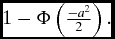 $1- \Phi \left(\frac{-a^2}{2}\right).$
The second period incumbent will be moderate if the first period incumbent is either retained or replaced by a challenger who turns out to be moderate. All told, then, given a first period moderate, the probability of a second period moderate is
 \begin{equation*}
1-\Phi \left(\frac{-a^2}{2}\right) + p\Phi \left(\frac{-a^2}{2}\right).
\end{equation*}
Second, suppose the first period incumbent is extreme. She is retained with probability
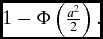 $1- \Phi \left(\frac{a^2}{2}\right).$
In this case, the second period incumbent can only be moderate if the first period incumbent is replaced and the challenger turns out to be moderate. This means that, given a first period extremist, the probability of a second period moderate is
 \begin{equation*}
p\Phi \left(\frac{a^2}{2}\right).
\end{equation*}
Hence, the overall probability that the second period incumbent is moderate with an uninformed voter is
 \begin{eqnarray*}
\eqcellsep\eqcellsep p\left[1-\Phi \left(\frac{-a^2}{2}\right) + p\Phi \left(\frac{-a^2}{2}\right) \right]\\
\eqcellsep\eqcellsep\quad +\, (1-p)p\Phi \left(\frac{a^2}{2}\right) <p + (1-p)p.
\end{eqnarray*}
This makes it clear that, if politician behavior does not respond to anticipated voter behavior, then the voter is indeed better off having more information about policy choices.
Voter Rationality without Strategic Politicians
By a similar analysis, in the model of fail-to-filter voters, for a fixed action by extremists,
 $a \not= 0$
, the probability the second period incumbent is a moderate is
 \begin{equation*}
p\left[1-\Phi \left(\frac{-a^2}{2\sigma }\right) + p\Phi \left(\frac{-a^2}{2\sigma }\right) \right] + (1-p)p\Phi \left(\frac{a^2}{2\sigma }\right),
\end{equation*}
where σ = 1 if the voter is rational and
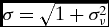 $\sigma = \sqrt{1 + \sigma ^2_\nu }$
if the voter irrationally fails to filter. It is straightforward to show that this probability is decreasing in σ. Hence, if politicians do not strategically respond to anticipated changes in voter behavior, voters are better off behaving rationally.
These results on the positive welfare implications of voter information and voter rationality with nonstrategic politicians show that the problems with the normative claims of the behavioral literature really do come from a failure to consider how politicians strategically adapt to changes in voter behavior.
CONCLUSION
An important debate in political behavior asks whether voters are sufficiently competent—i.e., informed or rational—to support standard normative defenses of democracy. Using two formal models, we show that the evidence offered by this literature (on both sides) simply does not speak to the normative concerns that motivate the papers. Our central point is that governance outcomes are the result of an interaction between politicians and voters, and thus one cannot reach conclusions about democratic performance by evaluating voter competence. Indeed, in our models we show that sometimes increased voter competence improves voter welfare and sometimes increased voter incompetence improves voter welfare.
We want to reemphasize that our point is not that, relative to the status quo, democratic performance would clearly be better or clearly be worse were voters less informed or less rational. In our view, the lesson to be drawn from our models is that decontextualized facts about voter characteristics simply do not have any normative implications for democracy one way or the other.
That said, we do not want to suggest that there is no way forward for empirical scholars who want to probe questions of democratic performance. Instead, we want to argue that the kind of work that does so focuses not on voters in isolation, but on elections as an interaction of voters and politicians within an institutional context. There are two benefits of this sort of approach. First, by focusing on outputs of, rather than inputs to, the electoral process, it avoids the problems we have highlighted for the behavior literature. Second, by focusing on facts about the institutional environment, rather than what may be unalterable properties of the electorate, it offers the possibility of yielding results with some practical implications for improving governance outcomes.
The existing empirical literature on political agency has made progress on these goals in a variety of ways. For instance, consistent with models of electoral agency, several papers examine, in reduced form, how changes to various features of the institutional environment affect the quality of governance (Besley and Case Reference Besley and Case2003; de Janvry, Finan and Sadoulet Reference de Janvry, Finan and Sadoulet2012; Ferraz and Finan Reference Ferraz and Finan2011; Gagliarducci and Nannicini Reference Gagliarducci and Nannicini2013; Gordon and Huber Reference Gordon and Huber.2007). Other work doesn’t get all the way to an encompassing measure of democratic performance, but unpacks the extent to which the welfare effects of elections operate through incentives versus selection of good types (Alt, Bueno de Mesquita and Rose Reference Alt, Bueno de Mesquita and Rose2011; Gagliarducci and Nannicini Reference Gagliarducci and Nannicini2013; Gordon and Huber Reference Gordon and Huber.2007). Finally, Snyder and Strömberg (Reference Snyder and Strömberg2010) provide an analysis that both traces how changes in the strategic environment affect the interaction between voters and politicians—showing that changes in the media environment alter voter information and politician behavior—and estimates the effect of such changes on democratic performance—showing that policy outcomes change.
Of course, there remain open questions. One of the lessons of the numerical analyses reported in Figures 3 and 5 is that we should expect significant heterogeneity in the relationship between voter information (or rationality) and democratic performance as a function of factors such as the pool of candidates (θ and p), voter preferences (δ), and the amount of irrelevant information voters are forced to deal with (σν). Hence, in other settings, we might expect to find relationships that differ from those identified by Snyder and Strömberg (Reference Snyder and Strömberg2010). Much detailed empirical work remains to be done, in many contexts, to get a handle on this kind of heterogeneity.
But what distinguishes this political agency literature, in our view, from the behavioral literature that we have criticized is a focus on the interaction of voters and politicians. The behavioral literature estimates characteristics of voters and asserts that those characteristics are good or bad for democracy, by assumption. The empirical papers mentioned above, and the theoretical models that guide them, aren’t terribly concerned with any particular characteristic of the voters. Instead they are focused on how changes to the electoral environment affect the behavior of all of the actors in that environment and, ultimately, the policy outcomes that are the actual measure of democratic performance.
A PROOFS FOR POLICY-CHOICE MODEL
Proof of Proposition 1. Differentiate the left-hand side of Equation (3) to get the second derivative of extreme incumbent payoffs with respect to a:
 \begin{eqnarray*}
\eqcellsep\eqcellsep -2(1-\delta )-2\delta \phi (\overline{\pi }+a^2)\theta ^2(p+(1-p)4)\\
\eqcellsep\eqcellsep \quad-\,2a\delta \phi ^{\prime }(\overline{\pi }+a^2)2a\theta ^2(p+(1-p)4).
\end{eqnarray*}
We’d like this to be nonpositive for all a ∈ [0, θ]. Divide by 2 and use the fact that ϕ′(x) = −xϕ(x) to rewrite the second derivative as
 \begin{eqnarray*}
\eqcellsep\eqcellsep -(1-\delta )-\delta \phi (\overline{\pi }+a^2)\theta ^2(p+(1-p)4)\\
\eqcellsep\eqcellsep\quad +\,a\delta (\overline{\pi }+a^2)\phi (\overline{\pi }+a^2)2a\theta ^2(p+(1-p)4).
\end{eqnarray*}
Collect variables in the last term to get
 \begin{eqnarray*}
\eqcellsep\eqcellsep -(1-\delta )-\delta \phi (\overline{\pi }+a^2)\theta ^2(p+(1-p)4)\\
\eqcellsep\eqcellsep\quad +\,2a^2\delta (\overline{\pi }+a^2)\phi (\overline{\pi }+a^2)\theta ^2(p+(1-p)4).
\end{eqnarray*}
Factor the last two terms to get
 \begin{equation*}
-(1-\delta )-\delta \phi (\overline{\pi }+a^2)\theta ^2(p+(1-p)4)\left[1-2a^2(\overline{\pi }+a^2)\right].
\end{equation*}
Rearrange to get
 \begin{equation*}
\delta [1-\phi (\overline{\pi }+a^2)\theta ^2(p+(1-p)4)[1-2a^2(\overline{\pi }+a^2)]] \le 1,
\end{equation*}
or
 \begin{equation}
\delta \le \frac{1}{1-\phi (\overline{\pi }+a^2)\theta ^2(p+(1-p)4)\left[1-2a^2(\overline{\pi }+a^2)\right]}.
\end{equation}
 $\overline{\pi }\in [-\frac{\theta ^2}{2},\frac{\theta ^2}{2}]$
, the factor
 $\left[1-2a^2(\overline{\pi }+a^2)\right]$
is minimized at a = θ and
 $\overline{\pi }=0$
. Its value at the minimum is
 \begin{equation*}
1-2\theta ^4.
\end{equation*}
There are two cases, depending on the sign of this minimum.
-
1. If
$\theta \le \left(\frac{1}{2}\right)^{1/4}$
, then the factor in square brackets in inequality (6) is non-negative. This implies that the right-hand side of inequality (6) is greater than or equal to 1, and the bound is satisfied for all δ. -
2. If
$\theta \ge \left(\frac{1}{2}\right)^{1/4}$
, then the right-hand side of inequality (6) is less than 1. Since
$\frac{1}{1-x}$
is increasing in x, the worst case for this bound is when
is negative and large in absolute value. We have
\begin{equation*}
\phi (\overline{\pi }+a^2)\theta ^2(p+(1-p)4)[1-2a^2(\overline{\pi }+a^2)]
\end{equation*}
Thus the bound is satisfied if
\begin{eqnarray*}
\eqcellsep\eqcellsep {\phi (\overline{\pi }+a^2)\theta ^2(p+(1-p)4)[1-2a^2(\overline{\pi }+a^2)]} \\
\eqcellsep\eqcellsep\quad \ge \phi (\overline{\pi }+a^2)\theta ^2(p+(1-p)4)(1-2\theta ^4) \\
\eqcellsep\eqcellsep\quad \ge \frac{1}{\sqrt{2\pi }}\theta ^2(p+(1-p)4)(1-2\theta ^4).
\end{eqnarray*}
\begin{equation*}
\delta \le \frac{\sqrt{2\pi }}{\sqrt{2\pi }+(p+(1-p)4)\theta ^2(2\theta ^4-1)}.
\end{equation*}


▪
Proof of Proposition 2.
Separating
Start with the case of separating. As we’ve seen in the text, there is a separating equilibrium when the voter is informed if
 $\delta \le \frac{1}{5-3p}$
. Hence, all we need to do to establish this part of the result is to show an open set of parameter values, consistent with this condition, such that voter welfare is higher under the uninformed equilibrium than under the separating equilibrium.
The proof follows the following steps:
-
1. We start by showing that, for any θ and p, in the limit as δ → 0, the welfares are equal.
-
2. We then show that, for any θ, there is an open set of p such that, in the limit as δ → 0 the difference between the derivative of the uninformed welfare and the derivative of the informed welfare with respect to δ is positive.
-
3. Fix a θ that implies the second-order condition and a p in the open set just described. The limit result gives an interval (0, δ) on which the derivative of uninformed welfare strictly exceeds the derivative of informed welfare. And since we have studied δ → 0, we are in the case of a separating equilibrium.
-
4. The fundamental theorem of calculus then gives WU (p, δ, θ) > WI (p, δ, θ).
-
5. This plus continuity of the welfare and the derivative in (p, δ, θ) implies that there is an open ball where the uninformed welfare is higher than the separating equilibrium welfare.
It will be useful to have the following facts, all of which follow from direct calculation:
Lemma 2
-
1.
\begin{equation*}
\lim _{\delta \rightarrow 0} a_* = \theta .
\end{equation*}
-
2.
\begin{equation*}
a_*(\delta = 1) = 0.
\end{equation*}
-
3.
{\fontsize{7}{9}\selectfont{\begin{equation*}
\hspace*{-12pt}\frac{d a_*}{d \delta } = - \frac{\theta -a_* + a_*\phi \left(\frac{a_*^2}{2}\right) (p\theta ^2 + (1-p)4 \theta ^2)}{1-\delta + \delta \phi \left(\frac{a_*^2}{2}\right)(p\theta ^2 + (1-p)4 \theta ^2) - \frac{a_*^4}{2} \delta \phi \left(\frac{a_*^2}{2}\right)(p\theta ^2 + (1-p)4 \theta ^2)}.
\end{equation*}}}
-
4.
\begin{equation*}
\lim _{\delta \rightarrow 0 }\frac{d a_*}{d \delta } = -\theta ^3\phi \left(\frac{\theta ^2}{2}\right)(p + (1-p)4).
\end{equation*}


Proof.
-
1. As δ → 0, the equilibrium condition goes to θ − a * = 0.
-
2. At δ = 1, the equilibrium condition is
$$a_* \delta \phi \left(\frac{a_*^2}{2}\right)(p\theta ^2 + (1-p)4\theta ^2) = 0,$$
which requires a
* = 0. -
3. Follows from the implicit function theorem.
-
4. Follows from points 1 and 3.

▪
Recall that, in the case of a separating equilibrium, voter welfares are
 \begin{equation*}
W^I = -(1-p)((1-\delta )\theta ^2 + \delta (1-p)\theta ^2)
\end{equation*}
and
 \begin{eqnarray*}
W^U \eqcellsep = \eqcellsep - p\delta \Phi \left(\frac{-a_*^2}{2}\right)(1-p)\theta ^2 - (1-p)\\
\eqcellsep\eqcellsep\times\,\left( (1-\delta )a_*^2 + \delta \left(1- p\Phi \left(\frac{a_*^2}{2}\right)\right)\theta ^2\right).
\end{eqnarray*}
Statement 1 of Lemma 2 implies that both of these welfares have the limit − (1 − p)θ2 as δ → 0.
The next step is to calculate the derivatives of WI and WU with respect to δ,
 \begin{equation*}
\frac{\partial W^I}{\partial \delta } = p(1-p)\theta ^2,
\end{equation*}
 \begin{eqnarray}
\frac{\partial W^{U}}{\partial \delta } \eqcellsep \hspace*{-1pt}=\hspace*{-1pt} \eqcellsep - p \Phi \left(\frac{-a_{*}^{2}}{2}\right)(1-p)\theta^{2} \hspace*{-1pt}+\hspace*{-1pt} p\delta \phi \left(\frac{-a_{*}^2}{2}\right) a_{*} \frac{\partial a_{*}}{\partial \delta }(1\hspace*{-1pt}-\hspace*{-1pt}p)\theta^{2} \nonumber\\
\eqcellsep\eqcellsep -\,(1\hspace*{-1pt}-\hspace*{-1pt}p)\left[ -a_{*}^{2} \hspace*{-1pt}+\hspace*{-1pt}2(1-\delta )a_{*}\frac{\partial a_{*}}{\partial \delta } \hspace*{-1pt}+\hspace*{-1pt} \left(1- p\Phi \left(\frac{a_{*}^{2}}{2}\right)\right)\theta ^{2} \right.\nonumber\\
\eqcellsep\eqcellsep\left.-\, \delta p\phi \left(\frac{a_{*}^{2}}{2}\right)a_{*}\frac{\partial a_{*}}{\partial \delta }\theta^{2}\right] .
\end{eqnarray}
The derivative of WI is independent of δ. Taking the limit of the derivative of WU as δ → 0, we have
 \begin{eqnarray*}
\eqcellsep\eqcellsep\lim _{\delta \rightarrow 0} \frac{\partial W^U}{\partial \delta } = - p \Phi \left(\frac{-\theta ^2}{2}\right)(1-p)\theta ^2 -(1-p)\left[\vphantom{\frac{\theta ^2}{2}} -\theta ^2 +2\theta \right.\\
\eqcellsep\eqcellsep\qquad\left.\times\,\left(-\theta ^3\phi \left(\frac{\theta ^2}{2}\right)\left(p + (1-p)4\right)\right) + \left(1- p\Phi \left(\frac{\theta ^2}{2}\right)\right)\theta ^2\right] \\
\eqcellsep\eqcellsep\quad=(1-p)\theta ^2\left[-p\Phi \left(\frac{-\theta ^2}{2}\right)+1+2\theta ^2\phi \left(\frac{\theta ^2}{2}\right)\right.\\
\eqcellsep\eqcellsep\qquad\left.\times\,(p+(1-p)4)-1+p\Phi \left(\frac{\theta ^2}{2}\right)\right].
\end{eqnarray*}
Comparing, we have that
 $\lim _{\delta \rightarrow 0} \frac{\partial W^U}{\partial \delta } > \lim _{\delta \rightarrow 0} \frac{\partial W^I}{\partial \delta }$
if
 \begin{equation*}
-p\Phi \left(\frac{-\theta ^2}{2}\right) + 2\theta ^2\phi \left(\frac{\theta ^2}{2}\right)(p+(1-p)4) +p\Phi \left(\frac{\theta ^2}{2}\right) > p.
\end{equation*}
Using the fact that Φ( − x) = 1 − Φ(x) this can be rearranged:
 \begin{equation*}
p < \frac{4\theta ^2\phi \left(\frac{\theta ^2}{2}\right)}{1 -\Phi \left(\frac{\theta ^2}{2}\right)+3\theta ^2\phi \left(\frac{\theta ^2}{2}\right)}\equiv \underline{p}.
\end{equation*}
The right-hand side of this inequality is strictly positive. Hence,
 $\lim _{\delta \rightarrow 0} \frac{\partial W^U}{\partial \delta } > \lim _{\delta \rightarrow 0} \frac{\partial W^I}{\partial \delta }$
for all p with
 $0<p<\underline{p}$
.
This establishes that, for each
 $p<\underline{p}$
, there is a
 $\underline{\delta }(p)>0$
such that
 $\delta <\underline{\delta }(p)$
implies
 \begin{eqnarray*}
\eqcellsep\eqcellsep W^U(p,\delta ,\theta )-W^I(p,\delta ,\theta )\\
\eqcellsep\eqcellsep\quad = \int _0^\delta \frac{\partial W^U}{\partial \delta }(p,\tilde{\delta },\theta )-\frac{\partial W^I}{\partial \delta }(p,\tilde{\delta },\theta )\,d\tilde{\delta } > 0.
\end{eqnarray*}
Thus there exists a parameter vector (p, δ, θ) ∈ (0, 1)2 × (0, 1] such that WU (p, δ, θ) − WI (p, δ, θ) > 0. Since these functions are continuous, the inequality holds on an open set.
Pooling
Next consider the case of pooling, so
 $\delta > \frac{1}{5-3p}$
. Again, all we need to do to establish this part of the result is to show an open set of parameter values, consistent with this condition, such that voter welfare is higher under the uninformed equilibrium than under the pooling equilibrium. Our strategy is to define the function
 \begin{equation*}
H(p,\delta ,\theta ) = W^U(p,\delta ,\theta ) - W^I(p,\delta ,\theta )
\end{equation*}
and show that, for any (p, θ), it has two properties:
-
1. H has a strict local minimum at δ = 1 and
-
2. H(p, 1, θ) = 0.
Together, these properties show that for any (p, θ) there exists a
 $\overline{\delta }<1$
such that the welfares are ranked as we want them for
 $\delta \in (\overline{\delta },1)$
, which implies the result.
The uninformed welfare is as above. The informed welfare, for the case of a pooling equilibrium, is
 \begin{equation*}
W^I = -\delta (1-p)\theta ^2.
\end{equation*}
To show that H has a strict local minimum at δ = 1, we show that its first derivative is zero and its second derivative is strictly positive at δ = 1.
 \begin{equation*}
\frac{\partial H}{\partial \delta } = \frac{\partial W^U}{\partial \delta } - \frac{\partial W^I}{\partial \delta }.
\end{equation*}
Equation (7) gives
 $\frac{\partial W^U}{\partial \delta }$
. Substituting for δ = 1 and a
*(δ = 1) = 0 we have
 \begin{equation*}
\frac{\partial W^U}{\partial \delta }(p,1,\theta ) = -(1-p)\theta ^2.
\end{equation*}
Clearly,
 $\frac{\partial W^I}{\partial \delta } = -(1-p)\theta ^2$
. Thus,
 \begin{equation*}
\frac{\partial H}{\partial \delta }(p,1,\theta ) = 0.
\end{equation*}
Next consider the second derivative.
 \begin{equation*}
\frac{\partial ^2 H}{\partial \delta ^2} = \frac{\partial ^2 W^U}{\partial \delta ^2} - \frac{\partial ^2 W^I}{\partial \delta ^2}.
\end{equation*}
Clearly
 $\frac{\partial ^2 W^I}{\partial \delta ^2} =0$
. Taking the second derivative of the uninformed welfare we have
 \begin{equation*}
\frac{\partial ^2 W^U}{\partial \delta ^2}(p,1,\theta ) = 2 p(1-p)\theta ^2\phi (0)\left(\frac{\partial a_*}{\partial \delta }\right)^2.
\end{equation*}
This is strictly positive, as required, as long as
 $\frac{\partial a_*}{\partial \delta }\not= 0.$
From Lemma 2, at δ = 1 we have
 \begin{equation*}
\frac{d a_*}{d \delta }(p,1,\theta ) = - \frac{\theta }{\phi \left(0\right)\left(p\theta ^2 + (1-p)4 \theta ^2\right) } <0.
\end{equation*}
Now all that remains is to show that H(p, 1, θ) = 0. At δ = 1, informed welfare is − (1 − p)θ2. Substituting for δ = 1 and a *(δ = 1) = 0 in the uninformed welfare gives
 \begin{equation*}
W^U(p,1,\theta ) =- p \Phi \left(0\right)(1-p)\theta ^2 - (1-p) (1- p\Phi \left(0\right)\theta ^2 ).
\end{equation*}
Since Φ(0) = 1/2, this also reduces to − (1 − p)θ2, as required. ▪
Proof of Proposition 3. As we saw in the main text, the derivative of ex ante voter welfare with respect to the reelection standard is
 {\fontsize{7}{9}\selectfont{\begin{eqnarray*}
\eqcellsep\eqcellsep \frac{d W(\overline{\pi })}{d \overline{\pi }} = \overbrace{\delta p(1-p)\theta ^2 [\phi (\overline{\pi } + a_*(\overline{\pi })^2)-\phi (\overline{\pi })]}^{\mbox{Direct Effect}} \\
\eqcellsep\eqcellsep\quad \overbrace{- \frac{d a_*(\overline{\pi })}{d\overline{\pi }}\left[\underbrace{2(1-\delta )(1-p)a_*(\overline{\pi })}_{\mbox{First Period Effect}} - \underbrace{ \delta 2a_*(\overline{\pi })p(1-p)\theta ^2\phi (\overline{\pi } + a_*(\overline{\pi })^2)}_{\mbox{Second Period Effect}}\right]}^{\mbox{Indirect Effects}}.
\end{eqnarray*}}}
At the equilibrium,
 $\overline{\pi }_*=- (\overline{\pi }_*+a_*(\overline{\pi }_*)^2)$
, so symmetry of the normal pdf implies
 $\phi (\overline{\pi }_* + a_*(\overline{\pi }_*)^2)-\phi (\overline{\pi }_*)=0$
. Thus, starting from an equilibrium, the direct effect is 0. (This is a manifestation of the envelope theorem.) Hence, the overall effect on welfare is determined by a comparison of the two indirect effects. Thus, some small change in
 $\overline{\pi }$
away from the equilibrium value will yield an increase in voter welfare unless one of two conditions holds:
-
1.
$\frac{d a_*(\overline{\pi }_*)}{d\overline{\pi }} = 0$
or -
2.
$\delta = \frac{1}{1+p\theta ^2 \phi (\overline{\pi }_* +a_*(\overline{\pi }_*)^2)}$


Applying the implicit function theorem to Equation (3) gives the effect of a change in the voter’s cutoff rule on the extreme incumbent’s action:
 {\fontsize{8}{10}\selectfont{\begin{eqnarray*}
\hspace*{-8pt}\eqcellsep\eqcellsep \frac{d a_*}{d \overline{\pi }} = \\
\hspace*{-8pt}\eqcellsep\eqcellsep \quad-\, \frac{-2a_* \delta \phi ^{\prime }(\overline{\pi }+a_*^2) (p \theta ^2 +(1-p) 4 \theta ^2) }{-2(1-\delta ) -(2\delta \phi (\overline{\pi } + a_*^2) + 4a_*^2\delta \phi ^{\prime }(\overline{\pi } + a_*^2))(p \theta ^2 +(1-p) 4 \theta ^2) } .
\end{eqnarray*}}}
Since a
* > 0, the only way for this derivative to be zero is for
 $\phi ^{\prime }(\overline{\pi } + a_*^2) =0$
. This is only true if
 $a_*^2 = -\overline{\pi }$
. But the equilibrium
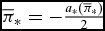 $\overline{\pi }_* = -\frac{a_*(\overline{\pi }_*)}{2}$
, so
 $\frac{d a_*(\overline{\pi }_*)}{d\overline{\pi }} \not= 0$
.
All that’s left is to consider the second condition. The equilibrium condition (4) implicitly defines an a *(δ). The condition for voter welfare not responding to a change in the voting rule,
 \begin{equation*}
\delta = \frac{1}{1+p\theta ^2 \phi (\overline{\pi }_* +\hat{a}^2)},
\end{equation*}
implicitly defines an
 $\hat{a}(\delta )$
.
Intuitively, to show that the second condition doesn’t hold generically, we will show that, at any
 $\hat{\delta }$
where
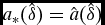 $a_*(\hat{\delta })=\hat{a}(\hat{\delta })$
, the graph of a
* is steeper than the graph of
 $\hat{a}$
. Thus they can cross at most once, so the set where the condition holds is closed and has measure zero.
Our formal results use the following ideas from differential topology. Specializing Theorem 8.8 of Lee (Reference Lee2003, 182) yields
Theorem 1 (Constant-Rank Level Set Theorem)
Let M be an open subset of
 $\mathbb {R}^n$
and let
 $f:M\rightarrow \mathbb {R}$
be a smooth (i.e., infinitely many times continuously differentiable) map with the rank of Df(a) constant at k. Each level set of f is a closed submanifold of co-dimension k in M.
We will apply this result to the map
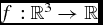 $f:\mathbb {R}^3\rightarrow \mathbb {R}$
given by
 \begin{equation*}
f(p,\delta ,\theta )=\delta +\delta p\theta ^2\phi \left(\frac{a_*(p,\delta ,\theta )^2}{2}\right).
\end{equation*}
Differentiate to get
 \begin{equation*}
\frac{\partial\, f}{\partial \delta }=1+p\theta ^2 \phi \left(\frac{a_*^2}{2}\right) -\delta p\theta ^2 \frac{a_*^3}{2}\phi \left(\frac{a_*^2}{2}\right) \frac{\partial a_*}{\partial \delta }.
\end{equation*}
Since a * is decreasing in δ, this derivative is positive. By the rank-nullity theorem, this implies that Df has rank 1 for all (p, δ, θ). Thus condition 2 above can hold only on a two-dimensional submanifold, a closed set of measure zero. ▪
Proof of Proposition 4. It suffices to show that welfare is increasing in σ at σ = 1. Differentiating, we have
 \begin{eqnarray*}
\frac{d W^U}{d\sigma }(\sigma =1)\eqcellsep = \eqcellsep -2(1-\delta )(1-p)a_* \frac{\partial a_*}{\partial \sigma }\\
\eqcellsep\eqcellsep -\, 2\delta p(1-p)\theta ^2\phi \left(\frac{-a_*^2}{2}\right)\left(\frac{a_*^2}{2} - \frac{2a_*\frac{\partial a_*}{\partial \sigma }}{2}\right).
\end{eqnarray*}
Rearrange to see that welfare is increasing in σ at σ = 1 if
 \begin{equation}
p < \frac{-(1-\delta ) \frac{\partial a_*}{\partial \sigma }}{\delta \theta ^2\phi \left(\frac{-a_*^2}{2}\right)\left(\frac{a_*}{2} - \frac{\partial a_*}{\partial \sigma }\right)}.
\end{equation}
Lemma 3
Let
 $\overline{k}=\frac{\theta -\sqrt{2}}{2}$
. There is a
 $\overline{\delta }>0$
such that, if
 $0<\delta < \overline{\delta }$
, and
 $0<k<\overline{k}$
, then for every p ∈ [0, 1], at σ = 1,
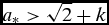 $a_* > \sqrt{2} + k$
.
Proof. From Lemma 2, there exists a
 $\overline{\delta }$
such that
 $\delta < \overline{\delta }$
implies θ − a
* < k. Together, these imply that
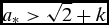 $a_* > \sqrt{2} + k$
. ▪
Lemma 4
Suppose
 $0<\delta <\overline{\delta }$
. Then, for each p and θ, there are
 $\underline{\ell }$
and
 $\overline{\ell }<0$
such that
 \begin{equation*}
\underline{\ell }\le \frac{\partial a_*}{\partial \sigma }\le \overline{\ell }.
\end{equation*}
Proof. First we argue that
 $\frac{\partial a_*}{\partial \sigma }$
is bounded. Recall that a
* is defined as the solution to Equation (4). We are going to construct a function α* on a larger domain that we can use to find bounds for a
* and its derivatives. Let
 $\mathcal {D} = (-\beta ,1+\beta )\times (1-2\gamma ,1+2\gamma )$
, where β > 0 and γ > 0 are small enough that for all
 $(\delta ,\sigma ) \in \mathcal {D}$
,
 \begin{equation*}
1 - \delta + \delta (p\theta ^2 + (1-p)4 \theta ^2)\frac{1}{\sigma }\phi \left(\frac{a^2}{2\sigma }\right)\left( \frac{2\sigma ^2 -a^4}{2\sigma ^2}\right) > 0
\end{equation*}
for all a ∈ [0, θ].
Define α* implicitly as the solution to Equation (4) on domain
 $\mathcal {D}$
. The implicit function theorem tell us that α* is continuously differentiable in δ and σ. Because
 $\frac{\partial \alpha _*}{\partial \sigma }$
is continuous on the compact set
 $[0,1]\times [1-\gamma ,1+\gamma ]\subset \mathcal {D}$
, it is bounded on that set. But restricting the function to a subset of its domain cannot make it unbounded.
Next we show that, for
 $\delta <\overline{\delta }$
, the upper bound is negative and bounded away from 0. From the implicit function theorem, we can write
 \begin{eqnarray}
\frac{\partial a_*}{\partial \sigma }(\sigma = 1) = \frac{a_*\delta \left(p\theta ^2 + (1-p)4\theta ^2\right)\phi \left(\frac{a_*^2}{2}\right)\left(\frac{4-a_*^4}{4}\right)}{1 - \delta + \delta (p\theta ^2 + (1-p)4 \theta ^2)\phi \left(\frac{a_*^2}{2}\right)\left( \frac{2 -a_*^4}{2}\right)}.\nonumber\\
\end{eqnarray}
As δ → 0, the denominator in Equation (9) goes to 1 and, as shown by Lemma 3, the numerator is negative. Thus, for δ sufficiently small, the derivative is negative. Moreover, we can give an upper bound on the derivative.
 \begin{eqnarray*}
\frac{\partial a_*}{\partial \sigma }(\sigma = 1) \eqcellsep=\eqcellsep \frac{a_*\delta (p\theta ^2 + (1-p)4\theta ^2)\phi \left(\frac{a_*^2}{2}\right)\left(\frac{4-a_*^4}{4}\right)}{1 - \delta + \delta (p\theta ^2 + (1-p)4 \theta ^2)\phi \left(\frac{a_*^2}{2}\right)\left( \frac{2 -a_*^4}{2}\right)}\\
\eqcellsep \le\eqcellsep a_*\delta (p\theta ^2 + (1-p)4\theta ^2)\phi \left(\frac{a_*^2}{2}\right)\left(\frac{4-a_*^4}{4}\right)\\
\eqcellsep<\eqcellsep (\sqrt{2} + \overline{k}) \delta \theta ^2\phi \left(\frac{\theta ^2}{2}\right) \left(\frac{4-(\sqrt{2}+\overline{k})^4}{4}\right) \equiv \delta \overline{\ell },
\end{eqnarray*}
where the first inequality comes from maximizing the denominator and the second inequality comes from using Lemmas 2 and 3 to minimize the absolute value of the numerator.
It is immediate from Lemma 3 that
 $\overline{\ell } < 0$
. ▪
Using Lemmas 3 and 4, we have
 \begin{eqnarray*}
\frac{-(1-\delta ) \frac{\partial a_*}{\partial \sigma }}{\delta \theta ^2\phi \left(\frac{-a_*^2}{2}\right)\left(\frac{a_*}{2} - \frac{\partial a_*}{\partial \sigma }\right)} &{>}& \frac{-(1-\delta )\delta \overline{\ell }}{\delta \theta ^2\phi \left(\frac{-a_*^2}{2}\right)\left(\frac{a_*}{2} - \frac{\partial a_*}{\partial \sigma }\right)}\\
&{>}& \frac{-(1-\delta )\overline{\ell }}{\theta ^2\left(\frac{1}{\sqrt{2\pi }}\right)\left(\frac{\theta }{2} - \underline{\ell }\right)}\\
&{>}&0.
\end{eqnarray*}
If δ satisfies
 $0<\delta <\overline{\delta }$
and p satisfies
 \begin{equation*}
0<p<\frac{-(1-\delta )\overline{\ell }}{\theta ^2\left(\frac{1}{\sqrt{2\pi }}\right)\left(\frac{\theta }{2}-\underline{\ell }\right)},
\end{equation*}
then Condition 8 is satisfied, as required. ▪
B THE EFFORT GAME
B.1 Equilibrium in the Effort Game
We start by characterizing equilibria with informed voters.
If the voter is informed, then, following action a and outcome π = f(a, θ) + ε, his posterior belief about the probability that
 $\theta _I = \overline{\theta }$
is
 \begin{equation*}
\Pr (\theta _I = \overline{\theta }|\pi ,a) = \frac{p \phi (\pi - f(a, \overline{\theta }))}{p\phi (\pi - f(a,\overline{\theta })) + (1-p)\phi (\pi -f(a , \underline{\theta }) )}.
\end{equation*}
The voter reelects if that posterior is greater than or equal to his belief that the challenger is high ability (p), which means the voter reelects if and only if
 \begin{equation*}
\frac{\phi (\pi - f(a,\overline{\theta }))}{\phi (\pi - f(a,\underline{\theta }))} \ge 1.
\end{equation*}
By the MLRP, the left-hand side is increasing in π so the voter uses a simple cutoff rule, reelecting if and only if
 \begin{equation*}
\pi \ge \frac{f(a,\overline{\theta })+f(a,\underline{\theta })}{2}\equiv \hat{\pi }(a).
\end{equation*}
Given this best response by the voter, the incumbent solves
 \begin{eqnarray*}
\eqcellsep\eqcellsep \max _a \delta [ 1-p\Phi (\hat{\pi }(a)-f(a,\overline{\theta }))-(1-p)\Phi (\hat{\pi }(a)-f(a,\underline{\theta }))]\\
\eqcellsep\eqcellsep\quad -\,(1-\delta )c(a).
\end{eqnarray*}
In a pure-strategy equilibrium, the incumbent’s action aI * is characterized by the first-order condition:
 \begin{eqnarray}
\eqcellsep\eqcellsep\delta \phi \left(\frac{f(a^I_*,\overline{\theta })-f(a^I_*,\underline{\theta })}{2}\right)\left[p\left(\frac{\partial\, f}{\partial a}(a^I_*,\overline{\theta })-\frac{d\hat{\pi }}{d a}(a^I_*)\right)\right.\nonumber\\
\eqcellsep\eqcellsep\quad\left.+\,(1-p)\left(\frac{\partial\, f}{\partial a}(a^I_*,\underline{\theta })-\frac{d\hat{\pi }}{d a}(a^I_*)\right)\right]\le (1-\delta ) c^{\prime }(a^I_*), \nonumber\\
\end{eqnarray}
with equality if aI * > 0.
Next consider equilibrium with an uninformed voter. If the voter observes outcome π and conjectures that the incumbent took action
 $\tilde{a}$
, his posterior belief about the probability that
 $\theta _I = \overline{\theta }$
is
 \begin{equation*}
\Pr (\theta _I = \overline{\theta }|\pi ,\tilde{a}) = \frac{p \phi (\pi - f(\tilde{a} , \overline{\theta }))}{p\phi (\pi - f(\tilde{a},\overline{\theta })) + (1-p)\phi (\pi -f(\tilde{a}, \underline{\theta }))}.
\end{equation*}
The voter reelects if that posterior is greater than or equal to his belief that the challenger is high ability (p), which means the voter reelects if and only if:
 \begin{equation*}
\frac{\phi (\pi - f(\tilde{a},\overline{\theta }))}{\phi (\pi - f(\tilde{a},\underline{\theta }))} \ge 1.
\end{equation*}
By the MLRP, the left-hand side is increasing in π so the voter uses a simple cutoff rule, reelecting if and only if
 \begin{equation*}
\pi \ge \frac{f(\tilde{a},\overline{\theta })+f(\tilde{a},\underline{\theta })}{2}\equiv \overline{\pi }(\tilde{a}).
\end{equation*}
Note an important difference between the cutoffs
 $\hat{\pi }$
and
 $\overline{\pi }$
. The informed voter uses a cutoff
 $\hat{\pi }$
that is a function of the actual action taken by the incumbent. The uninformed voter uses a cutoff
 $\overline{\pi }$
that does not track the incumbent’s action as she deviates from what is expected. This difference leads to a different first-order condition.
If the voter uses a cutoff rule
 $\overline{\pi }$
, then the incumbent’s best response solves
 \begin{eqnarray*}
\eqcellsep\eqcellsep \max _a \delta [ 1- p\Phi (\overline{\pi } - f(a, \overline{\theta })) - (1-p)\Phi (\overline{\pi } - f(a , \underline{\theta }))]\\
\eqcellsep\eqcellsep\quad - \,(1-\delta )c(a).
\end{eqnarray*}
In a pure strategy equilibrium, the equilibrium action aU
* is given by the first-order condition with
 $\overline{\pi }$
held constant at
 $\overline{\pi }_*(a^U_*)$
,Footnote
13
 \begin{eqnarray}
\eqcellsep\eqcellsep \delta \phi \left(\frac{f(a^U_*,\overline{\theta })-f(a^U_*,\underline{\theta })}{2}\right)\left[p\frac{\partial\, f}{\partial a}(a^U_*,\overline{\theta })+(1-p)\frac{\partial\, f}{\partial a}(a^U_*,\underline{\theta })\right]\nonumber\\
\eqcellsep\eqcellsep\quad =(1-\delta ) c^{\prime }(a^U_*).
\end{eqnarray}
B.2 Comparing Informed and Uninformed Voter Welfare
The left-hand side (LHS) of inequality (10) is less than the LHS of Equation (11), suggesting the following result:
Lemma 5 The first period action in the effort game is higher when the voter is uninformed than when the voter is informed: aU * > aI *.
Proof. First observe that
 \begin{equation*}
\frac{d \hat{\pi }}{d a}(a)=\frac{1}{2}\left(\frac{\partial\, f}{\partial a}(a,\overline{\theta })+\frac{\partial\, f}{\partial a}(a,\underline{\theta })\right)>0,
\end{equation*}
where the inequality follows from monotonicity of f.
Define the functions
 \begin{eqnarray*}
\eqcellsep\eqcellsep h^I(a)=\delta \phi \left(\frac{f(a,\overline{\theta })-f(a,\underline{\theta })}{2}\right)\left[p\left(\frac{\partial\, f}{\partial a}(a,\overline{\theta })-\frac{d\hat{\pi }}{d a}(a)\right)\right.\nonumber\\
\eqcellsep\eqcellsep\quad\left.+\,(1-p)\left(\frac{\partial\, f}{\partial a}(a,\underline{\theta })-\frac{d\hat{\pi }}{d a}(a)\right)\right]-(1-\delta ) c^{\prime }(a)
\end{eqnarray*}
and
 \begin{eqnarray*}
\hspace*{-6pt}\eqcellsep\eqcellsep\delta \phi \left(\frac{f(a,\overline{\theta })-f(a,\underline{\theta })}{2}\right)\left[p\left(\frac{\partial\, f}{\partial a}(a,\overline{\theta })\right)+(1-p)\left(\frac{\partial\, f}{\partial a}(a,\underline{\theta })\right)\right]\nonumber\\
\hspace*{-6pt}\eqcellsep\eqcellsep\quad-\,(1-\delta ) c^{\prime }(a).
\end{eqnarray*}
Let
 $H:\mathbb {R}_+\times \lbrace 0,1\rbrace$
be given by
 \begin{equation*}
H(a,\chi )=\chi h^U(a)+(1-\chi )h^I(a).
\end{equation*}
The observation at the start of the proof implies that, for all a, we have
 \begin{equation*}
\frac{d h^U}{d a}(a)>\frac{d h^I}{d a}(a),
\end{equation*}
so
 $\frac{\partial H}{\partial a}$
is increasing in χ. Furthermore, H is continuous in a because f and c are continuously differentiable. Thus Theorem 1 of Milgrom and Roberts (Reference Milgrom and Roberts1994) implies the result. ▪
It is clear that first period voter welfare is increasing in the incumbent’s action. So the voter’s overall welfare is increasing in the action, for any discount factor, if the second period welfare is (weakly) increasing in the action. We now show that this holds if the action and type are weak complements:
 \begin{equation*}
\frac{\partial\, f}{\partial a}(a,\overline{\theta })\ge \frac{\partial\, f}{\partial a}(a,\underline{\theta }) \ \ \ \mbox{ for all }a\ge 0.
\end{equation*}
Note that this condition is satisfied for both the additive model in Ashworth (Reference Ashworth2005) and the multiplicative model in Ashworth and Bueno de Mesquita (Reference Ashworth and Bueno de Mesquita2006).
Lemma 6 Suppose a * is the first period action in the effort game (with either an informed or uninformed voter). Second period voter welfare is
 \begin{equation*}
p(1\hspace*{-1pt}-\hspace*{-1pt}p)\Phi \left(\frac{f(a_*,\overline{\theta })\hspace*{-1pt}-\hspace*{-1pt}f(a_*,\underline{\theta })}{2}\right)(f(0,\overline{\theta })\hspace*{-1pt}-\hspace*{-1pt}f(0,\underline{\theta }))\hspace*{-1pt}+\hspace*{-1pt}f(0,\underline{\theta }).
\end{equation*}
Proof. Second period welfare depends on whether the voter is informed or not only through the effect of information on the equilibrium action. In the informed case, the voter forms his posterior belief directly using the actual action. In the uninformed case, the voter forms his posterior belief using his conjecture about the incumbents’s action. Crucially, this conjecture is correct in equilibrium. Thus, whatever the informational environment, second period welfare, given action a *, is the same.
Whichever politician is in office in the second period will choose a = 0. Thus second period voter welfare is
 \begin{equation*}
\Pr (\theta _2=\overline{\theta }\mid a_*) (f(0,\overline{\theta })-f(0,\underline{\theta }))+f(0,\underline{\theta }).
\end{equation*}
To calculate this probability, observe that there are three ways to get a high type in office in the second period. The incumbent can be high type and win reelection, the incumbent can be a high type who is replaced by a high type, or the incumbent can be a low type who is replaced by a high type. Summing the probabilities of these three events gives
 \begin{eqnarray*}
\hspace*{-7pt}\eqcellsep\eqcellsep p\left[1\hspace*{-2pt}-\hspace*{-2pt}\Phi \left(\frac{f(a_*,\underline{\theta })-f(a_*,\overline{\theta })}{2}\right)\right]\hspace*{-2pt}+\hspace*{-2pt}p\Phi \left(\frac{f(a_*,\underline{\theta })-f(a_*,\overline{\theta })}{2}\right)\\
\hspace*{-7pt}\eqcellsep\eqcellsep\quad\times\, p+(1-p)\Phi \left(\frac{f(a_*,\overline{\theta })-f(a_*,\underline{\theta })}{2}\right)p,
\end{eqnarray*}
which simplifies to
 \begin{equation*}
p(1-p)\Phi \left(\frac{f(a_*,\overline{\theta })-f(a_*,\underline{\theta })}{2}\right).
\end{equation*}
▪
The expression for second period voter welfare is increasing in
 $f(a_*,\overline{\theta })-f(a_*,\underline{\theta })$
. And that is weakly increasing in a
* if and only if
 \begin{equation*}
\frac{\partial\, f}{\partial a}(a,\overline{\theta })-\frac{\partial\, f}{\partial a}(a,\underline{\theta })\ge 0,
\end{equation*}
which is exactly the statement that a and θ are weak complements. Thus we have the following:
Corollary 1 Suppose effort and type are weak complements in the effort game. Then second period voter welfare is weakly increasing in the equilibrium first period action.
Lemma 5 and Corollary 1 immediately give a result that is even stronger than the result for the policy game in Proposition 2.
Proposition 5 Suppose effort and type are weak complements in the effort game. Then voter welfare is strictly higher when the voter is uninformed than when the voter is informed.
B.3 Irrational Voters Can Yield Higher Welfare
Next we show that irrational voters can yield higher welfare than rational voters in the effort choice game. As before, let
 $a_*(\overline{\pi })$
be a best response to an arbitrary cutoff rule. It again suffices to show that the derivative of voter welfare with respect to the cutoff rule is not zero.
Voter welfare at an arbitrary cutoff rule
 $\overline{\pi }$
is
 $W(\overline{\pi })$
given by
 \begin{eqnarray*}
\eqcellsep\eqcellsep (1-\delta )a_*(\overline{\pi }) + \delta \left ({[}p [ 1-\Phi (\overline{\pi } -f{(}a_*(\overline{\pi }),\overline{\theta }{)})(1-p)] \right.\nonumber\\
\eqcellsep\eqcellsep\left.\quad+\, {}(1-p)\Phi (\overline{\pi } -f{(}a_*(\overline{\pi }),\underline{\theta }{)}p{]}(f(0,\overline{\theta })-f(0,\underline{\theta })) \right.\nonumber\\
\eqcellsep\eqcellsep\left.\quad+\, f(0,\underline{\theta })\right ).
\end{eqnarray*}
At the equilibrium, the envelope theorem and symmetry of the normal density imply
 \begin{eqnarray*}
\eqcellsep\eqcellsep\frac{\partial W}{\partial \overline{\pi }} = \left[(1-\delta )+ \delta p(1-p)\phi \left(\frac{f(a_*,\underline{\theta })-f(a_*,\overline{\theta })}{2}\right)\right.\nonumber\\
\eqcellsep\eqcellsep\quad\left.\times\,\left(\frac{\partial\, f}{\partial a}(a_*,\overline{\theta })-\frac{\partial\, f}{\partial a}(a_*,\underline{\theta })\right)(f(0,\overline{\theta })-f(0,\underline{\theta }))\right]\frac{\partial a_*}{\partial \overline{\pi }}.
\end{eqnarray*}
If action and type are weak complements, then the bracketed factor is positive, so it suffices to show that a
* is not constant in
 $\overline{\pi }$
at the equilibrium cutoff rule. Implicitly differentiating, this is true if and only if
 \begin{equation*}
p\frac{\partial\, f}{\partial a}(a_*,\overline{\theta })=(1-p)\frac{\partial\, f}{\partial a}(a_*,\underline{\theta }).
\end{equation*}
Define the function
 $g:(0,1)^2\rightarrow \mathbb {R}$
by
 \begin{equation*}
g(p,\delta )=p\frac{\partial\, f}{\partial a}{(}a_*(p,\delta ),\overline{\theta }{)}-(1-p)\frac{\partial\, f}{\partial a}{(}a_*(p,\delta ),\underline{\theta }{)}.
\end{equation*}
The Jacobian matrix is
 {\fontsize{7}{9}\selectfont{\begin{eqnarray*}
\eqcellsep\eqcellsep Dg(p,\delta )\\
\eqcellsep\eqcellsep\quad =\left(\begin{array}{c}\frac{\partial\, f}{\partial a}(a_*,\overline{\theta })+\frac{\partial\, f}{\partial a}(a_*,\underline{\theta })+\left(p\frac{\partial ^2 f}{\partial a^2}(a_*,\overline{\theta })-(1-p)\frac{\partial ^2 f}{\partial a^2}(a_*,\underline{\theta })\right)\frac{\partial a_*}{\partial p} \\[6pt]
\left(p\frac{\partial ^2 f}{\partial a^2}(a_*,\overline{\theta })-(1-p)\frac{\partial ^2 f}{\partial a^2}(a_*,\underline{\theta })\right)\frac{\partial a_*}{\partial \delta } \end{array} \right).
\end{eqnarray*}}}
The implicit function theorem implies that
 $\frac{\partial a_*}{\partial \delta }\ne 0$
. This means the only way that
 $\frac{\partial g}{\partial \delta }$
can be zero is if
 \begin{equation*}
\left(p\frac{\partial ^2 f}{\partial a^2}(a_*,\overline{\theta })-(1-p)\frac{\partial ^2 f}{\partial a^2}(a_*,\underline{\theta })\right)=0.
\end{equation*}
But then
 \begin{equation*}
\frac{\partial g}{\partial p}=\frac{\partial\, f}{\partial a}(a_*,\overline{\theta })+\frac{\partial\, f}{\partial a}(a_*,\underline{\theta })>0.
\end{equation*}
Thus Dg(p, δ) has rank 1 for all (p, δ), and the constant-rank level set theorem implies the following:
Proposition 6 In the effort game, except possibly on a closed set of measure zero, there exists an irrational reelection rule that, when best responded to, yields higher voter welfare than the equilibrium welfare.
B.4 Voters Who Fail to Filter
As before, consider a model that is virtually identical to the effort model with an uninformed voter, with the exception that the voter’s welfare in period t is now a function of observable events not affected by the politician in office (ν t ) in addition to the three factors from the previous model—the action (at ), the politician’s type (θ t ), and unobservable noise (ε t ). Each ν is observable and drawn independently (of all other random variables) from a normal distribution with mean 0 and variance σ2 ν.
As in the policy choice model in the text, it suffices to show that voter welfare is increasing in σ at σ = 1. If action and type are weak complements, Corollary 1 implies that welfare is increasing in σ if and only if a * is increasing in σ.
An argument identical to that leading to Equation (11) shows that a * is given by
 \begin{eqnarray*}
\eqcellsep\eqcellsep \delta \left(\frac{1}{\sigma }\right)\phi \left(\frac{f(a_*,\underline{\theta })-f(a_*,\overline{\theta })}{2\sigma }\right)\left[ p\frac{\partial\, f}{\partial a}(a_*,\overline{\theta }) \right.\nonumber\\
\eqcellsep\eqcellsep\quad\left.+\,(1-p) \frac{\partial\, f}{\partial a}(a_*,\underline{\theta })\right]= (1-\delta ) c^{\prime }(a_*).
\end{eqnarray*}
Implicitly differentiate to see that
 $\frac{\partial a_*}{\partial \sigma }$
is positive if and only if
 \begin{equation*}
\frac{d}{d\sigma }\left[\frac{1}{\sigma }\phi \left(\frac{f(a_*,\underline{\theta })-f(a_*,\overline{\theta })}{2\sigma }\right)\right]>0,
\end{equation*}
or
 \begin{equation*}
-\hspace*{-1pt}\frac{1}{\sigma ^2}\phi \left(\frac{f(a_*,\underline{\theta })-f(a_*,\overline{\theta })}{2\sigma }\right)\left[1\hspace*{-1pt}-\hspace*{-1pt}\frac{(f(a_*,\underline{\theta })-f(a_*,\overline{\theta }))^2}{2\sigma ^2}\right]\hspace*{-1pt}>\hspace*{-1pt}0,
\end{equation*}
which is positive at σ = 1 if and only if
 $f(a_*,\overline{\theta })-f(a_*,\underline{\theta }) > 2$
. If action and type are weak complements, then a sufficient condition for this inequality is
 $f(0,\overline{\theta })-f(0,\underline{\theta })>2$
.
Proposition 7
Suppose action and type are weak complements and
 $f(0,\overline{\theta })-f(0,\underline{\theta })>2$
. Then there exist fail-to-filter voters who attain higher welfare than rational voters.
C SIMULATIONS
The goal is to show our irrationality results for nonmarginal δ. To do so, we set δ = 0.15 and θ E = 1.9.
We compute the incumbent’s equilibrium action using Newton’s method.Footnote 14 Figure 6 shows the incumbent’s objective function (given that the incumbent expects the voter to use the equilibrium reelection rule, derived from computation of the equilibrium action). On the horizontal axis, we also plot the computed equilibrium action. The fact that the maximum of the objective and the computed equilibrium action coincide shows that the computations are in fact identifying the equilibrium for these parameter values.
FIGURE 6.

Having validated that we can compute an equilibrium for these parameter values, Figure 7 shows that for many of them, the voter is better off if he irrationally fails to filter.
FIGURE 7.

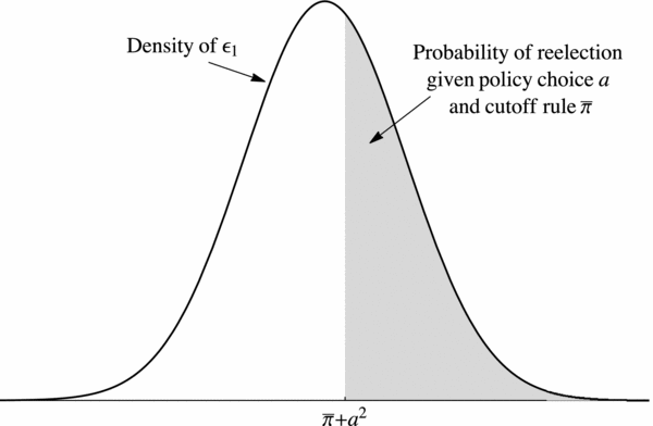
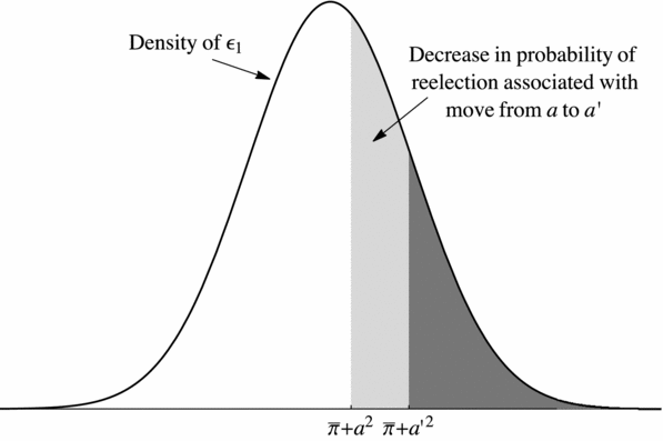
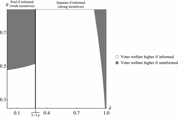
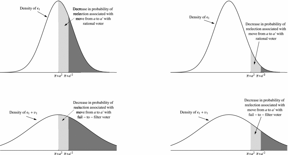
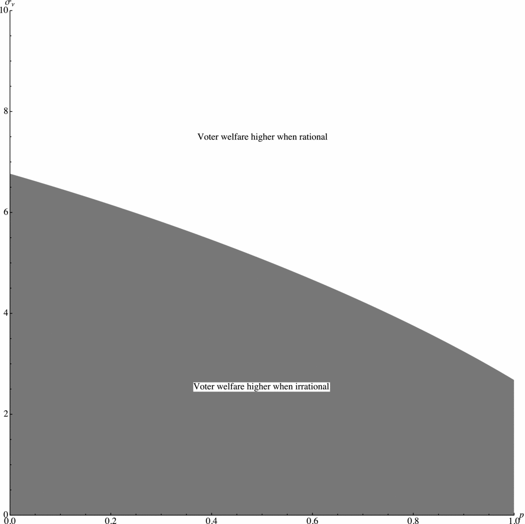
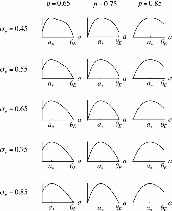
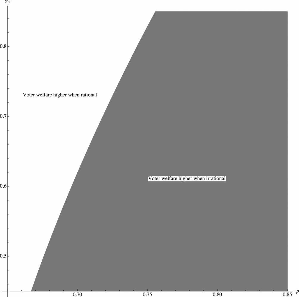



Comments
No Comments have been published for this article.