NOMENCLATURE
Symbols
- a
semi-major axis, km
- d
ground track drift distance, km
- E
Earth (subscript)
- e
eccentricity
- h
altitude, km
- i
inclination, degree
 ${J_2}$
Earth’s oblateness coefficient
- L
lunar (subscript)
- M
perturbed mean motion, degree/day
- N
nodal (subscript)
- ${N_D}$
repeat cycle duration, day
- Ns
number of satellite revolutions per repeat cycle
- n
unperturbed mean motion, degree/day
- R E
Earth radius, km
- S
satellite (subscript)
- ${T_S}$
satellite orbit period, seconds
- ${T_N}$
Earth nodal period, seconds


Greek Symbols
- $\gamma$
Earth centre angle
- Δ
delta
- ζ
longitude
- ${\mu_E}$
gravitational coefficient of Earth
- τ
repeat ground track ratio (
${N_{D}/N_{S}}$)- Ω
longitude of ascending node, degree
- $\omega$
argument of perigee, degree
- $\omega_E$
Earth’s revolution rate along its spin axis, degree/day
- $\omega_{EM}$
Moon’s angular speed around Earth, degree/day
- $\omega_{ES}$
Earth’s angular speed around Sun, degree/day


Acronyms
- DGT
Drift Ground Track
- DSM
Distributed Satellite Mission
- ESSA
Environmental Science Services Administration
- EUMETSAT
European Organisation for Metrological Satellites
- GEO
Geostationary Earth orbit
- GLONASS
GLObal NAvigation Satellite System
- GPS
Global Positioning System
- IoT
Internet of Things
- LEO
Low-Earth Orbit
- MEO
Medium-Earth Orbit
- MLT
Mean Local Time
- MSSO
Multi-Sun-Synchronous Orbit
- NASA
National Aeronautics and Space Administration
- NAVIC
NAVigation with Indian Constellation
- QZSS
Quasi-Zenith Satellite System
- RAAN
Right Ascension of the Ascending Node
- RGT
Repeat Ground Track
- RO
Radio Occultation
- SAR
Synthetic Aperture Radar
- SSO
Sun-Synchronous Orbit
- SSPS
Satellite Solar Power Station
- TSO
Tidal-Synchronous Orbit
- TSSO
Tidal-Sun-Synchronous Orbit
1.0 INTRODUCTION
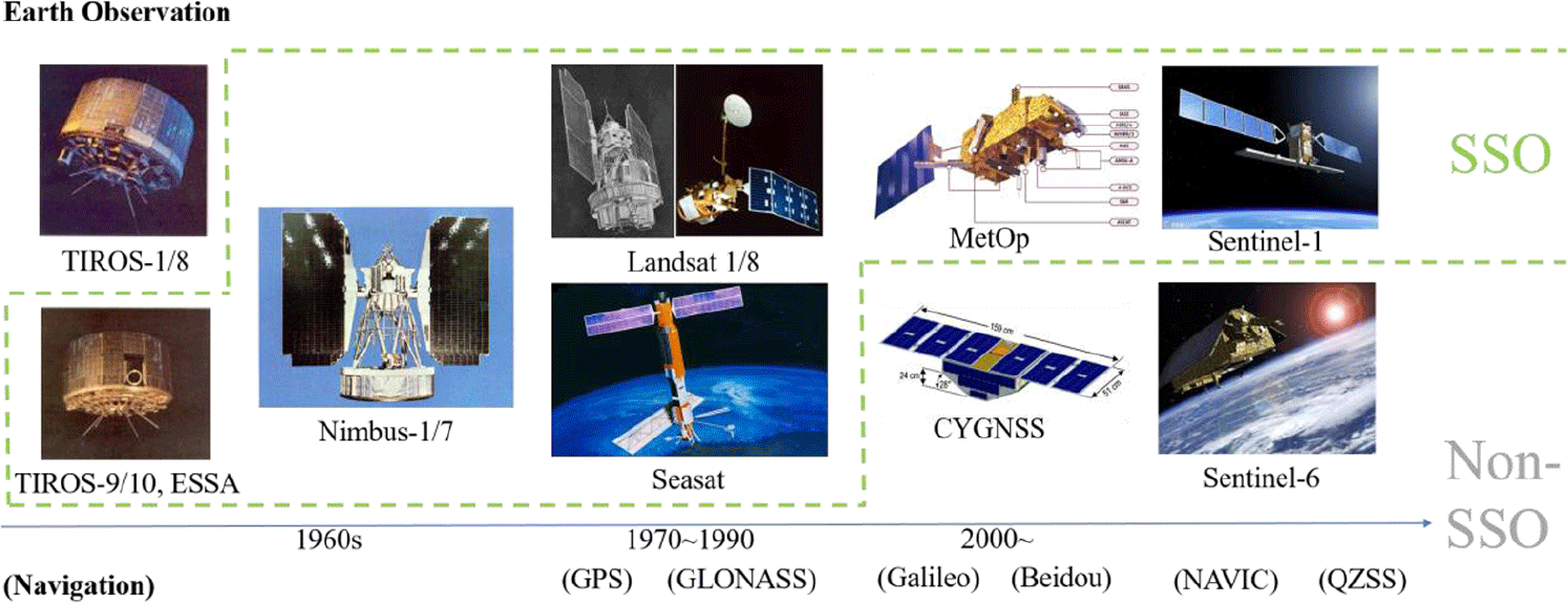
The development of meteorology and oceanography has been facilitated by remote sensing from space. The first-generation weather satellites used non-polar (i.e. low inclination) low-Earth orbits (LEOs) as illustrated by Television and Infrared Observation Satellites (TIROS, 1960). Since the second generation marked by the Nimbus series (1964), however, near-polar (i.e. high inclination) Sun-synchronous orbits (SSOs) have become the norm in Earth observation satellites as well as weather satellites(Reference Short, Lowman, Scott, Hobsh, Stoney, Rosalanka, Love, Robinson and Weissel1). The first Earth-studying satellite (Landsat-1, 1972) and the first ocean-research satellite (SeaSat, 1978) abided by this norm, followed by many others(Reference Irons, Taylor and Rocchio2). Remote-sensing satellites in SSOs cross a given horizontal latitude band at the same mean local time (MLT) throughout a year, providing uniform illumination conditions in visible or infrared wavelengths. Satellites in SSOs also usually have repeat ground tracks (RGTs), crossing a given vertical longitude line at the same MLT throughout a year. Having both SSOs and RGTs, therefore, would be ideal for observing stationary ground targets, predetermined by a set of latitude–longitude combinations at a designated time of a day on a regular basis.
On the other hand, radio-frequency measurements do not necessarily require SSOs. The Cyclone Global Navigation Satellite System (CYGNSS, 2016) measures GPS signals reflected from the oceans to measure wind speeds and does not use SSOs; eight microsatellites in the system orbit at an inclination of 35° and an altitude of 500km.(Reference Ruf, Atlas, Chang, Clarizia, Garrison, Gleason, Katzberg, Jelenak, Johnson, Majumdar, O’brien, Posselt, Ridley, Rose and Zavorotny3) Another example, which did not utilise Sun-synchronism, dates back to the Constellation Observing System for Meteorology, Ionosphere, and Climate (COSMIC, 2006) with an inclination of 72° and an altitude of 500km.(Reference Bauer, Radnóti, Healy and Cadinali4) Other preceding radio occultation (RO) missions all used SSOs as witnessed in the three Meteorological Operational Satellite Program of Europe (MetOp) satellites and Challenging Minisatellite Payload (CHAMP)(Reference Reigber, Helm and Rother5,6) . As for larger satellites equipped with synthetic aperture radar (SAR), Sentinel-6 satellites mark a milestone transitioning from an SSO to a non-SSO. Launched in 2020 by the European Organisation for Metrological Satellites (EUMETSAT), Sentinel-6 satellites will not use SSOs for the first time in the Sentinel series; they will instead use non-SSOs at a 1,336km altitude and a 66° inclination where their radar altimeters will measure the height and other characteristics of the global ocean surface except polar circles(Reference Paek, Kim, Kronig and De Weck7). Until now, SAR missions as a whole have been relying upon SSOs as illustrated by TerraSAR-X (2007), Advanced Land Observing Satellite series (ALOS-1 in 2006 and ALOS-2 in 2014) and Envisat (2002) since the first deployment of SAR in orbit by SeaSat (1978)(8). Figure 1 summarises and categorises the above-mentioned Earth observation missions according to whether SSOs are used or not. The GPS signals have turned out to be useful for Earth remote sensing, and therefore other navigation systems are also listed in Fig. 1, including GLONASS (Russia), Galileo (Europe), NAVIC (India) and QZSS (Japan).
Earth observation missions and classification of their orbits(Reference Irons, Taylor and Rocchio2–8).

Since the 2010s, the notion of distributed satellite missions (DSM) has matured in terms of terminology and taxonomy as small satellite constellations become more common. These include(Reference Le Moigne, Adams and Nag9) Doves (2014, 400km, 52°); QB50 (2017, 320km, 79°); Optical Communications and Sensor Demonstration (OCSD, 2017, 550km, 34°); Cubesat Proximity Operations Demonstration (CPOD, 2019); COSMIC (2019, 500km, 72°); and Proba-3 (2021, 600 to 60,530km elliptical, 59°). In light of the ever-diversifying applications of space-borne remote sensing as well as increased options for the satellite design and launch, this paper proposes several non-conventional satellite orbits. They are ‘tweaked’ variants of conventional SSOs using RGTs in that either Sun-synchronism or ground track repeatability is no longer strictly imposed. Before making such variations, we first revisit the principles of SSOs, RGTs and their combinations in the remainder of Section 1. After revisiting these theories of traditional orbits, the RGT requirement and the SSO requirement are relaxed in Sections 2 and 3, respectively, to derive new types of orbits useful for Earth remote sensing. Section 4 introduces special uses of traditional or non-traditional orbits to enable new kinds of missions, such as space-based solar power and the Internet of Things (IoT) in space.
1.1 Sun-synchronous orbits
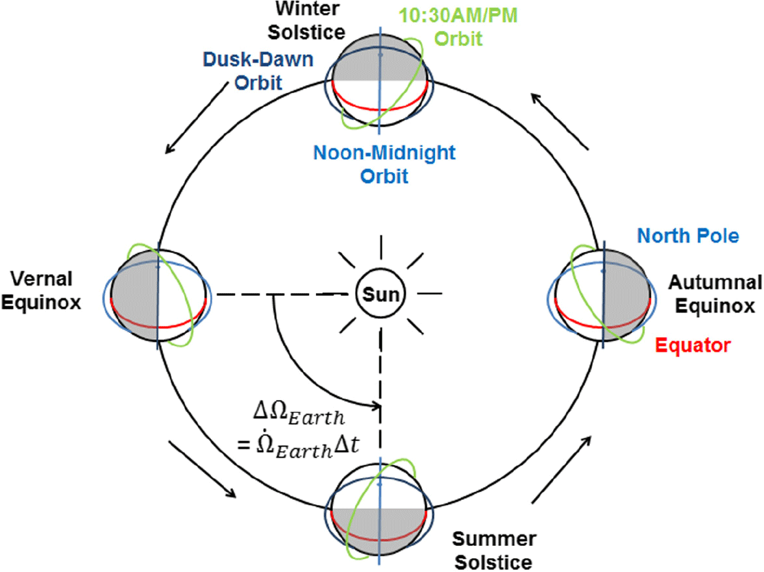
A SSO is a nearly polar orbit that regresses at a rate equal to the average rate of the Earth’s rotation around the Sun. In other words, the orientation of the orbit plane will remain nearly fixed with respect to the Sun throughout a year, and the satellite will pass the equator (and any location on the latitude band within satellite orbit inclination) at the same local mean solar time. If a satellite is in a dawn/dusk orbit (called a ‘twilight’ orbit until the 1970s), it crosses the equator around 15 times a day at 6:00 am/pm local time, as shown in Fig. 2. Because a dawn/dusk orbit allows local passages when day and night change, its satellite is said to be ‘riding the terminator’ whose constant Sun–Earth geometry is often useful for active instruments, passive instruments and solar observations. Examples of the last category of solar observatory spacecraft include Yohkoh (Solar-A), Hinode (Solar-B) and Transition Region and Coronal Explorer (TRACE). In lieu of riding the terminator, a Sun-synchronous satellite may be in a noon/midnight orbit or have any MLTs as scientific requirements may dictate(Reference Paek, Kronig, Ivanov and De Weck10,Reference Paek, Kim and De Weck11) . Figure 2 depicts a few SSOs that have different MLTs but all the same nodal regression rate, 360°/365.2422day = 0.9856°/day or 2 × 10⁻⁷rad/s(Reference Paek12).
Sun-synchronous orbits with different mean local times(Reference Paek12).
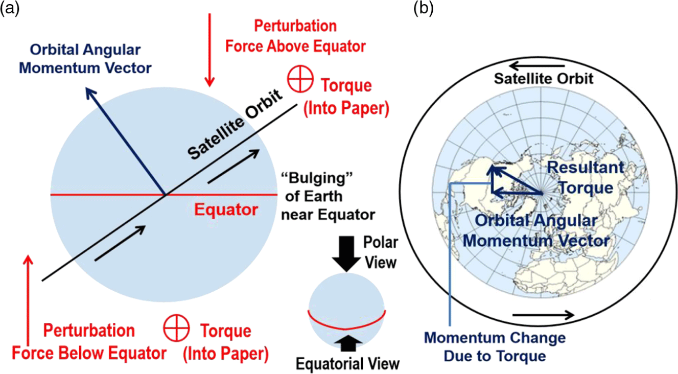
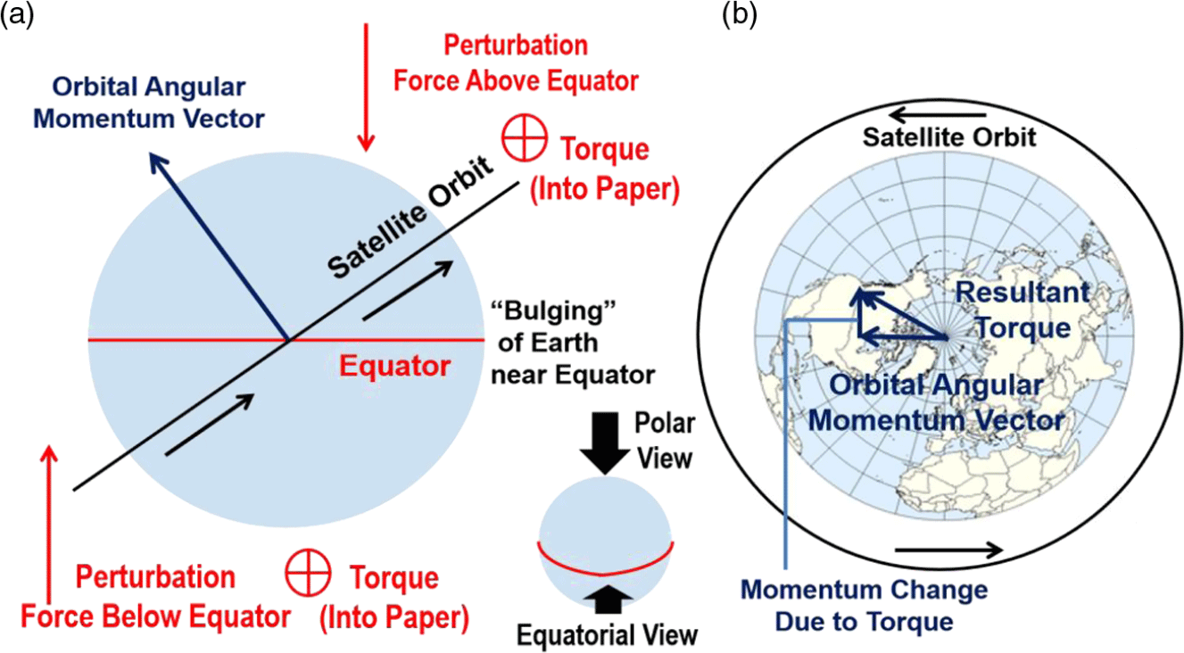
The regression of an SSO is caused by Earth’s oblateness or its equatorial bulge, whose mass exerts attractive forces on the orbiting satellite as illustrated in Fig. 3(a)(Reference Vallado13). The satellite trajectory is not deflected towards the equator, however, owing to its gyroscopic stiffness. The orbit inclination remains unchanged, while the orbit nodes regress instead as shown in Fig. 3(b), whose direction is westward (dΩ/dt < 0) for a prograde orbit (inclination < 90°) and an eastward (dΩ/dt > 0) or a retrograde orbit (inclination > 90°).
Nodal regression in Sun-synchronous orbits: (a) equatorial view and (b) polar view(Reference Vallado13).
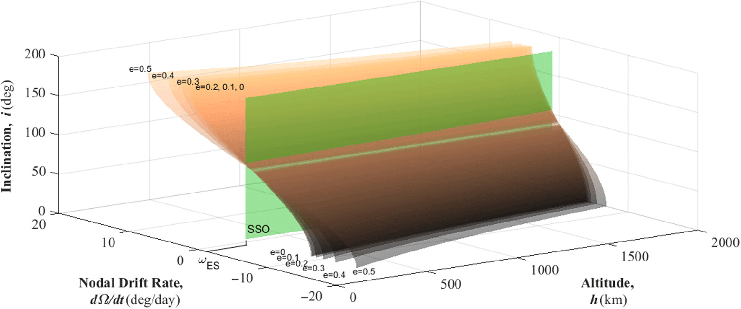
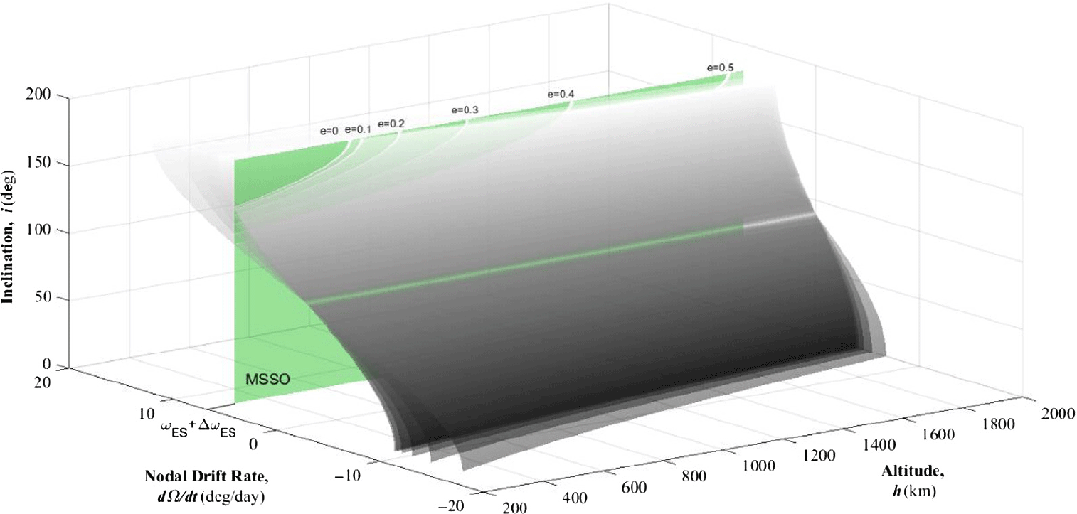
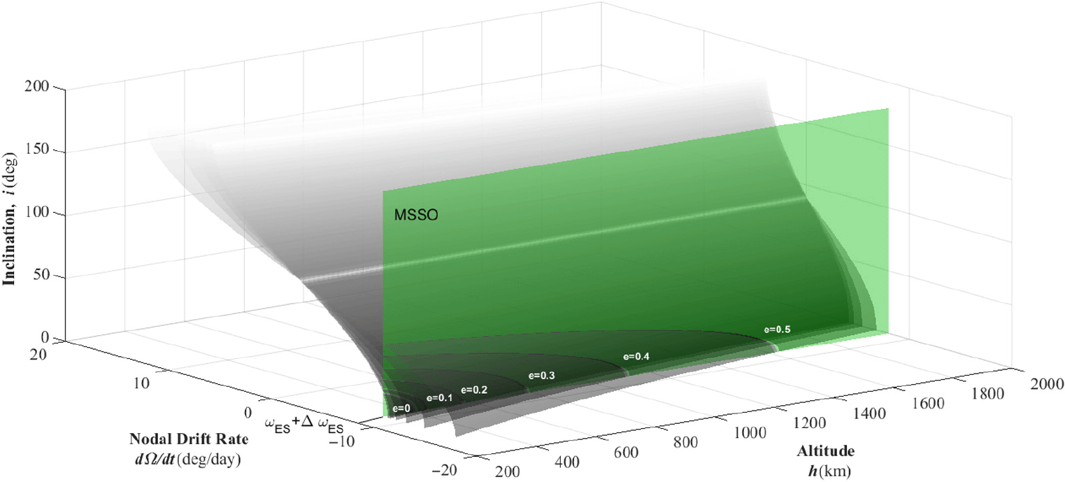
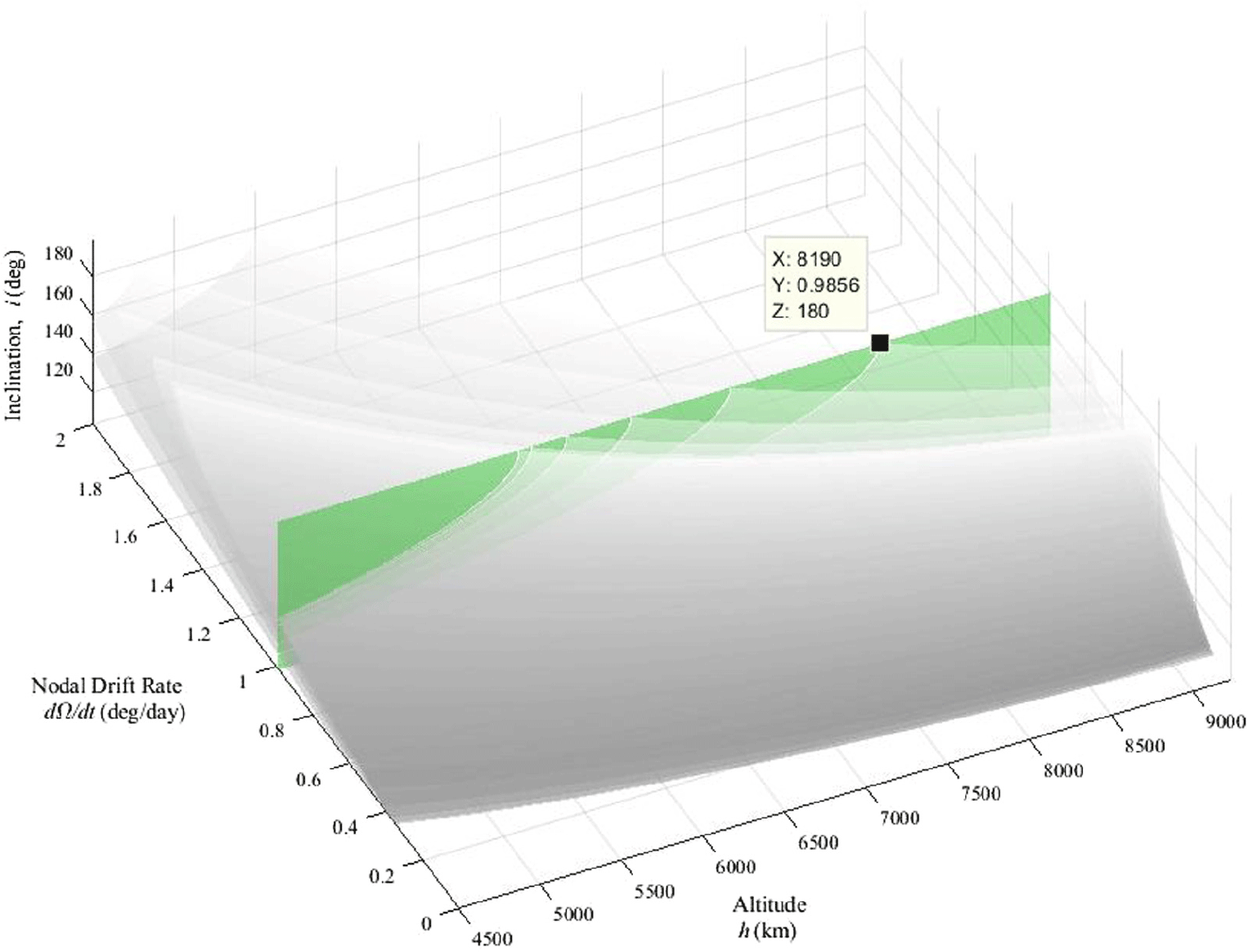
Relationship among altitude, nodal drift rate and inclination for different eccentricity values (curves) and the Sun-synchronous condition (vertical plane).

Equation (1) gives an orbital regression rate whose value must equal 0.9856°/day or 2 × 10⁻⁷rad/s in SSOs; dΩ/dt is the time derivative of longitude of ascending node Ω and is a function of semi-major axis (a), eccentricity (e), and inclination (i). Earth’s equatorial radius (R E = 6,378km) and standard gravitational parameter (μ E = 3.986 × 10⁵km3s–2) are used for Earth-centric orbits. A simplified geopotential model up to the second zonal term (J 2 = 1.08263 × 10⁻³) would suffice for the purpose and scope of this paper. Figure 4 depicts the relationship among dΩ/dt, semi-major axis and inclination for different eccentricities represented by curved surfaces. The vertical plane marks dΩ/dt = 0.9856°/day, whose intersection with curves represents all possible SSO solutions. This specific value of nodal regression (0.9856°/day) will be denoted as Ω ES henceforth throughout this paper.
 \begin{align}\dot \Omega = - \frac{{3R_E^2{J_2}\sqrt {{\mu _E}} }}{{2{a^{7/2}}{{\left( {1 - {e^2}} \right)}^2}}}cos\left( i \right)\end{align}
1.2 Repeat ground tracks
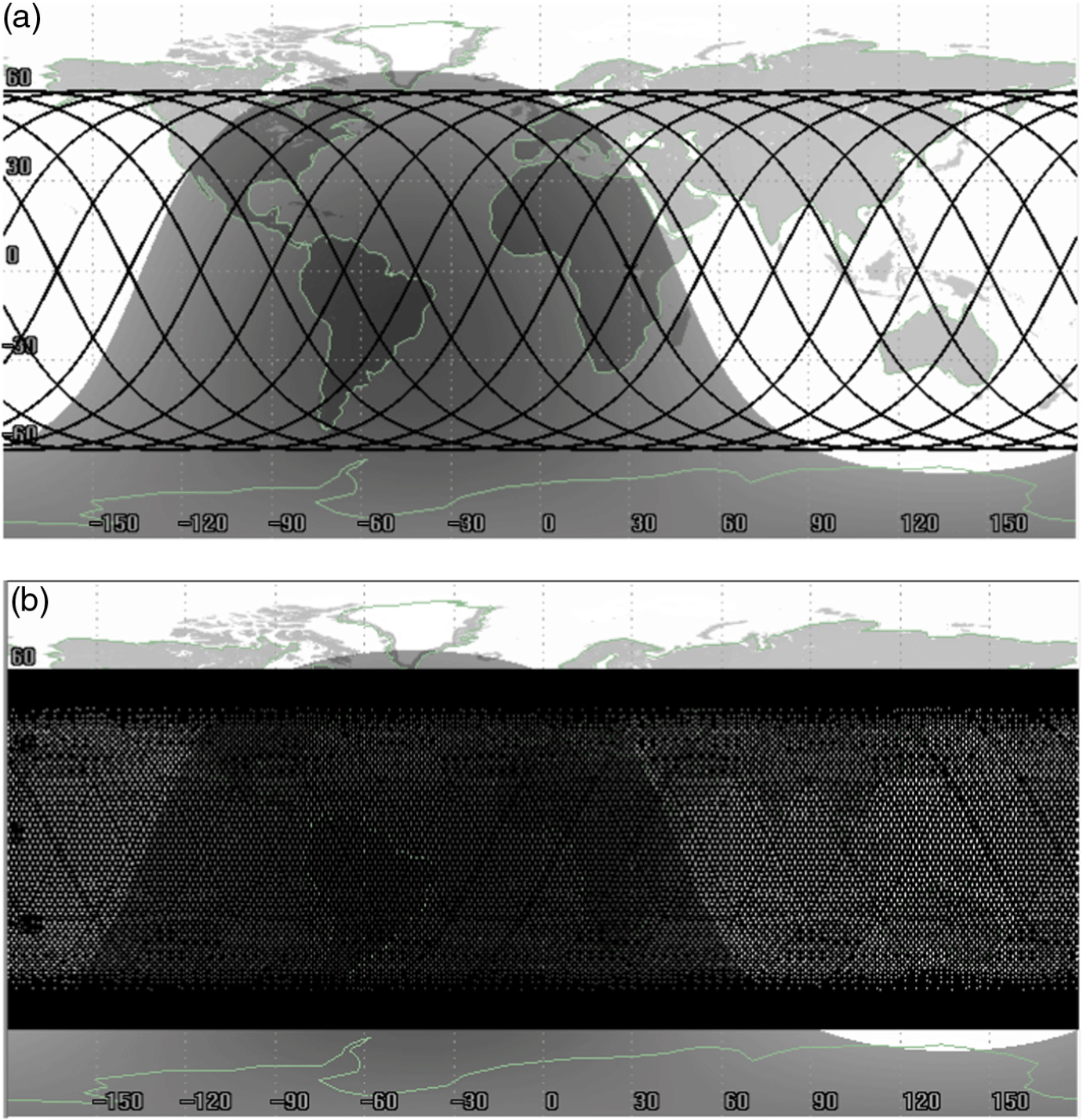
An orbit is said to have RGTs if a satellite’s ground track exactly repeats its pattern after a certain period of time, usually in days. Figure 5 illustrates two orbits with nearly identical altitudes (~500km)(Reference Paek, De Weck and Smith14); both orbits have 60° inclinations (not polar) and thus are not Sun-synchronous. A satellite in the first orbit leaves the exact same trace on the ground after 24 hours. The nodes of crossing, ascending from the lower left to the upper right, are separated by 24° because it orbits the Earth 15 times a day. The ground trace of the second orbit does not coincide with the starting point. The ground tracks will spread and cover the entire latitude, which is not conducive to the monitoring of specific targets due to much longer visit intervals than RGTs.
A non-Sun-synchronous orbit (inclination = 60°) with repeating ground tracks (a) and non-repeating ground tracks (b)(Reference Paek, De Weck and Smith14).

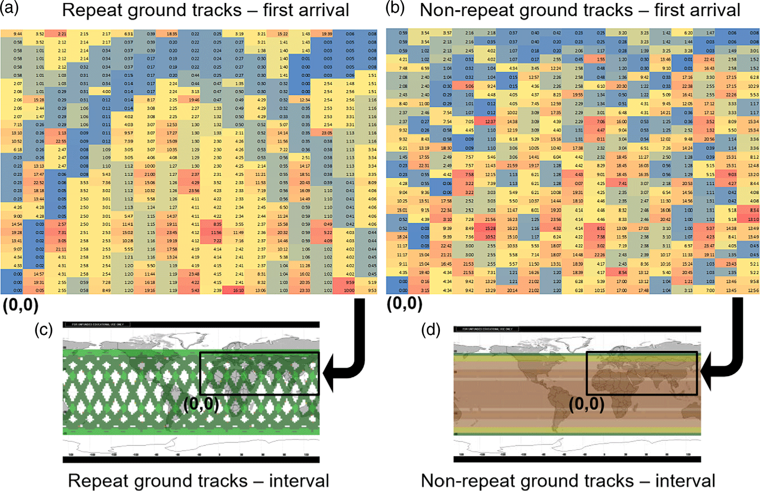
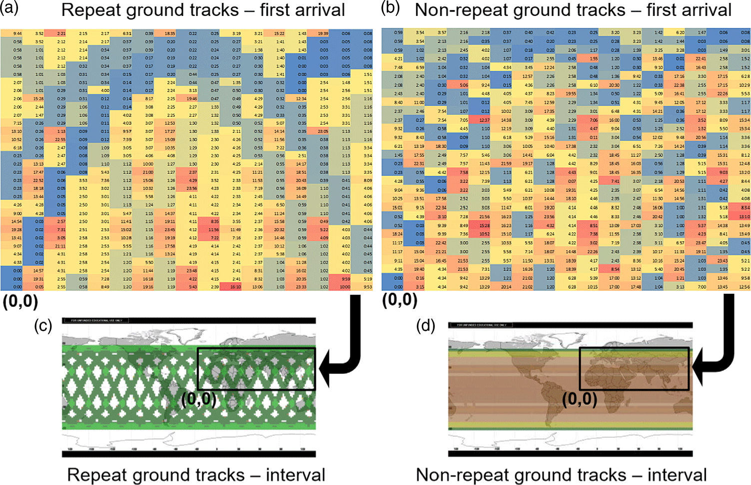
Figures 6(a) and (b) depict the time taken for a satellite initially at (longitude, latitude) = (0,0) to reach 10° × 1° grid points in the northern hemisphere for the first time. The averaged time of the first arrival for RGTs in Fig. 6(a) is more than twice that for non-RGTs in Fig. 6(b). This is because while RGTs provide a short visit interval of 1 day, as coloured in green in Fig. 6(c), they also leave inaccessible dead zones in between (no colour)(Reference Legge15). Non-RGTs, on the other hand, do not have dead zones and result in a lower averaged time of the first arrival; however, the revisit interval is higher than Fig. 6(b) as marked with yellow and red colours in Fig. 6(d).
Time of first arrival and visit interval of repeating ground track and non-repeating ground tracks(Reference Legge15).
The notation used in this paper is as follows: the satellite completes N S revolutions around the Earth after N D nodal days, with an Earth nodal period T N and a satellite orbital period T S defined as Equations (3) and (4), respectively(Reference Brucolleri16). The satellite period in Equation (3) contains the perturbed mean motion (dM/dt), which equals the unperturbed mean motion (n) plus the incremental term (Δn). The angular velocity of a satellite (n = 2π/T S = (μ E/a 3)1/2) around a perfectly spherical Earth is altered by Δn because of Earth’s oblateness. The perturbation in the argument of perigee (dω/dt) is added lastly to account for changing orbit directions, completing the effective angular velocity of a satellite. In a similar manner to the satellite period, the nodal period is affected by the Earth’s shape, but changing the node locations to cause three-dimensional wobbling in Fig. 2 rather than planar directional changes in the satellite period case. The dΩ/dt term from Equation (1) is subtracted from the Earth rotation rate ω E = 360°/day = 7.29 × 10⁻⁵rad/s in Equation (4) to yield the nodal period defined as the time between successive satellite passages measured at a given node.
 \begin{align}{N_S}{T_S} = {T_N}{N_D}\end{align}
 \begin{align}{T_S} = \frac{{2\pi }}{{\dot M + \dot \omega }} = \frac{{2\pi }}{{n + \Delta n + \dot \omega }}\end{align}
 \begin{align}{T_N} = \frac{{2\pi }}{{{\omega _E} - \dot \Omega }}\;\;\end{align}
Rearranging Equations (2), (3) and (4) gives a definition of the repeat ratio (τ) shown in Equation (5). In the definition used in this paper, the repeat ratio is always greater than 1 for orbits whose altitudes are smaller than that of a geostationary orbit (i.e. subsynchronous orbits). The expressions for Δn and are provided in Equations (6) and (7), respectively.
 \begin{align}\tau = \frac{{{N_S}}}{{{N_D}}} = \frac{{{T_N}}}{{{T_S}}} = \frac{{2\pi /\left( {{\omega _E} - \dot \Omega } \right)}}{{2\pi /\left( {\dot M + \dot \omega } \right)}} = \frac{{n + \Delta n + \dot \omega }}{{{\omega _E} - \dot \Omega }}\end{align}
 \begin{align}\Delta n = \frac{{3R_{\rm{E}}^2{J_2}\sqrt {{\mu _E}} }}{{4{a^{7/2}}{{\left( {1 - {e^2}} \right)}^{3/2}}}}\left( {2 - 3{{\sin }^2}i} \right)\end{align}
 \begin{align}\dot \omega = \frac{{3R_{\rm{E}}^2{J_2}\sqrt {{\mu _E}} }}{{4{a^{7/2}}{{\left( {1 - {e^2}} \right)}^2}}}\left( {4 - 5\,{{\sin }^2}\,i} \right){\rm{\;}}\end{align}
1.3 Sun-synchronous orbits with repeat ground tracks (SSRGT)
Having both SSO and RGT features gives many advantages in remote sensing, as explained in this paper’s Introduction, and is therefore the current norm for Earth observation satellites. Mathematically, the two features are achieved by setting dΩ/dt = ω ES = 0.9856°/day for all terms in Equation (5). Rearrangement of the substituted terms yields Equation (8), which is solved for the semi-major axis (a). To apply the Newton–Raphson method, Equation (8) is differentiated with respect to the semi-major axis as expressed in Equation (9). A recursive formula in Equation (10) is then reiterated until the solution converges.
 \begin{align} f(a) =\, & \sqrt {\frac{{{\mu _E}}}{{{a^3}}}} + \frac{3}{4}\frac{{{J_2}R_E^2\sqrt {{\mu _E}} }}{{{a^{\frac{7}{2}}}{{\left( {1 - {e^2}} \right)}^{\frac{3}{2}}}}}\left( {\frac{4}{3}\frac{{{a^7}\omega _{ES}^2{{\left( {1 - {e^2}} \right)}^4}}}{{J_2^2R_E^4{\mu _E}}} - 1} \right)\nonumber\\[10pt] & + \frac{3}{4}\frac{{{J_2}R_E^2\sqrt {{\mu _E}} }}{{2{a^{\frac{7}{2}}}{{\left( {1 - {e^2}} \right)}^2}}}\left( {\frac{{20}}{9}\frac{{{a^7}\omega _{ES}^2{{\left( {1 - {e^2}} \right)}^4}}}{{J_2^2R_E^4{\mu _E}}} - 1} \right)\end{align}
 \begin{align} f'\left( a \right) = & - \frac{3}{2}\sqrt {\frac{{{\mu _E}}}{{{a^5}}}} - \frac{{21}}{8}\frac{{{J_2}R_E^2\sqrt {{\mu _E}} }}{{{a^{\frac{9}{2}}}{{\left( {1 - {e^2}} \right)}^{\frac{3}{2}}}}}\left( {\frac{4}{3}\frac{{{a^7}\omega _{ES}^2{{\left( {1 - {e^2}} \right)}^4}}}{{J_2^2R_E^4{\mu _E}}} - 1} \right)\nonumber\\[10pt]
& - \frac{{21}}{8}\frac{{{J_2}R_E^2\sqrt {{\mu _E}} }}{{{a^{\frac{9}{2}}}{{\left( {1 - {e^2}} \right)}^{\frac{3}{2}}}}}\left( {\frac{{20}}{9}\frac{{{a^7}\omega _{ES}^2{{\left( {1 - {e^2}} \right)}^4}}}{{J_2^2R_E^4{\mu _E}}} - 1} \right)\nonumber\\[10pt]
& + \frac{{7{{\left( {1 - {e^2}} \right)}^{\frac{5}{2}}}\omega _{ES}^2}}{{{J_2}R_E^2{\mu _E}}}\sqrt {\frac{{{a^5}}}{{{\mu _E}}}} + \frac{{35{{\left( {1 - {e^2}} \right)}^2}\omega _{ES}^2}}{{3{{\kern1pt}J_2}R_E^2{\mu _E}}}\sqrt {\frac{{{a^5}}}{{{\mu _E}}}}
\end{align}
 \begin{align}{h_{n + 1}} = {h_n} - \frac{{f\left( {{h_n}} \right)}}{{f'\left( {{h_n}} \right)}}\end{align}
As will be shown later, the value of eccentricity does not affect the converged semi-major axis and inclination in SSRGTs. And for simplicity, circular orbits will be considered throughout this paper. Substitution of e = 0 into Equations (8) and (9) leads to Equations (11) and (12), respectively. Note also that semi-major axis (a) has been replaced by the sum of the Earth’s radius ( ${R_E}$) and height (h) to calculate altitude directly. An initial guess for the numerical method in Equation (10) may employ Equation (13), which would be the RGT orbit altitude if Earth were perfectly spherical(Reference Brucolleri16).
 \begin{align}f\left( h \right) = \sqrt {\frac{{{\mu _E}}}{{{{\left( {{R_E} + h} \right)}^3}}}} + \frac{{{J_2}R_E^2\sqrt {{\mu _E}} }}{{{{\left( {{R_E} + h} \right)}^{7/2}}}}\left( {\frac{8}{3}\frac{{{{\left( {{R_E} + h} \right)}^7}\omega _{ES}^2}}{{J_2^2R_E^4{\mu _E}}} + \frac{3}{2}} \right) + \left( {{\omega _{ES}} - {\omega _E}} \right)\tau \end{align}
 \begin{align}f{\rm{'}}\left( h \right) = \frac{{ - 18{{\kern1pt}J_2}R_E^2{\mu _E}{{\left( {{R_E} + h} \right)}^2} + 112{{\left( {{R_E} + h} \right)}^7}\omega _{ES}^2 + 63{\kern1pt}J_2^2R_E^4{\mu _E}}}{{12{{\kern1pt}J_2}R_E^2\sqrt {{\mu _E}} {{\left( {{R_E} + h} \right)}^{9/2}}}}\end{align}
 \begin{align}{h_0} = \sqrt[3]{{\frac{{{\mu _E}}}{{{\tau ^2}\omega _E^2}}}} - {R_E}\end{align}
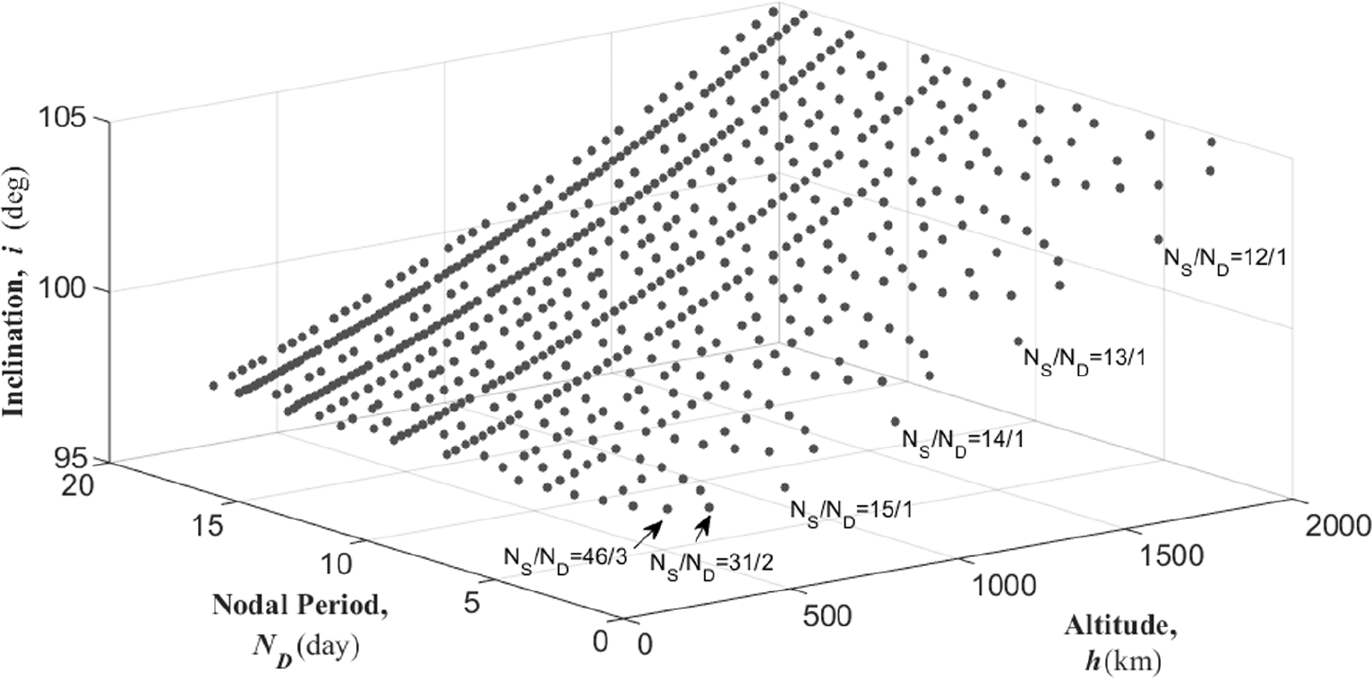
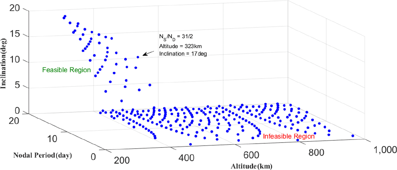
The relationship among altitude, inclination and RGT ratio (N S and N D) is depicted in Fig. 7; two (altitude and inclination) out of the three axes are identical to those in Fig. 4, and the nodal drift rate in Fig. 4 is now replaced with the nodal period in Fig. 7 because we are fixing the nodal drift rate to ω ES. One of the intersecting lines in Fig. 4, pointing upwards as altitude increases, now forms a curved surface in Fig. 7 via translation motion. The intersecting lines in Fig. 4 are almost identical for all values of eccentricities where increasing eccentricity from 0 to 0.5 for a τ = 15/1 orbit will change its altitude of 720km by less than 3km. Because most of the eccentric orbits will have perigees too close above (or even beneath) the Earth, only a circular orbit (zero eccentricity) is delineated in Fig. 7 and will be considered throughout the rest of this paper.
Relationship among altitude, nodal period and inclination for different satellite periods for Sun-synchronous orbits with repeating ground tracks (SSRGTs).

2.0 CLASS 1 VARIANTS: ORBITS WITH SUN-SYNCHRONISM
Section 1 provided a theoretical background for SSOs with RGTs (SSRGT). The first variant type relieves each condition to generate SSOs with drift ground tracks (SSDGT) and multi-SSOs with RGTs (MSSRGT).
2.1 Sun-synchronous orbit with drift ground tracks (SSDGT)
The first variation we can apply on SSRGTs is to allow the migration of ground tracks in a controlled way at a predefined speed. Such characteristics could be useful for tracking mobile targets when dynamic scheduling of sensor pointing may be more challenging than static targets(Reference Nag, Li and Merrick17). In an SSRGT orbit with an RGT ratio of 15 and an altitude of 561km, a satellite returns to the starting location every day after 15 revolutions. If the altitude is decreased to 500km, the satellite will arrive 500km east to the starting point, corresponding to a drift speed of 20km/h at the equator. The drifting of ground tracks comes from the difference in orbital periods between an RGT orbit and a DGT orbit. If the semi-major axis (altitude) of the non-RGT orbit deviates from that of a RGT orbit by Δa, its orbital period difference is given by Equation (14), corresponding to ground displacement at the equator in Equation (15).
 \begin{align}\Delta T = 2\pi \left( {\sqrt {\frac{{{{\left( {a + \Delta a} \right)}^3}}}{{{\mu _E}}}} - \sqrt {\frac{{{a^3}}}{{{\mu _E}}}} } \right)\end{align}
 \begin{align}\Delta d = \left( {{\omega _E} - \dot \Omega } \right){R_E}\Delta T\end{align}
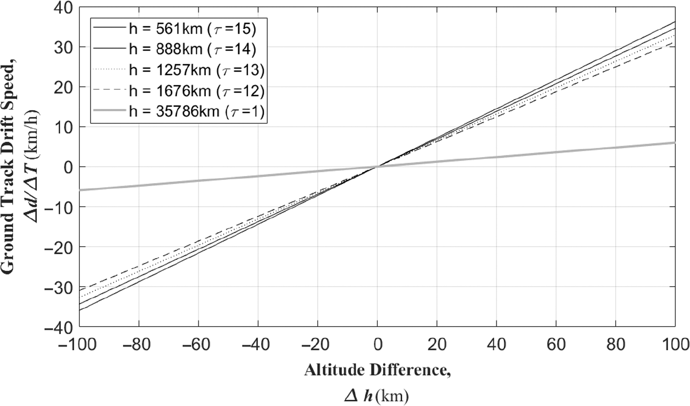
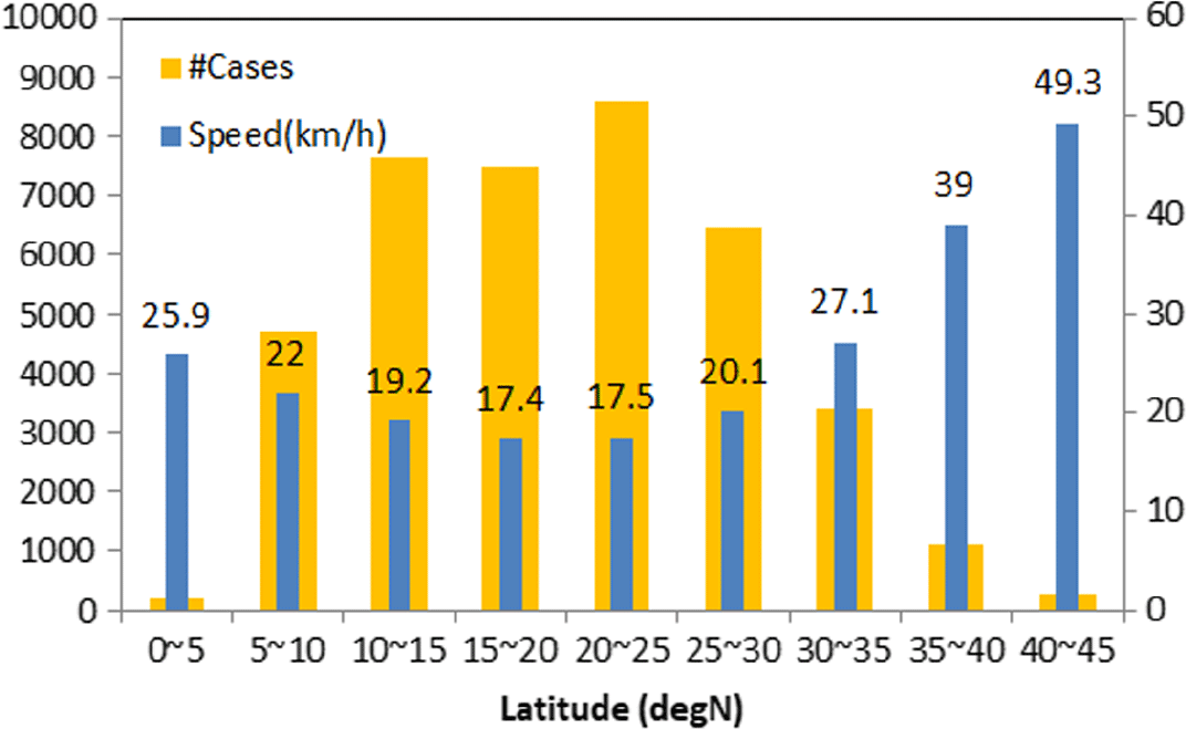
If Δa > 0, the DGT orbital period increases (ΔT > 0); its ground tracks drift eastward as indicated from Δd > 0. If Δa < 0, the DGT with a shorter period will lead the counterpart RGT (ΔT < 0), therefore drifting westward with Δd < 0. Consideration of two extreme cases, a LEO satellite and a geostationary satellite, may help visualise and understand this. While a LEO satellite moves from lower left to upper right, its traces will move westward crossing the equator every 90 minutes; the sub-satellite point of a geostationary orbit will be stationary due to its one-day period. Figure 8 shows the almost linear trend between Δd/ΔT and Δa for different altitudes. The drift velocity has very similar slopes in LEOs where the ground track speeds increase by approximately 0.3km/h as the altitude increases by 1km. This characteristic may be useful in tracking mobile targets because the resolution of satellite imagery is maximised when the distance between a satellite and a target is minimised. For instance, these kinds of orbits can be used for tracking tropical storms such as hurricanes. Figure 9 summarises the ground speed statistics of Atlantic hurricanes, excerpted from the National Hurricane Center’s North Atlantic hurricane database(Reference Dorst18). The data spans a time period between 1851 and 2014, in which over 70% of the cases the ground speed was around 20km/h between 10°N and 30°N latitudes. This speed corresponds to the common altitude offset of 50km in semi-major axis (altitude) in Fig. 8. Also note that the ground track speed is slowed down in higher altitudes such as the geosynchronous orbit with the RGT ratio of 1.
Ground track speeds of drift orbits offset from baseline orbits.

Active orbit manoeuvre for mobile target tracking(Reference Paek and De Weck19)

Distribution of hurricane speeds in the northern Atlantic Ocean between 1851 and 2014(Reference Dorst18).

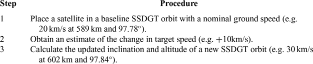
Outside the 10°N and 30°N latitude band, the drift speed increases over 25km/h. Making use of weather databases, a reduced-order model solved by onboard computing or a full-order model solved by ground computing power, a tropical storm’s path may be predicted and the satellite may change its path using procedures described in Table 1(Reference Paek and De Weck19). The required ΔV is usually less than 10m/s, which is added to the baseline Δv budget of a non-drifting orbit. For a five-year mission, the Δv required for air-drag corrections and de-orbiting of a stationary orbit is minimised around 150m/s at 550km, below and above which are mostly governed by fuel consumption due to atmospheric drags and de-commissioning, respectively(Reference Legge15). An additional 10m/s per year would be required to correct orbital drifts owing to non-spherical effects of the Earth. A total sum of everything, a few hundreds of m/s, can be covered sufficiently with present technologies for chemical propulsion. Some electric propulsion methods (arcjet or resistojet), if combined with chemical methods that utilise the same propellants, could balance the fuel economy and response time. Excessive fuel consumption for manoeuvres may also be avoided with pre-scheduled satellite pointing or deploying multiple satellites to match different drift speeds. The DGTs might also be useful for the real-time monitoring of ships and trash in the ocean(Reference Richter, Eyring, Burrows, Bovensmann, Lauer, Sierk and Crutzen20,Reference Lebreton, Slat, Ferrari, Sainte-Rose, Aitken, Marthouse, Hajbane, Cunsolo, Schwarz, Levivier, Noble, Debeljak, Maral, Schoeneich-Argent, Brambini and Reisser21) .
2.2 Multi-sun-synchronous orbit with repeat ground tracks (MSSRGT)
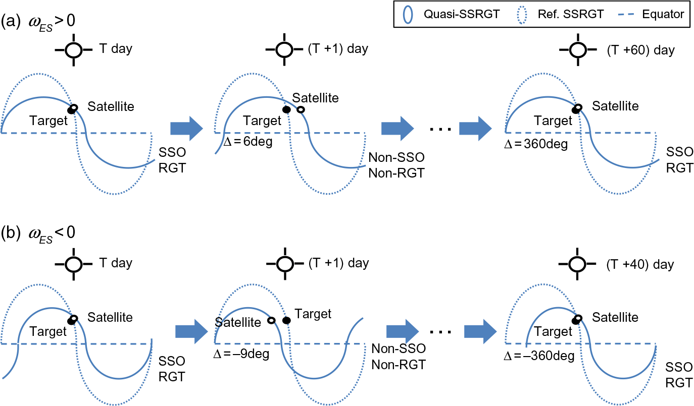
Another variant of SSRGTs retains Sun-synchronism but loosens it by not imposing the requirement every day. The resulting concept of so called ‘multi-Sun-synchronous’ orbits has already been proposed in earlier literature, but their RGTs were not taken into account, lacking practical considerations in remote sensing applications(Reference Mortari, Matthew, Wilkins and Bruccoleri22). This section builds on our discussions made in Section 1.1 to provide broader perspective in the orbital elements domain because it was also lacking in earlier literature that focused on few orbit designs(Reference Ulivieri and Anselmo23). Multi-SSOs have a nodal regression rate of dΩ/dt = ω ES + Δω ES, where Δω ES is a correction factor. Use of this ‘boost’ factor by substituting ω ES with ω ES + Δω ES in Equation (3) has an equivalent effect of sliding the vertical plane in Fig. 4 to the left (Δω ES > 0) or right (Δω ES < 0). Possible solutions on the intersecting line may be expanded in a similar manner to Fig. 7 such that MSSRGTs may be identified. The multi-SSRGTs will provide identical solar angles every |360/Δω ES| days, as illustrated in Fig. 10.
Comparison of SSO and MSSRGT orbits with (a) positive Δω ES and (b) negative Δω ES.

Relationship among altitude, nodal drift rate and inclination for different eccentricity values (curves) and the multi-Sun-synchronous condition with Δω ES = 6°/day (vertical plane).

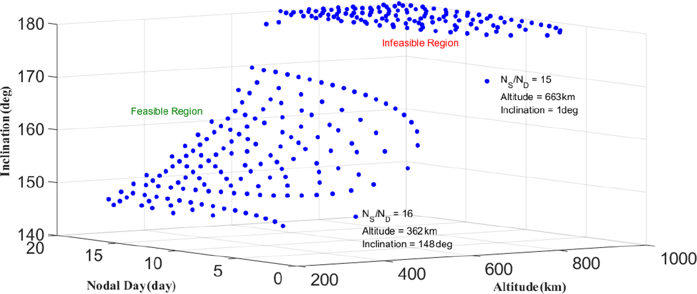
For a Δω ES value of 6°/day in Fig. 11, the vertical plane in Fig. 4 is shifted to the left whose intersection becomes considerably shorter than the baseline case of Δω ES = 0. Thus, a circular MSSRGT orbit (zero eccentricity) can have a maximum altitude less than 700km. The intersection and the maximum altitude are also illustrated in Fig. 11 for different nodal periods. Beyond the intersection is the infeasible region where inclination exceeds 180°; the maximum altitude of 663km corresponds to a 172° inclination.
Relationship among altitude, nodal period and inclination for different satellite periods for MSSRGTs where Δω ES = 6°/day.

The above plateaued shape is inverted for negative Δω ES values, as shown in Fig. 13 with Δω ES = −9°/day. Sun-synchronous conditions are achieved at an interval of 40 days (360°/(9°/day)) and are applicable to equatorial orbits with inclinations as low as 17° in Fig. 14. The low frequency of SSO conditions may be compensated with satellite swarms distributed over multiple orbit planes.
Relationship among altitude, nodal drift rate and inclination for different eccentricity values (curves) and the multi-Sun-synchronous condition with Δω ES = −9°/day (vertical plane).

Orbit parameters of MSSRGT orbits and SSOs

Relationship among altitude, nodal period, and inclination for different satellite periods for MSSRGTs where Δω ES = −9°/day.

Table 2 compares the inclination of select MSSRGT orbits and that of SSRGT orbits with similar heights(Reference Paek, Kronig, Ivanov and De Weck10). Although the MSSRGT orbits achieve Sun-synchronism less frequently than SSRGT orbits, the former provides more coverage to near-equatorial regions due to lower inclinations than the latter. Figure 6(d) illustrates this phenomenon of increased coverage at zones whose latitudes are similar to the orbit inclination (green at top and bottom). In order to compare the coverage performance of two types of orbits, we should consider both the individual satellite design (e.g. sensor boresight angle) and the overall constellation geometry(Reference Paek, Kim and De Weck11).
2.3 Multi-sun-synchronous orbit with drift ground tracks (MSSDGT)
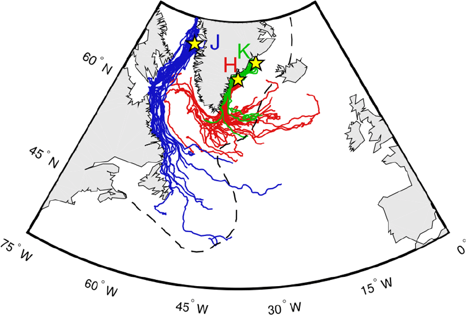
The last variation combines multi-Sun-synchronism and drift ground tracks leading to a category of MSSDGTs whose altitudes differ from MSSRGT by a certain amount to produce the desired ground track speeds. Because the time interval between observations is rather long, MSSDGTs would be suitable for slow-moving targets such as glaciers or icebergs that have been experiencing ever-growing impacts from climate changes. There is a long-standing rule of thumb that Arctic icebergs drift at 2% of the relative wind speed with respect to the ocean current (‘2% rule’). This iceberg speed is at least an order of magnitude slower than North Atlantic hurricanes considered in Section 2.1; it has also been shown that Antarctic icebergs have even slower drift velocities due to their plateaued shape and weak winds. Figure 15 presents simulated drift trajectories of Arctic icebergs released at three glacier outlets in Greenland(Reference Wagner, Dell and Eisenman24). The motion of icebergs follows the coastline and whose direction and speed may be used to determine the required DGT altitude offsets.
Simulated trajectories of icebergs released at different parts in Greenland: Kangerlussuaq (K), Helheim (H) and Jakobshavn (J)(Reference Mortari, Matthew, Wilkins and Bruccoleri22).

3.0 CLASS 2 VARIANTS: ORBITS WITH MOON-SYNCHRONISM
Besides the Sun, the Moon is another celestial body that exerts considerable gravitational forces on Earth, creating lunar tides. Bio-optical reflectance of coastal waters is characterised by local hydrographic features and phytoplankton composition that depend on lunar tides. It is also an active area of research because accelerating climate changes and increasing sea levels are causing impacts on estuaries and coastal regions whose vast scales could best be studied with satellite remote sensing(Reference Nag, Li and Merrick17,Reference Ulivieri and Anselmo23) . Tidal synchronous orbits (TSOs) are obtained by replacing the Earth’s spin rate ω E in Equation (5) with the Moon’s rotation rate around the Earth ω EM. The Moon’s revolution period (one tidal lunar day) is T L = 2π/ω EM = 24h 50m 8s, which is slightly longer than one Earth sidereal day equal to T D = 2π/ω E = 23h 56m 4s because the Moon orbits around Earth in the same direction as the Earth spins. Equation 16 also shows that the lunar repeat ratio τ L is defined using the lunar nodal period T L and the number of lunar revolutions N L.
 \begin{align}{\tau _L} = \frac{{{N_S}}}{{{N_L}}} = \frac{{{T_L}}}{{{T_S}}} = \frac{{2\pi /\left( {{\omega _{EM}} - \dot \Omega } \right)}}{{2\pi /\left( {\dot M + \dot \omega } \right)}} = \frac{{\dot M + \dot \omega }}{{{\omega _{EM}} - \dot \Omega }}\end{align}
Because the Moon’s rotation rate in this formulation instead of the Earth’s spin rate defining nodal days, a TSO cannot have RGTs by nature. Nonetheless, one can still define a metric on how close a TSO is to an SSRGT orbit or an SSO. The node of an SSRGT orbit or an SSO drifts by 2π radians per year, so the closer a TSO’s yearly nodal regression approaches to 2π via minimisation of Ω year = |2π - dΩ/dt × T year|, the more it is SSRGT-like. Suppose a TSO with N L = 57 and N S = 885, such that its satellite completes 885 orbits every 57 tidal cycles, the satellite will fly over a location with the same tidal conditions that geographically differ from the starting location. It is possible to make (1) the current TSO more SSRGT-like, or (2) synchronise it also with the Sun; the following subsections discuss the two orbit categories derived from these options.
3.1 SSRGT-like tidal synchronous orbit
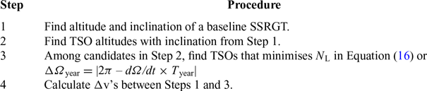
If the TSO uses an inclination of 97.6°, which is the same as SSRGT with a repeat ground track ratio τ = 15, it is an SSRGT-like TSO or quasi-SSRGT TSO. The TSO has an annual nodal drift of 355°/year, differing by only 5°/year compared to an SSO(Reference Lowe, Macdonald, Greenland and Mckee25). It is neither exactly an SSO nor an RGT orbit but is close to both if the ΔΩ year = 5°/year threshold is regarded ‘SSRGT-like’ enough. From the other perspective, this SSRGT orbit may be seen as TSO-like by commutative property. A simple algorithm is provided in Table 3, which identifies SSRGT-like TSOs near a baseline SSRGT(Reference Paek and De Weck19).
Search algorithm for SSGT-like TSOs

Δv (m/s) map of major SSRGTs and neighbouring TSOs(Reference Paek and De Weck19).

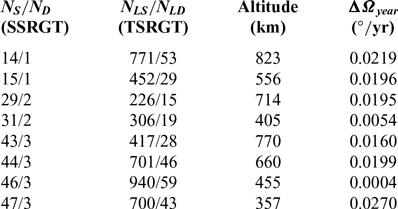
TSRGT orbits with minimum ΔΩ year

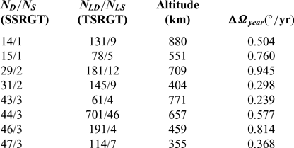
TSRGT orbits with minimum  $N_{\textrm{L}}$ and
 ${\bf{\Delta }}{{\bf{\Omega }}_{{\rm{year}}}} < (1^\circ {\rm{ }}/{\rm{yr}})$

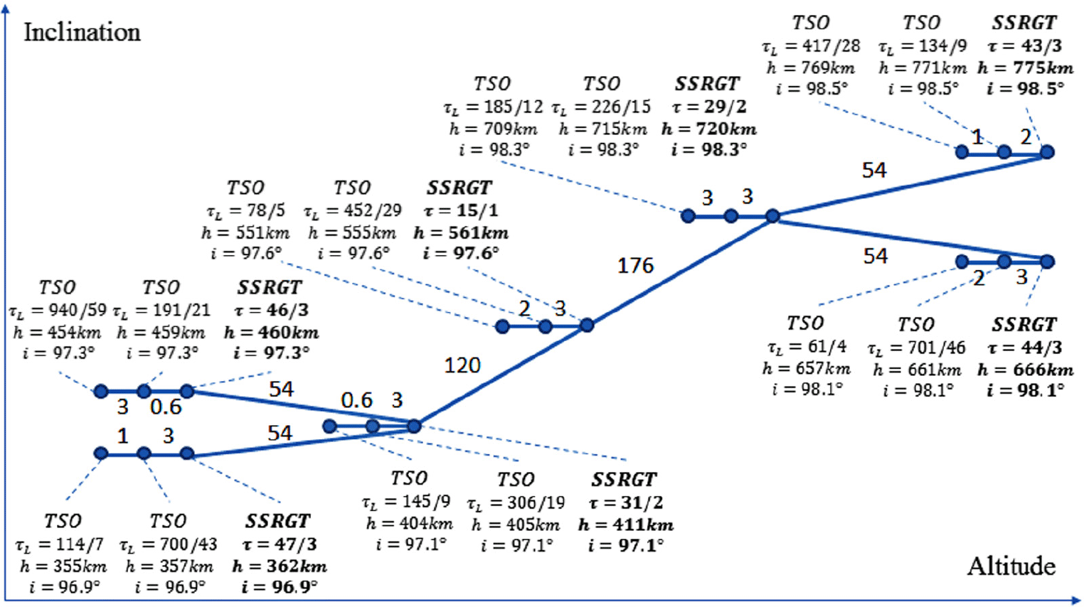
Applying these procedures to several SSRGTs reveals a Δv map similar to that for interplanetary transfers (lunar transfer orbit, LTO) or communications satellites (medium-Earth orbit, MEO) but in a much finer scale(Reference De Weck, Scialom and Siddiqi26). Figure 16 is a micro-scale Δv map for Earth-observation satellites(Reference Paek and De Weck19). The horizontal axis represents the orbit altitude, and the vertical axis corresponds to the orbit inclination (not to scale). For simplicity, only a few baseline SSRGT orbits in Fig. 7 were drawn, corresponding to the following number of satellite periods: 15 revolutions over 1 day; 29 and 31 revolutions over 2 days; 43, 44, 46, and 47 revolutions over 3 days. Two neighbouring TSO orbits were drawn for each SSRGT orbit: one that minimises ΔΩ year and the other that minimises the number of T L cycles while keeping ΔΩ year below 1°/year (more stringent than 5°/year requirement above). The first TSO option (minimising ΔΩ year) had a Right Ascension of the Ascending Node (RAAN) drift rate deviating from 360°/year by less than 0.05°/year, very close to the baseline SSRGT. Making deviation completely zero (TSSO) is not possible unless we (1) use indefinitely large N L and N S, as listed in Table 4, or (2) tilt the orbit inclination and cause departures from the baseline SSRGT (Table 5). The second option (minimising N L) results in orbits that have smaller lunar tidal days (denominator of τ L) than the first option. Keeping the number of repeat cycles low can bring back the same remote-sensing conditions more frequently; for example, a TSO with τ L = 78/5 is synchronised with 5 tidal lunar days and nearly (but not quite) 1 solar day; another TSO with τ L = 61/4 is synchronised with 4 tidal lunar days and nearly 3 solar days. Both options are only a few m/s away from the baseline SSRGT in Δv, as shown in Fig. 16, whose manoeuvres are achievable with current propulsion technology as well as ion propulsion(Reference Bourgoin, Meyer-Scott, Higgins, Helou, Erven, Hübel, Kumar, Hudson, D’souza, Girard, Laflamme and Jennewein27).
3.2 Tidal-sun-synchronous orbit
Returning to the example TSO with N L = 57 and N S = 885 assumed in Section 3.0, there is another possibility to proceed. If the TSO uses an inclination of 97.7°, instead of the original inclination of 97.6°, the annual RAAN drift becomes exactly 360°/year, achieving Sun-synchronism by abandoning ground track repetition. The ground tracks of this TSO are now far from SSRGTs, but it achieves synchronisation with the Moon and the Sun at the same time. This ‘Tidal-Sun-synchronous’ orbit (TSSO) incorporates lunar-solar dual-synchronism, which already exists in nature as spring tides and neap tides. A few non-remote-sensing applications of TSSOs are discussed in the next section. It should also be noted that multiple-synchronism can be incorporated to derive multiple-TSSOs (MTSSOs), MSSRGT-like TSOs, SSRGT-like multi-TSOs and so forth that are to be populated in the micro-Δv map above.
4.0 OTHER MISSIONS AND ORBIT VARIANTS
In addition to the aforementioned classes, orbits may be synchronised with other objects such as satellites orbiting Earth, which could facilitate the maintenance of constellations in particular. Also, the applications of orbit types discussed in this paper are not limited to Earth remote sensing. This section takes a look at future space missions where the new types of missions may be employed.
4.1 Use of tidal-sun-synchronous orbits in communications
The first application of TSSOs other than Earth observation purposes may be found in communications. In a future scenario of quantum communications, TSSOs provide uniform and controlled background noises from the Sun and the Moon. Low-Earth altitudes seem promising in the near term considering present technology readiness, and the quantum key distribution (QKD) link shall be operated at night-time to reduce noise levels(Reference Bourgoin, Meyer-Scott, Higgins, Helou, Erven, Hübel, Kumar, Hudson, D’souza, Girard, Laflamme and Jennewein27). The satellites in the orbit may also be equipped with scientific experiment platforms to conduct long-distance Bell tests and quantum teleportation (entanglement) experiments.
4.2 Use of sun-synchronous orbits with repeating ground tracks in non-remote-sensing applications and their physical limits
The use of SSRGTs could be useful for transmitting a large amount of data or power. The concept of satellite solar power stations (SSPS) has been studied for a wide range of orbits from LEO to Molniya orbit and geostationary Earth orbit (GEO)(Reference Chaudhary and Vishvakarma28). Although GEO would provide constant conditions for both power generation and rectenna orientation, it is already heavily crowded with communications satellites. Besides, on-orbit technology demonstration is more likely to begin with lower-altitudes such as LEO and MEO owing to technical and logistical issues. The SSRGTs would be the second-best choice because they provide periodic uniform conditions for power generation and transmission. For similar reasons, deep space communications to support manned spaceflights and space stations may utilise SSRGTs or TSSOs (lunar outposts); the Tracking and Data Relay Satellite System (TDRSS) is currently being used to this by NASA, but the limited orbit slots in GEO and the lack of data-handling capacity may become an issue at the advent of burgeoning space exploration backed by civilian sectors. One should note, however, that Sun-synchronism is attainable up to a certain altitude only; an orbit cannot be Sun-synchronous beyond this ‘ceiling’ whichever combination of orbital elements (altitude, eccentricity, inclination) may be used. Figure 17 extends Fig. 11 to MEOs for different eccentricity values; the ceiling altitude for a circular SSO is approximately 6,000km and can be increased to 8,200km for e = 0.5 with a perigee height of approximately 900km. Although these elliptical orbits are all geometrically feasible with a perigee height of 2,900km, its perigee will drift because its inclination is not at a critical angle. One may follow the intersection line for a given eccentricity and then identify the altitude where inclination becomes 116° (critical).
Theoretical maximum altitudes for SSOs with different eccentricity values: 6,050 km (e = 0.1); 6,270 km (e = 0.2); 6,660 km (e = 0.3); 7,260 km (e = 0.4); 8,170 km (e = 0.5) from the leftmost intersection to the rightmost. For each eccentricity value, SSOs below the corresponding limits will have non-equatorial inclinations (i ≠ 180°).

4.3 Use of non-sun-synchronous orbits in remote-sensing applications
As mentioned in the Introduction, satellites with SAR or RO instruments do not necessarily need SSOs because their spectrum ranges are independent of solar illumination in visible or infrared wavelengths. By taking advantage of the Earth’s rotation, non-SSOs will actually require less propellant to enter a non-SSO with prograde orbits, than an SSO with retrograde orbits. Only RGT conditions may be imposed on their orbit design to provide regular visits to both targets and ground stations. Instead of ground locations, tidal locations (TSO) or even regions in the Earth atmosphere such as a Van Allen radiation belt or the South Atlantic Anomaly could be synchronised with non-SSOs.
4.4 Drift orbits relative to satellite constellations
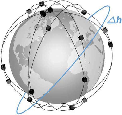
As several proposals are being made and implemented to provide global Internet coverage, management of massively deployed satellites is becoming increasingly important(8,Reference Le Moigne, Adams and Nag9) . OneWeb constellation will consist of 720 satellites weighing 150kg each, distributed over a total of 18 orbital planes(Reference Foreman, Siddiqi and De Weck29). The operational altitude is 1,200km high, and derelict satellites will be inserted into 1,100km × 240km disposal orbit for atmospheric re-entry upon the end of life. Telesat constellation consists of similar 1,248km-high inclined orbits but also features 1,000km polar orbits. For such massive constellations whose satellites carry minimal fuels, on-orbit servicing could be beneficial such as refuelling a satellite to extend life or deorbiting it to remove space debris. Offsets from the constellation’s baseline altitude can make this servicing satellite’s orbit plane to drift relative to the constellation, as illustrated in Fig. 18. Synchronising the RAAN drift rate of the servicing satellite and Walker spacing (inter-planar and intra-planar) of the constellation allows the servicing satellite and the serviced satellite to be in the same plane periodically, when the servicing satellite can raise or lower the altitude and rendezvous with the satellite to be serviced.
Servicing orbit drifting relative to a satellite constellation with altitude offset Δh.

5.0 CONCLUSION
This paper derived new types of Earth observation orbits based on traditional SSOs and RGTs. To obtain these orbit variants, constraints to attain desirable features were either partially relaxed or completely altered. In addition to the Sun, orbital synchronisation with the Moon and satellite constellations were also considered. Future work should consider design optimisation of satellites and constellations, as well as their mission planning, where the hereby proposed orbits and their enabling technologies (electric or hybrid propulsion) will be taken into account from long-term perspectives(Reference Paek, Kim and Payappan30). Continual refinement of the orbital taxonomy to equip ourselves with a ‘toolbox’ of orbits would also be conducive to future research activities in preparation of the new space age.
ACKNOWLEDGEMENTS
The authors would like to thank William Blackwell, Robert Legge and Sunghoon Baek for their support that inspired this work. Careful and constructive comments from anonymous reviewers are also much appreciated.