1 Introduction
In 1950, Morison et al. (Reference Morison, O’Brien, Johnson and Schaaf1950) proposed a decomposition of the hydrodynamic force on a monopile into drag and inertia components, each with an empirical coefficient to be determined from experiment. Lighthill (Reference Lighthill1986) discussed how the viscous drag force and the inviscid inertia force operate effectively independently, such that the total force can be decomposed into two distinct components. It is thus of interest to investigate this experimentally in the context of oscillatory flow past an array of small obstacles.
Current blockage in offshore engineering is defined as the local fluid velocity and associated hydrodynamic force (mainly drag) reduction on a structure due to the presence of such a structure as an obstacle array, which provides resistance to the incident wave and current flow. The phenomenon was first reported by Taylor (Reference Taylor1991) who derived an analytical blockage model accounting for flow reduction due to steady current flow (hence the term ‘current blockage’) as an improvement to the Morison equation (Morison et al. Reference Morison, O’Brien, Johnson and Schaaf1950) for multi-component space-frame structures. This work was further extended to regular waves with in-line current by Taylor, Santo & Choo (Reference Taylor, Santo and Choo2013) and Santo et al. (Reference Santo, Taylor, Williamson and Choo2014b ) who found that the additional hydrodynamic loading from waves contributes to additional force reduction, coining the term ‘wave–current blockage’. Their results have been validated extensively in experiments, ranging from small laboratory-scale tests involving perforated flat plates to large-scale tests using an offshore jacket model in a large towing tank, as well as numerical computational fluid dynamics (CFD) simulations using a porous block as a proxy for such structural models: see Santo et al. (Reference Santo, Taylor, Bai and Choo2014a ,Reference Santo, Taylor, Williamson and Choo b , Reference Santo, Taylor, Bai and Choo2015, Reference Santo, Stagonas, Buldakov and Taylor2017, Reference Santo, Taylor, Day, Nixon and Choo2018).
This paper extends previous research on wave–current blockage on statically responding (fixed bottom founded) space-frame offshore structures. Here we investigate the effects of blockage on dynamically responding structures and the validity of the relative-velocity formulation in the Morison equation. We speculate that the dynamic effect of structural motion, which is known to provide additional added mass, might also contribute to additional force reduction compared to wave–current blockage alone, providing the motivation for the present study. Examples of dynamically responding structures in offshore engineering include compliant towers, jack-ups and deep water jackets.
Previous studies have been conducted to investigate the relative velocity formulation in the Morison equation, primarily considering a single cylinder oscillated in otherwise still water: see for example Moe & Verley (Reference Moe and Verley1980), Williamson (Reference Williamson1985), Shafiee-Far, Massie & Vugts (Reference Shafiee-Far, Massie and Vugts1996), Burrows et al. (Reference Burrows, Tickell, Hames and Najafian1997) and Sumer & Fredsøe (Reference Sumer and Fredsøe2006). The relative-velocity formulation of the Morison equation includes interaction terms that involve both fluid and structural velocities and accelerations. Most of the work has assumed linear interaction between the ambient flow field and the structural motion, such that the flow kinematics can be superimposed in a similar way to waves and current. The aim of this paper is to examine the validity of the formulation when applied to multi-component space-frame structures where wave–current–structure blockage effects might be important.
We report a series of physical experiments, which are essentially a continuation of previous tests by Santo et al. (Reference Santo, Taylor, Williamson and Choo2014b ). Grids of perforated flat plates with square holes are moved in a towing tank through otherwise stationary water. Previously, two scales of forced oscillations were considered: steady flow and oscillatory (wave) motion. The present experiment adds a forced oscillatory structural motion, hence considering combined motions at three scales (in terms of both frequency and amplitude). Rectangular sharp-edged bars are used to force flow separation and thus to minimise Reynolds number effects. In the previous experiment, a systematic study was conducted by considering different porosity ratios and grid configurations (or number of plates). The present work considers three grids (perforated plates) with a specific porosity ratio (0.7) at each grid. An extension of the analytical wave–current blockage model is described, followed by detailed analysis and comparison with experimental data.
2 Experimental modelling
2.1 Experimental set-up
The experiments involve towing three grids comprising perforated flat plates in a large computer-controlled XY towing tank in Cornell University. The tank is
 ${\sim}6~\text{m}$
long, 1 m wide and 1 m deep. The water depth is 0.57 m. The tank is equipped with limit switches near both ends to prevent the carriage from moving too close to the end of the tank. The maximum distance of motion for the carriage is set at 4 m.
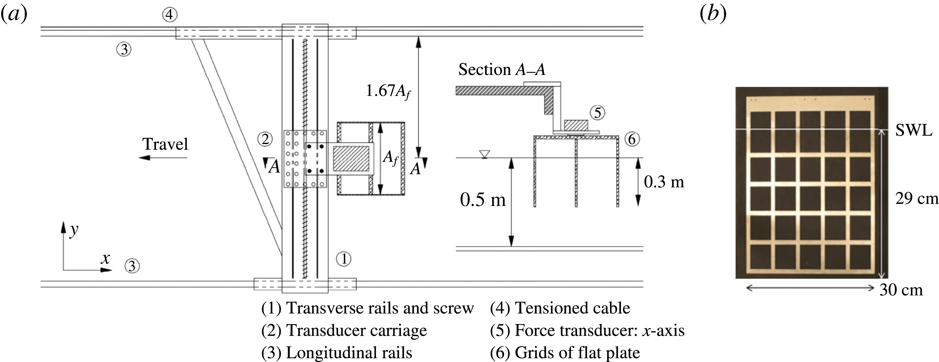
The set-up is illustrated in figure 1(a), a reproduction of figure 2 in Santo et al. (Reference Santo, Taylor, Williamson and Choo2014b
). Three grids of perforated thin plates are mounted below a force transducer, which is aligned in the
 $x$
-direction. The force transducer is then supported on a stiff plate and mounted on a carriage, which can be moved on rails by a motion-controlled tension cable in the
 $x$
-direction. The maximum speed of the carriage is limited to
 $20~\text{cm}~\text{s}^{-1}$
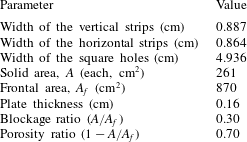
. Details of the grids are presented in figure 1(b) and table 1. When viewed from above (plan view), the cross-section of the grids is
 $0.3~\text{m}\times 0.3~\text{m}$
.
(a) Schematic diagram of the XY towing tank. (b) Elevation view of the grid.

Grid dimension details.

Motion of the grids was coordinated from a LabView interface on a PC through a programmable velocity–time history. The resulting load signals measured from a force transducer were recorded on the same interface. The sampling rate of the force data is 1000 Hz. The records were low-pass filtered at
 $12\times$
the frequency of the oscillatory wave motion, consistent with previous data analysis in Santo et al. (Reference Santo, Taylor, Williamson and Choo2014b
), with a smooth ramp down to zero of the frequency component at the top end of the band-pass range. All the filtering was done as post-processing in MATLAB. Additional treatment to the recorded force data due to a tank set-up error is described in appendix A.
2.2 Choice of parameters
The flow parameters are essentially the same as in Santo et al. (Reference Santo, Taylor, Williamson and Choo2014b
), and were chosen according to Keulegan–Carpenter number scaling on the entire grid (
 $KC=2\unicode[STIX]{x03C0}a/d$
, with
 $a$
being the amplitude of oscillation and
 $d$
being the strip width). The amplitude of oscillation and strip width were previously chosen to give a
 $KC$
value in the range of 10–40, as would occur for the main structural components of an offshore jacket platform in large waves. The second important scale is the width of the entire grid compared to the individual elements within the grid. This is approximately
 $40\times$
the size of the individual elements within the grid, a ratio appropriate for the width of an entire offshore structure compared to individual structural elements within the structure.
Due to the physical size limit of the towing tank, we simulate structural oscillation corresponding to realistic applications of the second mode of compliant towers (bending mode) and the first mode of jack-up legs (sway mode), whereby the structural oscillation frequency is larger than the wave oscillation frequency but the amplitude of the structural motion is smaller than the wave amplitude. Hence, we choose the structural to wave velocity ratio,
 $u_{s}/u_{w}=1/4-1/3$
, and structural to wave frequency ratio,
 $f_{s}/f_{w}=2$
, 2.5 and 3. While the steady motions are simply constant in time, the oscillatory motions are sinusoidal. Several motion combinations for a fixed ratio of
 $u_{w}/u_{s}$
and
 $f_{s}/f_{w}$
are possible by having the velocity peaks in phase at
 $t=0$
(label A), and the low and high frequency velocities out of phase by
 $\unicode[STIX]{x1D719}=\unicode[STIX]{x03C0}$
(label B) or phase-shifted by
 $\unicode[STIX]{x1D719}=\unicode[STIX]{x03C0}/2$
(label C), where
 $\unicode[STIX]{x1D719}$
is the phase shift. A waiting time of 20 min between each test was chosen to allow settling of the water in the tank.
This paper focuses on the range defined as
 $u_{c}/u_{w}=1/4-1/3$
in keeping with the analytical model derived for asymptotic conditions which are most important for extreme forces on offshore structures. For this asymptotic range, the resultant
 $KC$
value falls in the range of 40–70, which is justified considering the diameter of the main legs of a compliant tower is likely to be smaller than that of an equivalent jacket on the same water depth. Guided by the actual applications in the offshore industry, the amplitude of the wave oscillation should not be too large such that the wave velocity will become blocked by the obstacle array. Even for extreme waves incident on a full-scale offshore platform, the wave height would generally be smaller than the frontal width (or downstream length) of the whole space frame so the wave kinematics would only be weakly blocked if at all.
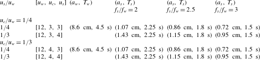
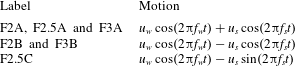
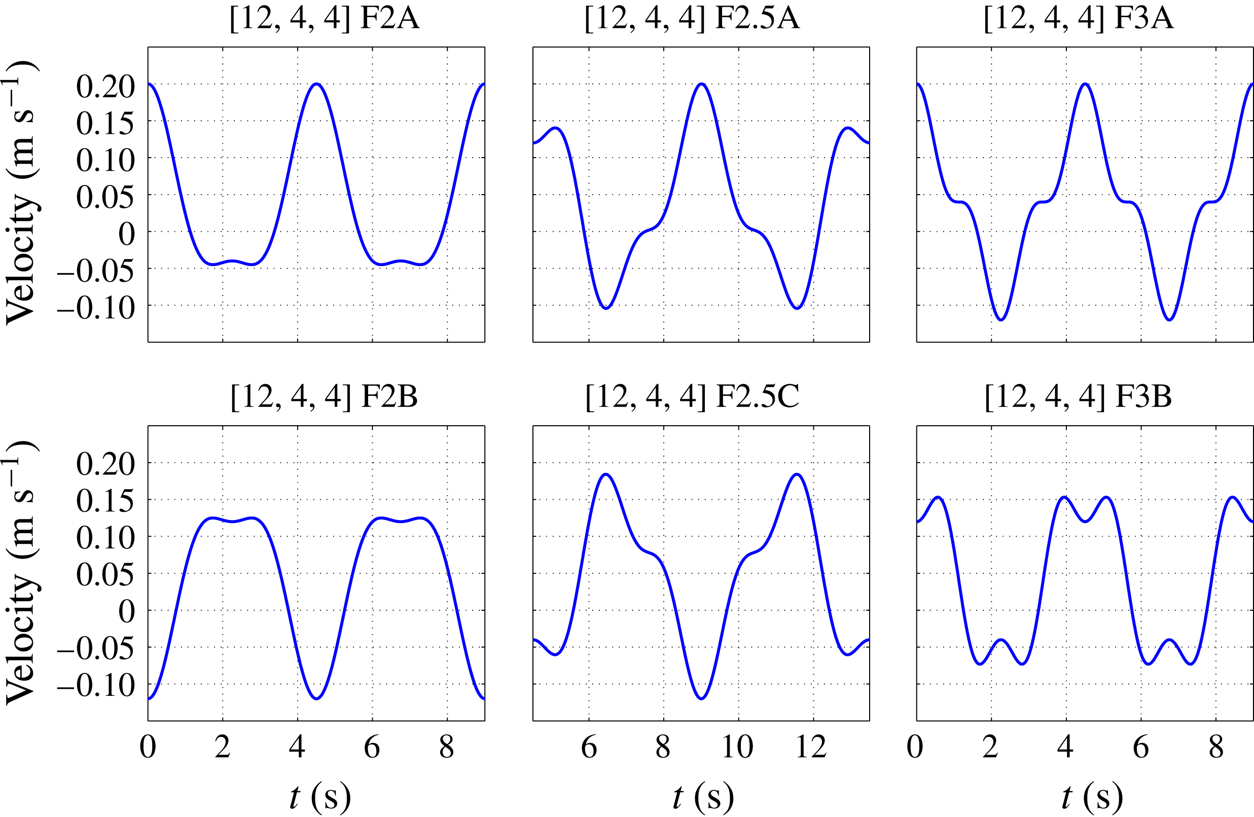
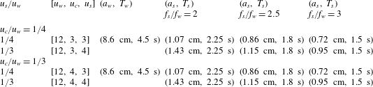
Table 2 summarises the test matrix, table 3 and figure 2 show the motion combinations (in terms of velocity–time history) presented in the paper. Throughout the paper, [
 $u_{w}$
,
 $u_{c}$
,
 $u_{s}$
] (in
 $\text{cm}~\text{s}^{-1}$
) followed by the motion label will be used as a naming convention to define each specific case.
Experimental parameters with ratio of
 $u_{s}/u_{w}$
and
 $u_{c}/u_{w}$
;
 $u_{w}$
,
 $u_{s}$
and
 $u_{c}$
in
 $\text{cm}~\text{s}^{-1}$
. Note that
 $a_{w}=$
wave oscillation amplitude,
 $T_{w}=$
wave oscillation period,
 $a_{s}=$
structural oscillation amplitude and
 $T_{s}=$
structural oscillation period.
Motion combinations for each
 $f_{s}/f_{w}$
. Note that F2 denotes
 $f_{s}/f_{w}=2$
and so on.

Plots of all motion combinations in terms of velocity–time history for an example case of [12, 4, 4].

2.3 A note on the force decomposition
The load signals measured from the force transducer are assumed to consist of both drag and inertia force components, which need to be separated for further analysis. Cycle-by-cycle averaging is first performed on the low-pass filtered load signals when the total force is in steady state (simply periodic – repeating every or every other wave cycle), removing the starting and ending transients. Typically the averaging is performed over ten wave cycles. Next, the force decomposition method described by Santo et al. (Reference Santo, Taylor, Williamson and Choo2014b ) is used to extract drag and inertia components from the total force.
The force decomposition relies on symmetry around the sinusoidal wave velocity (or surface elevation when free-surface fluctuation is present), and the method assumes the resultant drag force to be horizontally symmetric in shape around the peak drag, just like the imposed sinusoidal velocity. For oscillatory motions on two scales (wave oscillation and steady motion), the decomposition method is considered satisfactory as noted by Santo et al. (Reference Santo, Taylor, Williamson and Choo2014b ), although a slight asymmetry around the ‘shoulders’ (inflexion or zero crossing points) of the decomposed drag force was observed using Fourier decomposition. For oscillatory motions on three scales as considered here, however, there might be flow regions where there is a more pronounced asymmetry in the inferred drag force, and this limits further the adequacy of the force decomposition method as discussed in § 3.2.
3 Analytical modelling
For fluid loading on a drag-dominated structure where diffraction is not important, the flow and fluid loading fall into a Morison-type regime (defined as
 $D/\unicode[STIX]{x1D706}<0.2$
, where
 $D$
is the cylinder diameter and
 $\unicode[STIX]{x1D706}$
is the wavelength), as proposed first by Morison et al. (Reference Morison, O’Brien, Johnson and Schaaf1950). Several extensions to the standard form accounting for structural motion have been proposed based upon the concepts of independent flow (absolute velocity) and relative flow fields (relative velocity): see for example Shafiee-Far et al. (Reference Shafiee-Far, Massie and Vugts1996). In this paper, we focus on an extended model with relative velocity. For forced motion on three scales in otherwise still water, the standard Morison formulation expressed as a summation of drag and inertia force components is written as (see § 2.3.1.c of Recommended Practice RP2A of the American Petroleum Institute 2000):
 $$\begin{eqnarray}\displaystyle \text{Total Force} & = & \displaystyle {\textstyle \frac{1}{2}}\unicode[STIX]{x1D70C}C_{d}A(u_{w}\cos \unicode[STIX]{x1D714}t+u_{c}+u_{s}\cos n\unicode[STIX]{x1D714}t)|u_{w}\cos \unicode[STIX]{x1D714}t+u_{c}+u_{s}\cos n\unicode[STIX]{x1D714}t|\nonumber\\ \displaystyle & & \displaystyle -\,\unicode[STIX]{x1D70C}VC_{m}(\unicode[STIX]{x1D714}u_{w}\sin \unicode[STIX]{x1D714}t+n\unicode[STIX]{x1D714}u_{s}\sin n\unicode[STIX]{x1D714}t),\end{eqnarray}$$
where
 $C_{d}$
and
 $C_{m}$
are the Morison drag and inertia coefficients, respectively,
 $\unicode[STIX]{x1D714}t$
is the wave oscillation phase angle,
 $A$
is the solid drag area of the grid,
 $V$
is the displaced volume of the elements in the grids,
 $\unicode[STIX]{x1D70C}$
is the water density and
 $n=f_{s}/f_{w}$
is the frequency ratio, with
 $2n$
taken as integer.
While (3.1) has been used extensively in the past and may be applicable for a single member, such as a cylinder, the validity to a whole structure with multiple members has not been examined. Moreover, wave–current–structure blockage effects might be significant, and hence an extension to the blockage model having a different form to (3.1) might be needed.
3.1 Extended full current blockage theory
Previously, following Taylor et al. (Reference Taylor, Santo and Choo2013) and Santo et al. (Reference Santo, Taylor, Williamson and Choo2014b
), for the asymptotic limit of
 $u_{w}>>u_{c}$
, the wave–current blockage model for regular oscillation predicts that the drag force can be expressed as a summation of a wave drag term and a current drag term, as follows:
 $$\begin{eqnarray}\displaystyle & \text{Drag}=\displaystyle \frac{1}{2}\unicode[STIX]{x1D70C}C_{d}Au_{w}^{2}\cos \unicode[STIX]{x1D714}t|\cos \unicode[STIX]{x1D714}t|+\displaystyle \frac{\unicode[STIX]{x03C0}}{4}\unicode[STIX]{x1D70C}A_{f}u_{c}^{2}|\cos \unicode[STIX]{x1D714}t|, & \displaystyle\end{eqnarray}$$
where
 $A_{f}$
is the projected frontal area of the grid. Notice the absence of the
 $(u_{w}\times u_{c})$
term in the approximate form, and notice the current drag term contains a time dependent
 $|\text{cos}\unicode[STIX]{x1D714}t|$
, which is phase-locked to the wave velocity field yet scales with the current velocity squared.
Here, we aim to derive a similar expression for the approximate formulation with an additional structural oscillation,
 $u_{s}$
, and assess whether the relative-velocity formulation in the Morison-based blockage model is valid.
Consider now a grid in a flow with a locally blocked current
 $u_{cs}$
, a regular oscillating wave component
 $u_{w}$
and oscillating structural component
 $u_{s}$
. The frequency ratio between the two oscillating components is
 $n$
, with
 $2n$
assumed integer. Assuming that the Morison equation can be used to describe the force on the obstacles over the wave cycle and that there is no variation of
 $C_{d}$
with oscillation sweep position, the averaged force over a complete flow oscillation according to the wave–current–structure blockage model can be expressed as
 $$\begin{eqnarray}\displaystyle \displaystyle \frac{F_{av}}{\displaystyle {\textstyle \frac{1}{2}}\unicode[STIX]{x1D70C}C_{d}A} & = & \displaystyle \displaystyle \frac{1}{4\unicode[STIX]{x03C0}n}\int _{0}^{4\unicode[STIX]{x03C0}n}\displaystyle (u_{w}\cos \unicode[STIX]{x1D714}t+u_{s}\cos n\unicode[STIX]{x1D714}t+u_{cs})\nonumber\\ \displaystyle & & \displaystyle \times \,|u_{w}\cos \unicode[STIX]{x1D714}t+u_{s}\cos n\unicode[STIX]{x1D714}t+u_{cs}|\,\text{d}(\unicode[STIX]{x1D714}t).\end{eqnarray}$$
Previous analysis for forced oscillation on two scales showed that the integral has exact solutions for all flow regimes. In particular, for the asymptotic limit of
 $u_{w}\gg u_{c}$
, the average force reduces to
 $$\begin{eqnarray}\displaystyle \displaystyle \frac{F_{av}}{\displaystyle {\textstyle \frac{1}{2}}\unicode[STIX]{x1D70C}C_{d}A}\rightarrow \displaystyle \frac{4}{\unicode[STIX]{x03C0}}u_{cs}u_{w}. & & \displaystyle\end{eqnarray}$$
The integral for motions at three scales has no exact (closed-form) solution for arbitrary
 $n$
and velocity components, so we take the asymptotic limit of
 $u_{w}\gg u_{cs}$
and
 $u_{w}\gg |u_{s}|$
. The phase is defined relative to
 $u_{w}$
, and
 $u_{s}$
is either in phase or
 $\unicode[STIX]{x03C0}$
out of phase with a
 $u_{w}$
crest, determined by the sign of
 $u_{s}$
. Assuming that the number of total force zero crossings is the same as for
 $u_{s}=0$
per wave period, the following results are obtained:
 $$\begin{eqnarray}\displaystyle & \displaystyle \frac{F_{av}}{{\textstyle \frac{1}{2}}\unicode[STIX]{x1D70C}C_{d}A}\rightarrow \displaystyle \frac{4}{\unicode[STIX]{x03C0}}u_{cs}u_{w}\times [1+\cdots \,]. & \displaystyle\end{eqnarray}$$
The form of the leading-order term in this bracket depends on the frequency ratio
 $n$
.
When
 $n$
is an even integer, such as 2, 4 or 6, we have
 $$\begin{eqnarray}\displaystyle \left[1+\frac{-(-1)^{n/2}}{n^{2}-1}\frac{u_{s}}{u_{cs}}\right], & & \displaystyle\end{eqnarray}$$
when
 $n$
is an odd integer, such as 3, 5 or 7, we have
 $$\begin{eqnarray}\displaystyle \left[1+\frac{(-1)^{(n-1)/2}}{n}\frac{u_{s}}{u_{w}}\right], & & \displaystyle\end{eqnarray}$$
and when
 $n$
is a half-integer, such as
 $3/2,5/2$
or
 $7/2$
, we have
 $$\begin{eqnarray}\displaystyle \left[1+\frac{(-1)^{n-1/2}}{8n}\frac{u_{s}^{2}}{u_{cs}u_{w}}\right]. & & \displaystyle\end{eqnarray}$$
Thus, for
 $n$
both odd and half-integer, the extra contribution to the averaged force,
 $F_{av}$
(relative to (3.4)) scales as
 ${\sim}u_{s}u_{cs}$
and
 ${\sim}u_{s}^{2}$
, respectively. Both are much smaller and can be assumed negligible compared to the case for
 $n$
an even integer, in which case the extra contribution to
 $F_{av}$
now noticeably scales as
 $u_{w}u_{s}$
. Hence, in the analysis of the experiments it is expected that there may be two distinct force expressions required: for
 $n=2$
, and for all other cases such as
 $n=2.5$
and 3 where the new additional contributions are negligible, according to the blockage model.
We now relate the local expressions of (3.5) to the global reduction in the free-stream current at the grid. The result in terms of the net force on the actuator disc for the grid of the time-averaged mean flow can be used to describe the global reduction, which is written as
 $$\begin{eqnarray}\displaystyle & \displaystyle F_{av}=2A_{f}\unicode[STIX]{x1D70C}u_{cs}(u_{c}-u_{cs}). & \displaystyle\end{eqnarray}$$
The above expression can be obtained by considering a streamtube flow over an actuator disc with stable vortex sheets separating the wake from the external flow downstream. Describing the flow globally, the approaching free-stream flow velocity (
 $u_{c}$
) is reduced to a shielded flow velocity (
 $u_{cs}$
) due to the disc. There is an associated pressure drop across the disc, which gives rise to the net drag force on the disc. Downstream of the grid, the flow velocity drops further in the far wake region, while the pressure slowly rises back to the ambient pressure. Thus, one can apply conservation of energy upstream and downstream of the disc, as well as conservation of momentum across the disc, to recover (3.9).
We then retain the concept of partitioning the total drag force into a two-disc model. The front disc is assumed to block the mean flow (mainly
 $u_{c}$
) completely (the current drag term), leaving the rear disc exposed to oscillatory flow only (the wave drag term). Such an assumption is justified from the reasonably good agreement between the model prediction and experimental measurements for forced motion on two scales using the same grid set-up as outlined in Santo et al. (Reference Santo, Taylor, Williamson and Choo2014b
). By relating (3.5)–(3.9) and equating
 $u_{cs}=u_{c}/2$
, the allowable hydrodynamic loading,
 $C_{d}A_{L}/A_{f}$
on the front disc can be obtained, with the remaining hydrodynamic loading,
 $C_{d}(A-A_{L})/A_{f}$
apportioned to the rear disc. Substituting both expressions of the hydrodynamic loading into the two-disc model, the following (3.11) will be recovered. Hence, our approximate model for the wave–current–structure blockage is based on the asymptotic two-disc model result of the wave–current blockage model with additional modification to allow for contributions from the structural oscillation,
 $u_{s}$
.
Interestingly, when
 $n$
is an even integer, there is an additional mean force contribution even in the absence of a current, i.e. when
 $u_{cs}=0$
. The general form of the additional mean force is expressed as
 $$\begin{eqnarray}\displaystyle \displaystyle \frac{F_{av}}{{\textstyle \frac{1}{2}}\unicode[STIX]{x1D70C}C_{d}A}\rightarrow \displaystyle \frac{-4(-1)^{n/2}}{(n-1)(n+1)\unicode[STIX]{x03C0}}u_{s}u_{w}\left[1-\displaystyle \frac{(n-1)(n+1)}{6}\left(\displaystyle \frac{u_{s}}{u_{w}}\right)^{2}\right]. & & \displaystyle\end{eqnarray}$$
This then poses a slight incompatibility in the application of the two-disc model, in particular for
 $n=2$
. This is dealt with below.
The approximate form for drag and the exact form for inertia according to the wave–current–structure blockage model is expressed as
 $$\begin{eqnarray}\displaystyle & \left.\begin{array}{@{}c@{}}\displaystyle \text{Drag}=\text{Drag}_{w}-\overline{\text{Drag}_{w}}+\text{Drag}_{c}\\ \displaystyle \text{where Drag}_{w}=\displaystyle \frac{1}{2}\unicode[STIX]{x1D70C}C_{d}A(u_{w}\cos \unicode[STIX]{x1D714}t+u_{s}\cos n\unicode[STIX]{x1D714}t)|u_{w}\cos \unicode[STIX]{x1D714}t+u_{s}\cos n\unicode[STIX]{x1D714}t|\\ \displaystyle \text{Drag}_{c}=\displaystyle \frac{\unicode[STIX]{x03C0}}{4}\unicode[STIX]{x1D70C}A_{f}(u_{c}^{2}+u_{s}|u_{s}|)|\text{cos}\unicode[STIX]{x1D714}t|\quad (\text{for }n=2)\\ \displaystyle \text{ Drag}_{c}=\displaystyle \frac{\unicode[STIX]{x03C0}}{4}\unicode[STIX]{x1D70C}A_{f}u_{c}^{2}|\text{cos}\unicode[STIX]{x1D714}t|\quad (\text{for }n=2.5\text{ and }3)\end{array}\right\} & \displaystyle\end{eqnarray}$$
 $$\begin{eqnarray}\displaystyle & \displaystyle \text{Inertia}=-\unicode[STIX]{x1D70C}VC_{m}(\unicode[STIX]{x1D714}u_{w}\sin \unicode[STIX]{x1D714}t+n\unicode[STIX]{x1D714}u_{s}\sin n\unicode[STIX]{x1D714}t). & \displaystyle\end{eqnarray}$$
Although the model is developed for
 $u_{w}\gg u_{c}$
, it is also valid when
 $u_{c}=0$
, when the model reduces to a simple Morison equation with the relative-velocity formulation.
Note that the structural oscillation is included in the unsteady wave drag term (
 $\text{Drag}_{w}$
), and an offset to the mean force term (
 $\overline{\text{Drag}_{w}}$
) due to the wave drag term is introduced. For
 $n=2$
particularly, the wave drag term resulting from oscillation at three scales contains a significant mean force when integrated over a wave cycle (see (3.10)), which should not be there because the front disc has been assumed to take out the mean force completely. Hence, the offset term is introduced for consistency, and the current drag term (
 $\text{Drag}_{c}$
) for
 $n=2$
contains an additional mean force term due to structural oscillation, with a modulus sign on the velocity term to account for the relative phase between the wave and structural oscillations (in phase or out of phase). For
 $n=2.5$
and 3, the same current drag term as in (3.2) is retained, and the wave drag term contains negligible mean force.
The inertia term follows the standard Morison inertia term with a single
 $C_{m}$
and with an additional acceleration of the structural motion. Note that because the Morison equation is usually expressed in terms of the undisturbed flow field, in our experiments of forced oscillations there is no convective acceleration term (
 $\unicode[STIX]{x2202}u/\unicode[STIX]{x2202}x$
) for the undisturbed flow field, hence the inertia term in this case contains only the
 $\unicode[STIX]{x2202}u/\unicode[STIX]{x2202}t$
term.
3.2 Forms and comparison of the force–time histories
We first perform curve fitting on the measured drag and inertia force components using (3.11) and (3.11) by minimising the mean square error, consistent with previous data analyses by Santo et al. (Reference Santo, Taylor, Williamson and Choo2014b
). The objective is to obtain the best fit of Morison drag and inertia coefficients for each test case. Since most of the drag force–time histories contain less severe inflexion (shoulder) at the zero crossing compared to the analytical prediction, a weighting function of
 $\text{cos}^{1000}(\unicode[STIX]{x1D714}t)$
is introduced to force the minimisation to occur only at narrow regions around both crests and troughs of the drag force. The only exception is for the case of F3B where no distinct crests and troughs of the drag force are observed, hence no weighting function is used for this particular case. No weighting function is applied for the inertia force error minimisation.
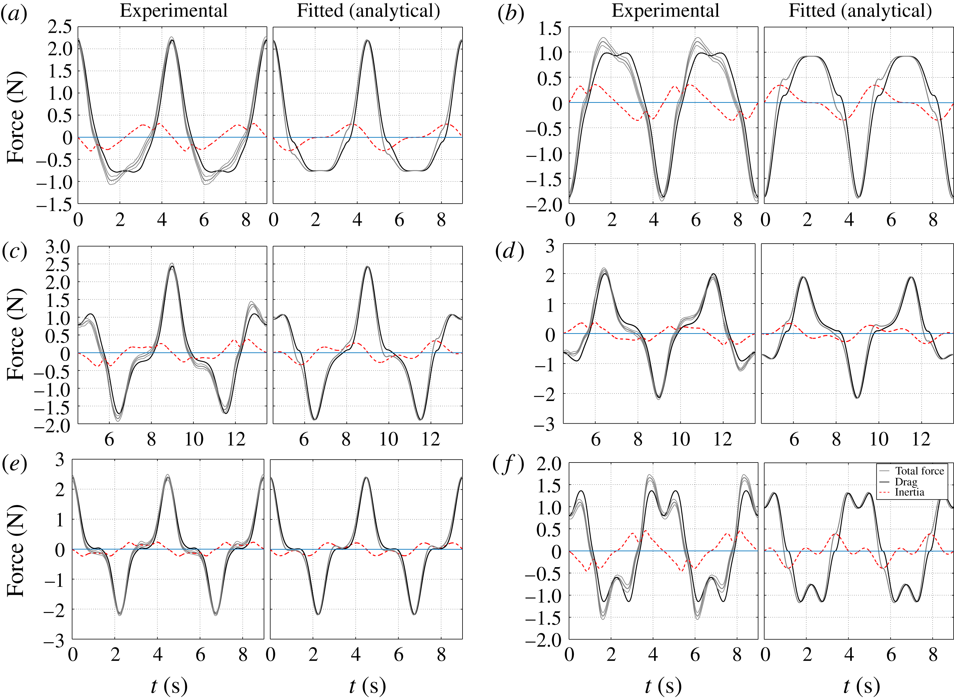
We present an example of the force–time history comparison for the case [12, 4, 3] as shown in figure 3, with experimental results in the left column of each panel and analytical predictions using (3.11) and (3.12) in the right column. Relatively good agreement is observed for the drag force comparison. There is however some discrepancy in the inertia force comparison, where the decomposed measured inertia force shows relatively smoother variation compared to the analytical inertia prediction. As a result, some of the total force–time histories are less well reproduced analytically when the inertia force is almost as important as the drag force, such as in figure 3(f). For most of the cases considered however, the drag force is significantly larger than the inertia force.
Comparison of force components between experimental (left column of each panel) and analytical results (right column of each panel) for six different combinations of [12, 4, 3]: (a,b) F2A and F2B, (c,d) F2.5A and F2.5C and (e,f) F3A and F3B. The thin grey lines represent error bars (
 $\pm$
2 standard deviation for the variation of the mean of the measured total force). Label A denotes the wave and structure velocity peaks in phase, B those out of phase and C
 $\unicode[STIX]{x03C0}/2$
-phase-shifted.

To indicate the amount of variability in the measured forces, thin grey lines are added to the same figure which represent
 $\pm$
2 standard deviations for the variation of the mean signal from the individual total force signals. As is apparent from the figure, there is good repeatability of the measured total forces judging from the tight band of the standard deviation. For the cases presented in the same figure, the average root mean square error of the measured total force is
 ${\sim}0.05$
N, and the average normalised root mean square error, defined as the root mean square divided by the range of the measured total force for each case, is
 ${\sim}1\,\%$
.
It is of interest to investigate the shape of the inertia term, which could be due to contributions from the higher harmonic components (higher than
 $f_{s}/f_{w}=2$
, 2.5 and 3), or due to the possibility of the measured drag force not being symmetric in time. We could possibly obtain a much better fit to the inertia term if two different
 $C_{m}$
values were used for the wave and structural accelerations in (3.11). However, there is no theoretical justification for this because the inertia force is assumed to be associated with potential flow perturbations and hence there should be no difference in the resultant inertia contributions for the two oscillations.
Although the force signals are initially low-pass filtered at
 $12\times$
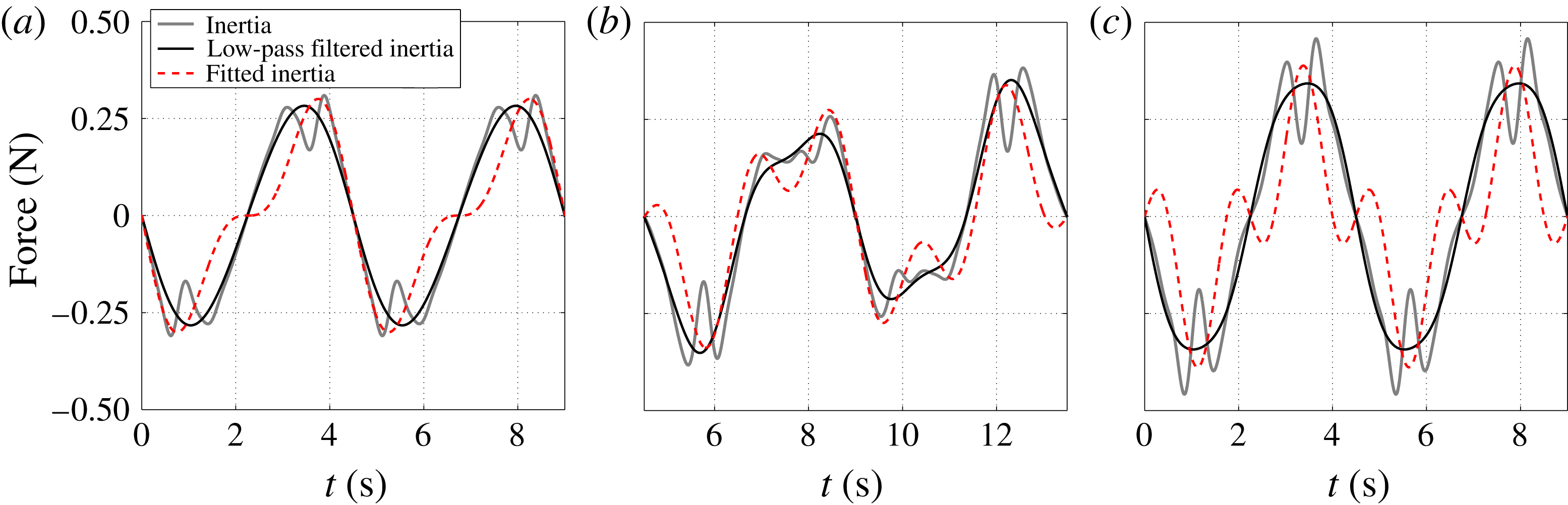
the frequency of the oscillatory wave motion, it is important to identify the correct range of the driving frequency of structural oscillation when interpreting the measured force. We examine the contribution from the higher harmonics using frequency filtering. Figure 4 presents presumed inertia force components of some of the cases presented in figure 3. The measured inertia is low-pass filtered at a frequency larger than
 $f_{s}$
of each case, leaving behind the sum of the linear component associated with wave oscillation and the higher frequency component associated with structural oscillation. As is apparent from the figure, there is still a fundamental difference between the filtered (measured) inertia and the fitted inertia, in that the filtered inertia contains quite significant first and higher harmonic terms which could be regarded as leakage from the drag force. Drag asymmetry is a plausible explanation.

Here we explore the possibility of drag asymmetry using a combination of experimental data as well as numerical modelling (which will be presented in the next section). Santo et al. (Reference Santo, Taylor, Williamson and Choo2014b ) previously observed a slight asymmetry in the measured drag force around the inflexions (shoulders or zero crossing points) which was probably due to wake-related features associated with the physical grids, while the analytical Morison-based blockage model is still based on a symmetry assumption.
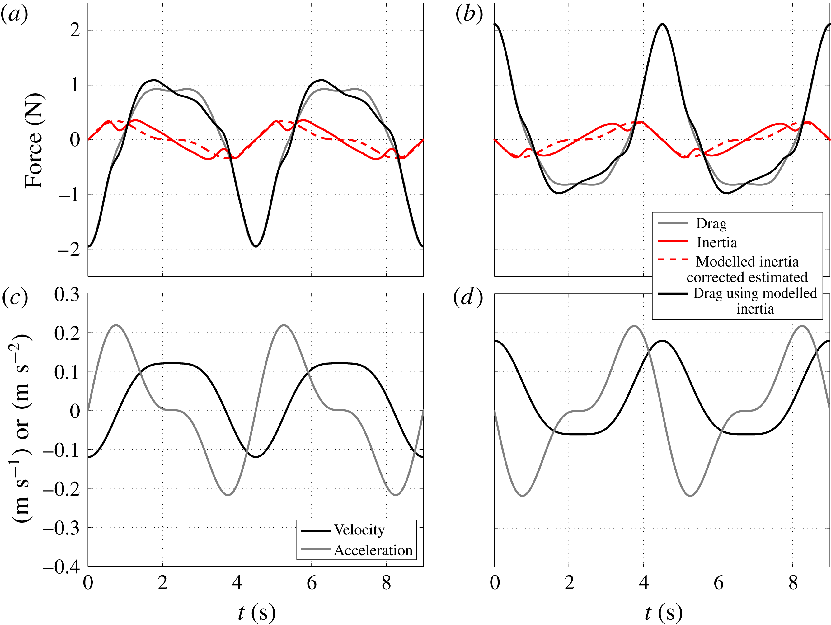
Figure 5 investigates the possible drag force asymmetry for the same cases of [12, 4, 3], F2B (a,c) and F2A (b,d). Figure 5(a,b) shows the measured averaged forces which have been decomposed into drag and inertia components, and figure 5(c,d) shows the corresponding velocity and acceleration. Using the symmetric force decomposition method, the resultant measured drag force is symmetric around the peak crest/trough of the velocity, while the resultant measured inertia force is closer to sinusoidal in time. The largest difference is observed around the ‘plateau’ (defined as relatively flat or constant motion) of the velocity signal (and the associated drag force). Since there is no theoretical justification for the use of different
 $C_{m}$
values for the wave and structural accelerations nor should the measured inertia force behave differently from the imposed fluid acceleration, the measured drag force is speculated to contain asymmetry around the ‘plateau’. The corrected measured drag force can be inferred by subtracting the fitted inertia term from the measured total force. This is shown as a solid black line in the top panel for each case. Comparing the two inferred drag forces, one can see that for the asymmetric drag force, the shoulders (inflexion points) are shifted, but the peak forces remain unchanged.
Examples of test cases which exhibit possible drag force asymmetry when the superimposed motions at three scales contain a ‘plateau’. (a,b) Measured averaged force components. (c,d) Corresponding velocity and acceleration. The cases belong to [12, 4, 3], F2B (a,c) and F2A (b,d).

This speculation is supported from the observation of steady tow results from Santo et al. (Reference Santo, Taylor, Williamson and Choo2014b
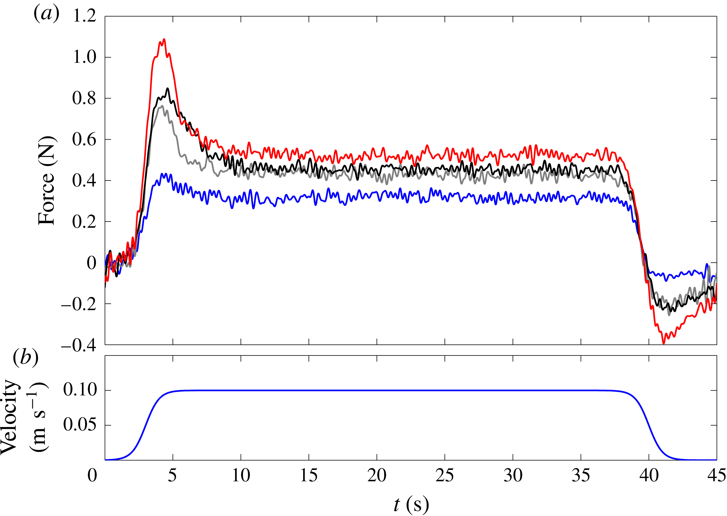
), re-plotted over a longer time scale in figure 6. Although the motion is predominantly steady, a transient effect of the initial and ending stage of the motion is observed during the ramp-up of the motions, and hence the measured total force contains not just steady drag but also inertia force contributions. When the time
 ${>}5$
s, the imposed velocity is steady (hence the acceleration is zero), but the measured force which should now contain only the drag force is still decaying in time, likewise when time
 ${>}42$
s. Hence, it is reasonable to assume that the drag force is asymmetric in shape (decaying from initial transient) when the imposed motion contains a ‘plateau’, and when the motion is periodic in time, the decaying asymmetric shape of the drag force is also simply periodic in time (repeating every cycle). It is interesting to note that the flow and hence force relaxation takes about 4 s from the instant when the imposed velocity is steady (e.g. from time
 $=$
5–9 s). For the imposed velocity of
 $10~\text{cm}~\text{s}^{-1}$
, this corresponds to 40 cm, which is just longer than the layout length of the three grids (30 cm).
Steady flow measurements of
 $u_{c}=10~\text{cm}~\text{s}^{-1}$
for grids with
 $A/A_{f}=0.45$
. (a) Measured force–time history, with different lines corresponding to different grid arrangements from a total of 1, 2 and 3 grids. (b) Imposed velocity–time history.

Drag asymmetry may occur when there is a biasing from the mean flow, i.e. instead of the flow simply oscillating to and fro, the flow tends to oscillate while moving preferentially one way. As in Santo et al. (Reference Santo, Taylor, Williamson and Choo2014b ), no prominent biasing flow was observed because the imposed flow is dominated by a single sinusoidal wave oscillation sweeping to and fro. In the present experiments, the additional structural oscillation contributes to the possibility of biasing from the mean flow in some of the flow combinations: mainly F2A, F2B and F3B motions. Because biasing from the mean flow is a wake-related effect, the drag force is affected by wake-related flow structures. Such effects are not included in the standard Morison equation (Morison et al. Reference Morison, O’Brien, Johnson and Schaaf1950), nor in our Morison-based blockage model which assumes drag force symmetry.
3.3 Forms of the measured force harmonics
For dynamically responding structures, the flow-excited motion of the structure is of interest, thus it is important to correctly represent the harmonic force component that is related to the structural oscillation. Hence, we investigate the adequacy of the proposed (3.11) and (3.12) in capturing the required force harmonics for dynamics response. To extract such force harmonics, frequency-by-frequency filtering is used.
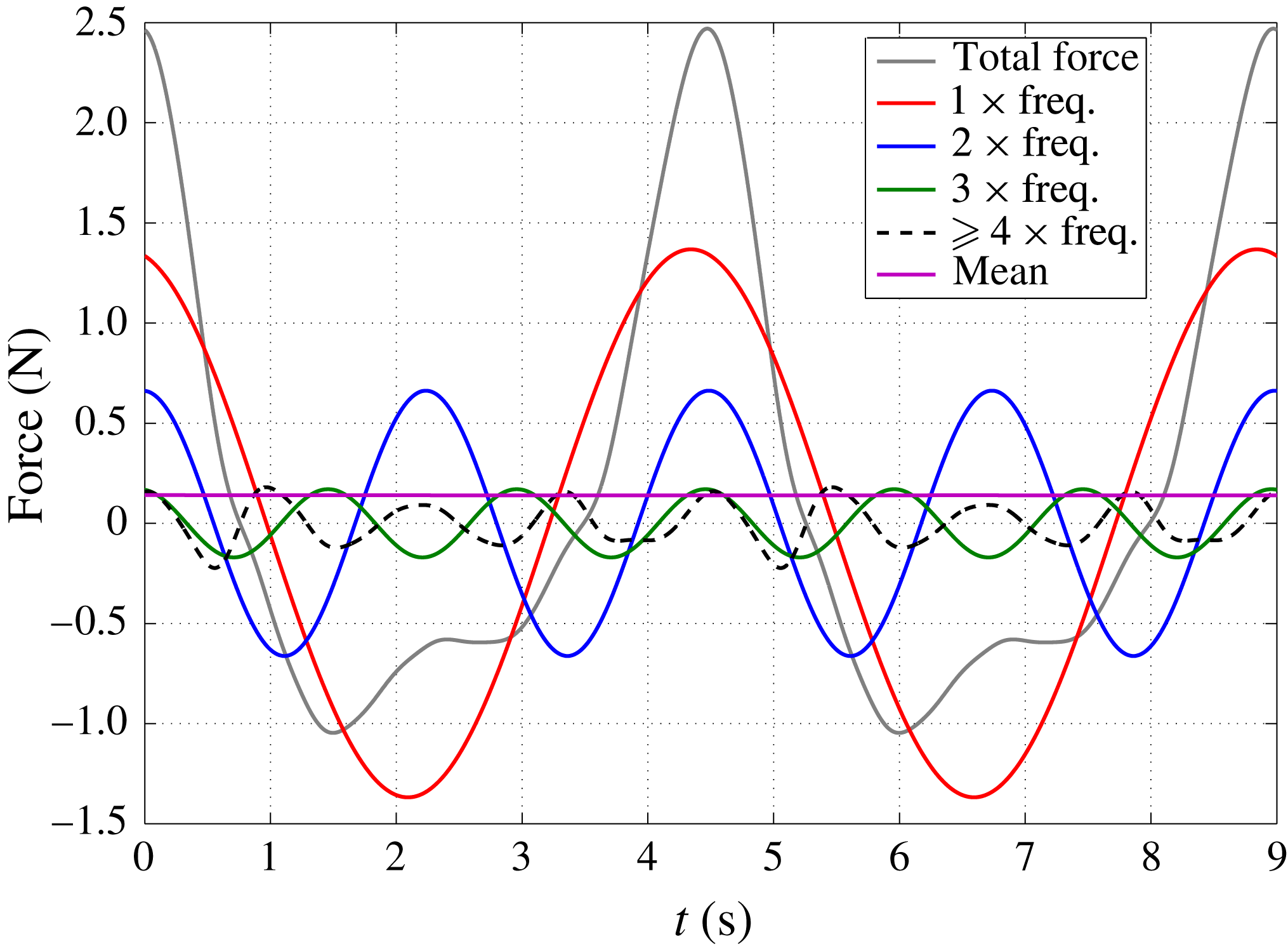
Figure 7 presents an example of narrow frequency filtering applied to the measured total force–time history for the case of [12, 4, 4] F2A. Narrow frequency filtering is justified because of the periodic response. The measured total force produces harmonics at each integer multiple of the dominant wave frequency, and each of the harmonics are filtered properly as can be seen from the corresponding force–time history. The same filtering process is applied to the experimental and analytical results of total force, drag and inertia force components of all cases. In the following, the forms of the measured force harmonics for
 $f_{s}/f_{w}=2$
and 3 with both in-phase and out-of-phase oscillations will be described. The forms and behaviour of the force harmonics for
 $f_{s}/f_{w}=2.5$
are similar to those for
 $f_{s}/f_{w}=3$
.
Example of narrow frequency filtering applied to the measured total force for the case of [12, 4, 4] F2A. The total force is shown as the solid grey line, linear frequency component as the solid red line, double frequency component as the solid blue line, mean force as the solid magenta line, triple frequency component as the solid green line and fourth frequency component and beyond as the dashed black line.

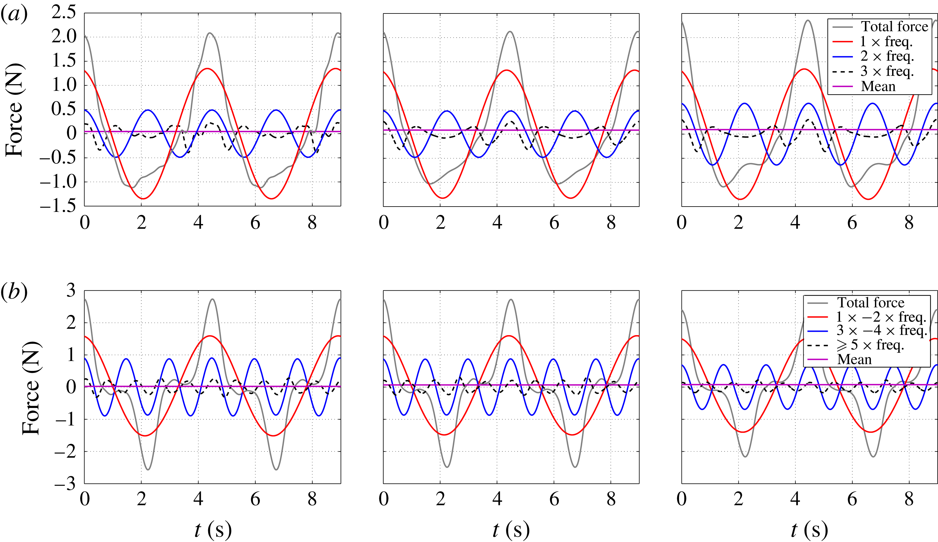
Comparison of harmonic contributions of measured total force–time histories: (a) [12, 0, 3] (left), [12, 3, 3] (middle) and [12, 3, 4] (right), all with F2A motion; (b) [12, 0, 4] (left), [12, 4, 4] (middle) and [12, 4, 3] (right), all with F3A motion.

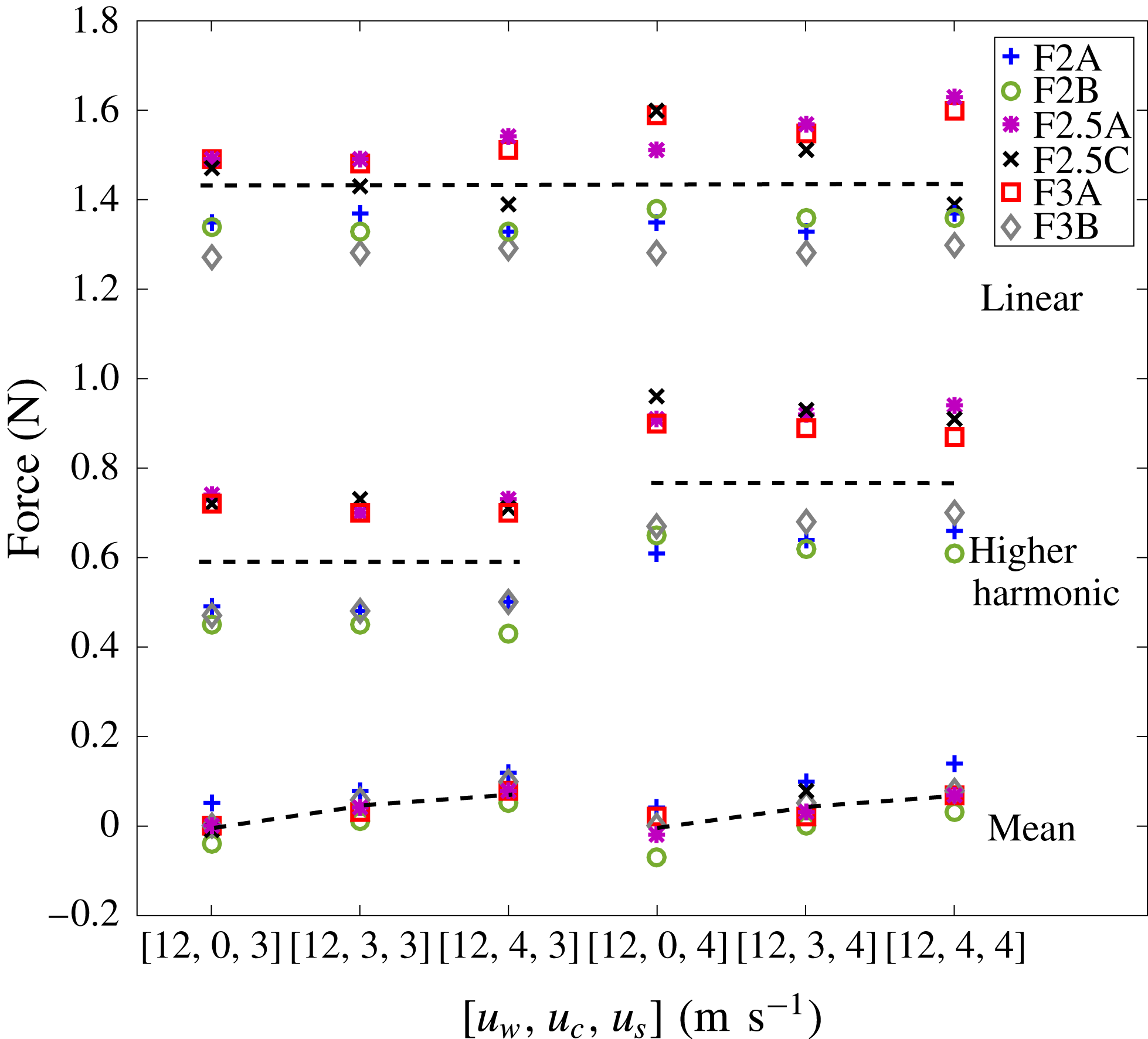
Plots of the variation of the peak force harmonics in terms of mean force, linear and higher harmonics for all the cases. The dashed lines are the suggested trendlines.

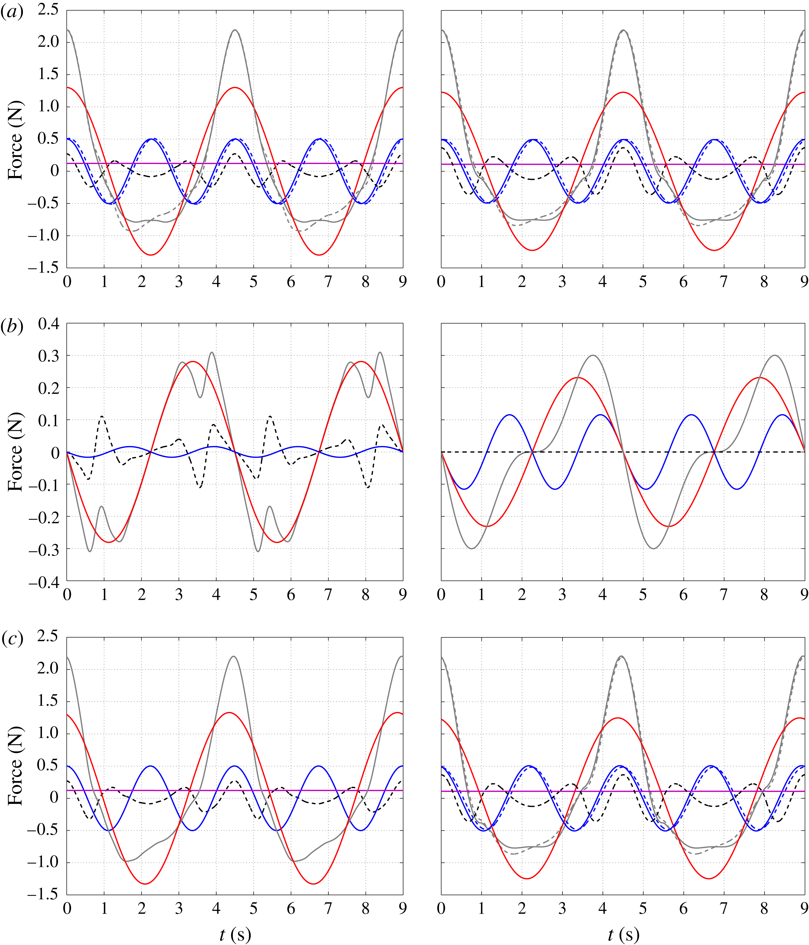
Comparison between experimental (left) and analytical results (right) for the case of [12, 4, 3] F2A in terms of harmonic contributions of (a) drag force, (b) inertia force and (c) total force. The total signal is shown as solid grey line, linear frequency component as solid red line, double frequency component as solid blue line, mean force as solid magenta line and triple frequency component and beyond as dashed black line. The dashed grey and blue lines are the modified total signal and the modified double frequency component, respectively.

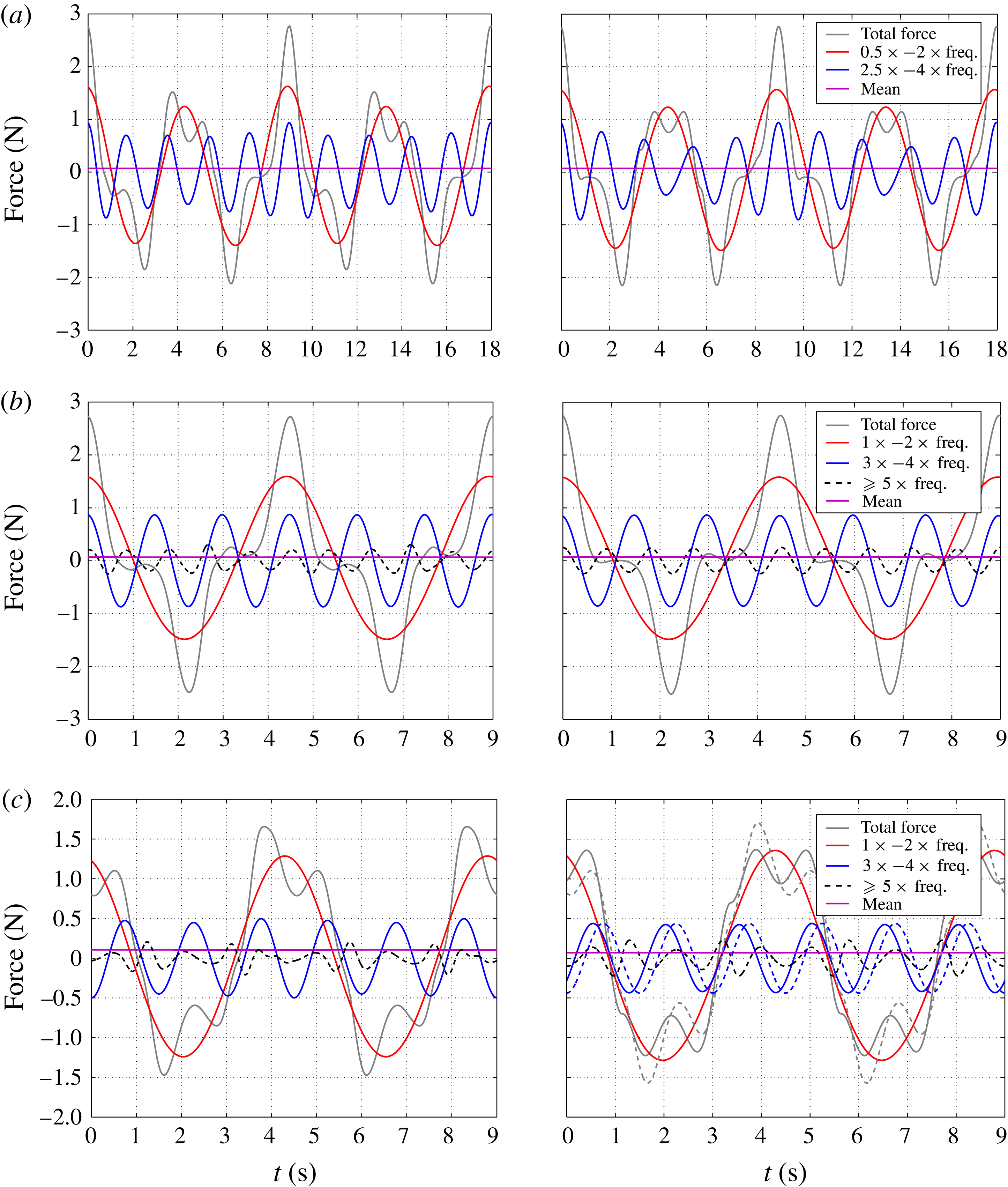
Comparison between experimental (left) and analytical results (right) for the case of (a) [12, 4, 4] F2.5A, (b) [12, 4, 4] F3A and (c) [12, 4, 3] F3B.

Figure 8(a) illustrates an example of F2A motion whereby the total force has been decomposed into the harmonic contributions for the case of [12, 0, 3] (left), [12, 3, 3] (middle) and [12, 3, 4] (right). Comparing the cases without and with current, i.e. between [12, 0, 3] and [12, 3, 3], there is hardly any change in the linear, double and triple frequency components, but the mean force increases as the current is introduced. The odd harmonics scale with
 $u_{w}$
only, hence the linear and triple frequency components hardly change for all cases with
 $u_{w}$
fixed. The zeroth frequency (mean force) of the first even harmonic scales with a combination of
 $u_{s}$
and
 $u_{c}$
. Hence, in the absence of
 $u_{c}$
there is still a mean force in [12, 0, 3], which demonstrates why the wave drag term, as presented in (3.11), contains a mean force when integrated over a wave cycle. The mean force increases slightly from [12, 3, 3] to [12, 3, 4]. The subsequent even harmonic term however scales with
 $u_{s}$
only, hence the double frequency component of [12, 0, 3] is unchanged when
 $u_{c}$
is introduced but increases as
 $u_{s}$
increases. Similar behaviour is observed for F2B motion.
Figure 8(b) provides an example of F3A motion. From the Fourier-transformed amplitude spectrum (not shown), the odd harmonics are dominant over the even harmonics, which is expected for the
 $f_{s}/f_{w}=3$
case. For presentational purposes, each of the even harmonics is paired with the adjacent odd harmonic; for instance the double frequency term is grouped together with the linear frequency component, and so on. The odd harmonics scale with a combination of
 $u_{w}$
and
 $u_{s}$
, in that the linear frequency component hardly changes for all cases of
 $f_{s}/f_{w}=3$
(only scales with
 $u_{w}$
), and the triple frequency component changes with different
 $u_{s}$
. The even harmonics, including the mean force, approximately scale with
 $u_{c}$
only. Increasing the current only produces an observable increase in the mean force. Similar behaviour is observed for F3B, F2.5A and F2.5C motions.
Figure 9 provides a quantitative measure of the trend of the peak values of the force harmonics (in terms of mean force, linear and higher harmonics). To summarise, for all cases with fixed
 $u_{w}$
, the linear frequency components scale as
 $u_{w}$
, and the higher harmonic components (driven by the structural oscillation) scale as
 $u_{s}$
. However, the mean force scales as either a combination of
 $u_{c}$
and
 $u_{s}$
for F2 motions, or as
 $u_{c}$
only for the remaining motions.
3.4 Comparison of the force harmonics
Figure 10 shows the drag, inertia and total force harmonic comparisons for [12, 4, 3] F2A. The drag force can be decomposed into a summation of both odd and even harmonics beyond the imposed oscillation frequency (figure 10 a). The peak harmonic force components are reasonably well represented by the analytical model, including the mean, linear frequency, double frequency and triple and higher frequency components. The analytical inertia force can be decomposed into a summation of the linear and double frequency components, whereas the measured inertia (inferred using the symmetry argument) has a more complicated structure (figure 10 b). The linear term of the measured inertia force is larger than the analytical prediction, but the double frequency term is reduced and the triple and higher frequency terms are quite significant. As described previously in § 3.2, the inferred measured inertia could be distorted because of the force symmetry assumption invoked in the force decomposition. Although the drag force is reasonably well represented but the inertia force is not, it is worth emphasising that the experimental drag and inertia are obtained using force decomposition by assuming symmetry around the peak drag; the actual shape of the measured drag and inertia components are unknown if drag asymmetry is significant.
The total force comprising drag and inertia is shown to contain all the force harmonics (figure 10
c). The total force is measured directly, and so the comparison in terms of total force signal is perhaps the most straightforward to test the adequacy of the proposed analytical wave–current–structure blockage model. As is apparent from the figure, the peak forces of each harmonic agree relatively well from linear to higher harmonic terms. Overall, relatively good agreement is obtained in each of the harmonic contributions, which demonstrates the adequacy of the proposed (3.11) and (3.12) in describing the total force–time history for
 $f_{s}/f_{w}=2$
. Similar agreement is obtained for the remaining F2A and F2B cases. The analytical form is based on the drag symmetry assumption, and so the largest discrepancy persists owing to the strong asymmetry exhibited in the measured total force. It is apparent from figure 10 that the harmonic components higher than the double frequency (which is the imposed structural oscillation frequency,
 $f_{s}$
) do not contribute to the force asymmetry as the peak and the phase are relatively well represented.
The real difference in the total force comparison shown in figure 10(c) is the phase of the double frequency component. There is a slight phase difference in that the crest of the double frequency component of the measured total force is aligned closer to that of the higher harmonic component than the analytical counterpart. It is this phase shift that contributes to the force asymmetry, and the larger the phase shift the more pronounced the force asymmetry.
Although the actual shapes of the measured drag and inertia force are not known, the actual shape of the drag force can be approximated by inferring from the total force, assuming the actual inertia force is behaving according to the potential-flow prediction. This is performed for the measured drag force shown in figure 10(a): no obvious changes to the rest of the harmonics occur other than a rather obvious phase shift of 0.1 rad (6
 $^{\circ }$
) in the double frequency component. The same amount of phase shift is applied to the double frequency component of the analytical drag force, and a modified drag and total force, which both exhibit strong asymmetry, are obtained. Having accounted for the drag force asymmetry, the comparison in terms of the total force is now better. Thus, in principle, the drag asymmetry due to biasing from the mean flow can be modelled with a phase shift to the double frequency harmonic term for
 $f_{s}/f_{w}=2$
.
Figure 11(a) shows the comparison of [12, 4, 4] F2.5A, with the harmonics presented up to
 $2.5-4\times$
the dominant (wave) frequency band. The time axis has been doubled to 18 s for clarity. The peak values of the harmonics are reasonably well predicted by the analytical modelling especially around the crests and troughs of the total force. There are however some phase differences in the harmonics around the plateau (such as
 ${\sim}4$
s), which contribute to force asymmetry. The triple frequency component, as predicted by the analytic form, is more dominant than the measured counterpart, and that component distorts the resultant shape of the
 $2.5-4\times$
frequency band component around the plateau. The harmonic comparison is considered satisfactory. Similar observations also apply for the remaining F2.5A and F2.5C cases. Figure 11(b) presents the comparison of [12, 4, 4] F3A. In general, both the peak values and the phases of all the predominantly odd harmonics are well represented by the analytical form, and there is no obvious force asymmetry around the force plateau. Reasonably good agreement is achieved for the remaining F3A cases.
Figure 11(c) shows the comparison of [12, 4, 3] F3B. Initially, the harmonics are not well represented analytically because the analytical fitting was performed without any weighting function imposed since there are no distinct crests and troughs in the force traces (drag and/or inertia). Trial and error is then conducted to obtain the best fit to the measurements in terms of force harmonics, mainly the first two odd harmonic terms. Better agreement is obtained after increasing the fitted inertia force previously shown in figure 3 by
 $1.8\times$
while maintaining the same fitted drag force, as shown in the present figure. Reasonably good agreement is observed in terms of peak values, although both the mean force and triple frequency harmonic terms are slightly under-predicted. From the measured total force–time history, it is apparent that force asymmetry is quite severe around the force plateau, akin to
 $f_{s}/f_{w}=2$
. A closer investigation reveals that there is a phase difference in the triple frequency harmonic component, which may be related to biasing from the mean flow. Applying the same phase shift to the fitted triple frequency harmonic term, a modified fitted total force is obtained which compares much better with the measured total force. Therefore, similar to
 $f_{s}/f_{w}=2$
, the force asymmetry can be effectively modelled by introducing a phase shift to the force harmonics primarily driven by the structural oscillation.
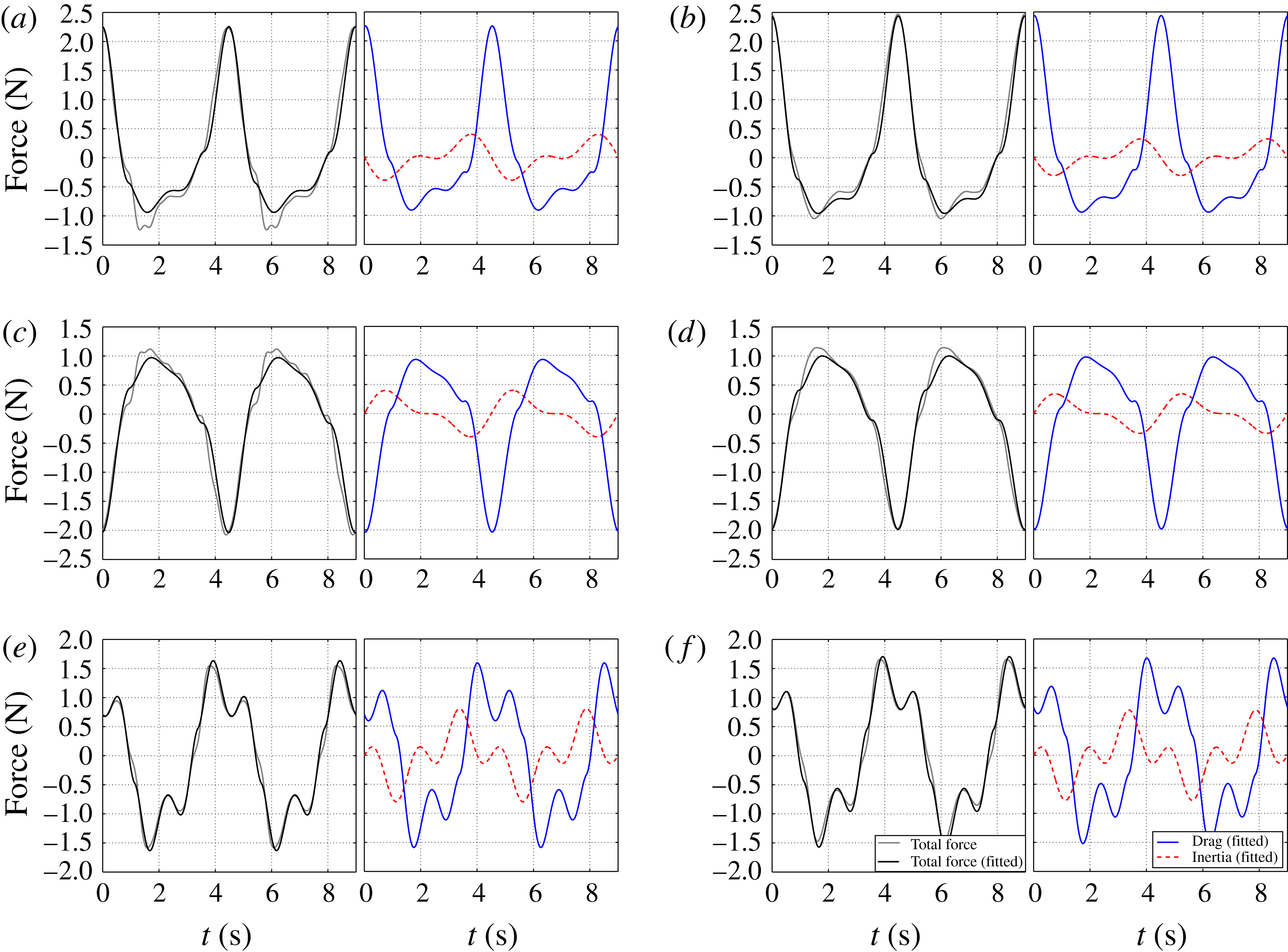
Comparison of total force–time history (left column of each panel) and fitted drag and inertia force–time history (right column of each panel) for (a,b) [12, 0, 4] (left) and [12, 4, 4] (right) both with F2A motion, (c,d) [12, 0, 3] (left) and [12, 3, 3] (right) both with F2B motion, and (e,f) [12, 0, 3] (left) and [12, 4, 3] (right) both with F3B motion.

Figure 12 presents comparisons of the total force–time histories (left column of each panel) using the analytical model accounting for a force asymmetry for several cases of F2A, F2B and F3B. The fitted drag and inertia force–time histories are shown on the right column of each panel. Relatively good agreement is obtained for all presented cases, as well as all the remaining cases. Hence, although the
 $C_{d}$
and
 $C_{m}$
fitting is performed based on the assumption that the measured drag force is in phase with the imposed velocity and hence symmetric in time, the fitted total force according to (3.11) and (3.12) compares relatively well with the measurement, and the comparison is improved when (drag) force asymmetry is accounted for artificially. It is apparent that the analytical predictions now capture much of the dominant force harmonics, and that the remaining discrepancy between measurement and analytical predictions is largely due to harmonic contribution higher than the harmonics driven by the structural oscillation. Comparing figure 12 to figure 3, the analytical model given by (3.11) and (3.12) gives results that agree reasonably well with the measured data in all cases, regardless of whether a phase shift or zero phase shift is imposed on the higher harmonic component of the fitted drag term.
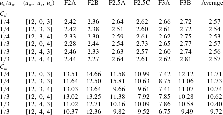
Table 4 in appendix B lists the
 $C_{d}$
and
 $C_{m}$
coefficients inferred from curve fit minimisation of the analytical model for all the test cases. It can be observed that the
 $C_{d}$
values are remarkably uniform for all cases presented, with a mean value of
 $C_{d}=2.56\pm 6\,\%$
. There is however more variation in the
 $C_{m}$
values, with a mean value of
 $C_{m}=10.82\pm 20\,\%$
. For cases with different
 $KC$
values (i.e. different
 $u_{w}/u_{s}$
,
 $f_{s}/f_{w}$
and
 $\unicode[STIX]{x1D719}$
), some of the variations are probably due to
 $KC$
number effects on each individual flat bar. For cases with the same
 $KC$
value, some of the variations are perhaps due to the curve fitting of the measured inertia component whereby the exact location of the peak inertia values is rather ambiguous, especially when the superimposed motions contain a plateau (see figure 4). Therefore, a larger variation in
 $C_{m}$
values could be expected. The variation in
 $C_{d}$
values is smaller because the peak drag component coincides with the zero crossing of the inertia component, and the location of the zero-crossing is less ambiguous compared to the location of the peak values. The values for
 $C_{d}$
and
 $C_{m}$
are relatively high, consistent with Santo et al. (Reference Santo, Taylor, Williamson and Choo2014b
), mainly because no corrections have been made for the presence of all the other obstacles in the grids while the Morison
 $C_{d}$
and
 $C_{m}$
are usually defined for an obstacle in isolation in a mean flow. Also, the
 $C_{d}$
and
 $C_{m}$
values for
 $f_{s}/f_{w}=3$
are found to be slightly different from the rest of the cases since this frequency ratio coincides with the triple harmonic contribution from the Morison
 $u|u|$
term.
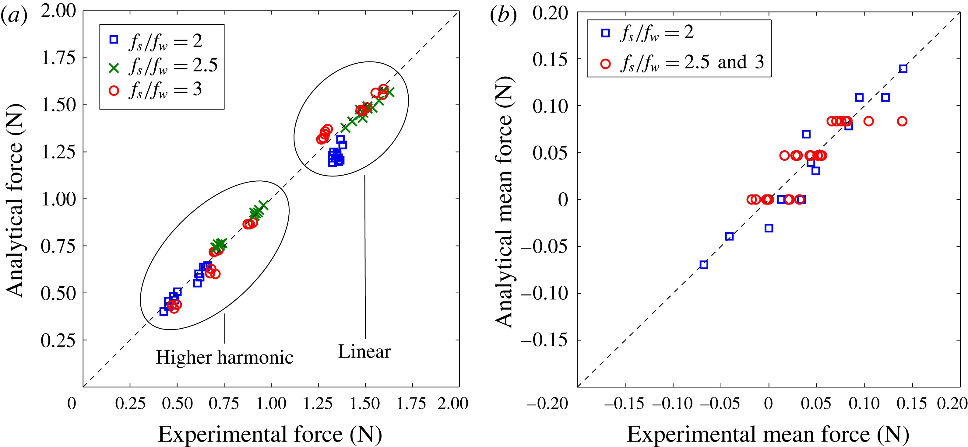
Figure 13 summarises the comparisons between experimental and analytical results for all the asymptotic regimes of
 $u_{c}/u_{w}=1/4-1/3$
in terms of peak values of force harmonics for (a) linear and higher harmonics as well as (b) mean force. The higher harmonic for each
 $f_{s}/f_{w}$
is the component primarily driven by the structural oscillation, which is grouped with adjacent harmonic components as before, but neglecting the next dominant harmonic higher than the structural excitation harmonic. For the linear force comparison, reasonably good agreement is obtained for all
 $f_{s}/f_{w}$
. The data points are homogenously distributed, demonstrating that the linear force component is affected by
 $u_{w}$
more than
 $u_{s}$
and
 $u_{c}$
, as well as the relative phase between
 $u_{w}$
and
 $u_{s}$
. The slight under-prediction for
 $f_{s}/f_{w}=2$
is largely due to a matter of the choice of
 $C_{m}$
in the fitted inertia force, which is in a way similar to the F3B case where
 $C_{m}$
needs to be increased for a better fit. For presentational purposes, such agreement is considered satisfactory. For the higher harmonic comparison, there are two separate clusters of data points due to contributions from two different
 $u_{s}$
(and another two separate clusters for F3A and F3B motions), and relatively good agreement is achieved for all cases.
It should be noted that there are two mean force models in the analytic form as presented in (3.11), and both models agree relatively well with the measured mean forces for all cases. Notice that for the asymptotic flow regime, the mean force is less than
 ${\sim}1/10$
of the main sinusoidal component of the linear force. Hence, given that the mean force is a small fraction of the peak forces within a wave cycle, we view this level of consistency as satisfactory.
Comparison between experimental and analytical results for all the asymptotic regimes of
 $u_{c}/u_{w}=1/4-1/3$
in terms of (a) linear and higher harmonic force, and (b) mean force.

Overall, we have demonstrated the adequacy of the proposed wave–current–structure blockage model presented in (3.11) and (3.12) in reproducing the required force peaks as well as time histories of the force harmonics for all the cases.
4 Discussion
4.1 On the use of numerical modelling
For non-asymptotic flow regimes whereby
 $u_{c}/u_{w}=1/2-1$
, no simple analytical form is available. Moreover, for a more realistic problem involving non-regular free-surface gravity waves with flow kinematics varying with depth, the analytical form is certainly inadequate. Therefore, numerical modelling is a more suitable approach.
Previous studies by Santo et al. (Reference Santo, Taylor, Bai and Choo2014a , Reference Santo, Taylor, Bai and Choo2015, Reference Santo, Stagonas, Buldakov and Taylor2017, Reference Santo, Taylor, Day, Nixon and Choo2018) treated a space-frame structure as a porous block and achieved some success in reproducing the measured peak forces as well as complete force–time histories. Similar work has been conducted on characterising resistance based on drag and Morison equations in related fields: see e.g. Kristiansen & Faltinsen (Reference Kristiansen and Faltinsen2012), Zhao et al. (Reference Zhao, Bi, Dong, Gui, Cui, Guan and Xu2013) and Chen & Christensen (Reference Chen and Christensen2016). Hence, it is of interest to apply the same modelling approach by representing the grids of perforated flat plates as a porous block with the same amount of resistance and added mass (a representation of the equivalent Morison drag and inertia stress terms in the governing Navier–Stokes equations). A similar numerical set-up to the two-dimensional forced oscillation as described in § 5.2 of Santo et al. (Reference Santo, Taylor, Bai and Choo2014a ) is used. The main difference is that now we consider force oscillation at three scales, with an additional structural oscillation which was not considered previously.
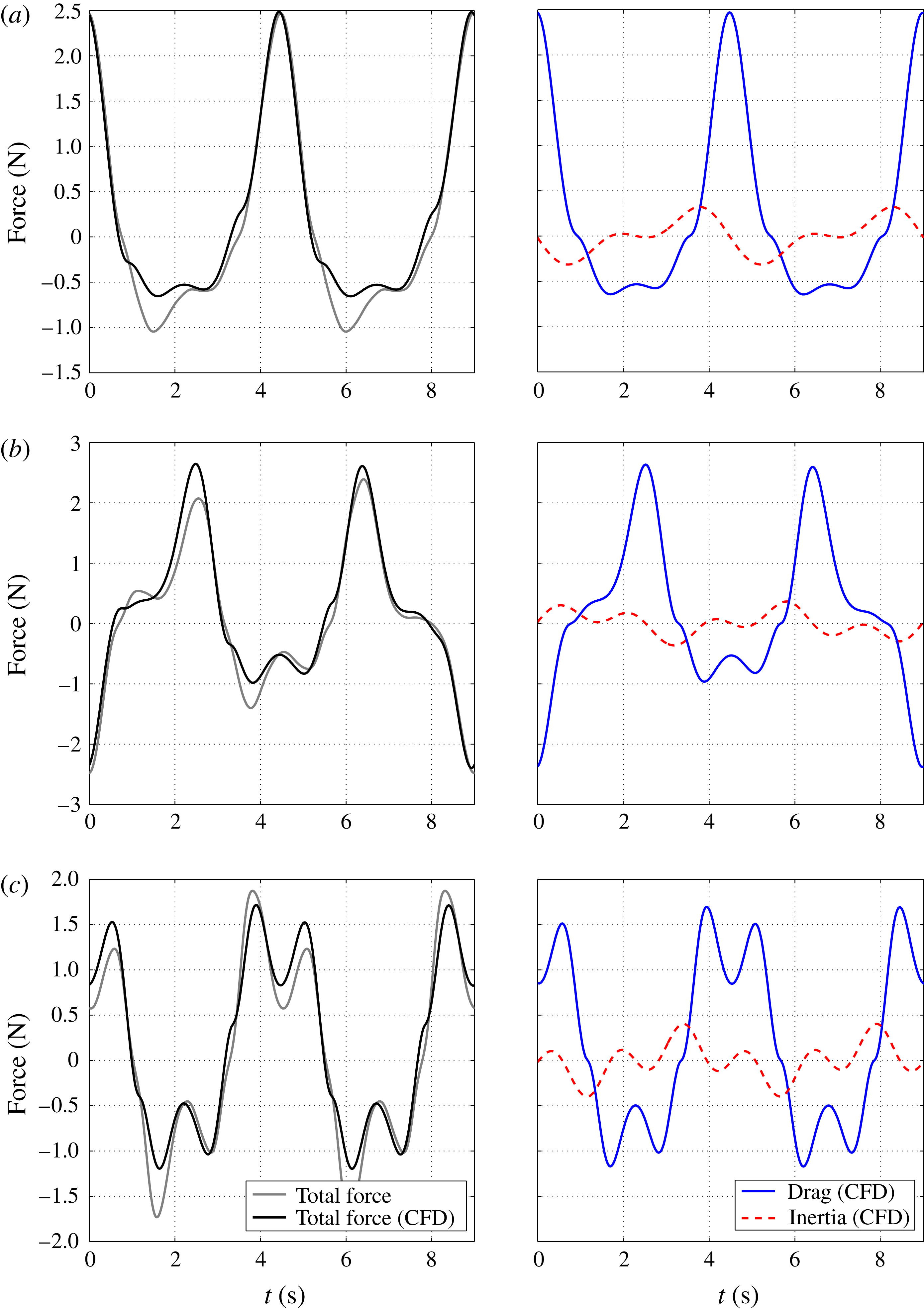
Comparison of total force–time history (left column of each panel) and simulated drag and inertia force–time history (right column of each panel) for three cases of [12, 4, 4]: (a) F2A, (b) F2.5C and (c) F3B.

Figure 14 presents results in terms of total force–time history (left column of each panel) and simulated drag and inertia force–time history (right column of each panel) for three cases of [12, 4, 4]. The comparison between experimental and numerical results is shown in terms of total force–time history only as we are unable to separate the measured drag component from the inertia component without invoking the velocity (and hence drag) symmetry assumption in the force decomposition. Hence, the numerical force–time history is obtained using the best fit of
 $C_{d}$
and
 $C_{m}$
from table 4 in each of the numerical simulations. Relatively good agreement is obtained in general, although the mean force of the numerical total force is observed to be larger, such that the trough (or the crest) of the total force is under-predicted (or over-predicted) relative to the measured total force.
The simulated inertia force exhibits smooth variation with a clear separation of two time scales (wave and structural acceleration). Since inertia force components are associated with potential-flow-type distortions, the inertia force is only marginally affected by wake-related features, hence the inertia force is smoother and symmetric in time relative to drag force. Moreover, the simulated inertia force compares relatively well with the analytical Morison inertia prediction according to (3.11).
The numerical drag force exhibits slight asymmetry in time when there is the ‘plateau’ in the imposed velocity (hence acceleration is
 ${\sim}$
zero). However, the asymmetry in the measured drag force and hence the total force is more pronounced, which explains some of the discrepancies in the total force–time history comparison. As previously discussed in § 3.2, the drag asymmetry can probably be associated with wake-related flow structures which in turn are related to the physical grids of perforated plates. Since these grids are smeared out into a single porous block in the numerical model, only the global flow features (global wake effect) which scale as the frontal width of the grid are captured. The slight asymmetry from the numerical drag force is thus due to biasing from the mean flow associated with the large-scale flow structures only. By comparing to the measured force results with a more pronounced force asymmetry, we speculate that the difference might be attributed to additional contribution from local fine-scale structures (such as vortex shedding) which scale as individual bar width, and these are not represented in the numerical modelling.
4.2 On the scale effects
Although the series of laboratory-scale experiments is carefully designed and conducted to assist understanding of fluid loading at a fundamental level, it inevitably suffers from scale effects. The laboratory-scale results are affected by the low Reynolds number, lower by a factor 100–1000 than applications to offshore structures. In particular, the
 $C_{d}$
coefficient will be affected by the different turbulent flow regimes. Therefore, we do not expect the same fitted
 $C_{d}$
values could be used for larger Reynolds number. Using the same fluid loading model accounting for wave–current blockage, Santo et al. (Reference Santo, Taylor, Day, Nixon and Choo2018) observed that
 $C_{d}=1$
–1.3 is appropriate for a larger scale of offshore jacket model comprising multiple cylinders, in contrast to the flat bar obstacles used here.
Note that since no free-surface fluctuation is used in the experiments to represent gravity waves, there is no dependency on Froude number.
4.3 On the comparison with the present industry practice
Present industry practice in assessing the hydrodynamic force on dynamically responding space-frame offshore structures is to use the standard Morison equation with a reduced current velocity according to Taylor (Reference Taylor1991) (see for example American Petroleum Institute 2000) and with the relative-velocity formulation. The force model for the present industry practice is as shown in (3.1), and to account for current blockage effect, the free-stream current velocity
 $u_{c}$
is reduced to the shielded current velocity
 $u_{cs}$
, with
 $u_{cs}=u_{c}/(1+(C_{d}A)/(4A_{f}))$
.
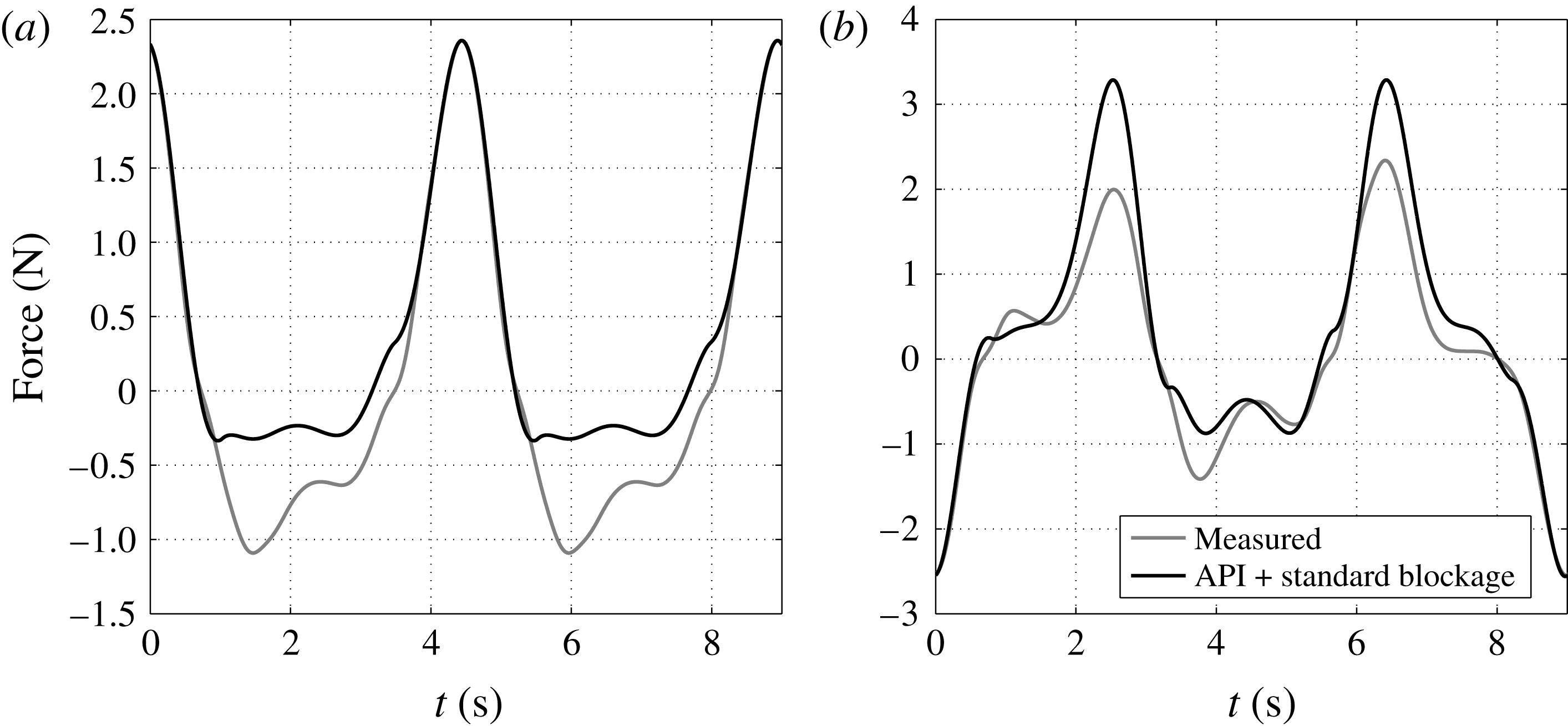
Comparisons between the present industry model and our measurements are shown in figure 15 for two particular cases of [12, 3, 4]. It is obvious from the comparison that the present industry model can only match the measured peak force using a smaller but time-invariant
 $C_{d}$
but not the entire measured force–time history, and this applies to all other cases as well (the American Petroleum Institute (API) model is matched at time
 $=0$
for both cases). Since a correct representation of the entire force–time history is essential for a dynamically responding structure, a time-variant
 $C_{d}$
would be required. This illustrates the inadequacy of present industry practice in representing the actual hydrodynamic force on a space-frame structures. The wave–current–structure blockage model, which has been validated in § 3, in parallel with the use of numerical modelling using a porous block approach, is proposed as a better alternative.
Comparison of total force–time history between measurement (grey lines) and fitted force using API with standard blockage (solid lines) for two cases of [12, 3, 4]: (a) F2A, and (b) F2.5C.

5 Conclusions
In this series of experiments, three grids of perforated flat plates are moved with three scales of motion in otherwise still water and the associated hydrodynamic forces are recorded for a range of motion combinations. For a real offshore structure, this represents a steady current (
 $u_{c}$
), the low frequency and high amplitude fluid motion driven by incident waves (
 $u_{w}$
) and the high frequency but small amplitude dynamic motion of the structure (
 $u_{s}$
). Building on the previous wave–current blockage model by Santo et al. (Reference Santo, Taylor, Williamson and Choo2014b
), a new wave–current–structure blockage model is developed based on the Morison equation with the relative-velocity formulation. For an asymptotic flow regime of
 $u_{w}\gg u_{c}$
, the drag force component of the new model is consistent with that of the previous wave–current blockage model, except with an additional
 $u_{s}$
contribution into both the wave drag and the current drag components. The inertia force component can be expressed as a summation of the potential-flow-type perturbations due to oscillatory wave and structural motions with a single Morison inertia coefficient. The analytical model, which requires only a calibration of the Morison type drag and inertia coefficients, is compared with the measured forces. Reasonably good agreement is achieved not only in terms of peak forces and complete force–time histories, but also in terms of force harmonic components ranging from a rather small mean force, the dominant linear frequency component driven by the wave oscillation, to the higher harmonic component primarily driven by the structural oscillation.
For some of the motion combinations, biasing by the mean flow induces obvious (drag) force asymmetry in the measured total force. Hence, it is not possible to decompose the total force using the method introduced by Santo et al. (Reference Santo, Taylor, Williamson and Choo2014b ) which assumes drag force symmetry. The comparison between analytical prediction and measurement is thus performed based on total force. When there is drag force asymmetry, there is a shift on the drag force shoulders (inflexion points) around zero crossings, but the peak forces remained unchanged. The force asymmetry can be accounted for artificially by introducing a phase shift to the higher force harmonic driven by the structural oscillation. The analytical model is shown to reproduce relatively well all the measured total force–time histories, regardless of whether a phase shift or zero phase shift is imposed on the higher harmonic component of the fitted drag term. Using the present industry practice, however, the predicted force can only be fitted at a single instant of the oscillation cycle using the best fit of Morison drag and inertia coefficients, but nowhere else along the entire force–time history, demonstrating the serious inadequacy of the present recipe.
Numerical simulation is conducted using a porous block as a numerical model of the grids. The simulated inertia force is found to vary smoothly with two periodic time scales, consistent with the inertia force predicted by the analytical model. The simulated drag force is observed to contain force asymmetry, although only slight, which is due to biasing from the mean flow associated with large-scale flow structures. Hence, the more pronounced drag force asymmetry observed experimentally must be related to local fine-scale flow structures which scale as the individual bar width and are not represented numerically. The application of the porous block approach to this scale of experiment clearly has some limitations.
Overall, this paper demonstrates the adequacy of the concept of relative flow fields (relative-velocity formulation) in the Morison equation to account for the additional high frequency structural motion as well as the validity of the extended analytical Morison-based blockage model to capture the wave–current–structure blockage effects.
Acknowledgements
We gratefully acknowledge the enthusiastic help and contributions made by the team members of Charles H. K. Williamson Laboratory of Cornell University, especially D. Asselin, S. Morris and J. Young. We would also like to acknowledge the support from the Singapore Maritime Institute (SMI) through grant no. SMI-2015-AIMP-030.
Appendix A. Data correction due to gravity
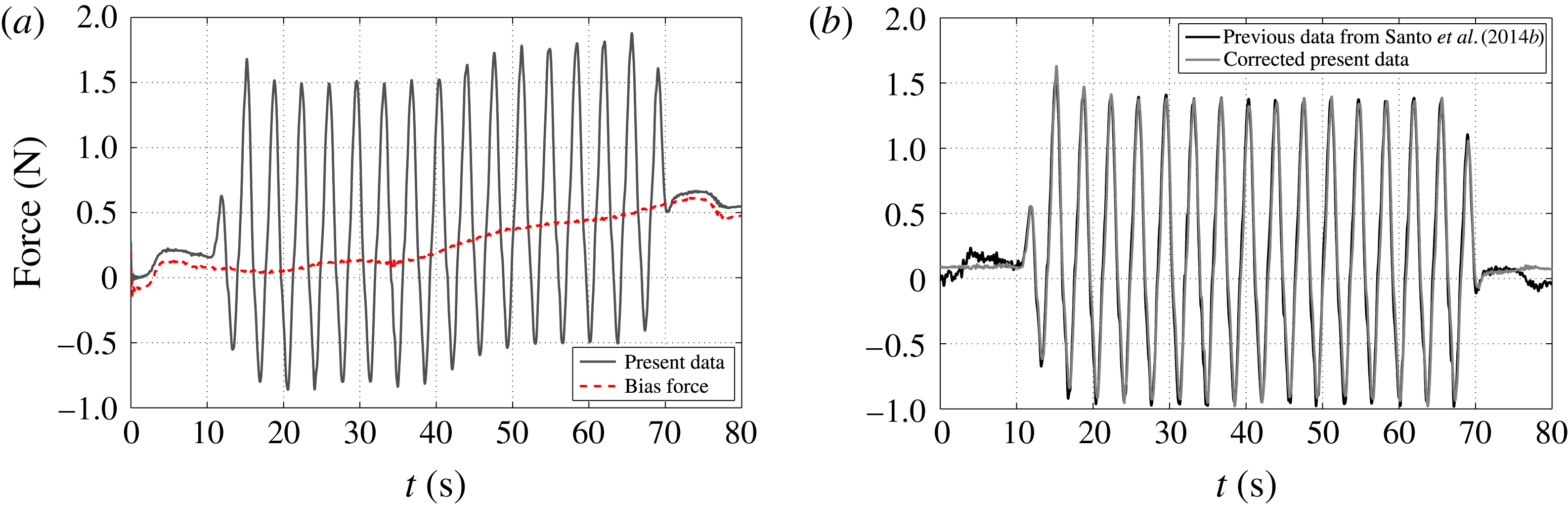
All the recorded total force signals in the present experiment contain a bias due to a set-up error for the XY towing tank in a newly refurbished laboratory: the rails along the sides of the tank were not quite level. The resulting bias signal is essentially a small component of gravity acting along the tank, which is picked up by the force transducer.
The force bias at each location of the tank within the zone of interest could have been measured by recording the voltage when the grid and water were stationary, and the sloping force as a function of location could have been deduced from there. What was done instead is a force measurement of steady tow from one point to another covering the zone of interest. It is thus possible to compare the force measurement for steady tow between the present and the previous tests by Santo et al. (Reference Santo, Taylor, Williamson and Choo2014b
) under the same towing speed (
 $u_{c}$
). With the assumption that the true measured fluid force is unchanged, one can deduce the bias force due to gravity as a function of position, which can then be used to correct the measured total force of each case. Figure 16 gives an example of the measured total force before and after the correction.
(a) Measured total force and gravity force as a function of time. (b) The corrected measured total force plotted with the result from the previous experiments conducted by Santo et al. (Reference Santo, Taylor, Williamson and Choo2014b
) for the same [
 $u_{w}$
,
 $u_{c}$
] and grid configuration.

Appendix B. Table of inferred
 $C_{d}$
and
$C_{m}$


Inferred Morison coefficients.