1 Introduction
The character of turbulent structures, their evolution and how they are distributed in a turbulent flow are of great importance to understand their dynamics and to drive their modelling. Lagrangian dynamics offers a possibility to investigate that. In contrast to Eulerian dynamics, Lagrangian dynamics describes a flow in a reference system that is fixed with a fluid particle, instead of an inertial system which is fixed with the flow domain. This allows a different perspective on the flow. However, most flow simulations, including the present direct numerical simulation (DNS), rely on an Eulerian description of the considered system. In order to exploit data from an Eulerian system in the Lagrangian dynamics analysis, the velocity-gradient tensor invariants are possible connections, as they are invariant by rotation or translation. Furthermore, the velocity-gradient tensor contains rich information about the flow and its dynamics. For instance, Perry & Chong (Reference Perry and Chong1987) summarized how local flow patterns can be characterized by the velocity-gradient tensor at the locations of interest. From the point of view of a fluid particle located in a structure, it allows the distinction between four different states of the structure at the location of the particle. In detail, for incompressible or weakly compressible flow, in which
 $P$
defined in (3.2a
) equals or is close to zero, the space spanned by
 $Q$
and
 $R$
defined in (3.2b
) and (3.2c
), respectively, can be divided into four sectors by the
 $\unicode[STIX]{x1D6E5}=0$
line and
 $R=0$
line, where
 $\unicode[STIX]{x1D6E5}$
is the discriminant of the velocity-gradient tensor matrix. These four sectors correspond to four characteristic structure types: (
 $S$
I) vortical structures with stretching character (
 $\unicode[STIX]{x1D6E5}>0,~R\leqslant 0$
); (
 $S$
II) vortical structures with contracting character (
 $\unicode[STIX]{x1D6E5}>0,~R>0$
); (
 $S$
III) pure straining structures with flattening character (
 $\unicode[STIX]{x1D6E5}\leqslant 0,~R>0$
); and (
 $S$
IV) pure straining structures with elongating character (
 $\unicode[STIX]{x1D6E5}\leqslant 0,~R\leqslant 0$
). Sketches of these topologies can be found in Ooi et al. (Reference Ooi, Martin, Soria and Chong1999). A review by Meneveau (Reference Meneveau2011) summarized most of the progress achieved in the field of Lagrangian dynamics of the velocity-gradient tensor. More detailed explanations of the structure types can also be found in Perry & Chong (Reference Perry and Chong1987) and Bechlars (Reference Bechlars2015), for example. For compressible turbulence, two more sectors will appear in the
 $QR$
space for a given
 $P$
value. Detailed explanations on the flow behaviour for these additional sectors and the characteristics of cases at relatively higher or extreme
 $P$
values (both positive and negative values) from DNS results for decaying compressible isotropic turbulence can be found in Suman & Girimaji (Reference Suman and Girimaji2010).
The joint probability density function (joint p.d.f.) of
 $Q$
and
 $R$
(or the
 $QR$
plot) can statistically describe the characteristic composition of turbulence for targeted regions. The isolines of this joint p.d.f. for many flows have similar shape, reminiscent of a teardrop (Soria et al.
Reference Soria, Sondergaard, Cantwell, Chong and Perry1994; Chong et al.
Reference Chong, Soria, Perry, Chacin, Cantwell and Na1998; Ooi et al.
Reference Ooi, Martin, Soria and Chong1999). However, variations of this
 $QR$
plot shape have been found for different flows, especially for wall-bounded flows, which have a wide range of practical applications and are important to be understood. For instance, from DNS of wall-bounded flows, it has been found that the shapes of the
 $QR$
plot at the outer-layer locations of the boundary layer has the teardrop shape, whereas in the buffer layer the tail of the
 $QR$
plot shrinks compared to locations further away from the wall. This difference has been found both from channel flows (Blackburn, Mansour & Cantwell Reference Blackburn, Mansour and Cantwell1996) and from turbulent boundary layer flows (Chacín, Cantwell & Kline Reference Chacín, Cantwell and Kline1996; Wang & Lu Reference Wang and Lu2012). Most recently, the considerable change of the
 $QR$
evolution for different wall-normal locations has been studied and the wall effects have been discussed by Bechlars & Sandberg (Reference Bechlars and Sandberg2017a
,Reference Bechlars and Sandberg
b
) for a zero-pressure-gradient (ZPG) turbulent boundary layer at a free-stream Mach number of 0.5. The smooth changes in the outer layers were contrasted by the strong variations in the near-wall region.
However, although a significant amount of research involving the
 $QR$
analysis has been devoted to ZPG boundary layers, the same cannot be said for boundary layer flows with pressure-gradient effects. These flows are usually found around surfaces with curvature, as encountered in many aerodynamic applications such as aerofoils, wings and blades, which have significant engineering importance. The literature (Lee & Sung Reference Lee and Sung2009; Gungor et al.
Reference Gungor, Maciel, Simens and Soria2014; Yuan & Piomelli Reference Yuan and Piomelli2015) reveals that, for subsonic boundary layers that are subject to a favourable pressure gradient (FPG) or an adverse pressure gradient (APG), the flow topology and the mean statistics show significant changes compared with ZPG turbulent boundary layers as a result of flow acceleration and deceleration. For FPG boundary layers, the flow accelerates and the relaminarization – or, more accurately, quasi-laminarization (Yuan & Piomelli Reference Yuan and Piomelli2015) – is often observed when the FPG is strong enough. The turbulence kinetic energy (TKE), however, of the mean flow continues to increase as a result of the acceleration, yet the flow may become less dynamic. Narasimha & Sreenivasan (Reference Narasimha and Sreenivasan1973) attribute this phenomenon to the dominance of pressure forces over the slowly responding Reynolds stresses. From a flow structure point of view, Bourassa & Thomas (Reference Bourassa and Thomas2009) showed that the quasi-laminarization is related to the stabilizing effects of the acceleration on near-wall streaks caused by the decrease of the wall-normal and spanwise fluctuations. Recently, Piomelli & Yuan (Reference Piomelli and Yuan2013) further extended this conclusion with the help of a large-eddy simulation (LES), stating that the decrease of the wall-normal and spanwise fluctuations is caused by the decrease of the magnitude of the pressure fluctuations, from a source term of the Poisson equation, which points to a redistribution of the TKE which finally leads to quasi-one-dimensional turbulence in the quasi-laminarization zones. For APG boundary layers, the flow decelerates and the boundary layer becomes thicker, and if the APG is strong enough, the flow separates from the wall. It was reported that the velocity profiles of APG flows do not follow the classical law of the wall (Von Kármán Reference von Kármán1931), even very close to the wall (Afzal Reference Afzal1983; Nagano, Tsuji & Houra Reference Nagano, Tsuji and Houra1998; Indinger, Buschmann & Gad-el Hak Reference Indinger, Buschmann and Gad-el Hak2006; Lee & Sung Reference Lee and Sung2008; Gungor et al.
Reference Gungor, Maciel, Simens and Soria2014). Lee & Sung (Reference Lee and Sung2008) show that the energy redistribution is enhanced in the outer layer of the APG flows compared to the ZPG flow using data from an incompressible flow DNS. Later Gungor et al. (Reference Gungor, Maciel, Simens and Soria2014) performed DNS of a turbulent boundary layer exposed to a strong APG and found that the mean velocity profiles do not reveal a logarithmic law and Reynolds stress peaks move to roughly the middle of the boundary layer. From a modelling point of view, turbulent flows with an APG have been regarded as being among the most difficult flows to predict using turbulence models (Wilcox Reference Wilcox1998). DNS can provide accurate information directly. To specify proper boundary conditions that result in a specific pressure distribution is vital, especially if the simulated flow is to be compared with experiments. This provides the original motivation of the current work: to produce a reliable database of a turbulent boundary layer subject to pressure gradients that can be studied to gain a deeper understanding of the effect of pressure gradients on the turbulence dynamics. Also, most of the previous studies on turbulent flows with pressure-gradient effects mentioned above have limited themselves to discussions of mean profiles, while the
 $QR$
analysis can give new perspectives to such flows, which, to the authors’ knowledge, has never been reported before.
In the present work, a particular emphasis is put on the
 $QR$
evolution caused by pressure gradients for different wall-normal locations throughout the turbulent boundary layer over a curved surface. The compressible flow DNS of a controlled-diffusion (CD) aerofoil that was carried out by Wu et al. (Reference Wu, Sanjosé, Moreau and Sandberg2018) to provide the necessary dataset is outlined in § 2. In § 3 the compressible evolution system for the first three invariants of the velocity-gradient tensor is briefly presented. The results of the analysis are shown in § 4 with discussions on the differences in the investigated regions. The mean flow profiles under different pressure-gradient conditions are firstly presented in § 4.1; then the resulting mean evolution at different locations in the boundary layer is shown in § 4.2 and the contributions of its separate components are shown in § 4.3. Wall effects are discussed in § 4.4. Conclusions are drawn in § 5.
2 Flow data over a controlled-diffusion aerofoil
A three-dimensional (3D) compressible DNS is conducted of the flow over a CD aerofoil at 8
 $^{\circ }$
geometrical angle of attack that is embedded in the jet potential core of a free-jet wind tunnel at an aerofoil chord-based Reynolds number of
 $Re_{c}=150\,000$
and at a Mach number of
 $M=0.25$
. Such a profile is representative of many modern industrial applications, including low-pressure compressors, a turbofan at approach, and aerospace or automotive ventilation systems. The volume data around the aerofoil and the near wake were recorded during the simulation at a sampling frequency of 78 kHz for five flow-through times based on the reference velocity and aerofoil chord length, once the simulation was statistically steady. For this flow case (Moreau et al.
Reference Moreau, Henner, Iaccarino, Wang and Roger2003; Moreau & Roger Reference Moreau and Roger2005; Wang et al.
Reference Wang, Moreau, Iaccarino and Roger2009), a short separation bubble is formed at the aerofoil leading edge (LE) on the suction side which triggers the laminar to turbulent transition of the flow. After the transition, the flow remains turbulent and attached and firstly encounters an FPG, then a ZPG around mid-chord and finally an APG in the trailing-edge (TE) area due to the aerofoil camber. On the pressure side, the flow stays laminar until the TE where minor vortex shedding originates due to the blunt (round) TE and then mixes with the turbulent flow from the suction side in the near wake. The present work concentrates on the turbulent flow on the suction side after transition.
2.1 Numerical set-up
The volume data around the aerofoil and the near wake are obtained from a multi-block structured high-order-accurate compressible Navier–Stokes DNS code (Sandberg Reference Sandberg2015). A five-point fourth-order central standard-difference scheme with Carpenter boundary stencils (Carpenter, Nordström & Gottlieb Reference Carpenter, Nordström and Gottlieb1999) is applied for the spatial discretization in the streamwise and crosswise directions. A spectral method using the FFTW3 library is used in the spanwise direction. Time marching is achieved by an ultra-low-storage five-step fourth-order Runge–Kutta scheme (Kennedy, Carpenter & Lewis Reference Kennedy, Carpenter and Lewis1999) with a constant time step of
 $\unicode[STIX]{x0394}t=7.5\times 10^{-6}$
. Unphysical numerical reflections at the computational boundaries are avoided by the choice of appropriate boundary conditions. Characteristic-based boundary conditions (Kim & Lee Reference Kim and Lee2003; Sandberg & Sandham Reference Sandberg and Sandham2006; Jones, Sandberg & Sandham Reference Jones, Sandberg and Sandham2008) are used for this simulation on domain boundaries (for more details, see Wu et al. (Reference Wu, Sanjosé, Moreau and Sandberg2018)). At the aerofoil surface, an adiabatic, no-slip condition is applied. The computational domain comprises six blocks. Specifically, the aerofoil is surrounded by an O-type grid due to the round leading and trailing edges, and the grid refinement in the boundary layers is guided by data obtained from experiments (Moreau et al.
Reference Moreau, Henner, Iaccarino, Wang and Roger2003; Wu et al.
Reference Wu, Laffay, Idier, Jaiswal, Sanjosé and Moreau2016). In the spanwise direction, 96 Fourier modes are employed with 100 % dealiasing, which corresponds to 194 collocation points in physical space. This number of points was found to be sufficient to resolve down to the Kolmogorov scale for a similar flow case (Winkler, Sandberg & Moreau Reference Winkler, Sandberg and Moreau2012) and the current case (Wu et al.
Reference Wu, Sanjosé, Moreau and Sandberg2018) using the same code. These points are distributed over a spanwise width
 $L_{z}$
of
 $0.12c$
(chord length
 $c=0.1356$
m), which has been shown to be enough to get fully decorrelated turbulence in the span (Moreau & Roger Reference Moreau and Roger2005; Wang et al.
Reference Wang, Moreau, Iaccarino and Roger2009; Wu et al.
Reference Wu, Sanjosé, Moreau and Sandberg2018). The grid transition from TE to near wake is achieved to yield a maximum skewness smaller than 0.2. In the wake region, the refinement is centred along the wake deviation line which is known from velocity profiles by hot-wire (HW) measurements and particle image velocimetry (PIV) measurements (Moreau, Neal & Foss Reference Moreau, Neal and Foss2006; Neal Reference Neal2010). The total grid size is 345 million, in which the O-grid around the boundary layer comprises
 $3341\times 279\times 194$
grid points.
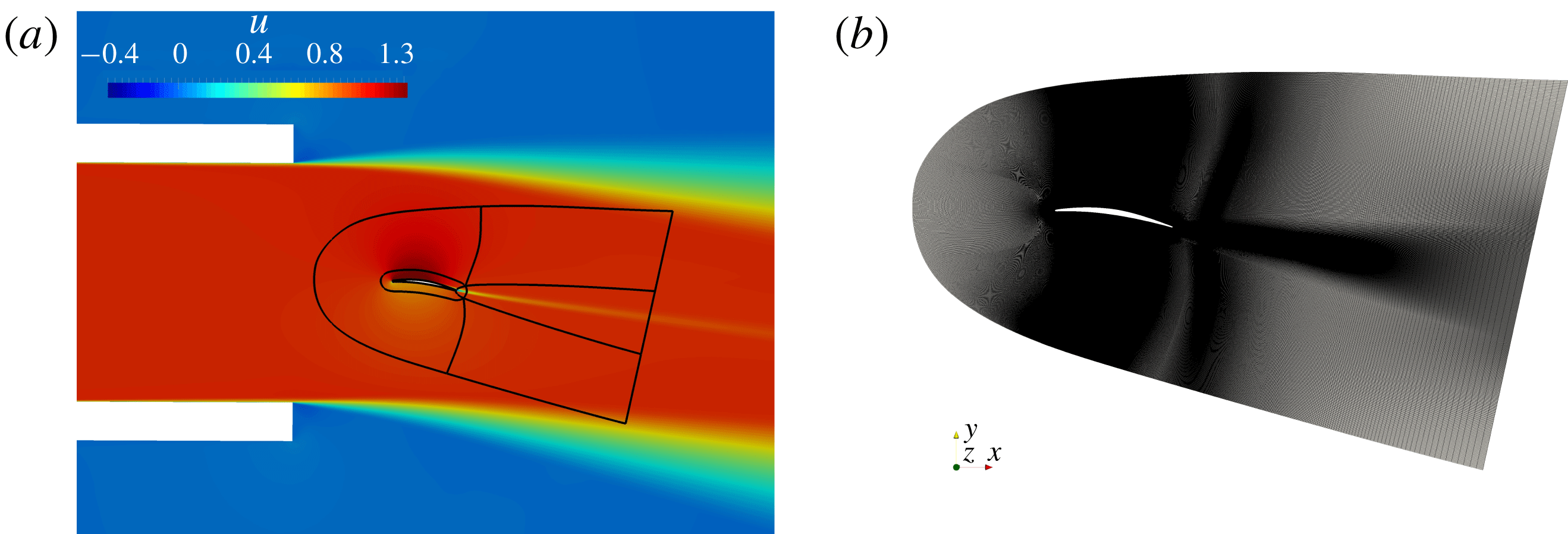
(a) Grid topology of the wind-tunnel set-up for initial RANS computations together with the DNS domain outlines (black lines). (b) Truncated domain for DNS set-up.

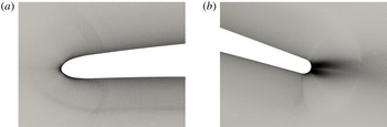
DNS mesh details: (a) LE; (b) TE and near wake.

In order to properly reproduce the experimental set-up for this flow case, installation effects (Moreau et al. Reference Moreau, Henner, Iaccarino, Wang and Roger2003), mainly the effects of the jet on aerofoil loading, have to be considered. To account for such effects, one possible approach is to include both the jet and aerofoil in the simulation. This would, however, make the DNS computationally very expensive, if not impossible, with current resources. In order to remedy this, an efficient procedure has been implemented to include wind-tunnel installation effects in the numerical set-up of an unsteady simulation (Christophe, Anthoine & Moreau Reference Christophe, Anthoine and Moreau2008, Reference Christophe, Anthoine and Moreau2009; Wang et al. Reference Wang, Moreau, Iaccarino and Roger2009; Christophe Reference Christophe2011). For the current flow case, firstly a two-dimensional (2D) Reynolds-averaged Navier–Stokes (RANS) computation of the flow around the aerofoil was conducted, taking into account the complete nozzle shape and geometrical configuration that were used in the experiments. Considering the low Mach number in the experiments, incompressible flow solutions were used in both RANS and LES. The nozzle outlet velocity profile was known from HW measurements and these velocity data were used to define the steady inflow conditions to the RANS domain.
The
 $k{-}\unicode[STIX]{x1D714}$
shear stress transport (SST) model was found to predict better global behaviour considering the velocity and TKE profiles when the results are systematically compared with experimental data (Moreau et al.
Reference Moreau, Henner, Iaccarino, Wang and Roger2003; Wu et al.
Reference Wu, Laffay, Idier, Jaiswal, Sanjosé and Moreau2016). In a second step, a truncated domain comprising six blocks as shown by the black lines in figure 1(a) was used for the DNS solver. The initial field in the DNS is directly interpolated from the RANS solution onto the DNS grid as shown in figure 1(b). Figures 2(a) and 2(b) show magnified images of the grid near the LE and the TE, respectively. The velocity profiles for the inlets of the DNS domain come from the RANS that mimic the influence of the wind tunnel on the flow field around the aerofoil. In particular, it accounts for the mean effects of flow deflection. As also mentioned by Deniau et al. (Reference Deniau, Dufour, Boussuge, Polacsek and Moreau2011) using a similar procedure for a first compressible LES on a NACA651210 aerofoil, it should be noted that the truncated DNS domain boundaries are placed so that: firstly, these boundaries do not touch the shear layer from the wind-tunnel exit to exclude extra computational efforts to resolve these shear layers; secondly, the velocity vectors from RANS are checked so that these vectors are real inlets to the DNS domain to avoid possible recirculations or outflow for those boundaries in the DNS; and thirdly, these domain boundaries should be far enough from the aerofoil to allow the boundary condition to damp both turbulent structures and acoustic waves efficiently to avoid possible spurious reflections.
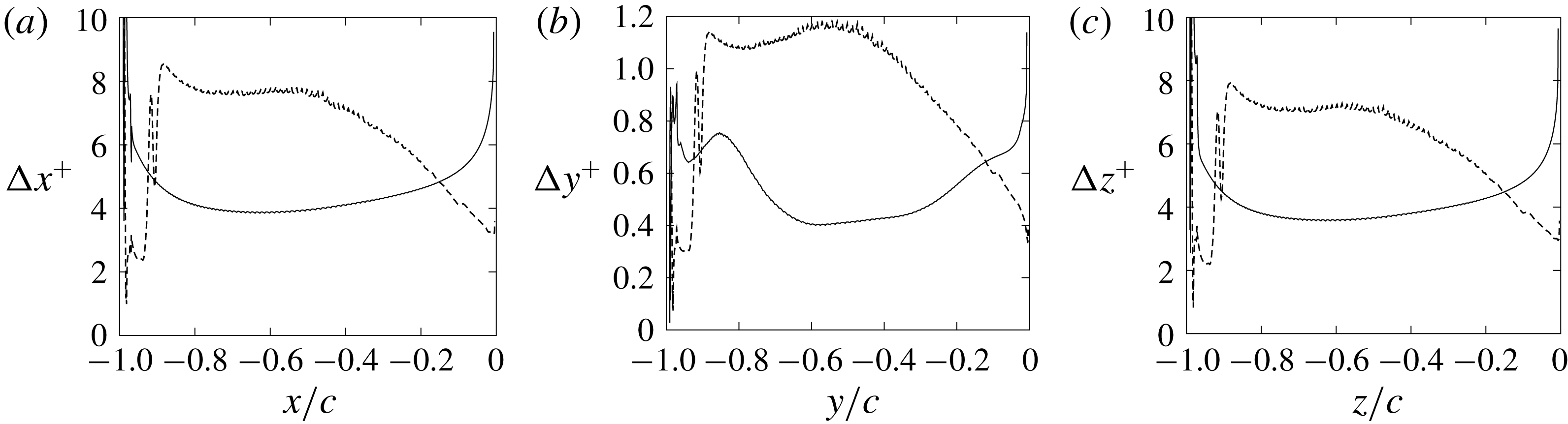
DNS grid resolution around the CD aerofoil (– – – –, suction side; ——, pressure side) (Wu et al. Reference Wu, Sanjosé, Moreau and Sandberg2018).

2.2 Validation and flow topology
Firstly, as shown in figure 3, the grid resolution around the aerofoil has been checked by looking at the dimensionless grid size based on the friction velocity
 $u_{\unicode[STIX]{x1D70F}}$
. The maximum values are
 $\unicode[STIX]{x0394}x_{max}^{+}\approx 8.5$
,
 $\unicode[STIX]{x0394}y_{max}^{+}\approx 1.2$
and
 $\unicode[STIX]{x0394}z_{max}^{+}\approx 7.9$
. These values compare well with the reference aerofoil DNS cases (Jones et al.
Reference Jones, Sandberg and Sandham2008) using the same code in the regions of interest where turbulent flows are present and the
 $\unicode[STIX]{x0394}y^{+}$
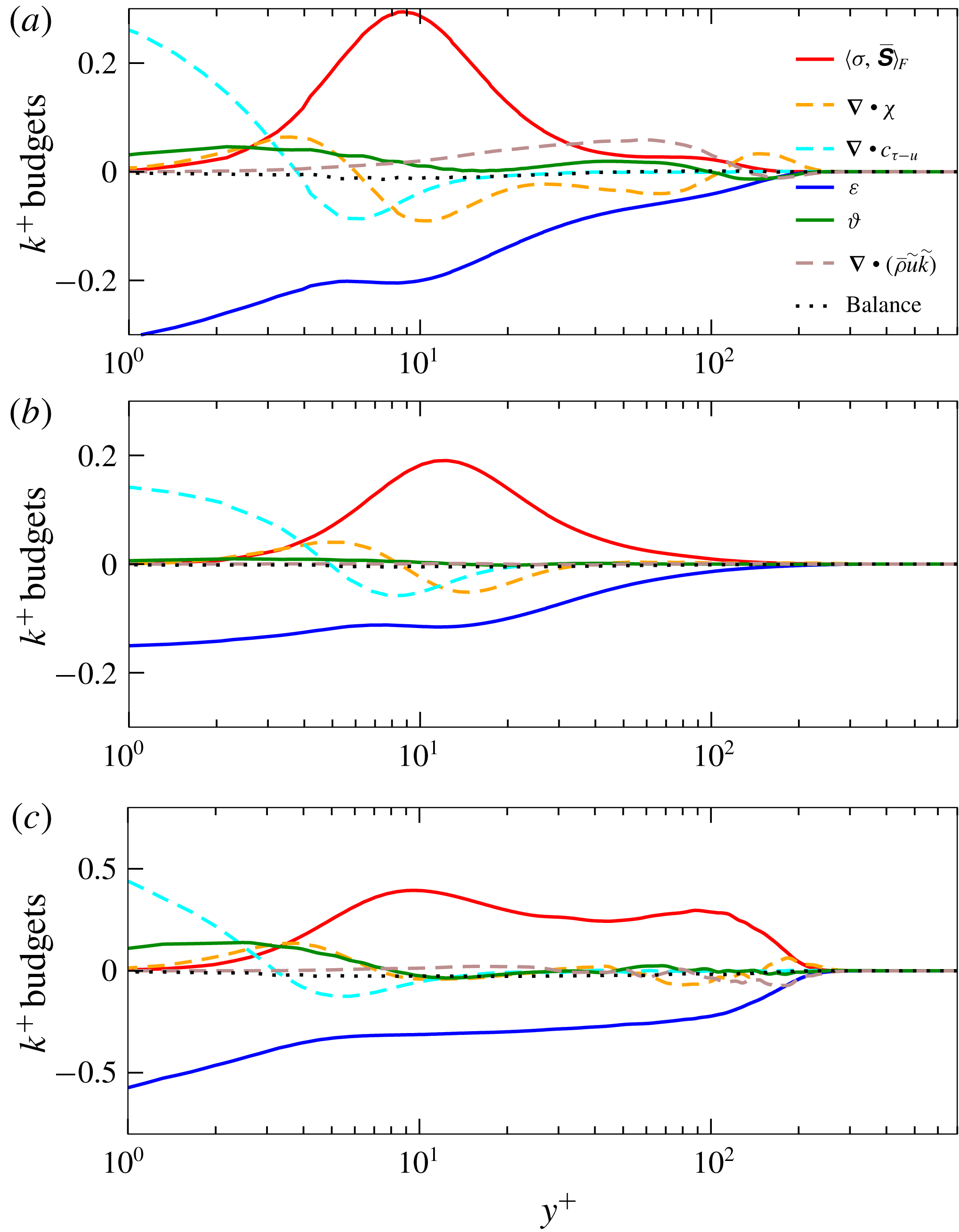
values decrease along the chord and are even better around the aerofoil TE. Furthermore, the mean wall-normal profiles of the TKE budgets are shown together with the balance value in figure 4. The terms of the energy budgets are normalized by a density-weighted factor of
 $Re_{\infty }\unicode[STIX]{x1D70C}^{2}u_{\unicode[STIX]{x1D70F}}^{4}/T$
, to yield
 $k^{+}$
, where
 $T$
is the temperature. The terms of the TKE budgets in figure 4 are defined as:
 $$\begin{eqnarray}\displaystyle \displaystyle \langle \unicode[STIX]{x1D70E},\overline{\unicode[STIX]{x1D64E}}\rangle _{F}:=\text{trace}(\unicode[STIX]{x1D70E}\overline{\unicode[STIX]{x1D64E}}) & & \displaystyle \quad (\text{turbulence production}),\end{eqnarray}$$
 $$\begin{eqnarray}\displaystyle \displaystyle \unicode[STIX]{x1D735}\boldsymbol{\cdot }\unicode[STIX]{x1D74C}:=\frac{\unicode[STIX]{x1D735}\boldsymbol{\cdot }\overline{(\unicode[STIX]{x1D70C}\boldsymbol{u}^{\prime \prime }{\boldsymbol{u}^{\prime \prime }}^{2})}}{2} & & \displaystyle \quad (\text{triple momentum transport}),\end{eqnarray}$$
 $$\begin{eqnarray}\displaystyle \displaystyle \unicode[STIX]{x1D735}\boldsymbol{\cdot }\boldsymbol{c}_{\unicode[STIX]{x1D749}-\boldsymbol{u}}:=\unicode[STIX]{x1D735}\boldsymbol{\cdot }\overline{\unicode[STIX]{x1D749}^{\prime \prime }\boldsymbol{\cdot }\boldsymbol{u}^{\prime \prime }} & & \displaystyle \quad (\text{viscous transport}),\end{eqnarray}$$
 $$\begin{eqnarray}\displaystyle \displaystyle \unicode[STIX]{x1D700}:=\overline{\text{trace}(\unicode[STIX]{x1D749}^{\prime \prime }(\unicode[STIX]{x1D735}\boldsymbol{u}^{\prime \prime })^{\text{T}})} & & \displaystyle \quad (\text{dissipation}),\end{eqnarray}$$
 $$\begin{eqnarray}\displaystyle \displaystyle \unicode[STIX]{x1D717}:=\overline{\boldsymbol{u}^{\prime \prime }\boldsymbol{\cdot }\unicode[STIX]{x1D735}p^{\prime }} & & \displaystyle \quad (\text{pressure transport}).\end{eqnarray}$$
 $\unicode[STIX]{x1D70E}$
and
 $\unicode[STIX]{x1D749}$
denote the Favre stress and viscous stress tensor, respectively,
 $\unicode[STIX]{x1D64E}$
is the strain-rate tensor,
 $\widetilde{\bullet }$
stands for density-averaged Favre-averaged terms,
 $\bullet ^{\prime \prime }$
for the fluctuation around Favre-averaged quantities and the overline represents the mean value in time. The three chosen locations are at 18 %, 40 % and 92 % of the aerofoil chord, which are located in the FPG, ZPG and APG zones, respectively. In general, the turbulence production and dissipation terms are the dominant terms which drive the TKE distribution, except for in the vicinity of the wall. Yet, the differences between zones subject to different pressure-gradient conditions are striking. The FPG zone generally has a similar behaviour to the ZPG zone in the near-wall region but the budget terms have a more complex distribution near the outer layer. The profiles from the ZPG zone for this flow case bear a great resemblance to that from the ZPG turbulent boundary layer of Bechlars & Sandberg (Reference Bechlars and Sandberg2017a
,Reference Bechlars and Sandberg
b
) with a higher Mach number. The APG zone has greater values of the production and dissipation terms compared to the FPG and ZPG zones and the production shows a hump connected by two peak values from the viscous sublayer to the log layer and even to the edge of the outer layer. As the turbulent mixing dynamics mainly stems from these two factors, this indicates that the APG helps enhance this mixing. The balance value, which is the sum of the TKE budget terms, is very close to 0 (maximum absolute value approximately 0.004) for all locations which indicates that the current DNS correctly resolves the dissipation range for those investigated regions across the boundary layer and the statistical averaging time is sufficiently long for these statistics that are up to third order.
Wall-normal profiles of TKE budgets: (a) FPG, (b) ZPG zones and (c) APG zones.

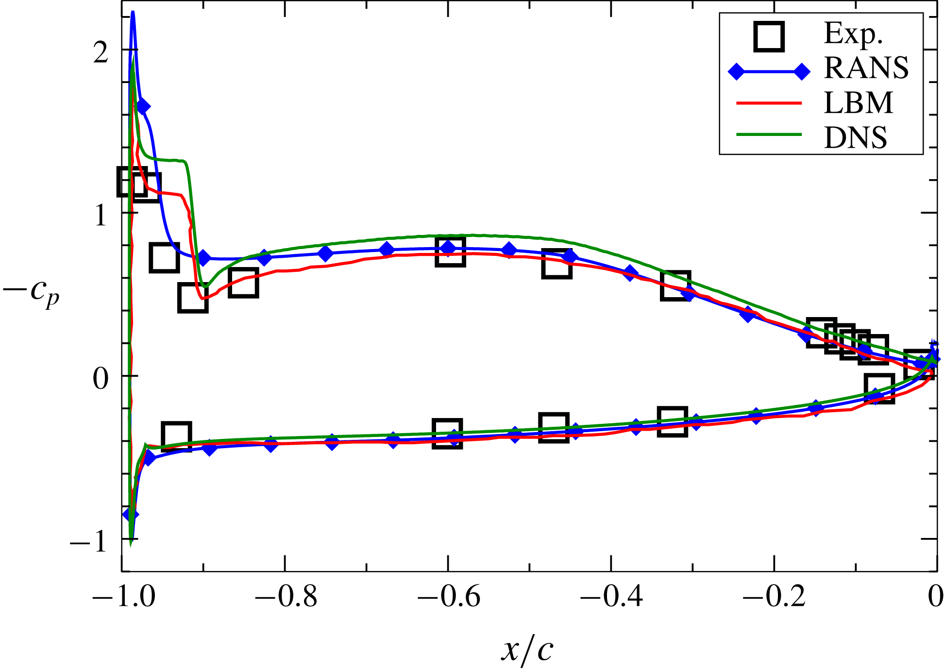
Secondly, to check whether the installation effects have been properly captured, the pressure distribution over the aerofoil is checked through the mean wall-pressure coefficient
 $c_{p}$
, which is defined as
 $$\begin{eqnarray}c_{p}=\frac{\overline{p}-p_{ref}}{\frac{1}{2}\unicode[STIX]{x1D70C}_{ref}u_{ref}^{2}},\end{eqnarray}$$
where
 $p_{ref}$
,
 $\unicode[STIX]{x1D70C}_{ref}$
and
 $u_{ref}$
are reference static pressure, air density and velocity. The DNS result is compared with wind-tunnel measurements, RANS calculations and a previous DNS using a lattice-Boltzmann method (LBM) (Sanjosé et al.
Reference Sanjosé, Moreau, Kim and Pérot2011) including the complete wind-tunnel nozzle and aerofoil geometry. The experimental data were recently produced at the Université de Sherbrooke (Padois et al.
Reference Padois, Laffay, Idier and Moreau2015) in a newly designed anechoic wind tunnel where a low background turbulence intensity
 $T_{u}$
can be achieved (
 $T_{u}=0.3{-}0.4\,\%$
).
Static lift distribution on the CD aerofoil from experiment, RANS (
 $k{-}\unicode[STIX]{x1D714}$
SST), LBM (Sanjosé et al.
Reference Sanjosé, Moreau, Kim and Pérot2011) and the current DNS (Wu et al.
Reference Wu, Sanjosé, Moreau and Sandberg2018).

As shown in figure 5, the current DNS produces a good prediction of
 $c_{p}$
. A slightly longer separation bubble is present in the current DNS, which does not account for the jet shear layers and the possible introduction of the free-stream turbulence that are present in experiments (Istvan, Kurelek & Yarusevych Reference Istvan, Kurelek and Yarusevych2017). In all, the current DNS is deemed reliable for further investigation on pressure-gradient effects for such a flow case.
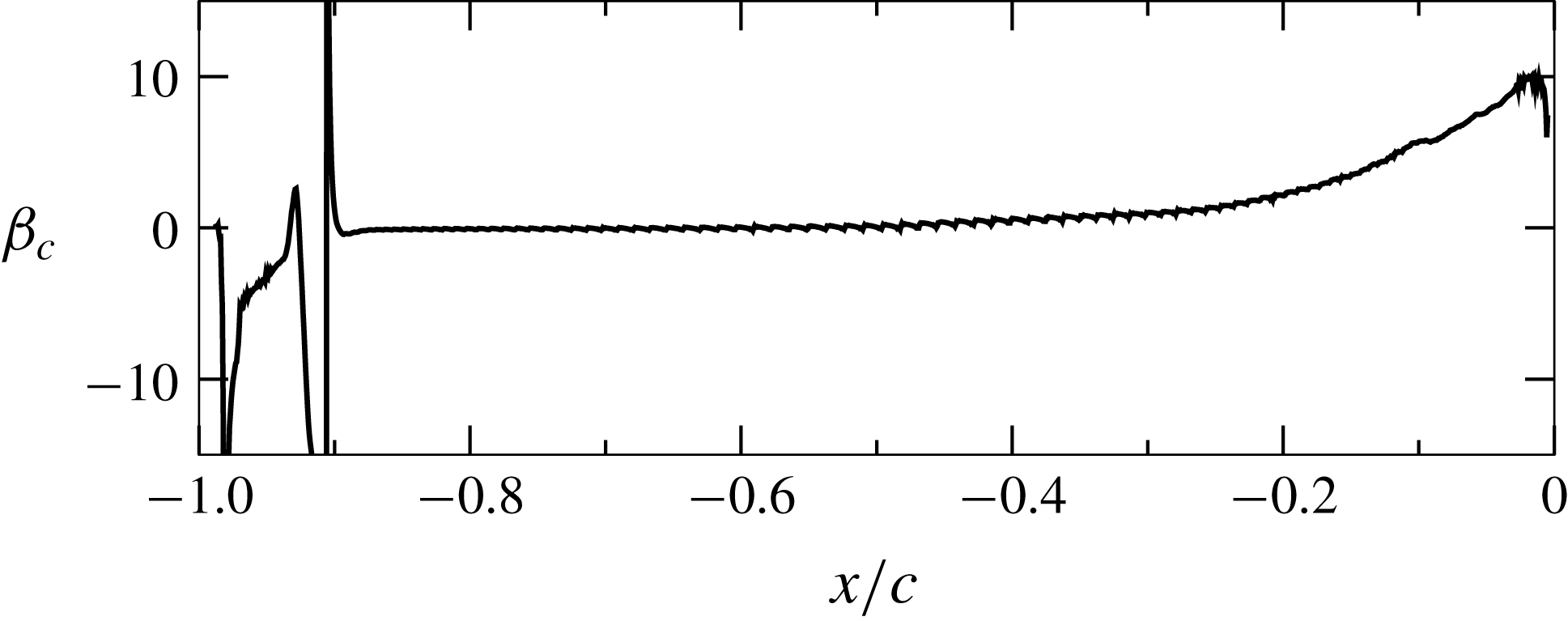
The dimensionless Clauser pressure-gradient parameter
 $\unicode[STIX]{x1D6FD}_{c}$
(Clauser Reference Clauser1956) is taken to quantify the distribution of the mean pressure gradients over the aerofoil suction side,
 $$\begin{eqnarray}\unicode[STIX]{x1D6FD}_{c}=\frac{\unicode[STIX]{x1D6FF}^{\ast }}{\unicode[STIX]{x1D70F}_{w}}\frac{\text{d}P}{\text{d}s_{w}},\end{eqnarray}$$
where
 $\unicode[STIX]{x1D6FF}^{\ast }$
is the displacement thickness,
 $\unicode[STIX]{x1D70F}_{w}$
is the wall shear stress and
 $\text{d}P/\text{d}s_{w}$
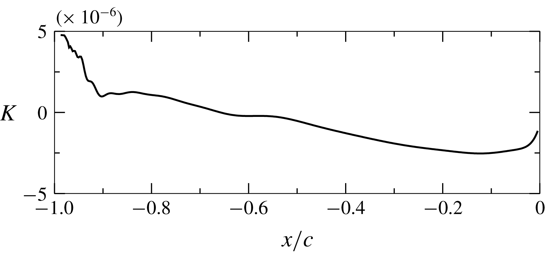
is the pressure gradient between two points on the surface of the aerofoil suction side. The acceleration level is evaluated by the acceleration parameter
 $K$
, defined as
 $$\begin{eqnarray}K=\frac{\unicode[STIX]{x1D708}}{U_{\infty }^{2}}\frac{\text{d}U_{\infty }}{\text{d}s_{w}},\end{eqnarray}$$
where
 $U_{\infty }^{2}$
is the local free-stream velocity magnitude where the edge velocity is obtained from wall-normal profiles,
 $\unicode[STIX]{x1D708}$
is the kinematic viscosity and
 $\text{d}s_{w}$
is the distance between two points on the surface of the aerofoil suction side. It should be mentioned that, in the original commonly used forms of
 $\unicode[STIX]{x1D6FD}_{c}$
and
 $K$
, the gradient terms are taken as the streamwise gradients
 $\text{d}P/\text{d}x$
and
 $\text{d}U_{\infty }/\text{d}x$
. They are adapted to the aerofoil case here with curvilinear forms
 $\text{d}U_{\infty }/\text{d}s_{w}$
and
 $\text{d}P/\text{d}s_{w}$
. As can be seen in figures 6 and 7, after the separation bubble at the LE, the flow develops firstly in a mild FPG zone where
 $\unicode[STIX]{x1D6FD}_{c}\approx -0.2$
and
 $K\approx 1.7\times 10^{-6}$
, followed by a ZPG zone at mid-chord, and finally in a strong APG zone where
 $\unicode[STIX]{x1D6FD}_{c}$
grows up to 10.0 and
 $K$
drops to
 $-2.5\times 10^{-6}$
. The
 $\unicode[STIX]{x1D6FD}_{c}$
values near the TE are very similar to previously reported results from LES (Christophe et al.
Reference Christophe, Moreau, Hamman, Witteveen and Iaccarino2014) on the same aerofoil.
Clauser pressure-gradient parameter
 $\unicode[STIX]{x1D6FD}_{c}$
(Clauser Reference Clauser1956) along the aerofoil suction side.

Acceleration parameter
 $K$
along the aerofoil suction side.

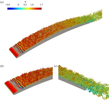
The flow topology is then shown by isocontours of the swirling strength criterion
 $\unicode[STIX]{x1D706}_{ci}$
(Zhou et al.
Reference Zhou, Adrian, Balachandar and Kendall1999; Wu et al.
Reference Wu, Moin, Wallace, Skarda, Lozano-Durán and Hickey2017) and coloured by the streamwise velocity component. As first proposed by Zhou et al. (Reference Zhou, Adrian, Balachandar and Kendall1999),
 $\unicode[STIX]{x1D706}_{ci}$
is the imaginary part of the complex eigenvalue of the velocity-gradient tensor
 $\unicode[STIX]{x1D63C}:=\unicode[STIX]{x1D735}\boldsymbol{u}$
when
 $\unicode[STIX]{x1D63C}$
is decomposed in Cartesian coordinates as
 $$\begin{eqnarray}\unicode[STIX]{x1D63C}=\left[\begin{array}{@{}ccc@{}}\boldsymbol{v}_{r} & \boldsymbol{v}_{cr} & \boldsymbol{v}_{ci}\end{array}\right]\left[\begin{array}{@{}ccc@{}}\unicode[STIX]{x1D706}_{r} & 0 & 0\\ 0 & \unicode[STIX]{x1D706}_{cr} & \unicode[STIX]{x1D706}_{ci}\\ 0 & -\unicode[STIX]{x1D706}_{ci} & \unicode[STIX]{x1D706}_{cr}\end{array}\right]\left[\begin{array}{@{}ccc@{}}\boldsymbol{v}_{r} & \boldsymbol{v}_{cr} & \boldsymbol{v}_{ci}\end{array}\right]^{\text{T}},\end{eqnarray}$$
where
 $\unicode[STIX]{x1D706}_{r}$
is the real eigenvalue corresponding to the eigenvector
 $\boldsymbol{v}_{r}$
, and
 $\unicode[STIX]{x1D706}_{cr}\pm \unicode[STIX]{x1D706}_{ci}\text{i}$
are the conjugate pair of the complex eigenvalues with eigenvectors
 $\boldsymbol{v}_{cr}\pm \boldsymbol{v}_{ci}\text{i}$
. In such a decomposition, as explained by Zhou et al. (Reference Zhou, Adrian, Balachandar and Kendall1999), the local streamlines can be expressed in the coordinate system defined by (
 $\boldsymbol{v}_{r},\boldsymbol{v}_{cr},\boldsymbol{v}_{ci}$
) such that the local flow is either stretched or compressed along the
 $\boldsymbol{v}_{r}$
axis, while on the plane spanned by the vectors
 $\boldsymbol{v}_{cr}$
and
 $\boldsymbol{v}_{ci}$
, the flow is swirling. The strength of the local swirling motion is then quantified by
 $\unicode[STIX]{x1D706}_{ci}$
.
The value of
 $\unicode[STIX]{x1D706}_{ci}$
is chosen such that it is approximately 3 % of its maximum value for the flow data around the aerofoil, similar to what has previously been suggested (Zhou et al.
Reference Zhou, Adrian, Balachandar and Kendall1999). On the suction side, it can be seen that at the LE, spanwise coherent roller structures are generated due to a Kelvin–Helmholtz instability and secondary instabilities which finally lead to a short recirculation bubble that triggers the transition. The initially large structures become smaller around mid-chord and then the flow further develops until the TE. Near the TE, the turbulent flow featuring hairpin structures from the suction side is mixed with the laminar flow from the pressure side in the near wake. The local Reynolds numbers based on the momentum thickness
 $\unicode[STIX]{x1D703}$
after the transition are
 $Re_{\unicode[STIX]{x1D703}}\sim 210{-}1206$
with a shape factor,
 $H=\unicode[STIX]{x1D6FF}^{\ast }/\unicode[STIX]{x1D703}$
, range
 $1.51{-}2.14$
, where
 $\unicode[STIX]{x1D6FF}^{\ast }$
is the displacement thickness. On the pressure side, the laminar boundary layer stays attached, and rolls up at the TE, leading to a weak vortex shedding in the near wake. These basic flow features are qualitatively very similar to the DNS using LBM mentioned before by Sanjosé et al. (Reference Sanjosé, Moreau, Kim and Pérot2011).
Swirling strength criterion
 $\unicode[STIX]{x1D706}_{ci}=70$
isocontours coloured by streamwise velocity: (a) aerofoil global view; (b) zoom view at LE; (c) zoom view at TE and near wake.

3 Compressible velocity-gradient tensor invariant dynamics
The velocity-gradient tensor
 $\unicode[STIX]{x1D63C}:=\unicode[STIX]{x1D735}\boldsymbol{u}$
is a
 $3\times 3$
matrix. According to its characteristic polynomial
 $p_{char}$
,
 $$\begin{eqnarray}p_{char}(\unicode[STIX]{x1D6FC}):=\text{det}(\unicode[STIX]{x1D63C}-\unicode[STIX]{x1D6FC}\unicode[STIX]{x1D644})=\unicode[STIX]{x1D6FC}^{3}+P\unicode[STIX]{x1D6FC}^{2}+Q\unicode[STIX]{x1D6FC}+R,\end{eqnarray}$$
where
 $\unicode[STIX]{x1D644}$
is the identity matrix and the first three invariants
 $P$
,
 $Q$
and
 $R$
can be calculated as
 $$\begin{eqnarray}\displaystyle & \displaystyle P=-\text{trace}(\unicode[STIX]{x1D63C})=-\unicode[STIX]{x1D735}\boldsymbol{\cdot }\boldsymbol{u}, & \displaystyle\end{eqnarray}$$
 $$\begin{eqnarray}\displaystyle & \displaystyle Q={\textstyle \frac{1}{2}}(\text{trace}(\unicode[STIX]{x1D63C})^{2}-\text{trace}(\unicode[STIX]{x1D63C}\unicode[STIX]{x1D63C}))={\textstyle \frac{1}{2}}(P^{2}-\text{trace}(\unicode[STIX]{x1D63C}^{2})), & \displaystyle\end{eqnarray}$$
 $$\begin{eqnarray}\displaystyle & \displaystyle R=-\text{det}(\unicode[STIX]{x1D63C})=-{\textstyle \frac{1}{3}}(P^{3}-3PQ+\text{trace}(\unicode[STIX]{x1D63C}^{3})). & \displaystyle\end{eqnarray}$$
 $p_{char}$
,
 $$\begin{eqnarray}\unicode[STIX]{x1D6E5}:=-{\textstyle \frac{1}{4}}P^{2}Q^{2}+Q^{3}+P^{3}R+{\textstyle \frac{27}{4}}R^{2}-{\textstyle \frac{18}{4}}PQR.\end{eqnarray}$$
 $\unicode[STIX]{x1D63C}$
has its own dynamics defined as
 $$\begin{eqnarray}\frac{\text{d}\unicode[STIX]{x1D63C}}{\text{d}t}:=\frac{\unicode[STIX]{x2202}\unicode[STIX]{x1D63C}}{\unicode[STIX]{x2202}t}+(\boldsymbol{u}\boldsymbol{\cdot }\unicode[STIX]{x1D735})\unicode[STIX]{x1D63C}=-\unicode[STIX]{x1D63C}\unicode[STIX]{x1D63C}+\unicode[STIX]{x1D643}.\end{eqnarray}$$
Here the source term
 $\unicode[STIX]{x1D643}$
 $$\begin{eqnarray}\unicode[STIX]{x1D643}:=\unicode[STIX]{x1D71E}-\unicode[STIX]{x1D72E}\end{eqnarray}$$
is a combination of the viscous effects
 $\unicode[STIX]{x1D71E}$
and the pressure–density term
 $\unicode[STIX]{x1D72E}$
defined as
 $$\begin{eqnarray}\displaystyle & \displaystyle \unicode[STIX]{x1D71E}=\unicode[STIX]{x1D735}\left(\frac{1}{\unicode[STIX]{x1D70C}}\unicode[STIX]{x1D735}\boldsymbol{\cdot }\unicode[STIX]{x1D749}\right), & \displaystyle\end{eqnarray}$$
 $$\begin{eqnarray}\displaystyle & \displaystyle \unicode[STIX]{x1D72E}=\unicode[STIX]{x1D735}\left(\frac{1}{\unicode[STIX]{x1D70C}}\unicode[STIX]{x1D735}p\right). & \displaystyle\end{eqnarray}$$
With these notions set, the compressible velocity-gradient tensor invariant dynamics system can be described as
 $$\begin{eqnarray}\displaystyle & \displaystyle \frac{\text{d}P}{\text{d}t}=P^{2}-2Q-\text{trace}(\unicode[STIX]{x1D643}), & \displaystyle\end{eqnarray}$$
 $$\begin{eqnarray}\displaystyle & \displaystyle \frac{\text{d}Q}{\text{d}t}=QP-\frac{2}{3}P\,\text{trace}(\unicode[STIX]{x1D643})-3R-\text{trace}(\unicode[STIX]{x1D63C}\unicode[STIX]{x1D643}^{\ast }), & \displaystyle\end{eqnarray}$$
 $$\begin{eqnarray}\displaystyle & \displaystyle \frac{\text{d}R}{\text{d}t}=-\frac{1}{3}Q\,\text{trace}(\unicode[STIX]{x1D643})+PR-P\,\text{trace}(\unicode[STIX]{x1D63C}\unicode[STIX]{x1D643}^{\ast })-\text{trace}(\unicode[STIX]{x1D63C}^{2}\unicode[STIX]{x1D643}^{\ast }), & \displaystyle\end{eqnarray}$$
 $\unicode[STIX]{x1D643}^{\ast }$
is the traceless part from the decomposition of the pressure and viscous stress matrix
 $\unicode[STIX]{x1D643}$
,
 $$\begin{eqnarray}\unicode[STIX]{x1D643}=\unicode[STIX]{x1D643}^{\ast }+{\textstyle \frac{1}{3}}\,\text{trace}(\unicode[STIX]{x1D643})\unicode[STIX]{x1D644}.\end{eqnarray}$$
In this work, all separate terms are available from the DNS dataset described in § 2 and consequently this system can be fully exploited for the interpretation of the flow over the aerofoil. As shown above in this section, all the terms in the velocity-gradient invariants dynamics system are derived with no assumption on incompressibility. However, for weakly compressible cases, such as the present flow field around the CD aerofoil, the first invariant
 $P$
, as well as its derivatives, can be assumed to have much smaller magnitude than the second and third invariants. This assumption will be checked and explained in § 4.3. Consequently, the
 $PQR$
space can be mapped into one of its subsets defined by
 $P=0$
and the analysis will not be extended to the first invariant dynamics.
4 Results
We first focus on the mean profiles from the investigated areas of flow over the CD aerofoil, followed by the overall Lagrangian dynamics at different locations along the aerofoil. Then the contributions of the separate terms of the overall dynamics are discussed and the influence of different pressure-gradient conditions are addressed. Finally, the wall effects are discussed by comparison of the flow at the aerofoil TE and that in the near wake.
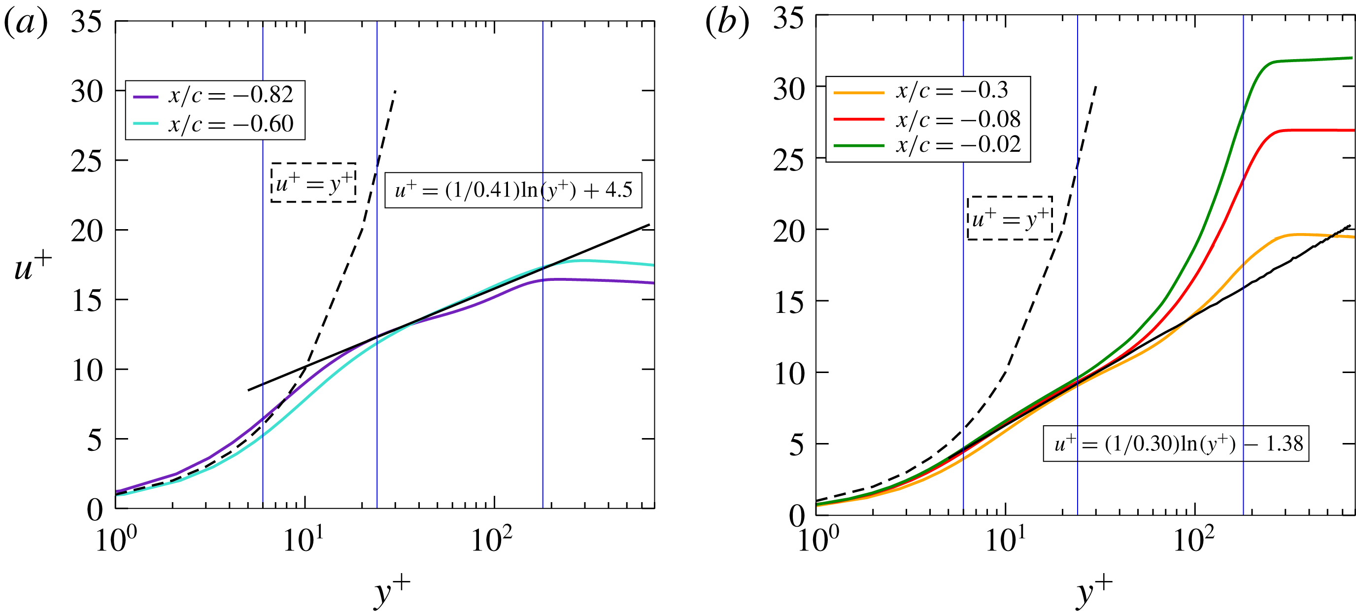
Profiles of the mean wall tangential velocity along wall-normal distance: (a) FPG (
 $x/c=-0.82$
,
 $18\,\%$
chord) and ZPG zones (
 $x/c=-0.60$
,
 $40\,\%$
chord) at
 $Re_{\unicode[STIX]{x1D703}}=210$
and 280, respectively; (b) APG zones (
 $x/c=-0.3$
,
 $70\,\%$
chord;
 $x/c=-0.08$
,
 $92\,\%$
chord;
 $x/c=-0.02$
,
 $98\,\%$
chord) at
 $Re_{\unicode[STIX]{x1D703}}=621$
, 1009 and 1187, respectively.

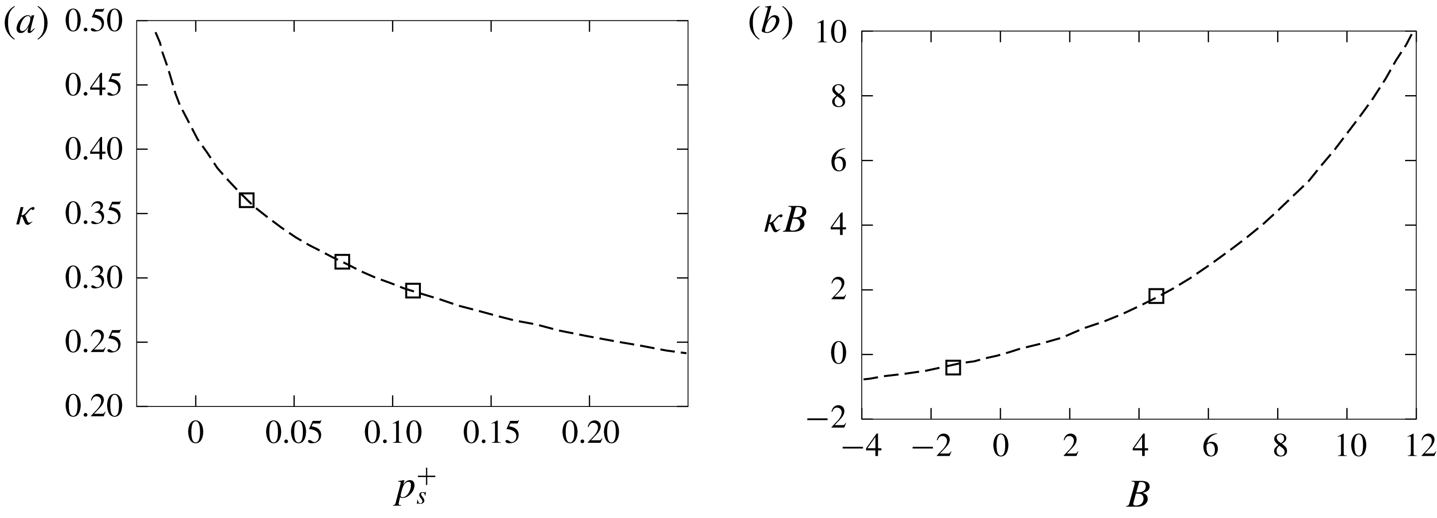
Curve fits from literature. (a) Curve fit obtained from figure 8 and equation (7.5) in Nickels (Reference Nickels2004) (– – – –) and from current DNS (▫). Values of
 $\unicode[STIX]{x1D705}$
and
 $p_{s}^{+}$
from APG zones (
 $x/c=-0.3$
,
 $70\,\%$
chord;
 $x/c=-0.08$
,
 $92\,\%$
chord;
 $x/c=-0.02$
,
 $98\,\%$
chord) in figure 9. (b) Curve fit from figure 5 in Nagib & Chauhan (Reference Nagib and Chauhan2008) (– – – –) and from current DNS (▫). Values of
 $\unicode[STIX]{x1D705}$
and
 $B$
of the current DNS are from solid black lines in figure 9: (
 $\unicode[STIX]{x1D705}=0.41,~B=4.5$
) and (
 $\unicode[STIX]{x1D705}=0.30,~B=-1.38$
).

4.1 Mean flow profiles
In figure 9, the mean wall-normal velocity profiles are presented. The vertical blue lines mark the wall-normal locations that are chosen for further analysis in the following sections. These locations are, respectively, in the viscous sublayer, log layer and outer layer spanning a range of
 $y^{+}$
from 6 to 180. It can be seen that the pressure gradient dramatically changes the log layer and outer layer for these five investigated locations. The typical von Kármán constant
 $\unicode[STIX]{x1D705}=0.41$
for the classical law of the wall (Von Kármán Reference von Kármán1931),
 $$\begin{eqnarray}u^{+}=\frac{1}{\unicode[STIX]{x1D705}}\ln (y^{+})+B,\end{eqnarray}$$
works well in the ZPG zones. Yet, for FPG and APG zones, variations of this value have been reported. Nagib & Chauhan (Reference Nagib and Chauhan2008) have emphasized the non-universality of the von Kármán constant
 $\unicode[STIX]{x1D705}$
through various experiments on canonical flows and showed that FPG leads to higher values of
 $\unicode[STIX]{x1D705}$
while APG gives lower
 $\unicode[STIX]{x1D705}$
. They also showed that the constant
 $B$
can be negative, which is the case for the current flow. This is also consistent with the variations reported by Nickels (Reference Nickels2004) (figure 8 therein), which is repeated here for the present dimensionless pressure gradients
 $p_{s}^{+}=(\unicode[STIX]{x1D708}/\unicode[STIX]{x1D70C}u_{\unicode[STIX]{x1D70F}}^{3})(\text{d}p/\text{d}s)$
in figure 10(a). Yet, the values for von Kármán constant
 $\unicode[STIX]{x1D705}$
obtained from this aerofoil case in APG zones are quite different from some earlier reported works of APG boundary layers from flat plates (Lee & Sung Reference Lee and Sung2008; Knopp et al.
Reference Knopp, Schanz, Schröder, Dumitra, Cierpka, Hain and Kähler2014). They, however, correspond to quite different flow conditions. Either
 $\unicode[STIX]{x1D6FD}_{c}$
is much smaller (Lee & Sung Reference Lee and Sung2008) or the local Reynolds number
 $Re_{\unicode[STIX]{x1D703}}$
is much higher (Knopp et al.
Reference Knopp, Schanz, Schröder, Dumitra, Cierpka, Hain and Kähler2014). Yet they all lie on the curve fit proposed by Nagib & Chauhan (Reference Nagib and Chauhan2008) for many FPG, ZPG and APG boundary layers as shown in figure 10(b). Moreover, as mentioned by Lissaman (Reference Lissaman1983) in a review of low-Reynolds-number aerofoils, due to the aerofoil thickness and the angle of attack, for the flow over aerofoils, the turbulent boundary layer after transition can negotiate quite severe APG without separation. This is in essence quite different from flow cases from flat plates for similar pressure gradients. This phenomenon is actually shown in figure 6 as the DNS APG near the TE exhibits a high level while the flow is still attached to the aerofoil surface. Actually, it is one of the design objectives of CD aerofoils to provide higher loading capacity at low Mach numbers (Hobbs & Weingold Reference Hobbs and Weingold1984), which then gives higher pressure gradients. Vinuesa et al. (Reference Vinuesa, Örlü, Vila, Ianiro, Discetti and Schlatter2017) compared a set of high-quality DNS results for similar local
 $Re_{\unicode[STIX]{x1D703}}$
range APG boundary layers. They, for instance, pinpointed that the data from a DNS (Hosseini et al.
Reference Hosseini, Vinuesa, Schlatter, Hanifi and Henningson2016) over a NACA4412 aerofoil at
 $5^{\circ }$
angle of attack show much severer APG measured by
 $\unicode[STIX]{x1D6FD}_{c}$
for similar
 $Re_{\unicode[STIX]{x1D703}}$
range. The strong APG over the aerofoil exhibited a significant effect in the outer flow, and was also noticeable in the incipient logarithmic region and all the way down to the buffer layer. Taking that the CD aerofoil from the current DNS has a blade shape, which has an even higher camber and is operated at a higher angle of attack than the case reported by Hosseini et al. (Reference Hosseini, Vinuesa, Schlatter, Hanifi and Henningson2016), the deviation of the mean velocity profiles from the standard form is therefore expected.
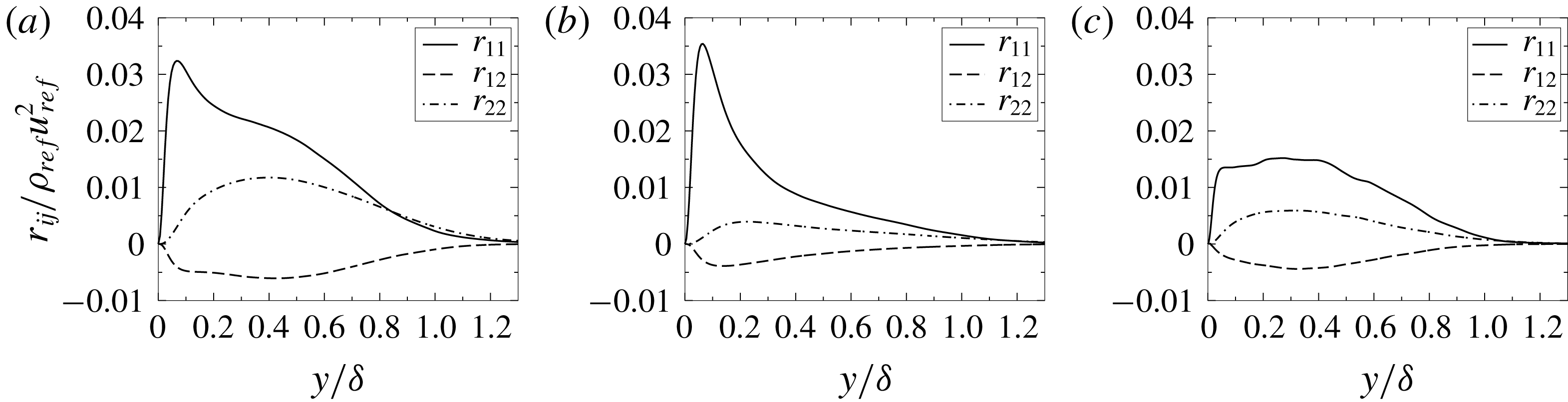
Reynolds stress components normalized with outer scale along wall-normal direction: (a) FPG, (b) ZPG zones and (c) APG zones.

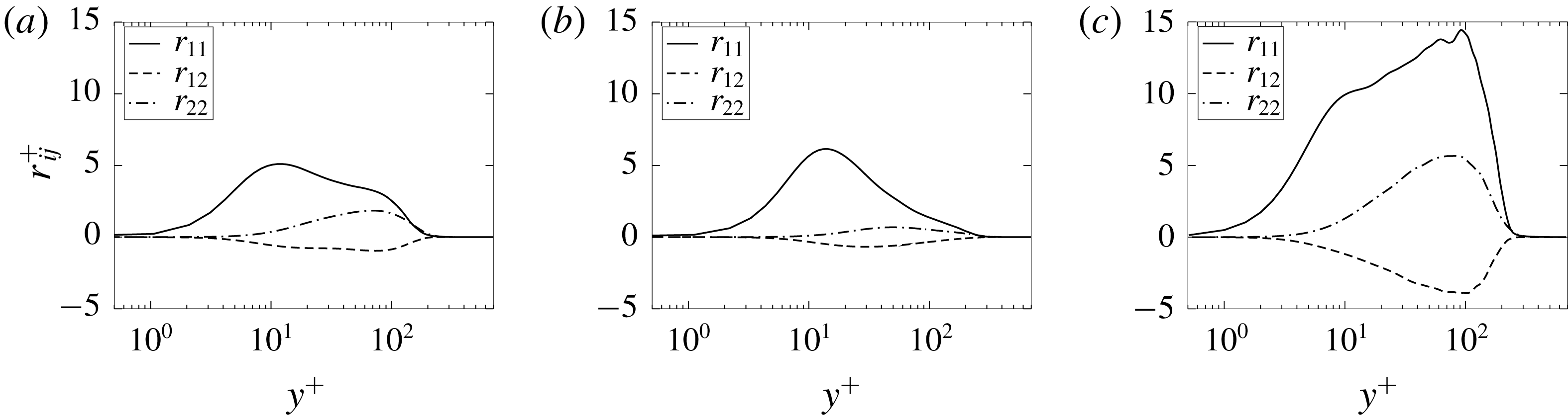
Reynolds stress components normalized with inner scale along wall-normal direction: (a) FPG, (b) ZPG zones and (c) APG zones.

The Reynolds stress components
 $r_{ij}$
are shown in figures 11 and 12. Here the indices
 $1$
and
 $2$
, which appear in the legends for
 $r_{ij}$
, refer to the wall-parallel and wall-normal directions, respectively. In these two figures the wall-normal distance is scaled with the boundary layer thickness
 $\unicode[STIX]{x1D6FF}$
and the friction velocity
 $u_{\unicode[STIX]{x1D70F}}$
, respectively, to demonstrate the relative locations of the peaks; and
 $r_{ij}^{+}$
refers to the Reynolds stress components normalized by
 $\unicode[STIX]{x1D70C}u_{\unicode[STIX]{x1D70F}}^{2}$
. The boundary layer thickness
 $\unicode[STIX]{x1D6FF}=\unicode[STIX]{x1D6FF}_{p99}$
is determined by total pressure
 $p_{t}=(\unicode[STIX]{x1D70C}u^{2}+p_{s})/2$
, where
 $p_{s}$
is the static pressure at a certain point. The boundary layer reaches its limit when
 $p_{t}$
reaches
 $99\,\%$
of its maximum constant value along the wall-normal direction. It is necessary to use
 $\unicode[STIX]{x1D6FF}_{p99}$
not
 $\unicode[STIX]{x1D6FF}_{99}$
, the boundary layer thickness determined by
 $99\,\%$
of the tangential velocity maximum along a certain wall-normal direction, as a reference to calculate the boundary layer thickness because, for loaded aerofoils, the external flow is deflected and will therefore have a non-constant value. Thus, the velocity reference would give a boundary layer thickness much thicker than that obtained by using the total pressure. As shown in figures 11 and 12, the locations of the peak values of
 $r_{ij}$
, which present the most intense momentum transfer by fluctuating velocities in a turbulent boundary layer, also exhibit a significant change due to the presence of pressure gradients. For the ZPG, the peak values are usually in the viscous sublayer. This is the case for the data shown here in figures 11(b) and 12(b) for the flow at the LE and around mid-chord. Further downstream, with the increase of APG, the flow decelerates and the peak values of
 $r_{ij}$
extend to the log layer and even into the edge of the outer layer shown as a platform shape in figures 11(c) and 12(c) for
 $8\leqslant y^{+}\leqslant 103$
, which indicates that the APG acts as an additional factor to help the momentum exchange by fluctuating velocities. This platform shape is consistent with what has been reported by Lee & Sung (Reference Lee and Sung2008) at a similar
 $Re_{\unicode[STIX]{x1D703}}$
range and by Skaare & Krogstad (Reference Skaare and Krogstad1994) at a much higher
 $Re_{\unicode[STIX]{x1D703}}$
for an APG flow near separation. As mentioned by Lee & Sung (Reference Lee and Sung2009) from an APG with similar
 $Re_{\unicode[STIX]{x1D703}}$
from an incompressible DNS approach, hairpin-type vortices are the predominant structures associated with the production of Reynolds stress in the APG flows. The hairpin structures away from the wall in the TE region seen in figure 8(c) support such an argument for the origin of the outer peak of the Reynolds stress in APG. These Reynolds stress profiles further confirm the information presented in figure 4: the intense turbulent mixing for APG zones exists in both the viscous sublayer and the log layer, and even extend to the outer layer.
4.2 Pressure-gradient effects on mean
 $QR$
evolution as a function of wall-normal distance

For the following analysis, the flow data length scale is firstly rescaled from the initial chord length to the local boundary layer thickness
 $\unicode[STIX]{x1D6FF}=\unicode[STIX]{x1D6FF}_{p99}$
. Secondly, we introduce a scaling based on the local variance of the velocity-gradient tensor magnitude
 $$\begin{eqnarray}\text{var}(\unicode[STIX]{x1D63C})=\overline{\text{trace}((\unicode[STIX]{x1D63C}-\overline{\unicode[STIX]{x1D63C}})(\unicode[STIX]{x1D63C}-\overline{\unicode[STIX]{x1D63C}})^{\text{T}})}.\end{eqnarray}$$
This is a measure of the variation of the velocity-gradient tensor magnitude and it can be regarded as a gradient analogue to the TKE. Consequently, the related terms in the
 $QR$
space are scaled as
 $\hat{\unicode[STIX]{x1D63C}}=\unicode[STIX]{x1D63C}/\sqrt{\text{var}(\unicode[STIX]{x1D63C})}$
,
 $\hat{\boldsymbol{Q}}=\boldsymbol{Q}/\text{var}(\unicode[STIX]{x1D63C})$
and
 $\hat{\boldsymbol{R}}=\boldsymbol{R}/\text{var}(\unicode[STIX]{x1D63C})^{3/2}$
. The p.d.f. values for the
 $QR$
plots in this paper are multiplied by 10 and normalized by the local maximum p.d.f. value and the colour bars are plotted using a logarithmic scale from 0 to 1.
Lozano-Durán, Holzner & Jiménez (Reference Lozano-Durán, Holzner and Jiménez2015) state that integrating over a statistically inhomogeneous region can considerably bias the Lagrangian statistics. To avoid this bias, the investigated regions in this work are chosen so that the turbulence within the integration area is regarded as quasi-statistically homogeneous. This is achieved by following the procedure reported in Bechlars & Sandberg (Reference Bechlars and Sandberg2017a
). The mean dynamics data presented in this work were integrated in the homogeneous spanwise direction, about an extent of approximately 20 grid points in the streamwise direction and approximately five grid points in the wall-normal direction for each location. This results in
 $\unicode[STIX]{x0394}x^{+}\approx 100$
and
 $\unicode[STIX]{x0394}y^{+}\approx 6$
for the location at
 $y^{+}=24$
. These distances are similar to those in the work of Bechlars & Sandberg (Reference Bechlars and Sandberg2017a
).
As mentioned in previous studies, the teardrop shape is not a universal feature, which is often observed for homogeneous isotropic turbulent (HIT) flows. For wall-bounded flows, the mean evolution of the velocity-gradient tensor invariants has been found to vary strongly with the distance to the wall (Bechlars & Sandberg Reference Bechlars and Sandberg2017a ). This wall effect is observed for all investigated locations in this aerofoil case.
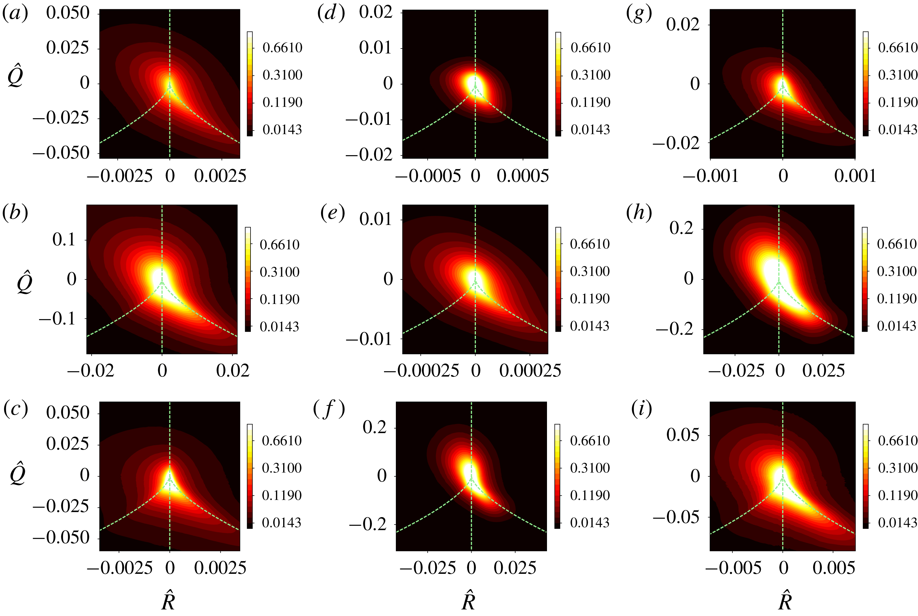
The mean
 $QR$
development with distance to the wall over the CD aerofoil. From left to right: FPG (
 $18\,\%$
chord), ZPG (
 $40\,\%$
chord) and APG (
 $92\,\%$
chord) zones. Three wall-normal locations are shown: (a,d,g)
 $y^{+}\approx 6$
, (b,e,h)
 $y^{+}\approx 24$
, and (c,f,i)
 $y^{+}\approx 180$
. The dashed lines divide the
 $QR$
space into four sectors which cover, respectively, a certain flow topology as mentioned in § 1.

Figure 13 shows the overall
 $QR$
distribution, in which each row corresponds to regions at
 $18\,\%$
,
 $40\,\%$
and
 $92\,\%$
of the aerofoil chord from FPG to APG zones (left to right) and each column corresponds to a certain region from
 $y^{+}\approx 6$
to
 $y^{+}\approx 180$
(top to bottom). The contours cover
 $95\,\%$
of the events, which means that the black colour represents only
 $5\,\%$
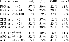
of the maximum p.d.f. value in each plot. Moreover, to obtain a more quantitative impression, the joint p.d.f. is integrated over the respective sectors in
 $QR$
space as mentioned in § 1 to calculate the ratio of occurrence from all events in each sector. This is shown in table 1. It can be seen that the Lagrangian dynamics in these three zones have rather different behaviours. In the FPG zone, an oval shape is seen for the location closest to the wall. In the log layer, the teardrop shape is observed. In the outer layer, the contracting vortical mechanism is less present, as can be seen from table 1, which then gives the
 $QR$
plot a quasi-triangular shape. The shapes seen in the ZPG regions resemble the shapes that were reported in Bechlars & Sandberg (Reference Bechlars and Sandberg2017a
): the outer layer matches the teardrop shape from HIT data in the literature and becomes oval on approaching the wall. The APG has the effect that the
 $QR$
shape of the outer layer becomes concentrated around the
 $\unicode[STIX]{x1D6E5}=0$
line with positive
 $R$
values which is the dividing line of sectors representing the vortical contracting manner and pure straining with flattening character. This means that the energy exchange between the mean kinetic energy and the TKE is stronger than in the case of the ZPG. It is well established that vortex stretching is a major mechanism of the cascading process towards smaller scales. Figure 13(i) suggests that this behaviour is suppressed by the APG as there are fewer events present in the
 $\unicode[STIX]{x1D6E5}>0$
,
 $R\leqslant 0$
sector especially for positive
 $Q$
values, as there are fewer bright areas in the
 $S$
I sector compared with figure 13(f). This is also quantitatively reflected in table 1 when comparing the percentage in
 $S$
I between APG and ZPG at
 $y^{+}\approx 180$
. Closer to the wall at
 $y^{+}\approx 24$
in the log layer, for positive
 $R$
values, more flattening strain and less contracting vortical structures are present compared to the ZPG zone with the same wall-normal location. The region closest to the wall produces a
 $QR$
plot with similar shape to that obtained from the ZPG region. This again indicates that the APG acts as a strong mixing reinforcement in the outer layer and log layer for this turbulent boundary layer. In all, it can be concluded that, from the
 $QR$
point of view, the viscous sublayer has an invariant character: oval shape independent of the pressure-gradient conditions. Yet the log layer and the outer layer strongly depend on the pressure gradient.
Ratios of the characteristic flow topologies in four sectors as mentioned in § 1 in the
 $QR$
space from sampling locations over the aerofoil: FPG,
 $18\,\%$
chord; ZPG,
 $40\,\%$
chord; and APG,
 $92\,\%$
chord.

4.3 Component analysis: nonlinearity, viscous and pressure effects
In this part, the contribution from separate terms of the compressible evolution system in (3.7) is studied. For this purpose, three groups of evolution terms are identified as suggested by Bechlars & Sandberg (Reference Bechlars and Sandberg2017a ):
(i)
$\unicode[STIX]{x1D643}^{\ast }=0$
;(ii)
$\text{trace}(\unicode[STIX]{x1D643})=\unicode[STIX]{x1D72E}=Q=R=0$
;(iii)
$\text{trace}(\unicode[STIX]{x1D643})=\unicode[STIX]{x1D71E}=Q=R=0$
.


These give the simplified invariant dynamics systems from (3.7):
(i)
(4.3a )$$\begin{eqnarray}\displaystyle & \displaystyle \frac{\text{d}Q}{\text{d}t}=QP-\frac{2}{3}P\,\text{trace}(\unicode[STIX]{x1D643})-3R, & \displaystyle\end{eqnarray}$$
(4.3b )$$\begin{eqnarray}\displaystyle & \displaystyle \frac{\text{d}R}{\text{d}t}=-\frac{1}{3}Q\,\text{trace}(\unicode[STIX]{x1D643})+PR; & \displaystyle\end{eqnarray}$$
(ii)
(4.4a )$$\begin{eqnarray}\displaystyle & \displaystyle \frac{\text{d}Q}{\text{d}t}=-\text{trace}(\unicode[STIX]{x1D63C}\unicode[STIX]{x1D71E}^{\ast }), & \displaystyle\end{eqnarray}$$
(4.4b )$$\begin{eqnarray}\displaystyle & \displaystyle \frac{\text{d}R}{\text{d}t}=-\text{trace}(\unicode[STIX]{x1D63C}\unicode[STIX]{x1D63C}\unicode[STIX]{x1D71E}^{\ast }); & \displaystyle\end{eqnarray}$$
(iii)
Here(4.5a )$$\begin{eqnarray}\displaystyle & \displaystyle \frac{\text{d}Q}{\text{d}t}=\text{trace}(\unicode[STIX]{x1D63C}\unicode[STIX]{x1D72E}^{\ast }), & \displaystyle\end{eqnarray}$$
(4.5b )$$\begin{eqnarray}\displaystyle & \displaystyle \frac{\text{d}R}{\text{d}t}=\text{trace}(\unicode[STIX]{x1D63C}\unicode[STIX]{x1D63C}\unicode[STIX]{x1D72E}^{\ast }). & \displaystyle\end{eqnarray}$$
$\unicode[STIX]{x1D71E}^{\ast }$
and
$\unicode[STIX]{x1D72E}^{\ast }$
are the traceless parts of
$\unicode[STIX]{x1D71E}$
and
$\unicode[STIX]{x1D72E}$
defined in (3.6).


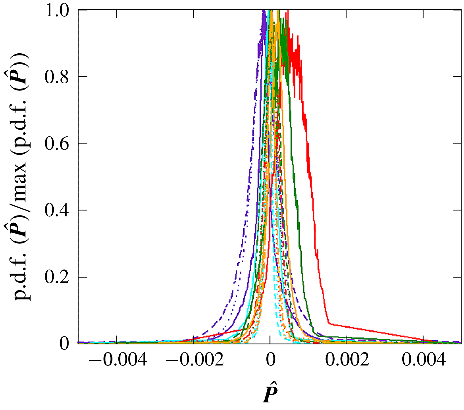
Ratios of the p.d.f. of the normalized first velocity-gradient invariant
 $\hat{\boldsymbol{P}}$
divided by the maximum values for the different zones over the aerofoil. Colours follow the legends in figure 9 (
 $\cdots \cdots$
,
 $y^{+}\approx 6$
; – – – –,
 $y^{+}\approx 24$
; ——,
 $y^{+}\approx 180$
).

Group (i) covers all the nonlinear terms, except the traceless part of the source term
 $\unicode[STIX]{x1D643}$
. For incompressible flows, this gives
 $\text{trace}(\unicode[STIX]{x1D643})=-2Q$
and the system would reduce to the restricted Euler system. For the current flow with low Mach number
 $M=0.25$
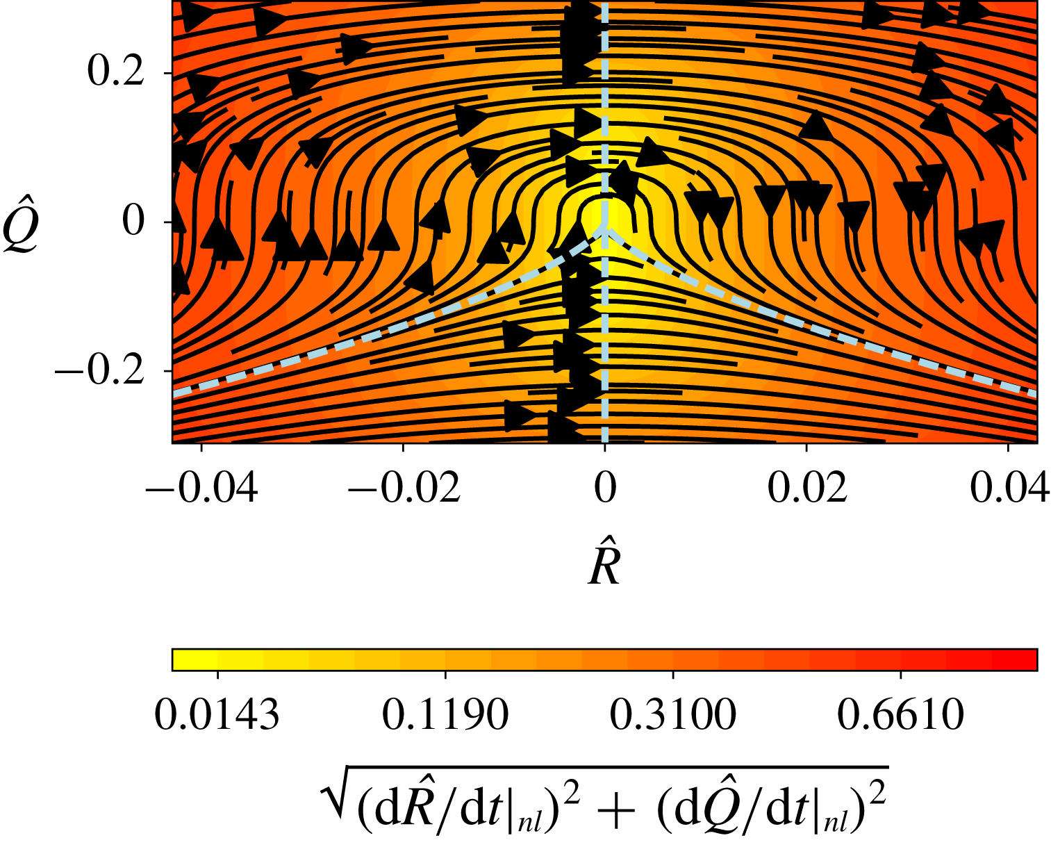
, the compressibility effects are small. For the evolution equations restricted to the nonlinear terms (as shown in figure 15) this means that there are no significant differences with the restricted Euler system (Vieillefosse Reference Vieillefosse1984). Data plotted in figure 15 are from
 $92\,\%$
chord in the APG zone at
 $y^{+}\approx 24$
. The trajectories (black streamlines) caused by nonlinear effects are very similar to those described by Vieillefosse (Reference Vieillefosse1984). Here only data from
 $92\,\%$
chord in the APG zone at
 $y^{+}\approx 24$
are shown but the contribution from nonlinear terms from all other investigated locations in the FPG, ZPG and APG zones shows an invariant character. This agreement with the incompressible reference (Vieillefosse Reference Vieillefosse1984) means that the mapping of the
 $PQR$
space to one of its subsets, the
 $QR$
space taking
 $P=0$
for such a low-Mach-number case, is valid. This has also been demonstrated by Bechlars & Sandberg (Reference Bechlars and Sandberg2017a
) for
 $M=0.5$
turbulent boundary layer data. Moreover, as shown in figure 14, the p.d.f. of the normalized first velocity-gradient invariant
 $\hat{\boldsymbol{P}}=\boldsymbol{P}/\sqrt{\text{var}(\unicode[STIX]{x1D63C})}$
, or normalized inverse dilatation, of all the investigated regions over the aerofoil exhibits very low absolute
 $\hat{\boldsymbol{P}}$
values (less than 0.002) for their maximum p.d.f. locations. This confirms that, as mentioned by Suman & Girimaji (Reference Suman and Girimaji2010) in terms of velocity-gradient invariant analysis, at low positive or negative dilatations, the statistical behaviour is similar to that in incompressible flow. In figure 15, the mean trajectories move from negative
 $R$
values towards positive, forming a round head when
 $Q$
values increase. The evolution velocity magnitude of the restricted Euler system is small around the origin of the
 $QR$
space and increases with the distance to the origin. Together with the global
 $QR$
plots shown in figure 13, it can also be seen that the nonlinear part drives the global shape of the
 $QR$
plots.
Nonlinearity effects: the mean
 $QR$
phase development is shown by trajectories (black) and by the magnitude of the mean phase velocity (contours) restricted to the nonlinear terms of the Navier–Stokes equations. The dashed lines divide the
 $QR$
space into four sectors which cover, respectively, a certain flow topology as mentioned in § 1.

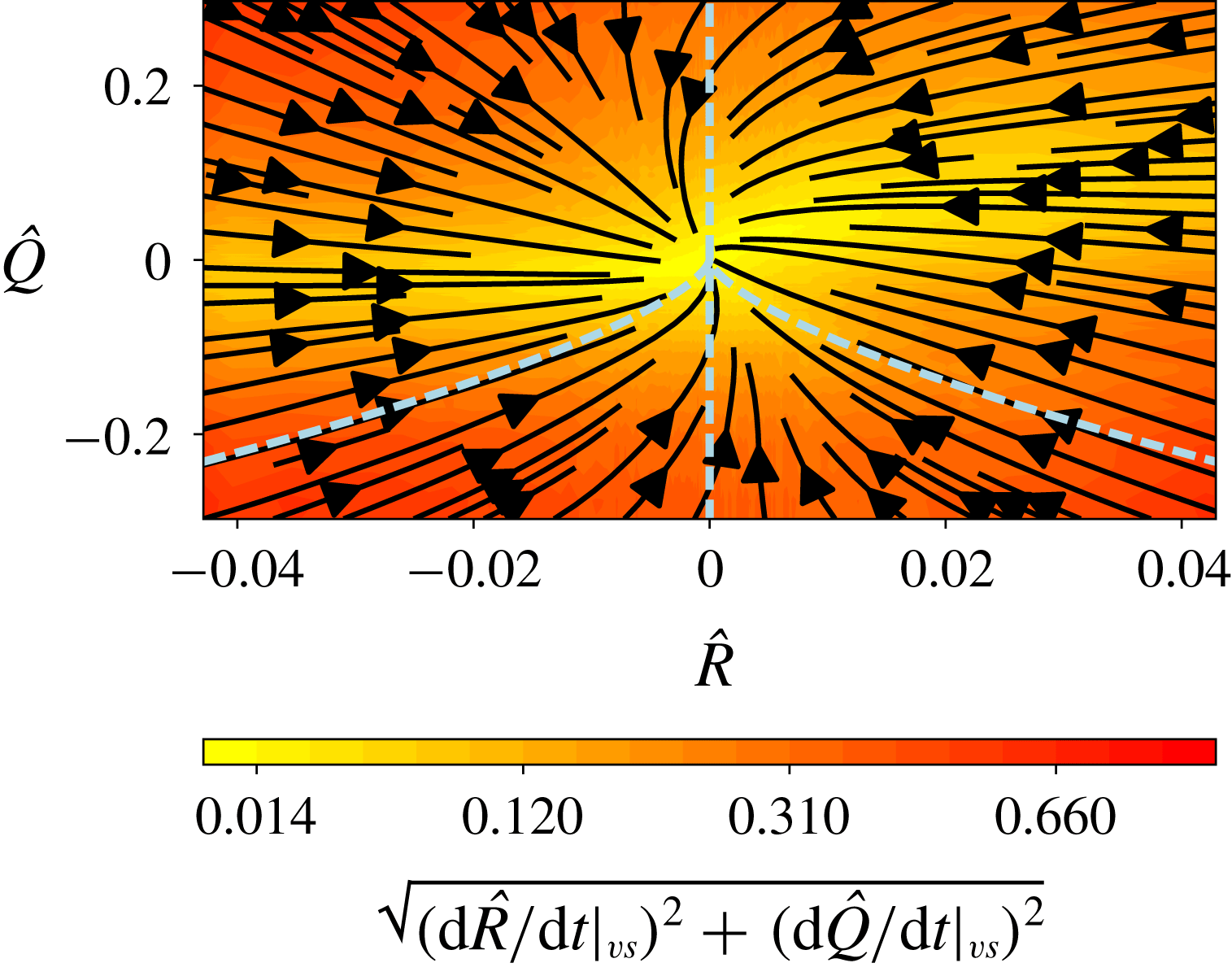
Viscous effects: the mean
 $QR$
phase development is shown by trajectories (black) and by the magnitude of the mean phase velocity (contours) restricted to the viscous terms of the Navier–Stokes equations. The dashed lines divide the
 $QR$
space into four sectors which cover, respectively, a certain flow topology as mentioned in § 1.

Group (ii) presents the viscous effects by neglecting all terms except the terms that link the viscous diffusion and the velocity-gradient tensor. This part also shows an invariant characteristic across the boundary layer for all investigated regions. Figure 16 is a representative
 $QR$
plot of this group. The data are extracted at
 $92\,\%$
chord in the APG zone at
 $y^{+}\approx 24$
. The trajectories are relatively straight, pointing towards the origin and only show a slight anticlockwise spin. The evolution velocity magnitude is decreasing with decreasing distance to the origin. But overall the restricted viscous diffusion evolution has an invariant character in this turbulent flow across the aerofoil regardless of the pressure-gradient conditions. The nonlinear terms and viscous terms are thus not the major reasons for the change of overall
 $QR$
distribution in these investigated zones.
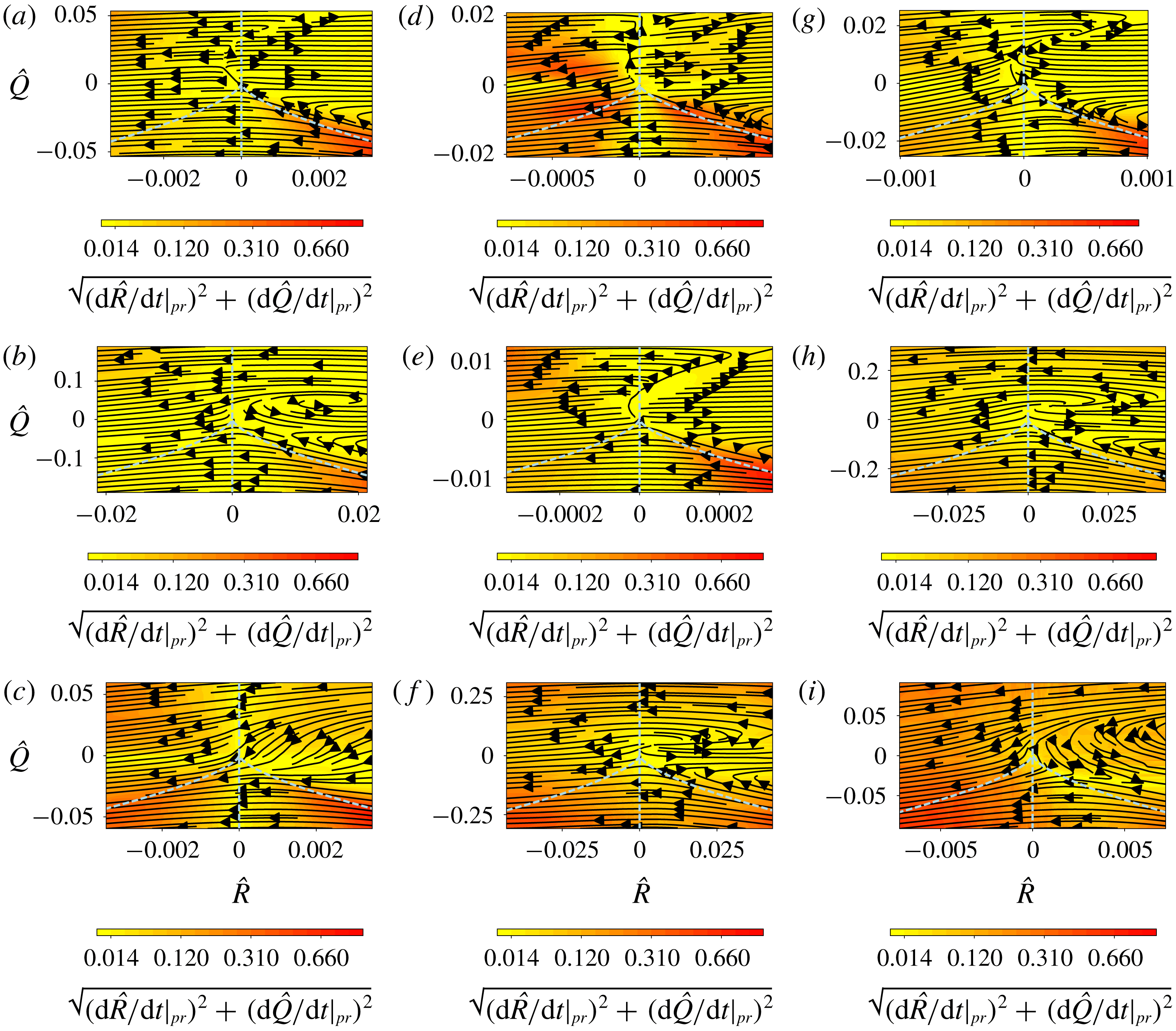
Pressure effects: the mean
 $QR$
phase development is shown by trajectories (black) and by the magnitude of the mean phase velocity (contours) restricted to the pressure term of the Navier–Stokes equations, respectively. From left to right: FPG (
 $18\,\%$
chord), ZPG (
 $40\,\%$
chord) and APG (
 $92\,\%$
chord) zones. Three wall-normal locations are shown: (a,d,g)
 $y^{+}\approx 6$
, (b,e,h)
 $y^{+}\approx 24$
, and (c,f,i)
 $y^{+}\approx 180$
. The dashed lines divide the
 $QR$
space into four sectors which cover, respectively, a certain flow topology as mentioned in § 1.

Group (iii) presents the pressure effects by neglecting all terms except the terms that link the pressure with the velocity-gradient tensor. This is the part that is most influenced by the pressure gradient. This is shown in figure 17, in which each row corresponds to regions at
 $18\,\%$
,
 $40\,\%$
and
 $92\,\%$
of the aerofoil chord from FPG to APG zones (left to right) and each column corresponds to a certain region from
 $y^{+}\approx 6$
to
 $y^{+}\approx 180$
(top to bottom). For the same wall-normal location in terms of wall unit, the FPG, ZPG and APG zones have rather different behaviours. Furthermore, the contribution of the pressure term varies strongly with the wall-normal location. For FPG zones, the outer-layer results show that the pressure terms totally counteract the nonlinear terms (figure 15) and the mean trajectories show an ‘unrolling’ feature (figure 17
c). In the log region (figure 17
b), a swirl for positive
 $R$
and
 $Q$
values is formed in the contracting vortical structures regime sector. Closer to the wall (figure 17
a), two distinct mechanisms, divided by a bow-shaped line, are present. On the left side of this line the pressure also counteracts the nonlinear terms, whereas it supports them on the right side. These features are assumed to be related to the rolling structures of the flow reattachment after transition as shown in figure 8(b). As mentioned by Joshi, Liu & Katz (Reference Joshi, Liu and Katz2014) from PIV measurements of the flow with an acceleration parameter (defined in (2.4))
 $K\approx 1.28\times 10^{-6}$
, similar to the investigated FPG region of the current DNS, hairpin packets often form in the FPG boundary layer, but are confined to the near-wall region, and the outer layer frequently consists of extended regions of low turbulence. This is consistent with the current observed trend as the FPG gives the trajectories away from the wall more ‘unrolling’ behaviour. For ZPG zones, the outer-layer results (figure 17
f) show that the pressure terms counteract the nonlinear terms (figure 15) except that a swirl for positive
 $R$
and
 $Q$
values is formed in the contracting vortical structures regime. The evolution for this swirl is relatively small across the various locations. On approaching the wall, the swirl becomes ‘unrolling’ and two distinct mechanisms, as for region
 $y^{+}\approx 6$
in the FPG zones, are present. These results for the ZPG zones qualitatively match the results from the ZPG turbulent boundary layer data of Bechlars & Sandberg (Reference Bechlars and Sandberg2017a
). In the APG zones, both the log layer (figure 17
h) and outer layer (figure 17
i) show strong rolling features in the contracting vortical regime sector as shown by the strong curvature of the mean trajectories. For the location closest to the wall (
 $y^{+}\approx 6$
, figure 17
g), the ‘unrolling’ appears and is similar to FPG and ZPG regions. Therefore, at locations closest to the wall, the pressure term contribution in the
 $QR$
plots is quite invariant. Yet, further from the wall, this contribution varies strongly with the local mean pressure gradient.
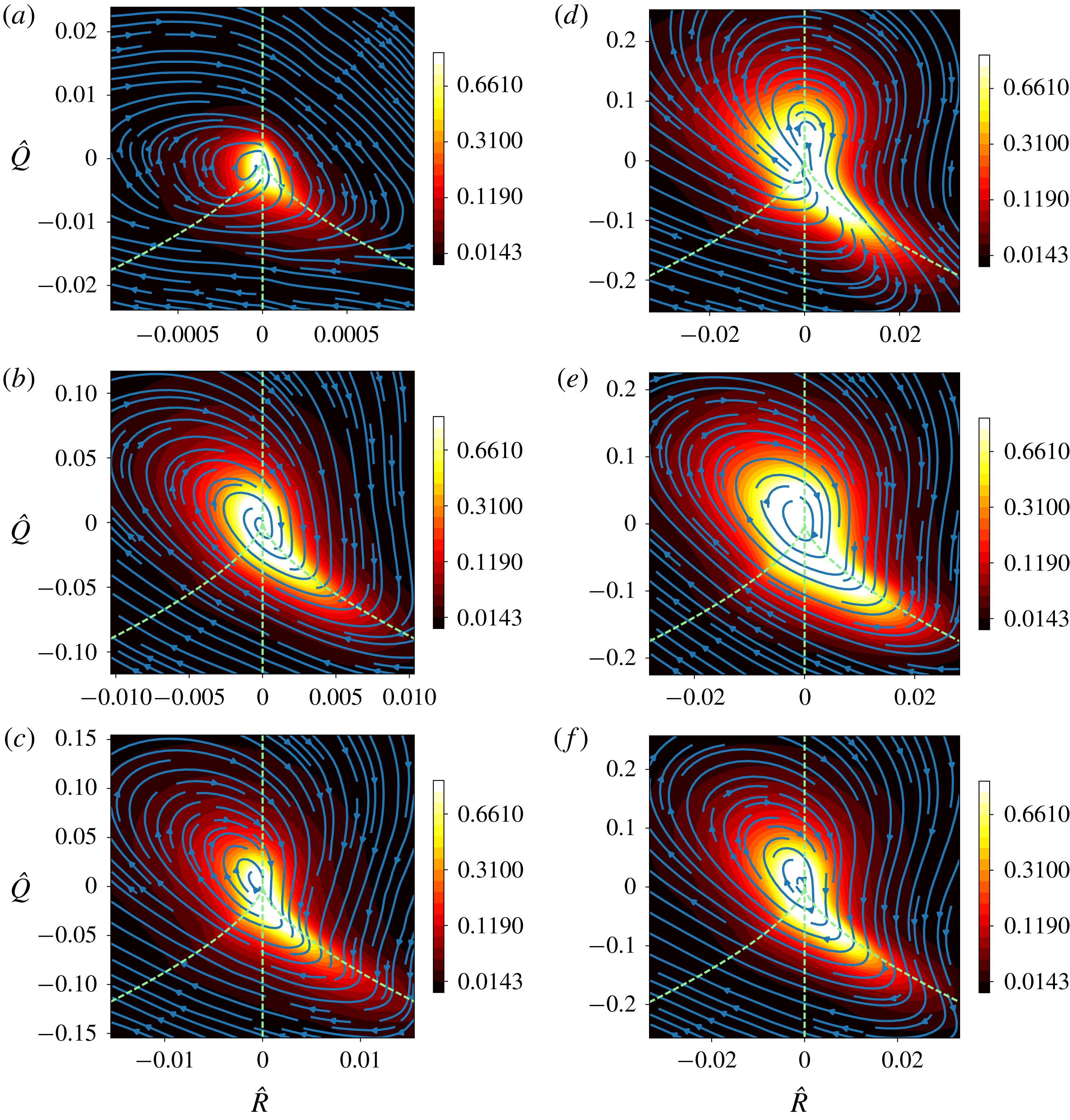
The mean
 $QR$
development with distance to the wall at the TE and near wake: (a–c) TE (
 $98\,\%$
chord); (d–f) near wake (
 $5\,\%$
chord from aerofoil TE). The dashed lines divide the
 $QR$
space into four sectors which cover, respectively, a certain flow topology as mentioned in § 1.

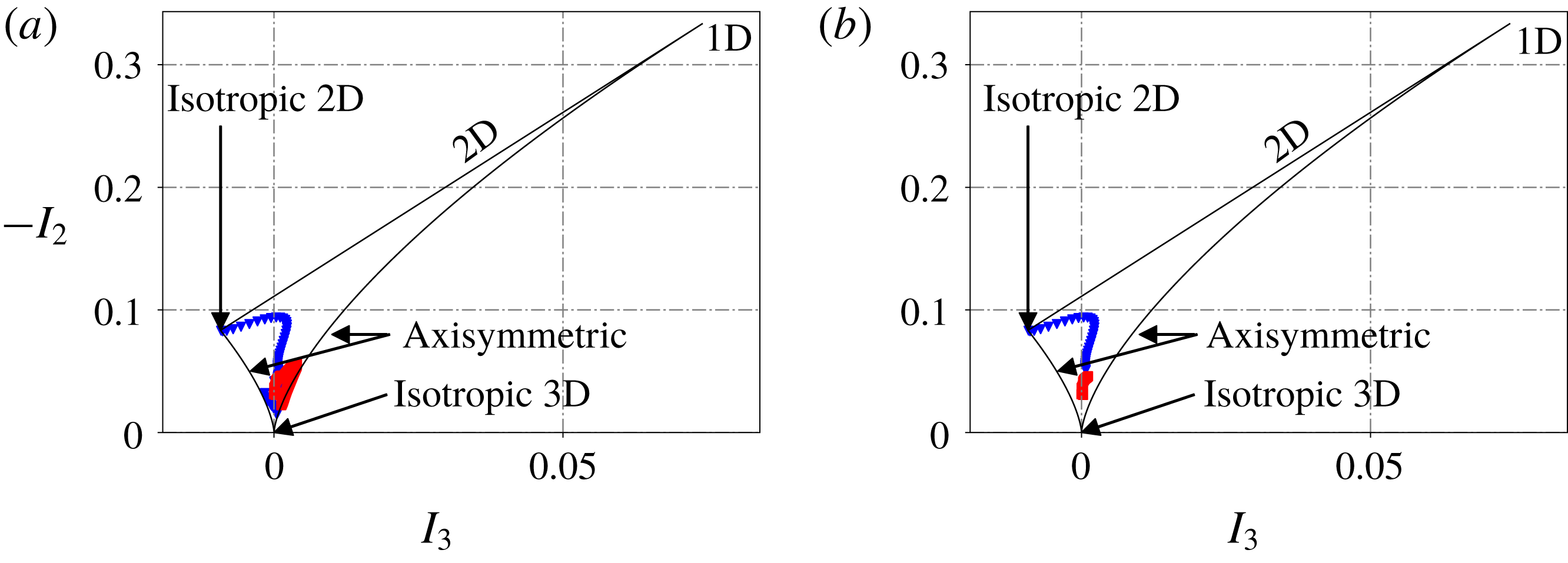
Anisotropy invariant map for locations at TE (98 % chord, ▴) and near wake (
 $x/c=0.05$
to TE, ▪): (a) entire boundary layer and (b) near-wall distribution up to
 $y^{+}\approx 6$
.

4.4 Effects of the wall: trailing-edge to near-wake flow development
As partly mentioned in the previous sections, the wall has significant effects on the overall
 $QR$
distribution when compared to HIT flows. This can already be seen from the comparison between the current flow over the aerofoil and HIT flow reported in the literature, as well as from the comparison between the flow near the aerofoil TE and the flow in the near wake. Figure 18 shows the flow at
 $98\,\%$
aerofoil chord and its adjacent area in the wake
 $5\,\%$
aerofoil chord downstream of the TE. More precisely, in figure 18, each row corresponds to regions in the boundary layer at TE and in the near wake (left to right) and each column corresponds to either of these two regions from near wall (or near the wake centreline) to locations further from wall (or further from the wake centreline) (top to bottom). The wall-normal locations in the boundary layer at
 $98\,\%$
aerofoil chord are
 $y^{+}\approx 6$
,
 $y^{+}\approx 24$
and
 $y^{+}\approx 180$
, respectively. From the horizontal comparisons (TE flow with their counterparts following the streamlines in the near wake), the
 $QR$
distribution in the near wake is clearly seen to be more isotropic: all locations exhibit a teardrop shape whereas the TE flow shows significant differences with varying tangential locations. In order to confirm and to quantify the difference in anisotropy levels, the anisotropy invariant map first introduced by Lumley (Reference Lumley1979) is used. Details about the application of such a tool can be found in Simonsen & Krogstad (Reference Simonsen and Krogstad2005) for instance. Figure 19 shows the distribution of the second and third invariants,
 $-I_{2}$
and
 $I_{3}$
, of the Reynolds stress tensor
 $\unicode[STIX]{x1D63C}_{Re}$
defined as
 $$\begin{eqnarray}\unicode[STIX]{x1D63C}_{Re}=\left[\begin{array}{@{}ccc@{}}\displaystyle \frac{\overline{\unicode[STIX]{x1D70C}u_{x}u_{x}}}{\overline{\unicode[STIX]{x1D70C}}}-\widetilde{u_{x}}\widetilde{u_{x}} & \displaystyle \frac{\overline{\unicode[STIX]{x1D70C}u_{x}u_{y}}}{\overline{\unicode[STIX]{x1D70C}}}-\widetilde{u_{x}}\widetilde{u_{y}} & \displaystyle \frac{\overline{\unicode[STIX]{x1D70C}u_{x}u_{z}}}{\overline{\unicode[STIX]{x1D70C}}}-\widetilde{u_{x}}\widetilde{u_{z}}\\[12.0pt] \displaystyle \frac{\overline{\unicode[STIX]{x1D70C}u_{y}u_{x}}}{\overline{\unicode[STIX]{x1D70C}}}-\widetilde{u_{y}}\widetilde{u_{x}} & \displaystyle \frac{\overline{\unicode[STIX]{x1D70C}u_{y}u_{y}}}{\overline{\unicode[STIX]{x1D70C}}}-\widetilde{u_{y}}\widetilde{u_{y}} & \displaystyle \frac{\overline{\unicode[STIX]{x1D70C}u_{y}u_{z}}}{\overline{\unicode[STIX]{x1D70C}}}-\widetilde{u_{y}}\widetilde{u_{z}}\\[12.0pt] \displaystyle \frac{\overline{\unicode[STIX]{x1D70C}u_{z}u_{x}}}{\overline{\unicode[STIX]{x1D70C}}}-\widetilde{u_{z}}\widetilde{u_{x}} & \displaystyle \frac{\overline{\unicode[STIX]{x1D70C}u_{z}u_{y}}}{\overline{\unicode[STIX]{x1D70C}}}-\widetilde{u_{z}}\widetilde{u_{y}} & \displaystyle \frac{\overline{\unicode[STIX]{x1D70C}u_{z}u_{z}}}{\overline{\unicode[STIX]{x1D70C}}}-\widetilde{u_{z}}\widetilde{u_{z}}\end{array}\right],\end{eqnarray}$$
where
 $x$
,
 $y$
and
 $z$
are the streamwise, vertical and spanwise directions, respectively. Invariants
 $I_{2}$
and
 $I_{3}$
are defined as
 $$\begin{eqnarray}\displaystyle & \displaystyle I_{2}={\textstyle \frac{1}{2}}(\text{trace}(\unicode[STIX]{x1D63C}_{Re})^{2}-\text{trace}(\unicode[STIX]{x1D63C}_{Re}^{2})), & \displaystyle\end{eqnarray}$$
 $$\begin{eqnarray}\displaystyle & \displaystyle I_{3}=\text{det}(\unicode[STIX]{x1D63C}_{Re}). & \displaystyle\end{eqnarray}$$
In figure 19(a), the distribution of the anisotropy level of wall-normal points from the wall to the edge of the boundary layer (up to
 $\unicode[STIX]{x1D6FF}_{p99}$
) at the TE (98 % chord) and their counterparts in the near wake (
 $x/c=0.05$
to TE) again clearly shows that, in the absence of the wall, the turbulence becomes more isotropic as the values of
 $I_{3}$
and
 $-I_{2}$
from the points in the near wake are much closer to the 3D isotropic point where
 $I_{3}$
and
 $-I_{2}$
tend to zero. In figure 19(b), it can be seen that the most severe departure from the 3D isotropy for TE points in figure 19(a) is from the locations closer to the wall (from wall to
 $y^{+}\approx 6$
) as only the distribution of these near-wall points is plotted in this figure. These near-wall points have a nearly 2D isotropic behaviour. These plots thus further confirm that the trend seen in figures 18(a) and 18(d) comes from the fact that the flow becomes more isotropic in the absence of the aerofoil surface. Furthermore, the comparison between figures 18(a) and 18(d) shows that the wall greatly suppresses the vortical stretching character of the flow as the upper-left part of the
 $QR$
plot in the near wake is much bigger and rounder than that from the TE.
Another aspect worth mentioning, independent of all the flow conditions, is that, for all the investigated regions over the aerofoil and the near wake, the general mean life cycle of turbulent structures stays unchanged in the
 $QR$
space. This cycle starts from straining structures and develops to stretching vortical structures and further to contracting vortical structures before the life cycle continues again in the straining structures. This appears to be an invariant character for all the regions in the current flow under consideration.
5 Conclusion
With the weakly compressible Lagrangian dynamics of the two invariants of the velocity-gradient tensor,
 $Q$
and
 $R$
, the evolution of characteristic structures has been studied for the turbulent boundary layer on a controlled-diffusion (CD) aerofoil at chord-based Reynolds number of
 $Re_{c}=150\,000$
and a free-stream Mach number of
 $M=0.25$
at
 $8^{\circ }$
angle of attack. The quality of the simulation was carefully checked and it was ascertained that it properly reproduces the experimental results. The focus in the current work was on the changes of the evolution of the velocity-gradient tensor invariant dynamics related to pressure gradient for different wall-normal locations of the flow.
The mean profiles from the turbulent boundary layer at different chordwise positions suggest that pressure gradient greatly changes the topology of the boundary layer. Compared with ZPG condition, an APG acts as a reinforcement of the intense momentum exchange by fluctuating velocities, which is extended from the viscous sublayer to the log layer and even to the edge of the outer layer. This gradient leads to a platform shape for wall-parallel Reynolds stress components and a hump shape connected by two peak values of turbulence production terms.
The mean evolution of the velocity-gradient tensor invariant dynamics was found to vary strongly for regions undergoing FPG, ZPG and APG. The shape of the
 $QR$
plots of the log layer and the outer layer strongly depends on the mean local pressure gradients while the viscous sublayer has an invariant character: oval shape independent of the pressure-gradient conditions. Furthermore, this evolution also changes greatly with the distance to the wall. Key changes are explained in the context of
 $QR$
plots with mean trajectories and as well from mean profiles giving both outer and inner scale as reference.
The role of nonlinearity and viscous diffusion in the overall evolution of the velocity-gradient tensor invariant dynamics maintain their respective invariant characteristic for all investigated regions regardless of the different pressure-gradient conditions. The nonlinearity drives the global shape of the
 $QR$
plots. The viscous diffusion drives all structures towards the origin. These two aspects thus do not appear to be the major reasons for the changes of the turbulence evolution for the different investigated regions.
In fact, the coupling of the pressure Hessian with the velocity gradient, which is strongly affected by the mean pressure-gradient conditions and the wall, is the major factor that drives all the changes of the invariant dynamics in this flow. From a
 $QR$
space analysis point of view, this coupling seems to be the most significant feature that affects the turbulence development and is highly influenced by the local mean pressure gradient and wall-normal distance. The comparison between previous ZPG turbulent boundary layer data and the results from FPG and APG regions in this aerofoil flow shows that the pressure gradients have a significant impact at least in the outer layer and log layer of the flow. The APG leads to more rolling features to the mean trajectories in these two layers and suppresses the vortical stretching regime.
The wall effects are contrasted with previous studies, and a comparison between the TE flow and the flow in the near wake is also provided. The wall is observed to mainly suppress the vortical stretching features of the flow and the flow exhibits a uniform feature in
 $QR$
space, known as a teardrop in the absence of the wall.
Lastly, despite different flow conditions for the investigated regions from the current flow case, the general mean life cycle of turbulent structures stays unchanged in
 $QR$
space.
Acknowledgements
This work is financed by an NSERC Discovery Grant of Canada. The computations are performed on the supercomputers Mammoth-MP2 at Université de Sherbrooke and Guillimin at McGill University, managed by Calcul Québec and Compute Canada. Special thanks go to Dr P. Bechlars from MTU Aero Engines AG and Professor X. Wu from Royal Military College of Canada for helpful discussions on this topic and their precious advice.