1 Introduction and motivation
Modelling dependence structures in stochastic processes is a rather difficult task. Therefore, most stochastic models start under the restrictive assumption having independence between different risk factors, different risk modules, different portfolios, different accident years, etc. This is a common situation in general insurance claims run-off modelling where one usually assumes that claims payments of different accident years are independent (see, for instance, Mack (Reference Mack1993) and Hertig (Reference Hertig1985)). Under these independence assumptions, predictors and corresponding confidence bounds are derived. Of course, one is aware of the fact that positive correlation widens these confidence bounds due to less diversification benefits. Therefore, as a next (and final) step practitioners do a “top level” correlation correction by simply multiplying the confidence bounds (obtained from the independent case) with a deterministic factor.
In the present paper we derive a comprehensive bottom-up approach for dependence modelling in general insurance claims run-offs. We choose a particular multivariate log-normal chain-ladder model and in this model we derive predictors and confidence bounds in closed form. These analytical solutions are such that they allow for any correlation structure. From this we can then analyze the quality of the top level correlation corrections done by practitioners. Moreover, we can calibrate correlation for risk management models which is still an open issue in Solvency 2, see European Commission (2010) and Swiss Solvency Test (2006).
There are only a few related results in the literature. Basically, there are three streams of literature on dependence modelling in general insurance claims run-offs:
(1) Claims inflation and accounting year dependence within a claims run-off triangle. The first source of dependence that has been identified by practitioners is claims inflation within a run-off triangle which acts on all accident years simultaneously. The classical distribution-free chain-ladder model of Mack (Reference Mack1993) cannot cope with this form of dependence. First papers that study this form of dependence are Barnett & Zehnwirth (Reference Barnett and Zehnwirth2000), Brehm (Reference Brehm2002), de Jong (Reference de Jong2006), Kirschner et al. (Reference Kirschner, Kerley and Isaacs2008), Kuang et al. (Reference Kuang, Nielsen and Nielsen2008), Shi et al. (Reference Shi, Basu and Meyers2012) and Wüthrich (Reference Wüthrich2010). The first five papers mainly study this form of dependence using either maximum-likelihood methods or bootstrap simulation methods. The last two papers study accounting year dependence in a Bayesian inference framework using Markov chain Monte Carlo simulation methods. The present paper extends and combines the model and the ideas of de Jong (Reference de Jong2006) (which goes back to Hertig (Reference Hertig1985)) and the Bayesian inference framework studied in Shi et al. (Reference Shi, Basu and Meyers2012) and Wüthrich (Reference Wüthrich2010). This combination is done such that we are able to derive analytical results which allow to analyze prediction uncertainty for solvency purposes.
(2) Cell-wise dependence between run-off triangles. A second stream of literature studies the aggregation of different claims reserving triangles (sub-portfolios), see Braun (Reference Braun2004), Merz & Wüthrich (Reference Merz and Wüthrich2007, Reference Merz and Wüthrich2008a), Shi & Frees (Reference Shi and Frees2011) and Zhang et al. (Reference Zhang, Dukic and Guszcza2012). These papers study a cell-wise dependence between different run-off triangles (sub-portfolios). Our model will also allow to model this form of dependence. It will turn out that this form of cell-wise dependence is a rather weak one compared to accounting year dependence.
(3) Combination of cell-wise dependence between and accounting year dependence within run-off triangles. The third stream of literature combines (1) and (2). Probably the first two papers that look at both forms of dependence in a rigorous mathematical way are Shi et al. (Reference Shi, Basu and Meyers2012) and Zhang et al. (Reference Zhang, Dukic and Guszcza2012). The former develops the modelling framework using a Bayesian methodology, whereas the latter describes inflation modelling in the concluding discussion. The present paper is in the spirit of Shi et al. (Reference Shi, Basu and Meyers2012). Shi et al. (Reference Shi, Basu and Meyers2012) use an additive model for incremental payments where dependence is modelled in two directions (accident year and accounting year). The accounting year dependence modelling in Shi et al. (Reference Shi, Basu and Meyers2012) can be interpreted as a hierarchical structure which leads to a new interesting family of models related to hierarchical generalized linear models (HGLM), see Gigante et al. (Reference Gigante, Picech and Sigalotti2012).
The starting point of our model is Hertig's log-normal chain-ladder model. We embed this multiplicative claims reserving model into a multivariate log-normal framework. This multivariate framework is chosen such that we can simultaneously model several claims run-off triangles (sub-portfolios). In this model we can choose any correlation structure between the sub-portfolios and also within the sub-portfolios. Parameter uncertainty is modelled with a multivariate Gaussian prior distribution (which is a conjugate prior to the multivariate log-normal distribution, see Bühlmann & Gisler (Reference Bühlmann and Gisler2005)). This combination then allows to give a closed form solution for the claims reserving problem. Moreover, it allows to derive closed form confidence bounds which, at the same time, study process uncertainty and parameter uncertainty. These results are then used to study sensitivities and, moreover, they can be used to calibrate correlation estimates for solvency purposes.
The nature of our multiplicative model and of the additive model of Shi et al. (Reference Shi, Basu and Meyers2012) is such that they allow to utilize mathematical properties of multivariate Gaussian structures (leading to closed form solutions). The main weakness of these models is that they use a multivariate Gaussian copula as dependence structure. This dependence structure does not enjoy tail dependence (see McNeil et al. (Reference McNeil, Frey and Embrechts2005)) and therefore joint extremes are probably under-estimated, this is also stated in Shi & Frees (Reference Shi and Frees2011). Moreover, often the log-normal distribution is not sufficiently heavy-tailed for modelling the tails of extremes. However, analytical formulas can only be found under these assumptions and their generalization will require simulations. Therefore, our model can serve as a benchmark for more evolved simulation-based methods. Moreover, we would like to highlight that we get fundamental findings from our model (see Conclusions 1–5 below) which explain that the state-of-the-art handling of correlation in practice should be changed, because correlation is often under-estimated (and mis-specified).
Organization of the paper. In the next section we define the multivariate Bayesian claims reserving model. In Section 3 we describe the prediction problem from a general point of view in our modelling framework. The surprisingly simple Theorem 3.1 is the key result that paves the way for closed form solutions. In Section 4 we adapt the notion from the previous section to claims reserving triangles. In Section 5 we describe the claims development result which is a crucial risk factor in Solvency 2 and we analyze prediction uncertainty in this balance sheet position. Finally, in Section 6 we present an extended case study which results in several conclusions summarized in Section 7. All proofs are provided in the appendix.
2 Model assumptions
Accident years are denoted by i∈{1,…,I} and development years by j∈{0,…, J}. We assume that I ≥ J + 1 and that all claims are settled after development year J. Cumulative claims are denoted by Ci,j,n > 0, where the last index n∈{1,…,N} corresponds to the n-th sub-portfolio (or line of business). We define the individual log-link ratios  $$)(-->$<>\xi<$>
<!--$$i,j,n by (set
 $$)(-->$<> {{C}_{i,{\rm{ - }}1,n}}\: \equiv \:1 <$>
<!--$$ for all i and n)
 $${{\xi }_{i,j,n}}\: = \:{\rm{log}}\left( {{{C}_{i,j,n}}/{{C}_{i,j{\rm{ - }}1,n}}} \right) \ \ \Leftrightarrow\ \ {{C}_{i,j,n}}\: = \:{{C}_{i,j{\rm{ - }}1,n}}{\rm{exp}}\left\{ {{{\xi }_{i,j,n}}} \right\}.$$
We stack the random variables  $$)(-->$<>\xi<$>
<!--$$i,j,n into random vectors which will provide a handy notation. For i∈{1,…,I} and j∈{0,…,J} we define the vectors
 $$)(-->$<> {{\xi }_{i,j}}\: = \:({{\xi }_{i,j,1}}, \ldots, {{\xi }_{i,j,N}})^{\prime} \!\in {{{\Bbb R}}^N}, \ {{{\bf {{\bixi }}}}_i}\: = \:(\xi {{^{\prime}}_{i,0}}, \ldots, \xi {{^{\prime}}_{i,J}})^{\prime}\in {{{\Bbb R}}^a} <$>
<!--$$ and
 $$)(-->$<> \bixi \: = \:({\bf {{\bixi }}}_1{{^{\prime}}}, \ldots, {\bf {{\bixi }}}_I{{^{\prime}}})^{\prime}\in {{{\Bbb R}}^d} <$>
<!--$$, with a = N(J + 1) and d = aI.
Remarks.
• The multiplicative structure (2.1) in the development period j will imply that we have a chain-ladder type model, see Mack (Reference Mack1993).
• The parameter n∈{1,…,N} denotes the sub-portfolios (or different lines of business). If we have only one sub-portfolio, i.e. N = 1, then we set
 $$)(-->$<>\xi<$>
<!--$$i,j,n = $$)(-->$<>\xi<$>
<!--$$i,j and we are in the classical one-dimensional claims reserving problem.
• Under the assumptions that N = 1 and that the
$$)(-->$<>\bixi<$>
<!--$$i,j 's are independent Gaussian distributed with mean θ j we are in the framework of Hertig's log-normal claims reserving model, see Hertig (Reference Hertig1985). Our aim is to relax these independence assumptions and to extend the model to N > 1.


Model Assumptions 2.1 (multivariate log-normal claims reserving model)
• Conditionally, given parameter
$$)(-->$<> {\bf {{\brTheta }}}\, \in \,{{{\Bbb R}}^a} <$>
<!--$$, the random vector $$)(-->$<>\bixi<$>
<!--$$ has a multivariate Gaussian distribution with fixed positive-definite covariance matrix $$)(-->$<> {\rm{\rSigma }}\, \in \,{{{\Bbb R}}^{d\,\times \,d}} <$>
<!--$$ and conditional expected values$$)(-->$<> {\Bbb E}\left[ {\left. {{{\bixi }_i}} \right|{\bf {{\brTheta }}}} \right]\, = \,{\bf {{\brTheta }}},\; \; \; \; {\rm{for}}\;{\rm{all}}\,i\, \in \,{\rm{\{ 1,}} \ldots {\rm{,}}I{\rm{\} }} <$>
<!--$$.• The parameter Θ has a multivariate Gaussian distribution with prior mean
$$)(-->$<> \bimu \, \in \,{{{\Bbb R}}^a} <$>
<!--$$ and positive-definite prior covariance matrix $$)(-->$<> T\, \in \,{{{\Bbb R}}^{a\,\times \,a}} <$>
<!--$$.


□
Often it is easier to describe the model assumptions by simply writing down the density function. Under Model Assumptions 2.1, the joint density of  $$)(-->$<>\bixi<$>
<!--$$ and Θ at position (
 $$)(-->$<>\bixi<$>
<!--$$,θ) is given by
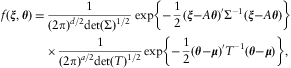 $${ f(\bixi, \bitheta )\: = \:\,\frac{1}{{{{{(2\pi )}}^{d/2}} {\rm{d}}{\rm et}{{{(\rSigma )}}^{1/2}} }} \,{\rm{exp}}\left\{ {{\rm{ - }}\frac{1}{2}\left( {\bixi {\rm{ - }}A\bitheta } \right)^{\prime}{{\rSigma }^{{\rm{ - }}1}} \left( {\bixi {\rm{ - }}A\bitheta } \right)} \right\} \cr & \times \: \frac{1}{{{{{(2\pi )}}^{a/2}} {\rm{det}}{{{(T)}}^{1/2}} }} {\rm{exp}}\left\{ {{\rm{ - }}\frac{1}{2}\left( {\bitheta {\rm{ - }}\bimu } \right)^{\prime}{{T}^{{\rm{ - }}1}} \left( {\bitheta {\rm{ - }}\bimu } \right)} \right\}, \cr}$$
with matrix  $$)(-->$<> A\: = \:(\tf="Casopfan-R" 1, \ldots, \tf="Casopfan-R" 1)^{\prime} \in {{{\Bbb R}^{\tf="Sabon_I" {d\,\times \,a}} <$>
<!--$$ consisting of I = d/a identity matrices denoted by
 $$)(-->$<> {\tf="Casopfan-R" 1}\: \in \:{{{\Bbb R}}^{a\times a}} <$>
<!--$$ and describing the conditional mean
 $$)(-->$<> {\tf="Casopfan-R" E}\left[ {\bixi \:|\:{\bf {{\brTheta }}}} \right]\: = \:A{\bf {{\brTheta }}}\: = \:({\bf {{\brTheta }}}^{\prime}, \ldots, {\bf {{\brTheta }}}^{\prime})^{\prime}\: \in \:{{{\Bbb R}}^d} <$>
<!--$$.
Remarks 2.2
• We choose a multivariate Gaussian model for the individual log-link ratios
$$)(-->$<>\xi<$>
<!--$$i,j,n which gives log-normal distributions for cumulative claims Ci,j,n. For risk management and solvency purposes one might argue that this is not a sufficiently heavy-tailed model and, moreover, this model does not have tail dependence. Nevertheless, we believe that the results from this model are interesting and important also on their own and that our model may serve as a benchmark for the ad-hoc methods used in practice and for more complex multivariate extreme value models (which still need to be developed in this field and which, in general, can only be solved numerically, for instance, using Markov chain Monte Carlo simulation methods).• The covariance matrix
$$)(-->$<>\rSigma<$>
<!--$$ will allow for any correlation structure between the individual log-link ratios $$)(-->$<>\xi<$>
<!--$$i,j,n such as accounting year dependence or dependence between different sub-portfolios n. We provide explicit choices in Section 6 below.• Parameter uncertainty is modelled through the choice of a prior distribution for Θ. Thus, a Bayesian inference analysis will include parameter estimation uncertainty in a natural way through posterior distributions.
• The model assumptions imply that conditionally, given Θ,
$${{C}_{1,0,n}}\: = \:{\rm{exp}}\{ {{\xi }_{1,0,n}}\}, \; \ldots, {{C}_{I,0,n}}\: = \:{\rm{exp}}\{ {{\xi }_{I,0,n}}\} \; \; {\rm{are}}\;{\rm{identically}}\;{\rm{distributed}}{\rm{.}}$$That is, there is no specific accident year i∈{1,…,I} parameter under Model Assumptions 2.1. This model assumption can easily be relaxed if it is not appropriate in a particular situation. There are several different possibilities to do so, for instance
(1) if there are known prior differences, choose suitable constants for
$$)(-->$<> {{C}_{i,{\rm{ - }}1,n}}\: = \:{{\nu }_{i,n}}\: \in \:{{{\Bbb R}}_ + } <$>
<!--$$ which give multiplicative prior adjustments, i.e. $$)(-->$<> {{C}_{i,0,n}}\: = \:{{\nu }_{i,n}}{\rm{exp}}\{ {{\xi }_{i,0,n}}\} <$>
<!--$$;(2) a second way extends
$$)(-->$<> {{\xi }_{i,0,n}}\: = \:\xi _{{i,0,n}}^{{(1)}} \: + \:\xi _{{i,0,n}}^{{(2)}} <$>
<!--$$ to a bivariate term with $$)(-->$<> \xi _{{i,0,n}}^{{(1)}} <$>
<!--$$ similar to (2.3) and independent Gaussian random variables $$)(-->$<> \xi _{{i,0,n}}^{{(2)}} <$>
<!--$$ reflecting differences between accident years i;(3) or define the model conditional on the first columns, i.e. given Ci ,0,n for all i and n.








All these proposals lead to closed form solutions.
In our analysis we will calculate posterior distributions given observations in the upper claims reserving triangle Dt, t ≥ I, see (4.1) and (4.2) below. This will imply that the exposure of accident year i is always proportional to the last observation of accident year i at time t, i.e. proportional to Ci ,t −i ,n, see Theorem 4.1. This is rather close to option (3) from above and the restrictive assumption (2.3) only influences parameter estimation. Therefore, we refrain from increasing the complexity of our model.
• Crucial for the closed form solution is the multivariate Gaussian structure (2.2) which is the key property to all results in the next section. This is similar to the results in the additive model of Shi et al. (Reference Shi, Basu and Meyers2012), formulas (1)–(4). Relaxation of this assumption may lead to hierarchical generalized linear models (HGLM) as they are used, for instance, in Gigante et al. (Reference Gigante, Picech and Sigalotti2012). However, many of the analytical properties get lost in these more complex models and either simulations or approximations need to be used.
• The model can be generalized to sub-portfolios n all having different dimensions I and J. The analysis will be the same but the notation will become more cumbersome, therefore we refrain from doing so.
3 Unconditional and predictive distributions
The Bayesian Model Assumptions 2.1 describe the distribution of  $$)(-->$<>\bixi<$>
<!--$$, given the parameter Θ. Since, in general, this parameter is not known experts specify a prior distribution for it. In classical credibility theory one then collects observations
 $$)(-->$<>\xi<$>
<!--$$i,j,n and calculates the posterior distribution of Θ, given these observations, see e.g. Bühlmann & Gisler (Reference Bühlmann and Gisler2005). In the present situation it is simpler to directly work with the unconditional distribution of
 $$)(-->$<>\bixi<$>
<!--$$. That is, though we have a classical Bayesian model including parameter uncertainty, we do not describe the posterior distribution of the parameter Θ explicitly, but we directly work on the data having the parameter distribution of Θ as a latent factor (this can be done because the parameter Θ acts in a simple way as a location parameter as the third proof of Theorem 3.1 will show). Thus, in a first step we calculate the unconditional distribution of
 $$)(-->$<>\bixi<$>
<!--$$, and in a second step we calculate the predictive distribution of
 $$)(-->$<>\bixi<$>
<!--$$ if we observe some of its components
 $$)(-->$<>\bixi<$>
<!--$$i,j,n.
Theorem 3.1 (unconditional distribution)Under Model Assumptions 2.1 the random vector  $$)(-->$<>\bixi<$>
<!--$$has a multivariate Gaussian distribution with the first two moments given by
 $$ {\Bbb E}\left[ \bixi \right]\: = \:A\bimu \; \; \;{and}}\;\; \; S\: = \:{\rm{Cov}}\left( \bixi \right)\: = \:\rSigma \: + \:ATA^{\prime}. $$
In the proof of Theorem 3.1 we derive the following (side-)result for the covariance matrix S.
Corollary 3.2 Under Model Assumptions 2.1 we have for the covariance matrix S =  $$)(-->$<>\rSigma<$>
<!--$$ + ATA′
 $${{S}^{{\rm{ - }}1}} \: = \:{{{\rm{\rSigma }}}^{{\rm{ - }}1}} {\rm{ - }}{{{\rm{\rSigma }}}^{{\rm{ - }}1}} A{{(A^{\prime}{{{\rm{\rSigma }}}^{{\rm{ - }}1}} A\: + \:{{T}^{{\rm{ - }}1}} )}^{{\rm{ - }}1}} A^{\prime}{{{\rm{\rSigma }}}^{{\rm{ - }}1}} .$$
Next our aim is to describe the distribution of  $$)(-->$<>\bixi<$>
<!--$$ if we have observed some of its components
 $$)(-->$<>\bixi<$>
<!--$$i,j,n. We choose a non-empty, real subset
 $${\scr D}\: \subset \:\{ (i,j,n); \ {i = \:1, \ldots, I,\ j\: = \:0, \ldots, J,\,n\: = \:1, \ldots, N\} {\mathop{ = }\limits^{{{\rm{d}}\rm ef.}}} {\scr J},$$
i.e.  $$)(-->$<> {\scr D}\, \notin \,\{ {\scr J},\varnothing \} <$>
<!--$$. Let
 $$)(-->$<> |{\scr D}| <$>
<!--$$ denote the cardinality of
 $$)(-->$<> {\scr D} <$>
<!--$$. Define
 $$)(-->$<> {{P}_{\scr D}} <$>
<!--$$ to be the projection
 $$)(-->$<> {{{\Bbb R}}^d} \: \rightarrow \:{{{\Bbb R}}^{\cal|D|}} <$>
<!--$$ onto the components
 $$)(-->$<> (i,j,n)\, \in \,{\scr D} <$>
<!--$$, that is,
 $$\bixi \ \mapsto \ {{\bixi }^{\scr D}} \: = \:{{P}_{\scr D}}\bixi, $$
such that  $$)(-->$<> {{{\rm{\bixi }}}^{\scr D}} <$>
<!--$$ exactly contains the components of
 $$)(-->$<>\bixi<$>
<!--$$ which are in
 $$)(-->$<> {\scr D} <$>
<!--$$. Analogously,
 $$)(-->$<> {{P}_{{{{\scr D}}^c} }} <$>
<!--$$ denotes the projection onto the components in the complement
 $$)(-->$<>{{{\scr D}}^c} \, = \,{\scr J}{\backslash}{\scr D} <$>
<!--$$ of
 $$)(-->$<> {\scr D} <$>
<!--$$ and
 $$)(-->$<> {{\bixi }^{{{{\scr D}}^c} }} <$>
<!--$$ denotes the corresponding components. Thus, we consider the (bijective) decomposition
 $$\bixi \ \mapsto \ ({{\bixi }^{\scr D}}, {{\bixi }^{{{{\scr D}}^c} }} )$$
which separates  $$)(-->$<> {{{\Bbb R}}^d} <$>
<!--$$ into two disjoint (non-empty) subspaces
 $$)(-->$<> {{{\Bbb R}}^{{\scr |D|}}} <$>
<!--$$ and
 $$)(-->$<> {{{\Bbb R}}^{|{{{\scr D}}^c} |}} <$>
<!--$$. Our aim is to predict
 $$)(-->$<> {{\bixi }^{{{{\scr D}}^c} }} <$>
<!--$$ when we have observed
 $$)(-->$<> {{\bixi }^{\scr D}} <$>
<!--$$.
Lemma 3.3 Under Model Assumptions 2.1 the random vector  $$)(-->$<>({{\bixi }^{\scr D}}, {{\bixi }^{{{{\scr D}}^c} }} )<$>
<!--$$has a multivariate Gaussian distribution with the first two moments given by
 $${ {{\bimu }_{\cal D}}\: = & \:{\Bbb E}\left[ {{{\bixi }^{\scr D}} } \right]\: = \:{{P}_{\scr D}}\,A\bimu \; \; \ \ \ \ {{and}}\; \; \ \ \ \ {{S}_{\scr D}}\: = \:{\rm{Cov}}\left( {{{\bixi }^{\scr D}} } \right)\: = \:{{P}_{\scr D}}SP{{^{\prime}}_{\scr D}}, \cr {{\bimu }_{{{\cal D}^c} }}\: = & \:{\Bbb E}\left[ {{{\bixi }^{{{{\scr D}}^c} }} } \right]\: = \:{{P}_{{{{\scr D}}^c} }}\,A\bimu \; \; \ \ \ \ {{and}}\; \; \ \ \ \ {{S}_{{{{\scr D}}^c} }}\: = \:{\rm{Cov}}\left( {{{\bixi }^{{{{\scr D}}^c} }} } \right)\: = \:{{P}_{{{{\scr D}}^c} }}SP{{^{\prime}}_{{{{\scr D}}^c} }}. \cr}$$
The covariance matrix between the components  $$)(-->$<> {{\bixi }^{\scr D}} <$>
<!--$$and
 $$)(-->$<> {{\bixi }^{{{{\scr D}}^c} }} <$>
<!--$$is given by
 $${{S^{\prime}}_{{{{\scr D}}^c}, {\scr D}}}\: = \:{{S}_{{\scr D},{{{\scr D}}^c} }}\: = \:{\rm{Cov}}\left( {{{\bixi }^{\scr D}}, {{\bixi }^{{{{\scr D}}^c} }} } \right)\: = \:{{P}_{\scr D}}SP{{^{\prime}}_{{{{\scr D}}^c} }}.$$
Note that Cov( $$)(-->$<>\bixi<$>
<!--$$) (with one argument) denotes the covariance matrix of the random vector
 $$)(-->$<>\bixi<$>
<!--$$, and, by a slight abuse of notation, we denote by Cov(
 $$)(-->$<>\bixi<$>
<!--$$,η) (with two arguments) the covariance matrix between the two random vectors
 $$)(-->$<>\bixi<$>
<!--$$ and η. We are now ready to give the crucial statement providing the predictive distribution of
 $$)(-->$<> {{\bixi }^{{{{\scr D}}^c} }} <$>
<!--$$, conditionally given observations
 $$)(-->$<> {{\bixi }^{\scr D}} <$>
<!--$$.
Theorem 3.4 (predictive distribution)Under Model Assumptions 2.1 we have the following statement: the conditional distribution of  $$)(-->$<> {{\bixi }^{{{{\scr D}}^c} }} <$>
<!--$$, given
 $$)(-->$<>{{\bixi }^{\scr D}} <$>
<!--$$, is a multivariate Gaussian distribution with conditional mean given by
 $$\bimu _{{{{{\scr D}}^c} }}^{{{\rm{post}}}} \: = \:{\Bbb E}\left[ {\left. {{{\bixi }^{{{{\scr D}}^c} }} } \right|{{\bixi }^{\scr D}} } \right]\: = \:{{\bimu }_{{{{\scr D}}^c} }}\: + \:{{S}_{{{{\scr D}}^c}, {\scr D}}} {{\left( {{{S}_{\scr D}}} \right)}^{{\rm{ - }}1}} \left( {{{\bixi }^{\scr D}} {\rm{ - }}{{\bimu }_{\scr D}}} \right),$$
and conditional covariance matrix given by
 $$S_{{{{\scr D}^c} }}^{{{\rm{p}}ost}} \: = \:{\rm{Cov}}\left( {\left. {{{{\bf {{\bixi }}}}^{{{\scr D}^c} }} } \right|{{{\bf {{\bixi }}}}^{\scr D}} } \right)\: = \:{{S}_{{{\scr D}^c} }}{\rm{ - }}{{S}_{{{\scr D}^c}, {\scr D}} {{\left( {{{S}_{\scr D}} \right)}^{{\rm{ - }}1}} {{S}_{{{\scr D}}, {\scr D}^c}.$$
4 Ultimate claim prediction and prediction uncertainty
We apply Theorem 3.4 to the claims reserving problem. Assume that we are at time t ≥ I (with t < I + J). Then, we have observed the cumulative claims Ci ,j ,n with i + j ≤ t. Note that we choose t ≥ I to ensure that the first column {(i,j,n); 1 ≤i ≤ I, j = 0} of each claims development triangle n∈{0,…,N} has been observed. Thus, the data is determined by the indices
 $${{\scr D}_t}\: = \:\left\{ {(i,j,n)\: \in \:{\scr J}}; i\: + \:j\:\leq \:t} \right\},$$
and the resulting σ-field at time t is given by
 $${{\scr F}_t}{\mathop{ = }\limits^{{{\rm{def}}{\rm{.}}}}} \sigma \left\{ {{{C}_{i,j,n}};\,(i,j,n)\: \in \:{{\scr D}_t}} \right\}\: = \:\sigma \left\{ {{{\bixi }_{i,j,n}}; (i,j,n)\: \in \:{{\scr D}_t}} \right\}\: = \:\sigma \left\{ {{{\bixi }^{{{\scr D}_t}}} } \right\}.$$
The Bayesian predictor for the ultimate claim Ci ,J ,n, i ≥ t−J + 1, at time t ≥ I is given by
 $${\mathop{\widehat C}\nolimits^{}} _{{i,J,n}}^{{(t)}} \: = \:{\Bbb E}\left[ {\left. {{{C}_{i,J,n}}} \right|{{\scr F}_t}} \right]\: = \:{{C}_{i,t{\rm{ - }}i,n}} {\Bbb E}\left[ {\left. {{\rm{exp}}\left\{ {\mathop{\sum}\limits_{j\: = \:t{\rm{ - }}i\: + \:1}^J {{\bixi }_{i,j,n}}} \right\}} \right|{{\bixi }^{{{{\scr D}}_t}}} } \right].$$
Assume that 1≤t−i + 1≤J. Then we can define the set of indices
 $${\scr D}_{{t|i,n}}^{c} \: = \:{\scr D}_{t}^{c} \: \cap \:\left\{ {(l,j,m)\: \in \:{\scr J};\,l\: = \:i,\,m\: = \:n} \right\},$$
which provides the projection  $$)(-->$<> {{P}_{{\scr D}_{{t|i,n}}^{c} }}:{{{\Bbb R}}^d} \: \rightarrow \:{{{\Bbb R}}^{J{\rm{ - }}(t{\rm{ - }}i)}} <$>
<!--$$. Thus, we have
 $${\bf {{e}}}{{^{\prime}}_{t|i,n}}\,{{{\bf {{\bixi }}}}^{{\scr D}_{t}^{c} }} {\mathop{ \ \ =\ \,\ }\limits^{{{\rm{def}}{\rm{.}}}}} (1, \ldots, 1)^{\prime} {{P}_{{\scr D}_{{t|i,n}}^{c} }}\bixi \: = \:\mathop{\sum}\limits_{j\: = \:t{\rm{ - }}i\: + \:1}^J {{\bixi }_{i,j,n}}.$$
Note that this sum exactly considers all un-observed components of  $$)(-->$<> {{\bixi }^{{\scr D}_{t}^{c} }} <$>
<!--$$ for a given accident year i and a given sub-portfolio n.
Theorem 4.1 (ultimate claim prediction)Under Model Assumptions 2.1 the ultimate claim predictor  $$)(-->$<>{\mathop{\widehat C}\nolimits^{}} _{{i,J,n}}^{{(t)}} <$>
<!--$$of sub-portfolio n∈{0,…,N} and accident year i∈{t−J + 1,…,I} is at accounting year t∈{I,…,I + J−1} given by
 $${\mathop{\widehat C}\nolimits^{}} _{{i,J,n}}^{{(t)}} \: = \:{{C}_{i,t{\rm{ - }}i,n}}\,{\rm exp}\left\{ {{{{\bf {{e}}}}^ {\prime}_{t|i,n}}\,{{\bf {{\bimu }}}_{{{\scr D}_{t}^{c} }}^{{{\rm{post}}}} \: + \:\frac{1}{2}\,{{{\bf {{e}}}}^{\prime}_{t|i,n}}\,S_{{{\scr D}_{t}^{c} }}^{{{\rm{post}}}} \,{{{\bf {{e}}}}_{t|i,n}}} }\right\}.$$
If we have incomplete data, i.e. if we have less information than Ft at time t, we obtain a similar result as long as the cumulative claims Ci ,t −i ,n are observable at time t. For more on methods on incomplete triangles we refer to Dahms (Reference Dahms2008).
Corollary 4.2 (claims reserves)Under Model Assumptions 2.1 the claims reserves defined by  $$)(-->$<>{\mathop{\widehat R}\nolimits^{}} _{{i,n}}^{{(t)}} \: = \:{\Bbb E}\left[ {\left. {{{C}_{i,J,n}}{\rm{ - }}{{C}_{i,t{\rm{ - }}i,n}}} \right|{{\scr F}_t}} \right]<$>
<!--$$of sub-portfolio n∈{0,…,N} and accident year i∈{t−J + 1,…,I} are at accounting year t∈{I,…,I + J−1} given by
 $$ {\mathop{\widehat R}\nolimits^{}} _{{i,n}}^{{(t)}} \: = \:{{C}_{i,t{\rm{ - }}i,n}}\left( {{\rm{exp}}\,\left\{ {{\bf {{e}}}{{^{\prime}}_{t|i,n}}\,\bimu _{{{\scr D}_{t}^{c} }}^{{{\rm{post}}}} \: + \:\frac{1}{2} {\bf {{e}}}{{^{\prime}}_{t|i,n}}\,S_{{{\scr D}_{t}^{c} }}^{{{\rm{post}}}} {{{\bf {{e}}}}_{t|i,n}}} \right\}{\rm{ - }}1} \right). $$
In order to analyze prediction uncertainty one typically studies the volatility of the differences
 $${\mathop{\widehat C}\nolimits^{}} _{{i,J,n}}^{{(t)}} {\rm{ - }}{{C}_{i,J,n}}\: = \:{{\widehat R}\limits^{}} _{{i,n}}^{{(t)}} {\rm{ - }}\left( {{{C}_{i,J,n}}{\rm{ - }}{{C}_{i,t{\rm{ - }}i,n}}} \right),$$
i.e. how much the true ultimate claim Ci ,J ,n may deviate from its prediction  $$)(-->$<> {\mathop{\widehat C}\nolimits^{}} _{{i,J,n}}^{{(t)}} <$>
<!--$$ at time t. Theorem 4.1 allows for a closed form calculation of the ultimate claim predictor
 $$)(-->$<> {\mathop{\widehat C}\nolimits^{}} _{{i,J,n}}^{{(t)}} <$>
<!--$$ and Theorem 3.4 allows for a simulation based analysis of any risk measure on the difference (4.3). Since we do not want to rely on simulations we choose a particular risk measure which can be calculated in closed form. The conditional mean square error of prediction (MSEP) is defined by
 $$ {\rm{mse}}{{{\rm{p}}}_{\mathop{\sum}\nolimits_{i,n} {{C}_{i,J,n}}|{{\scr F}_t}}}\left( {\mathop{\sum}\limits_{i,n} {\mathop{\widehat C}\nolimits^{}} _{{i,J,n}}^{{(t)}} } \right)\: = \:{\Bbb E}\left[ {\left. {{{{\left( {\mathop{\sum}\limits_{i,n} {{C}_{i,J,n}}{\rm{ - }}\mathop{\sum}\limits_{i,n} {\mathop{\widehat C}\nolimits^{}} _{{i,J,n}}^{{(t)}} } \right)}}^2} } \right|{{\scr F}_t}} \right]. $$
In view of the Bayesian predictor (4.2), i.e. taking conditional expectations, we have
 $${\rm{mse}}{{{\rm{p}}}_{\mathop{\sum}\limits_{i,n} {{C}_{i,J,n}}|{{\scr F}_t}}}\left( {\mathop{\sum}\limits_{i,n} {\mathop{\widehat C}\nolimits^{}} _{{i,J,n}}^{{(t)}} } \right)\: = \:{\rm{Var}}\left( {\left. {\mathop{\sum}\limits_{i,n} {{C}_{i,J,n}}} \right|{{\scr F}_t}} \right)\: = \:\mathop{\sum}\limits_{i,l,n,m} {\rm{Cov}}\left( {\left. {{{C}_{i,J,n}},{{C}_{l,J,m}}} \right|{{\scr F}_t}} \right).$$
Thus, for the conditional MSEP we need to calculate these conditional covariances.
Theorem 4.3 (ultimate claim prediction uncertainty)Under Model Assumptions 2.1 we obtain for accounting year t∈{I,…,I + J−1}
 $${\rm{mse}}{{{\rm{p}}}_{\mathop{\sum}\limits_{i,n} {{C}_{i,J,n}}|{{\scr F}_t}}}\left( {\mathop{\sum}\limits_{i,n} {\mathop{\widehat C}\nolimits^{}} _{{i,J,n}}^{{(t)}} } \right)\: = \:\mathop{\sum}\limits_{i,l,n,m} {\mathop{\widehat C}\nolimits^{}} _{{i,J,n}}^{{(t)}} {\mathop{\widehat C}\nolimits^{}} _{{l,J,m}}^{{(t)}} \left( {{\rm{exp}}\left\{ {{\bf {{e}}}{{^{\prime}}_{t|i,n}}\,S_{{{\scr D}_{t}^{c} }}^{{{\rm{post}}}} {{{\bf {{e}}}}_{t|l,m}}} \right\}{\rm{ - }}1} \right),$$
where the summation runs over i,l∈{t−J + 1,…,I} and n,m∈{1,…,N}.
Theorems 4.1 and 4.3 give closed form solutions for the ultimate claim prediction and the conditional MSEP analysis. The key to these results is Theorem 3.4. Moreover, Theorem 3.4 provides the full predictive distribution of the inexperienced part of the claims development which would allow to analyze any other risk measure using Monte Carlo simulations.
5 Claims development result
An important quantity in solvency considerations is the so-called claims development result (CDR). The CDR describes the changes in the predictors  $$)(-->$<> {\mathop{\widehat C}\nolimits^{}} _{{i,J,n}}^{{(t)}} <$>
<!--$$ if we update the information from time t to t + 1, i.e.
 $$)(-->$<> {{\scr F}_t}\: \rightarrow \:{{\scr F}_{t\: + \:1}} <$>
<!--$$. The CDR at time t + 1 for accident year i and sub-portfolio n is defined by
 $$ {\rm{C}}DR_{{i,n}}^{{(t\: + \:1)}} \: = \:{\mathop{\widehat C}\nolimits^{}} _{{i,J,n}}^{{(t)}} {\rm{ - }}{\mathop{\widehat C}\nolimits^{}} _{{i,J,n}}^{{(t\: + \:1)}} . $$
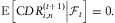
Because our successive Bayesian predictions (4.2) are (Ft)t-martingales we obtain the identity
 $${\Bbb E}\left[ {\left. {{\rm{C}}DR_{{i,n}}^{{(t\: + \,1)}} } \right|{{\scr F}_t}} \right]\: = \:0.$$
This explains that  $$)(-->$<> {\rm{C}}DR_{{i,n}}^{{(t\: + \:1)}} <$>
<!--$$ is typically predicted by 0 at time t, see also Merz & Wüthrich (Reference Merz and Wüthrich2008b). For the conditional MSEP of this prediction we obtain the identity
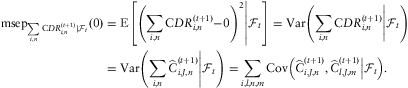 $${ {\rm{mse}}{{{\rm{p}}}_{\mathop{\sum}\limits_{i,n} {\rm{C}}DR_{{i,n}}^{{(t\: + \:1)}} |{{\scr F}_t}}}\left( 0 \right)\: = &\ \:{\Bbb E}\left[ {\left. {{{{\left( {\mathop{\sum}\limits_{i,n} {\rm{C}}DR_{{i,n}}^{{(t\: + \:1)}} {\rm{ - }}0} \right)}}^2} } \right|{{\scr F}_t}} \right]\: = \:{\rm{Var}}\left( {\left. {\mathop{\sum}\limits_{i,n} {\rm{C}}DR_{{i,n}}^{{(t\: + \:1)}} } \right|{{\scr F}_t}} \right) \cr = &\ \:{\rm{Var}}\left( {\left. {\mathop{\sum}\limits_{i,n} {\mathop{\widehat C}\nolimits^{}} _{{i,J,n}}^{{(t\: + \:1)}} } \right|{{\scr F}_t}} \right) \: = \: \mathop{\sum}\limits_{i,l,n,m} {\rm{Cov}}\left( {\left. {{\mathop{\widehat C}\nolimits^{}} _{{i,J,n}}^{{(t\: + \:1)}}, {\mathop{\widehat C}\nolimits^{}} _{{l,J,m}}^{{(t\: + \:1)}} } \right|{{\scr F}_t}} \right). \cr}$$
Our aim is to analyze the covariances on the right-hand side of this identity. Therefore, we need to rewrite the Bayesian ultimate claim predictors (4.2). Theorem 4.1 implies in a first step
 $${ {\mathop{\widehat C}\nolimits^{}} _{{i,J,n}}^{{(t + 1)}} = &\ {{C}_{i,t\: + \:1{\rm{ - }}i,n}}\,{\rm{exp}}\left\{ {\left( {{\bf {{e}}}{{^{\prime}}_{t\: + \:1|i,n}}\bimu _{{{\scr D}_{{t\: + \:1}}^{c} }}^{{{\rm{post}}}} \: + \:\frac{1}{2} {\bf {{e}}}{{^{\prime}}_{t\: + \:1|i,n}}S_{{{\scr D}_{{t\: + \:1}}^{c} }}^{{{\rm{post}}}} {{{\bf {{e}}}}_{t\: + \:1|i,n}}} \right){{1}_{\{ i\: + \:J \gt t\: + \:1\} }}} \right\} \cr = &\ {{C}_{i,t{\rm{ - }}i,n}}\,{\rm{exp}}\left\{ {{{\bixi }_{i,t\: + \:1{\rm{ - }}i,n}}\: + \:\left( {{{{\bf {{e}}}}^{\prime}_{t\: + \:1|i,n}}\bimu _{{{\scr D}_{{t\: + \:1}}^{c} }}^{{{\rm{post}}}} \: + \:\frac{1}{2} {{{\bf {{e}}}}^{\prime}_{t\: + \:1|i,n}}S_{{{\scr D}_{{t\: + \:1}}^{c} }}^{{{\rm{post}}}} {{{\bf {{e}}}}_{t\: + \:1|i,n}}} \right){{1}_{\{ i\: + \:J \gt t\: + \:1\} }}} \right\}, \cr}$$
where 1{·} denotes the indicator function. Observe that only the first two terms in the above exponent depend on the observations  $$)(-->$<> {{{\bf {{\bixi }}}}^{{{{\scr D}}_{t\, + \,1}}}} <$>
<!--$$ at time t + 1, and this dependence is linearly as we will just show. In analogy to (3.1) we decouple (bijectively) these observations in Dt +1 as follows:
 $${{\bixi }^{{{\scr D}_{t\: + \:1}}}} \mapsto ({{\bixi }^{{{\scr D}_t}}}, {{\bixi }^{{{\scr D}_{t\: + \:1}}\backslash {{\scr D}_t}}} ).$$
The first term describes the components that are observable at time t and the second term the components that are observed in accounting year t + 1, which also means  $$)(-->$<> {{{\scr D}}_{t\: + \:1}}\:\backslash \:{{{\scr D}}_t}\: \subset \:{\scr D}_{t}^{c} <$>
<!--$$. Thus, for the latter components we also need to apply Theorem 3.4, conditionally given Ft.
The first random term on the right-hand side of (5.2), given Ft, is  $$)(-->$<>\bixi<$>
<!--$$i ,t + 1−i ,n. We define a linear map by choosing
 $$)(-->$<> {{{\bf {{b}}}}_{t|i,n}}\: \in \:{{{\Bbb R}}^{|{\scr D}_{t}^{c} |}} <$>
<!--$$ such that
 $$)(-->$<> {\bf {{b}}}{{^{\prime}}_{t|i,n}} {{\bixi }^{{\scr D}_{t}^{c} }} \: = \:{{\bixi }_{i,t\: + \:1{\rm{ - }}i,n}} <$>
<!--$$. The second random term on the right-hand side of (5.2) is given by
 $$ \bimu _{{{\scr D}_{{t\: + \:1}}^{c} }}^{{{\rm{post}}}} \: = \:{{\bimu }_{{\scr D}_{{t\: + \:1}}^{c} }}\: + \:{{S}_{{\scr D}_{{t\: + \:1}}^{c}, {{\scr D}_{t\: + \:1}}}} {{\left( {{{S}_{{{\scr D}_{t\: + \:1}}}}} \right)}^{{\rm{ - }}1}} \left( {{{{\bf {{\bixi }}}}^{{{\scr D}_{t\: + \:1}}}} {\rm{ - }}{{\bimu }_{{{\scr D}_{t\: + \:1}}}}} \right). $$
We decouple  $$)(-->$<> {{\bixi }^{{{{\scr D}}_{t\, + \,1}}}} <$>
<!--$$. We define the linear function
 $$)(-->$<> {{B}_{t\: + \:1}}:{{{\Bbb R}}^{|{{{\scr D}}_{t\: + \:1}}|}} \: \rightarrow \:{{{\Bbb R}}^{|{{{\scr D}}_{t\: + \:1}}|}} <$>
<!--$$ with
 $${{B}_{t\: + \:1}}{{\bixi }^{{{\scr D}_{t\: + \:1}}}} \: = \:{{\left( {{{\xi }_{i,j,n}}{{{ 1}}_{\{ i\: + \:j\: = \:t\: + \:1\} }}} \right)}^{\prime}_{(i,j,n) \in {{\scr D}_{t\: + \:1}}}},$$
that is, all components of  $$)(-->$<> {{\bixi }^{{{{\scr D}}_{t\: + \:1}}}} <$>
<!--$$ are set equal to 0 if they are Ft-measurable. This implies
 $$ {{\bixi }^{{{\scr D}_{t\: + \:1}}}} \: = \:\left( {{\Bbb1}{\rm{ - }}{{B}_{t\: + \:1}}} \right){{\bixi }^{{{\scr D}_{t\: + \:1}}}} \: + \:{{B}_{t\: + \:1}}{{\bixi }^{{{\scr D}_{t\: + \:1}}}}, $$
where the first term is Ft-measurable and the second term exactly corresponds to observations in accounting year t + 1, i.e. to components in  $$)(-->$<> {{\scr D}_{t\: + \:1}}\:\backslash \:{{\scr D}_t}\: \subset \:{\scr D}_{t}^{c} <$>
<!--$$.
To simplify notation we define a linear map by choosing  $$)(-->$<> {{{\bf {{p}}}}_{t|i,n}} \in {{{\Bbb R}}^{|{\scr D}_{t}^{c} |}} <$>
<!--$$ such that
 $${\bf {{p}}}{{^{\prime}}_{t|i,n}}{{{\bf {{\bixi }}}}^{{\scr D}_{t}^{c} }} \: = \:{\bf {{b}}}{{^{\prime}}_{t|i,n}}{{{\bf {{\bixi }}}}^{{\scr D}_{t}^{c} }} \: + \:{{1}_{\{ i\: + \:J\, \gt \,t\: + \:1\} }} {\bf {{e}}}{{^{\prime}}_{t\: + \:1|i,n}}{{S}_{{\scr D}_{{t\: + \:1}}^{c}, {{{\scr D}}_{t\: + \:1}}}} {{\left( {{{S}_{{{{\scr D}}_{t\: + \:1}}}}} \right)}^{{\rm{ - }}1}} {{B}_{t\: + \:1}}{{{\bf {{\bixi }}}}^{{{{\scr D}}_{t\: + \:1}}}} .$$
This then allows to rewrite (5.2) as follows
 $${\mathop{\widehat C}\nolimits^{}} _{{i,J,n}}^{{(t + 1)}} \: = \:{{g}_{t|i,n}}({{\scr F}_t})\,{\rm{exp}}\left\{ {{\bf {{p}}}{{^{\prime}}_{t|i,n}}{{\bixi }^{{\scr D}_{t}^{c} }} } \right\},$$
for an appropriate Ft-measurable (constant)  $$)(-->$<> {{g}_{t|i,n}}({{\scr F}_t}) <$>
<!--$$.
Lemma 5.1 Under Model Assumptions 2.1 we have
 $${{g}_{t|i,n}}({{\scr F}_t})\: = \:{{C}_{i,t{\rm{ - }}t,n}}\,{\rm{exp}}\left\{ {({\bf {{e}}}{{^{\prime}}_{t|i,n}}{\rm{ - }}{\bf {{p}}}{{^{\prime}}_{t|i,n}})\bimu _{{{\scr D}_{t}^{c} }}^{{{\rm{post}}}} \: + \:\frac{1}{2}{\bf {{e}}}{{^{\prime}}_{t|i,n}}S_{{{\scr D}_{t}^{c} }}^{{{\rm{post}}}} {{{\bf {{e}}}}_{t|i,n}}{\rm{ - }}\frac{1}{2}{\bf {{p}}}{{^{\prime}}_{t|i,n}}S_{{{\scr D}_{t}^{c} }}^{{{\rm{post}}}} {{{\bf {{p}}}}_{t|i,n}}} \right\}.$$
We are now ready to state the main theorem for the conditional MSEP of the CDR. Its single terms in (5.1) are given by the following result.
Theorem 5.2 (CDR prediction uncertainty)Under Model Assumptions 2.1 we have for t∈{I,…,I + J−1}, i,l∈{t−J + 1,…,I} and n,m∈{1,…,N}
 $$ {\rm{Cov}}\left( {\left. {{\mathop{\widehat C}\nolimits^{}} _{{i,J,n}}^{{(t\, + \,1)}}, {\mathop{\widehat C}\nolimits^{}} _{{l,J,m}}^{{(t\, + \,1)}} } \right|{{\scr F}_t}} \right)\: = \:{\mathop{\widehat C}\nolimits^{}} _{{i,J,n}}^{{(t)}} {\mathop{\widehat C}\nolimits^{}} _{{l,J,m}}^{{(t)}} \left( {{\rm{exp}}\left\{ {{\bf {{p}}}{{^{\prime}}_{t|i,n}} S_{{{\scr D}_{t}^{c} }}^{{{\rm{post}}}} {{{\bf {{p}}}}_{t|l,m}}} \right\}{\rm{ - }}1} \right). $$
Before we are going to describe examples we need to slightly modify the vectors  $$)(-->$<> {{{\bf {{p}}}}_{t|i,n}} <$>
<!--$$ in order to get handy formulas in the implementation.
Lemma 5.3 Under the above assumptions we have
 $${{B}_{t\: + \:1}}{{\bixi }^{{{\scr D}_{t\: + \:1}}}} \: = \:({{P}_{{{\scr D}_{t\: + \:1}}}}{{P^{\prime}}_{{\scr D}_{t}^{c} }})\,{{\bixi }^{{\scr D}_{t}^{c} }} \; \; {{and}}\; \; {\bf {{b}}}{{^{\prime}}_{t|i,n}} {{\bixi }^{{\scr D}_{t}^{c} }} \: = \:{\bf {{e}}}{{^{\prime}}_{t|i,n}}\,({{P}_{{\scr D}_{t}^{c} }}{{P^{\prime}}_{{{\scr D}_{t\, + \,1}}}}{{P}_{{{\scr D}_{t\, + \,1}}}}{{P^{\prime}}_{{\scr D}_{t}^{c} }})\,{{\bixi }^{D_{t}^{c} }} .$$
This lemma has the nice consequence that we can express  $$)(-->$<> {\bf {{p}}}{{^{\prime}}_{t|i,n}} <$>
<!--$$ in terms that have already been introduced in Section 4, namely
 $${\bf {{p}}}{{^{\prime}}_{t|i,n}}\: = \:\left( {{\bf {{e}}}{{^{\prime}}_{t|i,n}} ({{P}_{{\scr D}_{t}^{c} }}{{{P^{\prime}}}_{{{\scr D}_{t\: + \:1}}}})\: + \:{{1}_{\{ i\: + \:J \gt t\: + \:1\} }} {\bf {{e}}}{{^{\prime}}_{t\: + \:1|i,n}}{{S}_{{\scr D}_{{t\: + \:1}}^{c}, {{\scr D}_{t\: + \:1}}}} {{{\left( {{{S}_{{{\scr D}_{t\: + \:1}}}}} \right)}}^{{\rm{ - }}1}} } \right)({{P}_{{{\scr D}_{t\: + \:1}}}}{{P^{\prime}}_{{\scr D}_{t}^{c} }}).$$
6 Examples and sensitivities
In this section we study the influence of different choices of the covariance structure  $$)(-->$<> \rSigma \, \in \,{{{\Bbb R}}^{d\,\times \,d}} <$>
<!--$$ on the resulting claims reserves
 $$)(-->$<> {\mathop{\widehat R}\nolimits^{}} _{{i,n}}^{{(t)}} <$>
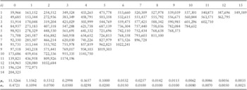
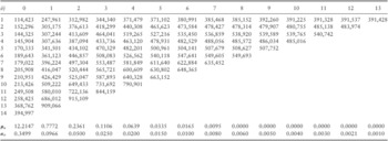
<!--$$ (Theorem 4.1) and the corresponding conditional MSEP's for the ultimate claim prediction (Theorem 4.3) and for the CDR prediction (Theorem 5.2). Therefore, we revisit the multivariate data studied in Braun (Reference Braun2004). It consists of N = 2 claims reserving triangles. The first triangle (n = 1) describes a general liability (GL) insurance run-off (see Table 5 in the Appendix), the second triangle (n = 2) describes a motor third party liability (MTPL) insurance run-off (see Table 6 in the Appendix).
We make different choices for the covariance matrix  $$)(-->$<>\rSigma<$>
<!--$$. First we rewrite this covariance matrix
 $$)(-->$<>\rSigma<$>
<!--$$ in order to get a better understanding. Similar to the prior mean μ we assume that the conditional standard deviation of
 $$)(-->$<>\xi<$>
<!--$$i,j,n does not depend on the accident year i∈{1,…,I}, thus
 $${\rm{Var}}{{\left( {\left. {{{\xi }_{i,j,n}}} \right|{\bf {{\brTheta }}}} \right)}^{1/2}} \: = \:{{\sigma }_{j,n}}\; \; {\rm{for}}\,{\rm{all}}\,(i,j,n)\: \in \:{\scr J}.$$
We define the standard deviation vectors  $$)(-->$<> {{{\bf {{\bisigma }}}}_ \bullet }\: = \:({{\sigma }_{0,1}}, \ldots, {{\sigma }_{0,N}}, \ldots, {{\sigma }_{J,1}}, \ldots, {{\sigma }_{J,N}})^{\prime}\, \in \,{{{\Bbb R}}^a} <$>
<!--$$ for
 $$)(-->$<>\bixi<$>
<!--$$i and
 $$)(-->$<> {\bf {{\bisigma }}}\, = \,A{{{\bf {{\bisigma }}}}_ \bullet }\, \in \,{{{\Bbb R}}^d} <$>
<!--$$ for
 $$)(-->$<>\bixi<$>
<!--$$. With this notation at hand we can rewrite the covariance matrix
 $$)(-->$<>\rSigma<$>
<!--$$ as
 $${\rm{Cov}}\left( {\left. \bixi \right|{\bf {{\brTheta }}}} \right) \: = \:\rSigma \: = \:{\rm{diag}}({\bf {{\bisigma }}})\,\rLambda \,{\rm{diag}}({\bf {{\bisigma }}}),$$
where  $$)(-->$<> \rLambda \, \in \,{{{\Bbb R}}^{d\,\times \,d}} <$>
<!--$$ denotes the conditional correlation matrix of
 $$)(-->$<>\bixi<$>
<!--$$. The numerical values of the chosen standard deviation parameter
 $$)(-->$<>\sigma<$>
<!--$$ are given in Tables 5 and 6 below. Our aim in the next sections is to examine different (positive-definite) choices of the correlation matrix Λ. For the prior uncertainty in Θ we choose T = τ 21 with τ = 1 (this is a rather non-informative choice and the diagonal structure of T implies that prior uncertainty on the two portfolios is mutually independent).
6.1 Uncorrelated choice for Λ
As a benchmark model we consider Λ =  $$)(-->$<>\Bbb {1}<$>
<!--$$, i.e. all components of
 $$)(-->$<>\bixi<$>
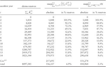
<!--$$ are conditionally independent, given Θ. This is a Bayesian version of Hertig's log-normal claims reserving model, see Hertig (Reference Hertig1985). It corresponds to the model typically analyzed in practice where one assumes that payments in different accident years i are independent, conditionally given the model parameters (see also Mack (Reference Mack1993)). Under these model assumptions we obtain the results provided in Table 1. In this table we give the claims reserves and the corresponding conditional MSEP's, based on the information
 $$)(-->$<> {\cal F}_{I}<$>
<!--$$, for single accident years i∈{1,…,14} and on the line ‘‘total” for aggregated accident years
 $$)(-->$<> \mathop{\sum}\nolimits_{i\: = \:1}^{14} <$>
<!--$$. We observe that the calculated total claims reserves
 $$)(-->$<> \mathop{\sum}\nolimits_{i,n} {\mathop{R}\nolimits^{}} _{{i,n}}^{{(I)}} <$>
<!--$$ (aggregated over all accident years i∈{1,…,14} and all sub-portfolios n∈{1,2}) result in the value 8097,585.
Uncorrelated case Λ =  $$)(-->$<>\Bbb {1}<$>
<!--$$ for the aggregated GL and MTPL portfolio
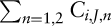 $$)(-->$<> \mathop{\sum}\sidelimits_{n\: = \:1,2} {{C}_{i,J,n}} <$>
<!--$$.

Our first aim is to study the conditional MSEP's in this benchmark model. We have, in view of formula (4.4),
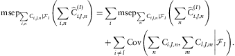 $$ { {\rm{mse}}{{{\rm{p}}}_{\mathop{\sum}\limits_{i,n} {{C}_{i,J,n}}|{{\scr F}_I}}}\left( {\mathop{\sum}\limits_{i,n} {\mathop{\widehat C}\nolimits^{}} _{{i,J,n}}^{{(I)}} } \right) = & \mathop{\sum}\limits_i {\rm{mse}}{{{\rm{p}}}_{\mathop{\sum}\limits_n {{C}_{i,J,n}}|{{\scr F}_I}}}\left( {\mathop{\sum}\limits_n {\mathop{\widehat C}\nolimits^{}} _{{i,J,n}}^{{(I)}} } \right) \cr & + \mathop{\sum}\limits_{i\, \ne \,l} {\rm{Cov}}\left( {\left. {\mathop{\sum}\limits_n {{C}_{i,J,n}},\mathop{\sum}\limits_m {{C}_{l,J,m}}} \right|{{\scr F}_I}} \right). \cr} $$
The first term on the right-hand side (rhs) of (6.1) is the conditional MSEP for single accident years (which is given on lines i = 1,…,14 in Table 1). The second term on the rhs of (6.1) corresponds to the implied covariance from the simultaneous parameter uncertainty in Θ over all accident years, that is,
 $$ { \mathop{\sum}\limits_{i\, \ne \,l} {\rm{Cov}}\left( {\left. {\mathop{\sum}\limits_n {{C}_{i,J,n}},\mathop{\sum}\limits_m {{C}_{l,J,m}}} \right|{{\scr F}_I}} \right) \, = \, & \mathop{\sum}\limits_{i\, \ne \,l} {\Bbb E}\left[ {\left. {{\rm{Cov}}\left( {\left. {\mathop{\sum}\limits_n {{C}_{i,J,n}},\mathop{\sum}\limits_m {{C}_{l,J,m}}} \right|{{\scr F}_I},{\bf {{\brTheta }}}} \right)} \right|{{\scr {F}}_I}} \right] \cr \, &+ \,\mathop{\sum}\limits_{i\, \ne \,l} {\rm{Cov}}\left( {\left. {\mathop{\sum}\limits_n {\Bbb E}\left[ {\left. {{{C}_{i,J,n}}} \right|{{\scr F}_I},{\bf {{\brTheta }}}} \right],\mathop{\sum}\limits_m {\Bbb E}\left[ {\left. {{{C}_{l,J,m}}} \right|{{\scr F}_I},{\bf {{\brTheta }}}} \right]} \right|{{\scr F}_I}} \right). \cr} $$
The first term on the rhs is equal to zero (due to the uncorrelated choice given by Λ =  $$)(-->$<>\Bbb {1}<$>
<!--$$). The square-root of the second term is given by 217,693 (and for the CDR uncertainty by 151,274, see Table 1). This allows to define the implied average correlation between accident years
 $$)(-->$<> {{\bar{\psi }}_{{\rm{a}}.{\rm{y}}.}}(0) <$>
<!--$$ by
 $$ {{\bar{\psi }}_{{\rm{a}}.{\rm{y}}.}}(0) {\mathop{ = }\limits^{{{\rm{def}}.}}} \, \frac{{\mathop{\sum}\nolimits_{i\, \ne \,l} {\rm{Cov}}\left( {\left. {\mathop{\sum}\nolimits_n {{C}_{i,J,n}},\mathop{\sum}\nolimits_m {{C}_{l,J,m}}} \right|{{\scr F}_I}} \right)}}{{\mathop{\sum}\nolimits_{i\, \ne \,l} {\rm{Var}}{{{\left( {\left. {\mathop{\sum}\nolimits_n {{C}_{i,J,n}}} \right|{{\scr F}_I}} \right)}}^{1/2}} {\rm{Var}}{{{\left( {\left. {\mathop{\sum}\nolimits_m {{C}_{l,J,m}}} \right|{{\scr F}_I}} \right)}}^{1/2}} }}\, = \,5.2\% . $$
Thus, the implied average correlation between accident years of the joint parameter uncertainty in Θ is 5.2% in our example. Completely analogously we obtain for the implied average correlation between accident years for the CDR uncertainty  $$)(-->$<> \bar{\psi }_{{{\rm{a}}.{\rm{y}}.}}^{{{\rm{CDR}}}} (0)\, = \,4.9\% <$>
<!--$$. These implied correlations play an important role in practice because typically they are specified/adjusted by experts. However, we will see that this notion can be quite controversial and even misleading.
6.2 Accounting year correlation and portfolio independence for Λ
In the spirit of Wüthrich (Reference Wüthrich2010) we introduce accounting year dependence, but for the time-being we assume that the different portfolios n∈{1,…, N} are still independent. Thus, the correlation matrix Λ is chosen such that for a fixed ρ∈[0,1) we have
 $$ {\rm{Cov}}\left( {\left. {{{\xi }_{i,j,n}},{{\xi }_{l,k,n}}} \right|{\bf {{\brTheta }}}} \right)\, = \,{{\sigma }_{j,n}} {{\sigma }_{k,n}} \rho {{ 1}_{\{ i\, + \,j\, = \,l\, + \,k\} }}\; \; {\rm{for}}\,(i,j)\, \ne \,(l,k), $$
 $$ {\rm{Cov}}\left( {\left. {{{\xi }_{i,j,n}},{{\xi }_{l,k,m}}} \right|{\bf {{\brTheta }}}} \right)\, = \,0\; \; \; \; {\rm{for}}\;n\, \ne \,m. $$
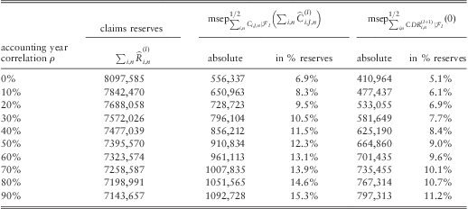
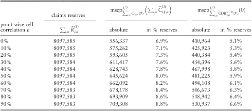
The results for these choices (6.3)–(6.4) are given in Table 2. The first observation is that the claims reserves are a decreasing function in ρ. Though very important, this observation should not be over-stated because depending on the numerical example we may also obtain an increasing function in ρ for the claims reserves. This decrease of the claims reserves is related to the fact that the data does not satisfy assumption (2.3) and we should adjust for this using prior differences as described in Remarks 2.2. To fully understand this adjustment more analysis on the micro-level of the data needs to be done. We refrain from doing so here because we would like to concentrate on the uncertainties given by the conditional MSEP's.
Accounting year correlation ρ and portfolio independence according to (6.3)–(6.4).
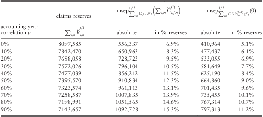
A very important observation is that the conditional MSEP's are an increasing function in ρ. For example, a correlation parameter of ρ = 20% leads to a substantial increase of the square-rooted CDR uncertainty of
 $$\frac{{533,055}}{{410,964}}{\rm{ - }}1\, \approx \,30\% !$$
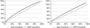
The full curve is given in Figure 1(a) (lhs) where we see that this increase is a non-linear function that needs to be analyzed in a careful bottom-up approach.
Accounting year correlation ρ and portfolio independence according to (6.3)–(6.4): (a) lhs: relative increase of square-rooted uncertainties as a function of the accounting year correlation ρ∈[0,1) for  $$)(-->$<> {\rm{msep}}_{{\mathop{\sum}\sidelimits_{i,n} {{C}_{i,J,n}}|{{\cal F}_I}}}^{{1/2}} \left( {\mathop{\sum}\sidelimits_{i,n} {\mathop{\widehat C}\nolimits^{}} _{{i,J,n}}^{{(I)}} } \right) <$>
<!--$$ and
 $$)(-->$<> {\rm{msep}}_{{\mathop{\sum}\sidelimits_{i,n} {\rm{C}}DR_{{i,n}}^{{(I\, + \,1)}} |{{\scr F}_I}}}^{{1/2}} \left( 0 \right) <$>
<!--$$; (b) rhs: average implied correlations between accident years
 $$)(-->$<> {{\bar{\psi }}_{{\rm{a}}.{\rm{y}}.}}(\rho ) <$>
<!--$$ and
 $$)(-->$<> \bar{\psi }_{{{\rm{a}}.{\rm{y}}.}}^{{{\rm{CDR}}}} (\rho ) <$>
<!--$$ as a function of the accounting year correlation ρ∈[0,1).

Conclusion 1The introduction of accounting year dependence may substantially increase the prediction uncertainty. This relative increase is non-linear in the correlation parameter ρ∈[0,1) (Figure 1(a), lhs).
Next we calculate the average implied correlations between accident years  $$)(-->$<> {{\bar{\psi }}_{{\rm{a}}.{\rm{y}}.}}(\rho ) <$>
<!--$$ and
 $$)(-->$<> \bar{\psi }_{{{\rm{a}}.{\rm{y}}.}}^{{{\rm{CDR}}}} (\rho ) <$>
<!--$$ as a function of the accounting year correlation ρ∈[0,1) (see also (6.2)). We define these average implied correlations between accident years by
 $$ {{\bar{\psi }}_{{\rm{a}}.{\rm{y}}.}}(\rho )\, {\mathop{ = }\limits^{{{\rm{def}}.}}} \, \frac{{\mathop{\sum}\sidelimits_{i\, \ne \,l} {\rm{Co}}{{{\rm{v}}}^{(\rho )}} \left( {\left. {\mathop{\sum}\sidelimits_n {{C}_{i,J,n}},\mathop{\sum}\sidelimits_m {{C}_{l,J,m}}} \right|{{\cal F}_I}} \right)}}{{\mathop{\sum}\nolimits_{i\, \ne \,l} {\rm{Va}}{{{\rm{r}}}^{(0)}} {{{\left( {\left. {\mathop{\sum}\nolimits_n {{C}_{i,J,n}}} \right|{{\cal F}_I}} \right)}}^{1/2}} {\rm{Va}}{{{\rm{r}}}^{(0)}} {{{\left( {\left. {\mathop{\sum}\sidelimits_m {{C}_{l,J,m}}} \right|{{\cal F}_I}} \right)}}^{1/2}} }}, $$
where Cov(ρ)(·,·∣FI) corresponds to the choice ρ∈[0,1) and Var(0)(·∣FI) to the choice ρ = 0. The results are presented in Figure 1(b) (rhs). We see that  $$)(-->$<> {{\bar{\psi }}_{{\rm{a}}.{\rm{y}}.}}(\rho ) <$>
<!--$$ and
 $$)(-->$<> \bar{\psi }_{{{\rm{a}}.{\rm{y}}.}}^{{{\rm{CDR}}}} (\rho ) <$>
<!--$$ are non-linearly increasing functions in ρ. More surprisingly, we see that
 $$)(-->$<> {{\bar{\psi }}_{{\rm{a}}.{\rm{y}}.}}(\rho )\, \gt \,1 <$>
<!--$$ for ρ > 85% which seems to be an error at first sight. However, these figures are correct and there results a counter-intuitive correlation bigger than 1! The reason for this value bigger than 1 is that (6.5) does not give a well-specified correlation measure because enumerator and denominator belong to different models (specifications of ρ). For different ρ's also the conditional MSEP's for single accident years i (given in Table 1 for ρ = 0) will change; and thus Table 1 does not allow to reconstruct the results for ρ > 0 using an average implied correlation factor (bounded by 1). We conclude again that only a bottom-up calculation can provide the full flavour of the results, because if we need to reconstruct Table 1 for ρ > 0 then we directly obtain the full picture of the overall uncertainties.
Conclusion 2The introduction of an average implied correlation between accident years given by (6.5) does not allow to construct the conditional MSEP's for ρ > 0 from the conditional MSEP's with ρ = 0 in an intuitive way, because  $$)(-->$<> {{\bar{\psi }}_{{\rm{a}}.{\rm{y}}.}}(\rho ) <$>
<!--$$can take arbitrary and counter-intuitive values (Figure 1(b), rhs).
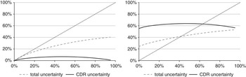
The next observation on the average implied correlation between accident years came as a surprise to us (and at first glance it seemed very counter-intuitive). To see this next phenomenon we need to choose a different data set. We choose the MTPL data from Saluz et al. (Reference Saluz, Gisler and Wüthrich2011), Table 7 (and we set N = 1). Figure 2 shows that the square-rooted conditional MSEP  $$)(-->$<> {\rm{msep}}_{{\mathop{\sum}\sidelimits_i {{C}_{i,J,1}}|{{\scr F}_I}}}^{{1/2}} \left( {\mathop{\sum}\sidelimits_i {\mathop{\widehat C}\nolimits^{}} _{{i,J,1}}^{{(I)}} } \right) <$>
<!--$$ of the total ultimate claim prediction and the corresponding implied average correlation
 $$)(-->$<> {{\bar{\psi }}_{{\rm{a}}{\rm{.y}}.}}(\rho ) <$>
<!--$$ are increasing functions in the accounting year correlation ρ. The picture for the CDR is very different: in this example the conditional MSEP
 $$)(-->$<> {\rm{mse}}{{{\rm{p}}}_{\mathop{\sum}\sidelimits_i {\rm{C}}DR_{{i,1}}^{{(I\, + \,1)}} |{{\scr F}_I}}}\left( 0 \right) <$>
<!--$$ is not an increasing function of the accounting year correlation parameter ρ! There are two arguments for this non-monotonicity property: (1) the ultimate claim predictor
 $$)(-->$<> {\mathop{\widehat C}\nolimits^{}} _{{i,J,1}}^{{(I)}} <$>
<!--$$ is in this example a decreasing function in ρ (similar to Table 2) and this decrease cannot be compensated by an increase of the covariance term
 $$)(-->$<> ({\rm{exp}}\{ {\bf {{p}}}{{^{\prime}}_{I|i,1}}\,S_{{{\scr D}_{I}^{c} }}^{{{\rm{post}}}} \,{{{\bf {{p}}}}_{I|l,1}}\} {\rm{ - }}1) <$>
<!--$$, see Theorem 5.2; (2) the CDR uncertainty measures possible changes over the next accounting year whereas the ultimate claim prediction uncertainty measures the total uncertainty until all claims are settled. An increasing accounting year correlation ρ may also imply that more parameter uncertainty is shifted from the next year to latter periods, and hence the one-year CDR uncertainty (for the next accounting year) is relatively decreasing compared to the total uncertainty.
Example Saluz et al. (Reference Saluz, Gisler and Wüthrich2011), Table 7: Accounting year correlation ρ according to (6.3): (a) lhs: relative increase of square-rooted uncertainties as a function of the accounting year correlation ρ∈[0,1) for  $$)(-->$<> {\rm{msep}}_{{\mathop{\sum}\sidelimits_i {{C}_{i,J,1}}|{{\scr F}_I}}}^{{1/2}} \left( {\mathop{\sum}\sidelimits_i {\mathop{\widehat C}\sidelimits^{}} _{{i,J,1}}^{{(I)}} } \right) <$>
<!--$$ and
 $$)(-->$<> {\rm{msep}}_{{\mathop{\sum}\sidelimits_i {\rm{C}}DR_{{i,1}}^{{(I\, + \,1)}} |{{\scr F}_I}}}^{{1/2}} \left( 0 \right) <$>
<!--$$; (b) rhs: average implied correlations between accident years
 $$)(-->$<> {{\bar{\psi }}_{{\rm{a}}.{\rm{y}}.}}(\rho ) <$>
<!--$$ and
 $$)(-->$<> \bar{\psi }_{{{\rm{a}}.{\rm{y}}.}}^{{{\rm{C}}DR}} (\rho ) <$>
<!--$$ as a function of the accounting year correlation ρ∈[0,1).

Conclusion 3The average implied correlation between accident years is not necessarily an increasing function in the accounting year correlation parameter ρ (Figure 2(b), rhs).
6.3 Accounting year independence and portfolio correlation for Λ
In this section we study portfolio correlation in the spirit of Braun (Reference Braun2004) and Merz & Wüthrich (Reference Merz and Wüthrich2007, Reference Merz and Wüthrich2008a), but we assume that there is no accounting year correlation. Thus, the correlation matrix Λ is chosen such that for a fixed ρ∈[0,1) we have
 $$ {\rm{Cov}}\left( {\left. {{{\xi }_{i,j,n}},{{\xi }_{l,k,m}}} \right|{\bf {{\brTheta }}}} \right)\, = \,{{\sigma }_{j,n}} {{\sigma }_{k,m}} \rho {{ 1}_{\{ (i,j)\, = \,(l,k)\} }}\; \; {\rm{for}}\;(i,j,n)\, \ne \,(l,k,m), $$
i.e. this is a point-wise cell dependence between  $$)(-->$<>\bixi<$>
<!--$$i,j,n and
 $$)(-->$<>\bixi<$>
<!--$$i,j,m. The results for these choices (6.6) are given in Table 3. We observe that the increase in prediction uncertainty is comparably small under assumption (6.6) (compare Tables 2 and 3). Under assumption (6.6) the relative increase in the square-rooted conditional MSEP can be at most
 $$)(-->$<>\sqrt 2 {\rm{ - 1}}\,{\rm{ = }}\,{\rm{41}}{\rm{.4\% }} <$>
<!--$$, whereas under assumptions (6.3)–(6.6) we can get relative increases of 100% (see Figure 1(a), lhs). Thus, if we only apply this type of point-wise cell correlation, then prediction uncertainty is typically under-estimated because data show more dependence structure.
Point-wise cell correlation ρ and accounting year independence according to (6.6).
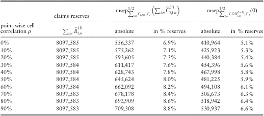
Conclusion 4Point-wise cell dependence only allows for a moderate increase in the uncertainty estimates.
Conclusions 1 and 4 are in line with the findings in Shi et al. (Reference Shi, Basu and Meyers2012), Table 2.
6.4 Accounting year and portfolio correlation for Λ
Finally, we combine the two previous forms of dependence. We choose  $$)(-->$<>\rSigma<$>
<!--$$ such that for ρ∈[0,1)
 $$ {\rm{Cov}}\left( {\left. {{{\xi }_{i,j,n}},{{\xi }_{l,k,m}}} \right|{\bf {{\brTheta }}}} \right)\, = \,{{\sigma }_{j,n}} {{\sigma }_{k,m}}\,\rho {{ 1}_{\{ i + j = l + k\} }}\; \; {\rm{for}}\;(i,j,n)\, \ne \,(l,k,m). $$
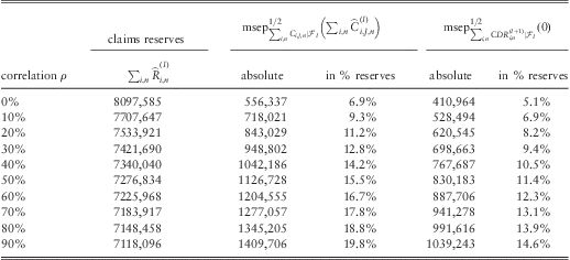
The results for these choices (6.7) are given in Table 4. We see a substantial increase in the uncertainty if we combine these two different types of dependence. E.g., if we choose ρ = 20% we obtain the following relative increases in the CDR uncertainty:
Accounting year and portfolio correlation according to (6.7).
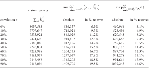

That is, already a “comparably moderate” correlation parameter of ρ = 20% implies in model (6.7) an increase of CDR uncertainty of 51% (measured in the square-rooted conditional MSEP). If we start from the uncorrelated model ρ = 0 we obtain portfolio uncertainties
 $$ {\rm{msep}}_{{\mathop{\sum}\limits_i {\rm{C}}DR_{{i,n}}^{{(I\, + \,1)}} |{{\scr F}_I}}}^{{1/2}} \left( 0 \right)\, = \,\left\{ {\matrix{ {372,690} & {{\rm{for}}\;n\, = \,1,} \cr\ {172,613} & {{\rm{for}}\;n\, = \,2.} \\\end{}} \right $$
A “correlation” factor of 1 between these two latter figures implies a total uncertainty of 372,690 + 172,613 = 545,569 which is by far less than the 620,545 from model (6.7) with ρ = 20%. Thus, we get the following conclusion.
Conclusion 5An overall top correlation as specified in Solvency 2 (see European Commission (2010), SCR.9.34) or in the Swiss Solvency Test (see Swiss Solvency Test (2006), Section 8.4) typically under-estimates the prediction uncertainty if one starts with the benchmark model ρ = 0.
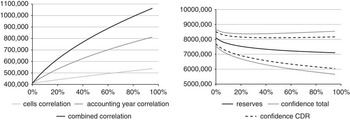
Finally, in Figure 3(a) (lhs) we compare the square-rooted conditional MSEPs for the CDR uncertainties as a function of ρ for the three models considered above. We observe the non-linear increase which can only be calculated in a bottom-up approach (as suggested above). Figure 3(b) (rhs) gives the claims reserves from Corollary 4.2 together with a confidence interval of 1-standard deviation, both for the total uncertainty (Theorem 4.3) and the CDR uncertainty (Theorem 5.2) as a function of the correlation parameter ρ.
(a) lhs: comparison of models (6.3)–(6.4) (accounting year correlation), (6.6) (point-wise cells correlation) and (6.7) (combined correlation), we display the square-rooted conditional MSEPs of the CDR uncertainty as a function of ρ∈[0,1); (b) rhs: combined correlation model (6.7), claims reserves and 1-standard deviation confidence interval for the total uncertainty and the CDR uncertainty as a function of ρ∈[0,1).

7 Conclusions
We summarize the findings and give a brief outlook:
• There is no reasonable way (short-cut) to choose correlation on a top level because often intuition fails as Conclusions 1–5 show. Overall correlations can only be determined in a bottom-up approach.
• We provide the whole tool kit (Theorems 4.3 and 5.2) for this bottom-up approach in the multivariate log-normal model. Other distributional models can often only be solved numerically and then the sensitivity analysis becomes much intransparent.
• Other risk measures than the conditional MSEP (such as Value-at-Risk or Tail-Value-at-Risk) can only be calculated numerically. In addition, it would be interesting to analyze the behaviour of these risk measures under dependence structures with tail dependence, see McNeil et al. (Reference McNeil, Frey and Embrechts2005).
• The choice of the (positive-definite) covariance matrix
$$)(-->$<>\rSigma<$>
<!--$$ needs a thorough discussion. Sometimes data is helpful but we believe that expert opinion is as important as data in order to get reasonable choices for $$)(-->$<>\rSigma<$>
<!--$$. Often accounting year dependence is correlated with inflation that depends on financial market developments. Similar to König et al. (Reference König, Weber and Wüthrich2011) and Donnelly & Wüthrich (Reference Donnelly and Wüthrich2012) these dependence structures between insurance claims and financial market movements should be studied in order to enhance the quality of the prediction.• Sensitivities for different lines of business with different development patterns (and uncertainty) should be investigated in a comprehensive case study.


Appendix A Proofs of the statements
Proof of Theorem 3.1. We give three different proofs for Theorem 3.1 because all of them are interesting on their own.
Proof (1). The first proof goes by “brute force”. It uses classical Bayesian thinking that tries to determine the form of the posterior density explicitly. This proof is important because it shows how the model can be generalized to non-Gaussian model assumptions and how Markov chain Monte Carlo simulation methods need to be applied. We rewrite the joint density (2.2) of  $$)(-->$<>\bixi<$>
<!--$$ and Θ as follows (hiding all normalizing constants in the symbol
 $$)(-->$<>\propto<$>
<!--$$)
 $$ { {\rm{ - }}2{\rm{log}}f(\bixi, \bitheta ) & \propto \left( {\bixi {\rm{ - }}A\bitheta } \right)^{\prime}{{{\rm{\rSigma }}}^{{\rm{ - }}1}} \left( {\bixi {\rm{ - }}A\bitheta } \right)\, + \,\left( {\bitheta {\rm{ - }}\bimu } \right){^\prime}{{T}^{{\rm{ - }}1}} \left( {\bitheta {\rm{ - }}\bimu } \right) \cr &\propto \bixi ^{\prime}{{{\rm{\rSigma }}}^{{\rm{ - }}1}} \bixi {\rm{ - }}2\bitheta ^{\prime}A^{\prime}{{{\rm{\rSigma }}}^{{\rm{ - }}1}} \bixi \, + \,\bitheta ^{\prime}A^{\prime}{{{\rm{\rSigma }}}^{{\rm{ - }}1}} A\bitheta \, + \,\bitheta ^{\prime}{{T}^{{\rm{ - }}1}} \bitheta {\rm{ - }}2\bitheta ^{\prime}{{T}^{{\rm{ - }}1}} \bimu \cr & = \,\bixi ^{\prime}{{{\rm{\rSigma }}}^{{\rm{ - }}1}} \bixi {\rm{ - }}2\bitheta ^{\prime}\left( {A^{\prime}{{{\rm{\rSigma }}}^{{\rm{ - }}1}} \bixi \, + \,{{T}^{{\rm{ - }}1}} \bimu } \right)\, + \,\bitheta ^{\prime}\left( {A^{\prime}{{\rSigma }^{{\rm{ - }}1}} A\, + \,{{T}^{{\rm{ - }}1}} } \right)\bitheta . \cr} $$
We define the matrices  $$)(-->$<> {{B}^{{\rm{ - }}1}} \, = \,A^{\prime}{{{\rm{\rSigma }}}^{{\rm{ - }}1}} A\, + \,{{T}^{{\rm{ - }}1}} \, \in \,{{{\Bbb R}}^{a\times a}} <$>
<!--$$ and
 $$)(-->$<> C\, = \,A^{\prime}{{\rSigma }^{{\rm{ - }}1}} A\, \in \,{{{\Bbb R}}^{a\,\times \,a}} <$>
<!--$$. These matrices are positive-definite: choose
 $$)(-->$<> \bitheta \, \ne \,(0, \ldots, 0)^{\prime}\, \in \,{{{\Bbb R}}^a} <$>
<!--$$. The choice of A implies
 $$)(-->$<> A\bitheta \, \ne \,(0, \ldots, 0)^{\prime}\, \in \,{{{\Bbb R}}^d} <$>
<!--$$. Since
 $$)(-->$<>\rSigma<$>
<!--$$ is positive-definite we obtain for all these vectors θ
 $$\bitheta ^{\prime}C\bitheta \, = \,\bitheta ^{\prime}\left( {A^{\prime}{{\rSigma }^{{\rm{ - }}1}} A} \right)\bitheta \, = \,(A\bitheta )^{\prime}{{\rSigma }^{{\rm{ - }}1}} A\bitheta \, \gt \,0,$$
thus the matrix C is positive-definite. Moreover, T is positive-definite and hence B −1 = C + T −1 is positive-definite (and invertible).
We add and subtract the same term so that we obtain a density as a function of θ.
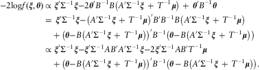 $${ {\rm{ - }}2{\rm{log}}f(\bixi, \bitheta ) & \propto \bixi ^{\prime}{{{\rm{\rSigma }}}^{{\rm{ - }}1}} \bixi {\rm{ - }}2\bitheta ^{\prime}{{B}^{{\rm{ - }}1}} B\left( {A^{\prime}{{{\rm{\rSigma }}}^{{\rm{ - }}1}} \bixi \, + \,{{T}^{{\rm{ - }}1}} \bimu } \right)\, + \,\bitheta ^{\prime}{{B}^{{\rm{ - }}1}} \bitheta \cr &= \,\bixi ^{\prime}{{{\rm{\rSigma }}}^{{\rm{ - }}1}} \bixi {\rm{ - }}\left( {A^{\prime}{{{\rm{\rSigma }}}^{{\rm{ - }}1}} \bixi \, + \,{{T}^{{\rm{ - }}1}} \bimu } \right)^{\prime}B^{\prime}{{B}^{{\rm{ - }}1}} B\left( {A^{\prime}{{\rSigma }^{{\rm{ - }}1}} \bixi \, + \,{{T}^{{\rm{ - }}1}} \bimu } \right) \cr & \quad + \left( {\bitheta {\rm{ - }}B\left( {A^{\prime}{{\rSigma }^{{\rm{ - }}1}} \bixi \, + \,{{T}^{{\rm{ - }}1}} \bimu } \right)} \right)^{\prime}{{B}^{{\rm{ - }}1}} \left( {\bitheta {\rm{ - }}B\left( {A^{\prime}{{\rSigma }^{{\rm{ - }}1}} \bixi \, + \,{{T}^{{\rm{ - }}1}} \bimu } \right)} \right) \cr & \propto \bixi ^{\prime}{{\rSigma }^{{\rm{ - }}1}} \bixi {\rm{ - }}\bixi ^{\prime}{{\rSigma }^{{\rm{ - }}1}} AB^{\prime}A^{\prime}{{\rSigma }^{{\rm{ - }}1}} \bixi {\rm{ - }}2\bixi ^{\prime}{{\rSigma }^{{\rm{ - }}1}} AB^{\prime}{{T}^{{\rm{ - }}1}} \bimu \cr & \quad+ \left( {\bitheta {\rm{ - }}B\left( {A^{\prime}{{\rSigma }^{{\rm{ - }}1}} \bixi \, + \,{{T}^{{\rm{ - }}1}} \bimu } \right)} \right)^{\prime}{{B}^{{\rm{ - }}1}} \left( {\bitheta \,{\rm{ - }}\,B\left( {A^{\prime}{{\rSigma }^{{\rm{ - }}1}} \bixi \, + \,{{T}^{{\rm{ - }}1}} \bimu } \right)} \right). \cr}$$
The last line provides a multivariate Gaussian density for θ. This implies, note that B′ = B,
 $$f(\bixi )\, = \,{\int}_{{{{\Bbb \!\!\!R}}^a} } f(\bixi, \bitheta ) d\bitheta \, \propto \,{\rm{exp}}\left\{ {{\rm{ - }}\frac{1}{2}\left( {\bixi ^{\prime}{{\rSigma }^{{\rm{ - }}1}} \bixi {\rm{ - }}\bixi ^{\prime}{{\rSigma }^{{\rm{ - }}1}} ABA^{\prime}{{\rSigma }^{{\rm{ - }}1}} \bixi {\rm{ - }}2\bixi ^{\prime}{{\rSigma }^{{\rm{ - }}1}} AB{{T}^{{\rm{ - }}1}} \bimu } \right)} \right\}.$$
Thus, we obtain a multivariate Gaussian distribution for  $$)(-->$<>\bixi<$>
<!--$$ and there remains to calculate its mean and variance. The unconditional mean of
 $$)(-->$<>\bixi<$>
<!--$$ is given by
 $${\Bbb E}\left[ \bixi \right]\, = \,{\Bbb E}\left[ {{\Bbb E}\left[ {\left. \bixi \right|{\bf {{\brTheta }}}} \right]} \right]\, = \,{\Bbb E}\left[ {A{\bf {{\brTheta }}}} \right]\, = \,A\bimu .$$
For the unconditional covariance matrix of  $$)(-->$<>\bixi<$>
<!--$$ we have
 $${\rm{Cov}}\left( \bixi \right)\: = \:{\Bbb E}\left[ {{\rm{Cov}}\left( {\left. \bixi \right|{\bf {{\brTheta }}}} \right)} \right]\: + \:{\rm{Cov}}\left( {{\Bbb E}\left[ {\left. \bixi \right|{\bf {{\brTheta }}}} \right]} \right) \: = \: \rSigma \: + \:{\rm{Cov}}\left( {A{\bf {{\brTheta }}}} \right)\: = \:\rSigma \: + \:ATA^{\prime}.$$
This finishes the first proof of Theorem 3.1.
Proof (2). An elegant proof goes via the moment generating function. Choose  $$)(-->$<> {\bf {{y}}}\: \in \:{{{\Bbb R}}^d} <$>
<!--$$. We have
 $${ {\Bbb E}\left[ {{\rm{exp}}\left\{ {{\bf {{y}}}^{\prime}\bixi } \right\}} \right]\: & =\ {\Bbb E}\left[ {{\Bbb E}\left[ {\left. {{\rm{exp}}\left\{ {{\bf {{y}}}^{\prime}\bixi } \right\}} \right|{\bf {{\brTheta }}}} \right]} \right] \: = \: {\Bbb E}\left[ {{\rm{exp}}\left\{ {{\bf {{y}}}^{\prime}A{\bf {{\brTheta }}}\: + \:{\bf {{y}}}^{\prime}\rSigma {\bf {{y}}}/2} \right\}} \right] \cr &= \,{\rm exp}\left\{ {{\bf {{y}}}^{\prime}A\bimu \: + \:{\bf {{y}}}^{\prime}ATA^{\prime}{\bf {{y}}}/2\: + \:{\bf {{y}}}^{\prime}\rSigma {\bf {{y}}}/2} \right\}\: = \:{\rm{exp}}\left\{ {{\bf {{y}}}^{\prime}A\bimu \: + \:{\bf {{y}}}^{\prime}(\rSigma \: + \:ATA^{\prime}){\bf {{y}}}/2} \right\}. \cr}$$
This is the moment generating function of a multivariate Gaussian distribution with the required first two moments. This finishes the second proof of Theorem 3.1.
Proof (3). This proof uses that the parameter Θ acts as a location parameter. Assume that Y is independent of Θ having a centered multivariate Gaussian distribution with covariance matrix  $$)(-->$<>\rSigma<$>
<!--$$. Then we have the distributional identity
 $$\bixi \, = \,\bixi {\rm{ - }}A{\bf {{\brTheta }}}\, + \,A{\bf {{\brTheta }}}\,{\mathop{ = }\limits^{{(d)}}} \,{\bf {{Y}}}\, + \,A{\bf {{\brTheta }}}.$$
The rhs now describes a multivariate Gaussian distribution with the required first two moments. Note that the matrix ATA′ is positive-semi-definite and hence S is positive-definite. This finishes the third proof of Theorem 3.1.
□
Proof of Corollary 3.2. From (A.1) we immediately see that the inverse covariance matrix S is given by
 $${ {{S}^{{\rm{ - }}1}} \, &= \,{{\rSigma }^{{\rm{ - }}1}} \,{\rm{ - }}\,{{\rSigma }^{{\rm{ - }}1}} ABA^{\prime}{{\rSigma }^{{\rm{ - }}1}} \, = \,{{\rSigma }^{{\rm{ - }}1}} \,{\rm{ - }}\,{{\rSigma }^{{\rm{ - }}1}} A{{(C\, + \,{{T}^{{\rm{ - }}1}} )}^{{\rm{ - }}1}} A^{\prime}{{\rSigma }^{{\rm{ - }}1}} \cr &= \,{{\rSigma }^{{\rm{ - }}1}} \,{\rm{ - }}\,{{\rSigma }^{{\rm{ - }}1}} A{{(A^{\prime}{{\rSigma }^{{\rm{ - }}1}} A\, + \,{{T}^{{\rm{ - }}1}} )}^{{\rm{ - }}1}} A^{\prime}{{\rSigma }^{{\rm{ - }}1}} . \cr}$$
For completeness we also transform the last term in (A.1). Applying A from the right to the equality above we obtain, using the positive-definiteness of C,
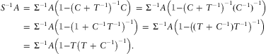 $${ {{S}^{{\rm{ - }}1}} A\, & = \,{{\rSigma }^{{\rm{ - }}1}} A\left( {{\Bbb 1}{\rm{ - }}{{{\left( {C\, + \,{{T}^{{\rm{ - }}1}} } \right)}}^{{\rm{ - }}1}} C} \right)\, = \,{{\rSigma }^{{\rm{ - }}1}} A\left( {\Bbb{1}}{\rm{ - }}{{{\left( {C\, + \,{{T}^{{\rm{ - }}1}} } \right)}}^{{\rm{ - }}1}} {{{({{C}^{{\rm{ - }}1}} )}}^{{\rm{ - }}1}} } \right) \cr & = \,{{\rSigma }^{{\rm{ - }}1}} A\left( {{\Bbb 1}{\rm{ - }}{{{\left( {{\Bbb1}\, + \,{{C}^{{\rm{ - }}1}} {{T}^{{\rm{ - }}1}} } \right)}}^{{\rm{ - }}1}} } \right)\, = \,{{\rSigma }^{{\rm{ - }}1}} A\left( {{\Bbb 1}{\rm{ - }}{{{\left( {(T\, + \,{{C}^{{\rm{ - }}1}} ){{T}^{{\rm{ - }}1}} } \right)}}^{{\rm{ - }}1}} } \right) \cr &= \,{{\rSigma }^{{\rm{ - }}1}} A\left( {{\Bbb 1}{\rm{ - }}T{{{\left( {T\, + \,{{C}^{{\rm{ - }}1}} } \right)}}^{{\rm{ - }}1}} } \right). \cr}$$
Let us calculate the last bracket, it provides
 $${ {\Bbb 1}{\rm{ - }}T{{\left( {T\, + \,{{C}^{{\rm{ - }}1}} } \right)}^{{\rm{ - }}1}} & = \,\left( {T\, + \,{{C}^{{\rm{ - }}1}} } \right){{\left( {T\, + \,{{C}^{{\rm{ - }}1}} } \right)}^{{\rm{ - }}1}} {\rm{ - }}T{{\left( {T\, + \,{{C}^{{\rm{ - }}1}} } \right)}^{{\rm{ - }}1}} \cr & = \,\left( {\left( {T\, + \,{{C}^{{\rm{ - }}1}} } \right){\rm{ - }}T} \right){{\left( {T\, + \,{{C}^{{\rm{ - }}1}} } \right)}^{{\rm{ - }}1}} \, = \,{{C}^{{\rm{ - }}1}} {{\left( {T\, + \,{{C}^{{\rm{ - }}1}} } \right)}^{{\rm{ - }}1}} \cr &= \,{{\left( {TC\, + \,{\Bbb 1}} \right)}^{{\rm{ - }}{ 1}}} \, = \,{{\left( {C\, + \,{{T}^{{\rm{ - }}1}} } \right)}^{{\rm{ - }}1}} {{T}^{{\rm{ - }}1}} \, = \,B{{T}^{{\rm{ - }}1}} . \cr}$$
We have just proved that  $$)(-->$<> {{S}^{{\rm{ - }}1}} A\, = \,{{\rSigma }^{{\rm{ - }}1}} AB{{T}^{{\rm{ - }}1}} <$>
<!--$$. Thus, (A.1) becomes
 $$f(\bixi )\, \propto \,{\rm{exp}}\left\{ {{\rm{ - }}\frac{1}{2}\left( {\bixi ^{\prime}{{S}^{{\rm{ - }}1}} \bixi {\rm{ - }}2\bixi ^{\prime}{{S}^{{\rm{ - }}1}} A\bimu } \right)} \right\}\, \propto \,{\rm{exp}}\left\{ {{\rm{ - }}\frac{1}{2} \left( {\bixi {\rm{ - }}A\bimu } \right){{S}^{{\rm{ - }}1}} \left( {\bixi {\rm{ - }}A\bimu } \right)} \right\}.$$
This completes the proof.
□
Proof of Lemma 3.3. The lemma is an immediate consequence of Theorem 3.1. Note that the linear, bijective map (3.1) only describes a relabeling of the components (permutation) and this does not change the type of the underlying distribution. The first two moments are then also a consequence of Theorem 3.1 using the linearity of the projections, see also Result 4.4 in Johnson & Wichern (Reference Johnson and Wichern1988).
□
Proof of Theorem 3.4. In view of Lemma 3.3 this is a well-known statement for multivariate Gaussian distributions, see Pestman (Reference Pestman1998), pages 427–428, or Result 4.6 in Johnson & Wichern (Reference Johnson and Wichern1988). The matrix  $$)(-->$<> {\rm{Cov}}({{\bixi }^{{{{\scr D}}^c} }} |{{\bixi }^{\scr D}} ) <$>
<!--$$ describes the Schur complement of SD in S, we also refer to Section A.5.5 in Boyd & Vandenberghe (Reference Boyd and Vandenberghe2004).
□
Proofs of Theorems 4.1 and 4.3. Note that  $$)(-->$<> {\bf {{e}}}{{^{\prime}}_{t|i,n}} {{\bixi }^{{\scr D}_{t}^{c} }} <$>
<!--$$ is a sum over components in
 $$)(-->$<> {{\bixi }^{{\scr D}_{t}^{c} }} <$>
<!--$$. From Theorem 3.4 we obtain that
 $$)(-->$<> {\bf {{e}}}^{{\rm{\prime }}}_{t|i,n}} {{\bixi }^{{\scr D}_{t}^{c} }} |{{\bixi }^{{{{\scr D}}_t}}} <$>
<!--$$ has a Gaussian distribution with posterior mean
 $$)(-->$<> {\bf {{e}}}{{^{\prime}}_{t|i,n}}\bimu _{{{\scr D}_{t}^{c} }}^{{{\rm{post}}}} <$>
<!--$$ and posterior variance
 $$)(-->$<> {\bf {{e}}}{{^{\prime}}_{t|i,n}} S_{{{\scr D}_{t}^{c} }}^{{{\rm{post}}}} {{{\bf {{e}}}}_{t|i,n}} <$>
<!--$$. Then the claims immediately follow from the properties of log-normal distributions.
□
Proof of Lemma 5.1. Because successive predictions are (Ft)t-martingales and in view of Theorem 3.4 we have
 $${\mathop{\widehat C}\nolimits^{}} _{{i,J,n}}^{{(t)}} \, = \,{\Bbb E}\left[ {\left. {{\mathop{\widehat C}\nolimits^{}} _{{i,J,n}}^{{(t\, + \,1)}} } \right|{{\scr F}_t}} \right]\, = \,{{g}_{t|i,n}}({{\scr F}_t}) {\rm{exp}}\left\{ {{\bf {{p}}}{{^{\prime}}_{t|i,n}}\bimu _{{{\scr D}_{t}^{c} }}^{{{\rm{post}}}} \, + \,\frac{1}{2}{\bf {{p}}}{{^{\prime}}_{t|i,n}}S_{{{\scr D}_{t}^{c} }}^{{{\rm{post}}}} {{{\bf {{p}}}}_{t|i,n}}} \right\}.$$
The rhs now needs to be equal to the term given in Theorem 4.1 which proves the claim.
□
Proof of Theorem 5.2. A straightforward calculation shows
 $${ {\rm{Cov}}\left( {\left. {{\mathop{\widehat C}\nolimits^{}} _{{i,J,n}}^{{(t\, + \,1)}}, {\mathop{\widehat C}\nolimits^{}} _{{l,J,m}}^{{(t\, + \,1)}} } \right|{{\scr F}_t}} \right)\, &= \,{\Bbb E}\left[ {\left. {{\mathop{\widehat C}\nolimits^{}} _{{i,J,n}}^{{(t\, + \,1)}} {\mathop{\widehat C}\nolimits^{}} _{{l,J,m}}^{{(t\, + \,1)}} } \right|{{\scr F}_t}} \right]{\rm{ - }}{\Bbb E}\left[ {\left. {{\mathop{\widehat C}\nolimits^{}} _{{i,J,n}}^{{(t\, + \,1)}} } \right|{{\cal F}_t}} \right]{\Bbb E}\left[ {\left. {{\mathop{\widehat C}\nolimits^{}} _{{l,J,m}}^{{(t\, + \,1)}} } \right|{{\scr F}_t}} \right] \cr & = \,{{g}_{t|i,n}}({{\scr F}_t}) {{g}_{t|l,m}}({{\scr F}_t}) \big ({\Bbb E}\left[ {\left. {{\rm{exp}}\left\{ {({\bf {{p}}}{{^{\prime}}_{t|i,n}}\, + \,{\bf {{p}}}{{^{\prime}}_{t|l,m}}){{{\bf {{\bixi }}}}^{{\scr D}_{t}^{c} }} } \right\}} \right|{{\scr F}_t}} \right] \cr &\quad\quad{\rm{ - }} {\Bbb E}\left[ {\left. {\rm exp}\left\{ {{\bf {{p}}}{{^{\prime}}_{t|i,n}}{{{\bf {{\bixi }}}}^{{\scr D}_{t}^{c} }} } \right\}} \right|{{\scr F}_t}} \right]{\Bbb E}\left[ {\left. {{\rm exp}\left\{ {{\bf {{p}}}{{^{\prime}}_{t|l,m}}{{{\bf {{\bixi }}}}^{{\scr D}_{t}^{c} }} } \right\}} \right|{{\scr F}_t}} \right]\big) \cr & = \,{\mathop{\widehat C}\nolimits^{}} _{{i,J,n}}^{{(t)}} {\mathop{\widehat C}\nolimits^{}} _{{l,J,m}}^{{(t)}} \left( {{\rm{exp}}\left\{ {{\bf {{p}}}{{^{\prime}}_{t|i,n}} S_{{{\scr D}_{t}^{c} }}^{{{\rm{post}}}} {{{\bf {{p}}}}_{t|l,m}}} \right\}{\rm{ - }}1} \right). \cr}$$
This proves the theorem.
□
Proof of Lemma 5.3. For the first claim we note that  $$)(-->$<> {{\bixi }^{{\scr D}_{t}^{c} }} \, = \,{{P}_{{\scr D}_{t}^{c} }}\bixi <$>
<!--$$. Thus, the linear map
 $$)(-->$<> {{P}_{{\scr D}_{t}^{c} }}:{{{\Bbb R}}^d} \rightarrow {{{\Bbb R}}^{|{\scr D}_{t}^{c} |}} <$>
<!--$$ selects all components of
 $$)(-->$<>\bixi<$>
<!--$$ which are in
 $$)(-->$<> {\scr D}_{t}^{c} <$>
<!--$$. Next, we observe that the linear map
 $$)(-->$<> {{P^{\prime}}_{{\scr D}_{t}^{c} }}:{{{\Bbb R}}^{|{\scr D}_{t}^{c} |}} \rightarrow {{{\Bbb R}}^d} <$>
<!--$$ maps the vector
 $$)(-->$<> {{\bixi }^{{\scr D}_{t}^{c} }} <$>
<!--$$ to the vector
 $${\mathop{\tilde \bixi }\limits^{}} \, = \,{{\left( {{{\xi }_{i,j,n}}{{{ 1}}_{\{ (i,j,n) \in {\scr D}_{t}^{c} \} }}} \right)}{^\prime}_{(i,j,n) \in \cal J}} \in {{{\Bbb R}}^d}, $$
i.e. all components  $$)(-->$<> (i,j,n)\, \notin \,{\scr D}_{t}^{c} <$>
<!--$$ are set equal to 0. This implies that the linear map
 $$)(-->$<> ({{P^{\prime}}_{{\scr D}_{t}^{c} }}{{P}_{{\scr D}_{t}^{c} }}):{{{\Bbb R}}^d} \rightarrow {{{\Bbb R}}^d} <$>
<!--$$ exactly selects all the components that are in
 $$)(-->$<> {\scr D}_{t}^{c} <$>
<!--$$, i.e.
 $$({{P^{\prime}}_{{\scr D}_{t}^{c} }}{{P}_{{\scr D}_{t}^{c} }}) \bixi \, = \,{\mathop{\tilde \bixi }\limits^{}} \, = \,{{\left( {{{\xi }_{i,j,n}}{{{ 1}}_{\{ (i,j,n) \in {\scr D}_{t}^{c} \} }}} \right)}^{\prime}_{(i,j,n) \in {\cal J}}}\, \in \,{{{\Bbb R}}^d} .$$
If we finally apply the linear map  $$)(-->$<> {{P}_{{{{\scr D}}_{t\, + \,1}}}}\,:\,{{{\Bbb R}}^d} \rightarrow {{{\Bbb R}}^{|{{{\scr D}}_{t\, + \,1}}|}} <$>
<!--$$ we see that
 $$({{P}_{{{{\scr D}}_{t\, + \,1}}}}{{P^{\prime}}_{{\scr D}_{t}^{c} }}{{P}_{{\scr D}_{t}^{c} }}) \bixi \, = \,{{P}_{{{{\scr D}}_{t\, + \,1}}}} {\mathop{\tilde \bixi }\limits^{}} \, = \,{{\left( {{{\bixi }_{i,j,n}}{{{ 1}}_{\{ (i,j,n) \in {\scr D}_{t}^{c} \} }}} \right)}^{\prime}_{(i,j,n) \in {{{\scr D}}_{t\, + \,1}}}}\, \in \,{{{\Bbb R}}^{|{{{\scr D}}_{t\, + \,1}}|}}, $$
thus, we keep the values of the components  $$)(-->$<> (i,j,n)\, \in \,{{{\scr D}}_{t\, + \,1}}\, \cap \,{\scr D}_{t}^{c} <$>
<!--$$ and all components in
 $$)(-->$<> {{{\scr D}}_{t\, + \,1}}\backslash {\scr D}_{t}^{c} <$>
<!--$$ are set equal to 0 which exactly is equal to
 $$)(-->$<> {{B}_{t\, + \,1}}{{\bixi }^{{{{\scr D}}_{t\, + \,1}}}} <$>
<!--$$.
For the second claim we observe (using the first statement) that
 $$({{P^{\prime}}_{{{{\scr D}}_{t\, + \,1}}}}{{P}_{{{{\scr D}}_{t\, + \,1}}}}{{P^{\prime}}_{{\scr D}_{t}^{c} }}) {{\bixi }^{{\scr D}_{t}^{c} }} \, = \,{{P^{\prime}}_{{{{\scr D}}_{t\, + \,1}}}}\,{{B}_{t\, + \,1}}{{{\bf {{\xi }}}}^{{{{\scr D}}_{t\, + \,1}}}} \, = \,{{\left( {{{\bixi }_{i,j,n}}{{{ 1}}_{\{ (i,j,n)\, \in \,{\scr D}_{t}^{c} \cap {{{\scr D}}_{t\, + \,1}}\} }}} \right)}^{\prime}_{(i,j,n)\, \in \,{\cal J}}}\, \in \,{{{\Bbb R}}^d} .$$
This implies
 $$ ({{P}_{{\scr D}_{t}^{c} }}{{P^{\prime}}_{{{{\scr D}}_{t\, + \,1}}}}{{P}_{{{{\scr D}}_{t\, + \,1}}}}{{P^{\prime}}_{{\scr D}_{t}^{c} }}) {{\bixi }^{{\scr D}_{t}^{c} }} \, = \,{{P}_{{\scr D}_{t}^{c} }}{{\left( {{{\bixi }_{i,j,n}}{{{ 1}}_{\{ (i,j,n) \in {{{\scr D}}_{t\, + \,1}}\} }}} \right)}^{\prime}_{(i,j,n) \in {\scr D}_{t}^{c} }}\, \in \,{{{\Bbb R}}^{|{\scr D}_{t}^{c} |}} . $$
Thus,  $$)(-->$<> ({{P}_{{\scr D}_{t}^{c} }}{{P^{\prime}}_{{{{\scr D}}_{t\, + \,1}}}}{{P}_{{{{\scr D}}_{t\, + \,1}}}}{{P^{\prime}}_{{\scr D}_{t}^{c} }}) {{\bixi }^{{\scr D}_{t}^{c} }} <$>
<!--$$ considers all components of
 $$)(-->$<> {{\bixi }^{{\scr D}_{t}^{c} }} <$>
<!--$$ which become observable at time t + 1, i.e. for which i + j = t + 1, and the other ones are set equal to 0. But this implies the claim because
 $${\bf {{e}}}{{^{\prime}}_{t|i,n}} ({{P}_{{\scr D}_{t}^{c} }}{{P^{\prime}}_{{{{\scr D}}_{t\, + \,1}}}}{{P}_{{{{\scr D}}_{t\, + \,1}}}}{{P^{\prime}}_{{\scr D}_{t}^{c} }}) {{\bixi }^{{\scr D}_{t}^{c} }} \, = \,\mathop{\sum}\limits_{j\, = \,t{\rm{ - }}i\, + \,1}^J {{\bixi }_{i,j,n}}{{ 1}_{\{ i\, + \,j\, = \,t\, + \,1\} }}\, = \,{{\bixi }_{i,t\, + \,1{\rm{ - }}i,n}}.$$
Observed general liability (GL) data Ci,j,n with i + j ≤ I = 14 and n = 1. The vector  $$)(-->$<> {{\bimu }_n} = ({{\mu }_{0,n}}, \ldots, {{\mu }_{J,n}})^{\prime} <$>
<!--$$ denotes the prior mean of parameter vector Θ that corresponds to sub-portfolio n = 1,
 $$)(-->$<> {{\bisigma }_n} = ({{\sigma }_{0,n}}, \ldots, {{\sigma }_{J,\,n}})^{\prime} <$>
<!--$$ denotes the standard deviation parameters implied from
 $$)(-->$<>\rSigma<$>
<!--$$ for sub-portfolio n = 1, and for the prior covariance matrix we choose T = τ 2
 $$)(-->$<>\Bbb {1}<$>
<!--$$ with τ = 1.

Observed motor third party liability (MTPL) data Ci,j,n with i + j ≤ I = 14 and n = 2. The vector  $$)(-->$<> {{\bimu }_n}\, = \,({{\mu }_{0,n}}, \ldots, {{\mu }_{J,n}})^{\prime} <$>
<!--$$ denotes the prior mean of parameter vector Θ that corresponds to sub-portfolio n = 2,
 $$)(-->$<> {{\bisigma }_n}\, = \,({{\sigma }_{0,n}}, \ldots, {{\sigma }_{J,n}})^{\prime} <$>
<!--$$ denotes the standard deviation parameters implied from
 $$)(-->$<>\rSigma<$>
<!--$$ for sub-portfolio n = 2, and for the prior covariance matrix we choose T = τ 2
 $$)(-->$<>\Bbb {1}<$>
<!--$$ with τ = 1.

This finishes the proof of the lemma.
□