Introduction
The moderate to high values of heritability estimated for gestation length during last decade (Hanenberg et al., Reference Hanenberg, Knol and Merks2001; Serenius et al., Reference Serenius, Sevón-Aimonen, Kause, Mäntysaari and Mäki-Tanila2004; Nguyen et al., Reference Nguyen, McPhee and Wade2006) have increased its importance as a potential breeding goal to improve the efficiency of the sow per time unit. On the other hand, an increase in gestation length has been related with an improved piglet vitality at birth and the reduced stillbirths (Zaleski and Hacker, Reference Zaleski and Hacker1993; Leenhouwers et al., Reference Leenhouwers, Van der Lende and Knol1999; Knol et al., Reference Knol, Leenhouwers and Van der Lende2002). There is substantial controversy on the relation between gestation length and incidence of splay leg piglets (Sellier and Ollivier, Reference Sellier and Ollivier1982; Van der Heyde et al., Reference Van der Heyde, De Mets, Porreye, Henderickx, Calus, Bekaert and Buysse1989), and the reduction of gestation length has been related with an increase of the farrowing duration (Van der Heyde et al., Reference Van der Heyde, De Mets, Porreye, Henderickx, Calus, Bekaert and Buysse1989). As a whole, gestation length could be viewed as a useful indicator of piglet viability and plays an important role in pig reproduction. Given the substantial relation between gestation length and piglet viability and survival, it is interesting to improve our knowledge about its genetic background and to evaluate the benefit of marker-related strategies of selection.
Genome scans for quantitative trait loci (QTL) in F2 crosses exploit the genetic divergence between two breeds to detect chromosomal regions linked to traits of interest. Within this context, we generated an Iberian × Meishan F2 intercross, an important genetic resource for QTL detection because both breeds were produced from independent domestication processes. Indeed, there is substantial evidence that the Iberian breed has not been introgressed with Asian alleles (Alves et al., Reference Alves, Óvilo, Rodríguez and Silió2003), a current influence in the greater part of the European breeds (Haley and Lee, Reference Haley and Lee1993). Within this context, the aim of our research was to perform a genome scan to detect QTL related with gestation length in order to go deeply in the knowledge of the genetic basis of this trait.
Material and methods
Experimental data source
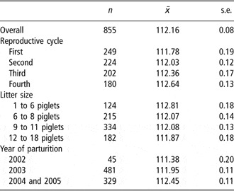
Data on gestation length were obtained from an F2 experimental design for detecting QTL for reproductive traits in pigs. A total of 855 records of gestation length from 249 Iberian × Meishan F2 sows were recorded in Nova Genètica experimental farm of Solsona (Lleida, Spain) between October 2002 and January 2005 (Table 1). Those sows were generated from 97 F1 gilts mated with 8 F1 boars, and the F0 generation composed of 3 Guadyerbas Iberian boars (CIA El Dehesón del Encinar, Toledo, Spain) and 18 Meishan sows (INRA, GEPA experimental unit, Surgères, France).
Summary of the gestation length data set

Sows followed a standard management during the four reproductive cycles. F2 sows were mated by AI with semen of Large White boars, penned in standard gestation crates during pregnancy, and transferred to climate-controlled farrowing rooms (24°C) 10 days before parturition. After delivery, the length of the lactation period was 22 to 25 days. Feeding of sows was restricted during the gestation period (9.2 MJ net energy (NE), 13.5% crude protein (CP) and 0.48% lysine), and ad libitum during lactation (9.8 MJ of NE, 17.5% CP and 0.82% lysine).
Genotyping
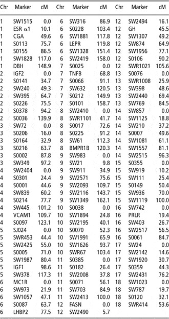
Genomic DNA of purebred F0 individuals, F1 reproducers and 249 F2 sows was extracted from blood or tail tissue using standard protocols (Gentra Systems, Minneapolis, MN, USA). All the individuals were genotyped for 109 microsatellites and 10 single-nucleotide polymorphisms (SNPs; Table 2). The microsatellite PCR products were analysed with the Genescan 3.7 software (Applied Biosystems, Warrington, UK) in a capillary electrophoresis equipment with fluorescent detection (ABI PRISM 310 Genetic Analyser; Applied Biosystems, Foster City, CA, USA). The analysis of SNPs was performed by primer extension for the DBH (Tomás et al., Reference Tomás, Casellas, Ramírez, Muñoz, Noguera and Sánchez2006b), VCAM1 (Ramírez et al., Reference Ramírez, Blanch, Amills, Noguera and Sánchez2003), BMPR1B (Tomás et al., Reference Tomás, Casellas, Ramírez, Pérez-Enciso, Rodríguez, Noguera and Sánchez2006a), PRLR (Tomás et al., Reference Tomás, Frigo, Casellas, Ramírez, Óvilo, Noguera and Sánchez2006c) and MTNR1A (Ramírez et al., 2005) genes, and by PCR-restriction fragment length polymorphism (RFLP) for the ESR (Short et al., Reference Short, Rothschild, Southwood, McLaren, De Vries, Van der Steen, Eckardt, Tuggle, Helm, Vaske, Mileham and Plastow1997), GH and FASN (Rodríguez et al., Reference Rodríguez, Tomás, Alves, Ramírez, Arqué, Muñoz, Barragán, Varona, Silió, Amills and Noguera2005), LHBP2 (Muñoz et al., 2005) and MC1R (Kijas et al., Reference Kijas, Wales, Törnsten, Chardon, Moller and Andersson1998) genes. Linkage analysis was carried out by using the CRI-MAP 2.4 software (Green et al., 1990). Markers provided coverage of the 18 autosomes, with an average marker interval of 17.4 cM (sex-averaged map distance).
Markers genotyped and position (cM) for each autosomal pig chromosome (Chr)

Trait and operational model
Gestation length was defined as the days from first fertile insemination to farrowing. Systematic effects considered were order of parity of the sow with four levels according to the four first parturitions, litter size including piglets born alive and stillbirths (categorized as <6, 6 to 8, 9 to 11 and >11 piglets), and year of farrowing (2002, 2003 and 2004). Note that only two deliveries occurred in January 2005 and they were assigned to the preceding year (see Table 1 for an extensive summary of the data set). Additive and dominant effects of the QTL were modelled following Haley and Knott (Reference Haley and Knott1992). The probabilities of each QTL genotype at positions throughout the pig genome were calculated with the QTLexpress software (Haley and Knott, Reference Haley and Knott1992). Two random sources of variation were included in the model, the permanent environmental and the additive genetic effect attributable to each sow.
Calculation of the empirical Bayes factor
Consider the following model with QTL effects (model QTL):

where y contains n phenotypic records, X1, Xλ, Z1 and Z2 are the incidence matrices of systematic (b), QTL (q), permanent environmental (p) and additive genetic (a) effects, and e is the vector of residuals. In order to reduce the number of tests performed, QTL location within chromosome (λ) is included as an additional unknown parameter in our mixed model and thus, values in Xλ depends on λ. Note that q is a column vector composed by the additive (α) and dominant effect (δ) of the QTL (q′ = [α δ]) at a given chromosomal location (by cM), and it reduces to a scalar element if δ is not considered. Following a standard Bayesian development, the joint distribution of model QTL is
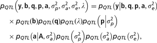
where A is the numerator relationship matrix, and  and
 are the permanent environmental, additive genetic and residual variances, respectively. The conditional distribution of y is assumed to be normally distributed:

with Ie being an identity matrix with dimension n × n. Permanent environmental and additive genetic effects are assumed normally distributed ( and
 , respectively), and prior distributions for variance components and systematic effects are stated as inverted scaled χ 2 distributions and flat distributions, respectively (see Varona et al., Reference Varona, García-Cortés and Pérez-Enciso2001). Within chromosome, the location of the QTL (λ) is assumed by cM with an a priori uniform distribution:

where L is the length of the chromosome. Finally, our empirical Bayes factor (BF) deviates from the procedure of Varona et al. (Reference Varona, García-Cortés and Pérez-Enciso2001) in the prior distributions for QTL effects. They are assumed flat:
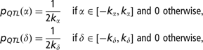
with K α and K δ being the maximum value of α and δ, defined as the extreme situation when all the phenotypic variance ( ) of gestation length is accounted by α or δ. Following Falconer and Mackay (Reference Falconer and Mackay1996) and Spencer (Reference Spencer2002), K α and K δ can be obtained as

where  , the expected frequency of both QTL alleles in an F2 population. As is mentioned in previous lines, preliminary information from gestation length data was required to construct P QTL (α) and P QTL (δ) and consequently, our model must be viewed as an empirical Bayesian model (Carlin and Louis, Reference Carlin and Louis1996). This provides appropriate bounds for α and δ within the parametric space, and allows for an easy construction of the BF as is described below.
The null-hypothesis model is the no-QTL model (model 0), with the following joint distribution of records and parameters:

We can assume that the likelihood of model 0 is

and prior distributions for the remaining parameters are identical to the prior distributions of model QTL.
Following García-Cortés et al. (Reference García-Cortés, Cabrillo, Moreno and Varona2001) and Varona et al. (Reference Varona, García-Cortés and Pérez-Enciso2001), only the analysis with the complex model (model QTL) is required to calculate the empirical BF between model QTL and model 0 (BF QTL, 0),

although additional assumptions are required to account for multiple testing (see Appendix). Note that P QTL (q = 0) equals to (4K αK δ)−1 for an additive and dominant QTL, whereas it reduces to (2K α)−1 if the dominance deviation is not accounted for. With the exception of λ, all parameters in model QTL were updated by Gibbs sampling (Gelfand and Smith, Reference Gelfand and Smith1990). Following Varona et al. (Reference Varona, Gómez-Raya, Rauw, Ovilo, Clop and Noguera2005), a Metropolis–Hastings step (Hastings, Reference Hastings1970) was used to obtain autocorrelated samples of λ, with a uniform proposal distribution centred at the current value of λ and covering 50 cM. It provided an acceptance rate greater than 20% in all chromosomes. The analyses were performed twice at each chromosome, with q defined as q′ = [α 0] or q′ = [α δ] (see Appendix for a straightforward comparison between both models). For each analysis, five independent chains were launched with different starting value for λ. Each chain had a total of 500 000 iterations and the first 50 000 were discarded as burn-in (Raftery and Lewis, Reference Raftery and Lewis1992). All correlated samples were used to calculate the posterior distributions using the ergodic property of the chain (Gilks et al., Reference Gilks, Richardson and Speigelhalter1996).
Results and discussion
Taking García-Cortés et al. (Reference García-Cortés, Cabrillo, Moreno and Varona2001) and Varona et al. (Reference Varona, García-Cortés and Pérez-Enciso2001) as starting point, we developed an empirical new variant of the BF between nested models to detect QTL. This approach models QTL parameters as systematic effects with appropriate parametric bounds conditioned by the phenotypic variance. In general, BF methodology suffers from disadvantages due to its complexity of computation in complex models or its strong dependence on the assumed prior distributions (Kass and Raftery, Reference Kass and Raftery1995). Notwithstanding, the BF described by Varona et al. (Reference Varona, García-Cortés and Pérez-Enciso2001) shows an important advantage in terms of dependence to the prior distributions for all parameters, with the only exception of the boundary variables, because they are the same in both competing models and then they are cancelled in the final calculation. In our case, prior distributions for QTL effects have been assumed flat within the rank of plausible values, with a low influence in posterior distributions.
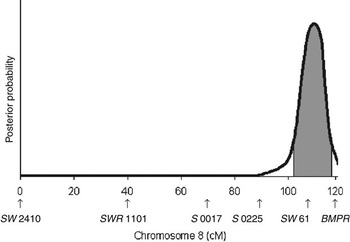
Historically, the analyses of QTL have been stated as a typical example of multiple testing, increasing the probability of false-positives and unrealistic conclusions (Churchill and Doerge, Reference Churchill and Doerge1994). Since a Bayesian point of view, numerous approaches have been proposed (Scott and Berger, 2003) although a key point in all cases is the number of tests carried out. The inclusion of λ (location of the QTL) as an unknown parameter in the model substantially reduces the number of independent tests performed in each chromosome. This approach allows for a straightforward detection of QTL within each chromosome, avoiding corrections for multiple testing if a single chromosome is analysed. If more than one QTL are located in the same chromosome, a multi-modal posterior distribution of λ is expected, and the empirical BF described above must be appropriately adapted to account for this peculiarity, e.g. reversible jump sampling (Stephens and Fisch, Reference Stephens and Fisch1998). Nevertheless, only three chromosomes showed evidences of QTL affecting gestation length in our population and, all of them provided a unimodal posterior distribution of λ (see Figure 1 as example). A separate analysis by chromosome allows for faster mixing properties of the Monte Carlo Markov chain of λ, and still implies a huge reduction in multiple testing. Within this context, posterior odds can be viewed as a useful Bayesian tool to determine significant evidences depending on our a priori knowledge. It is not straightforward to define a standard prior odds as a general rule in QTL analyses, and appropriate prior odds must be defined in each case. Obviously, it implies a certain degree of arbitrariness, although several plausible values can be easily stated to verify the obtained results under a wider range of suitable scenarios.
Posterior density of quantitative trait loci (QTL) location in chromosome 8 (highest posterior density region at 95% is grey coloured).

Gestation length averaged 112.16 days (±0.08 days) in our F2 crossbred population (Table 1), a value smaller than the ones described in Asian pig breeds crossed with West-type breeds (113.0 to 113.7 days; Young, Reference Young1995 and Reference Young1998) as well as in West-type populations (113.5 to 114.5 days; Cassady et al., Reference Cassady, Young and Leymaster2002; Leenhouwers et al., Reference Leenhouwers, Wissink, Van der Lende, Paridaans and Knol2003), and clearly shorter than the 116.1 days reported by Moeller et al. (Reference Moeller, Goodwin, Johnson, Mabry, Baas and Robinson2004). Modal estimates of variance components for gestation length were 0.67, 1.16 and 3.45 for additive genetic, permanent environmental and residual variances, respectively. Unfortunately, data from F0 generation were not available for the discrimination between additive variances from the parental populations and the segregation variance (Birchmeier et al., Reference Birchmeier, Cantet, Fernando, Morris, Holgado, Jara and Santos-Cristal2002) and, in addition, genetic components related to dominance and linkage disequilibrium between loci can be absorbed by the additive genetic variance in an F2 design. Within this context, we must be cautious with the heritability provided by the current analysis (h 2=0.13). This moderate value contrasts with the high heritabilities reported by Hanenberg et al. (Reference Hanenberg, Knol and Merks2001) and Cassady et al. (Reference Cassady, Young and Leymaster2002), although it is similar to the one described by Nguyen et al. (Reference Nguyen, McPhee and Wade2006).
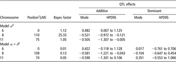
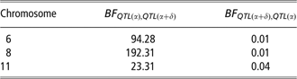
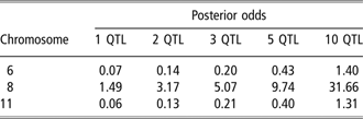
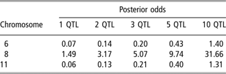
The whole-genome scan suggested the presence of additive QTL affecting gestation length in pig chromosomes 6, 8 and 11 (Table 3). The additive QTL in chromosome 8 gave strong evidence following Jeffreys (Reference Jeffreys1961; 10<BF ⩽ 31.62) whereas QTL in chromosomes 6 and 11 did not worth more than a bare mention (1<BF ⩽ 3.16) (Table 3). The joint analysis of additive and dominant QTL effects reduced BF. The models with pure-additive QTL were preferable, with strong (chromosome 11), very strong (chromosome 6) and decisive (chromosome 8) evidences (Table 4). After correcting for multiple testing, posterior odds are shown in Table 5. They suggested that, although QTL in chromosomes 6 and 11 cannot be completely discarded under less-conservative prior odds, only the QTL in chromosome 8 must be quoted. The PO QTL,0 for this QTL reached higher than 1 estimates when the a priori expected number of QTL was 1 or greater, whereas QTL in chromosome 6 and 11 had posterior odds clearly lower or close to 1. The posterior odds draws a more stringent scenario under multiple testing and suggests that there is a QTL on gestation length in pig chromosome 8, it requiring future analyses to confirm its effects and magnitude.
Results of quantitative trait loci detection for gestation length

†Mode.
‡Model with additive quantitative trait loci (QTL) effect and without dominance deviation.
§Model with additive and dominant QTL effects.
Empirical Bayes factor between QTL with and without dominant effect
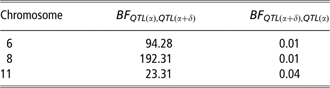
BF QTL(α), QTL(α + δ): empirical Bayes factor (BF) of the quantitative trait loci (QTL) with additive effects against the QTL with additive and dominants effects.
BF QTL(α + δ), QTL(α): empirical Bayes factor of the QTL with additive and dominant effects against the QTL with additive effects.
Posterior odds (additive quantitative trait loci (QTL) v. no-QTL) depending on the a priori expected number of QTL
A graphical representation of results for chromosome 8 is shown in Figure 1. The mode of the QTL location on chromosome 8 was placed at 110 cM, close to the marker SW61, with the highest posterior density region at 95% ranged between 103 and 118 cM (Figure 1). The joint analysis of additive and dominant effects reduced the empirical BF (Tables 3 and 4), with a slight change in the modal estimate of λ (109 cM). It can be related with a non-significant influence of the dominant deviation of the QTL, given that its higher posterior density at 95% included the null estimate (Table 3). Moreover, the empirical BF between the model with an additive QTL against the model with an additive and dominant QTL clearly favoured the first one, it being 193 times more probable (Table 4). Interestingly, the pig homologue of the Booroola fecundity gene (BMPR1B), previously related with gilt prolificacy at first parturition (Tomás et al., Reference Tomás, Casellas, Ramírez, Pérez-Enciso, Rodríguez, Noguera and Sánchez2006a), was located at the bound of that interval (118 cM), although it seems unlikely that BMPR1B was the gene responsible for the gestation length QTL reported here. The additive fraction of the phenotypic variance explained by this QTL was around 3.4% (assuming modal estimates). No comparable QTL on gestation length have been mapped in chromosome 8, although QTL for closely related reproductive traits were detected in this chromosome (e.g. prenatal survival (King et al., Reference King, Jiang, Gibson, Haley and Archibald2003); ovulation rate (Rathje et al., Reference Rathje, Rohrer and Johnson1997); uterine capacity (Rohrer et al., Reference Rohrer, Ford, Wise, Vallet and Christenson1999)). To the best of our knowledge, the previous research of Wilkie et al. (Reference Wilkie, Paszek, Beattie, Alexander, Wheeler and Schook1999) in a Meishan × Yorkshire cross described the first QTL for gestation length in chromosome 9. Our results did not allow confirmation of this QTL because significant results were not observed in this chromosome. Nevertheless, these differences could be due to the different breeds used in each F2 cross.
Conclusion
The genetic basis of the main components of gestation length in sow has been investigated in an experimental Iberian × Meishan F2 intercross. An empirical BF has been developed to scan QTL and it provided evidences of a QTL in chromosome 8, with an additive effect favourable to the Meishan allele of approximately half a day.
Acknowledgements
Financial support was provided by Ministerio de Ciencia y Tecnología, Spain (Grants AGL2000-1229-C03 and AGL2004-08368-C03/GAN). The authors are indebted to the staff of Nova Genètica, in particular to E. Ramells, F. Marquez, R. Malé and F. Rovira for cooperating in the experimental protocol, to M. Arqué and I. Riart (IRTA) and J. C. Caritez (INRA) for their technical support, and to J. P. Bidanel (INRA) for their help and collaboration. The authors gratefully acknowledge the contributions of the INRA (France) and the CIA El Dehesón del Encinar (Spain) for providing the purebred Meishan sows and Iberian boars, respectively.
Appendix
Comparison between pure-additive QTL and additive and dominant QTL
Take BFQTL(α),0 as the empirical Bayes factor (BF) between a pure-additive QTL model (QTL(α)) and the no-QTL model (Model 0), and BFQTL(α + δ),0 as the empirical BF between an additive and dominant QTL model (QTL(α + δ)) and the no-QTL model. Note that both QTL(α) and QTL(α + δ) are contrasted against model 0 and then, the empirical BF between the additive QTL and the additive and dominant QTL can be easily obtained as

Correction for multiple testing
From the standard definition of BF (Kass and Raftery, Reference Kass and Raftery1995):

where POQTL,0 is the posterior odds between model QTL and model 0 and PrOQTL,0 is the prior odds. POQTL,0 can be viewed as a weighted BF accounting for a more realistic a priori probability for both models under multiple testing. We could assume that the a priori probability of both model QTL and model 0 could be appropriately defined depending on our degree of belief on the expected number of QTL before the analysis. In the standard development of the empirical BF described above, we assumed that the prior odds were 1 and the a priori probability for the QTL model and the no-QTL model were both 0.5 at each chromosome, providing an a priori expected number of QTL of 9. Obviously, it is an unrealistic assumption and a more-conservative criterion must be taken. If we initially expect n QTL, the a priori probability of the QTL model (P QTL) and the no-QTL model (P 0) at each chromosome becomes n/18 and (18 − n)/18, respectively. Posterior odds can be easily obtained as

which provides a straightforward correction for multiple testing.