

Introduction and Motivation
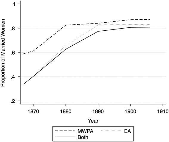
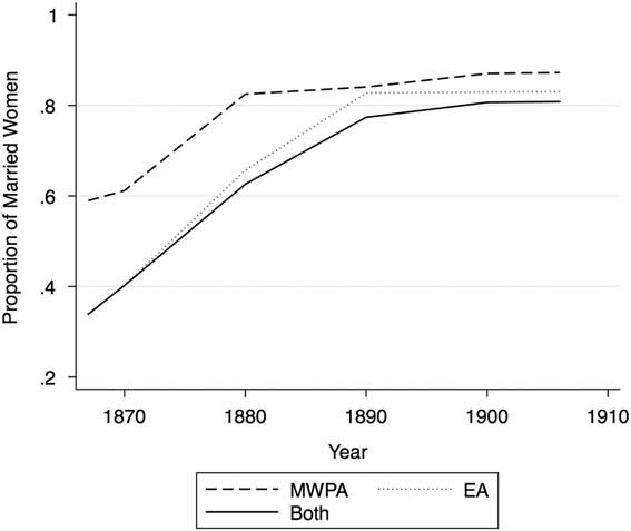
The Married Woman’s Property Acts and Earnings Acts (hereafter MWPAs and EAs) were statutes that expanded married women’s rights to their property and labor market earnings. Prior to these laws, most married women were femes covert, or “covered women,” under the common law. This meant that, upon entering the marriage contract, the wife transferred her property to her husband, who had exclusive ownership and control rights over it. Any property acquired by her during marriage also became her husband’s. While the first set of MWPAs was mainly enacted in the 1830s and 1840s to protect the wife’s property from her husband’s creditors, later “waves” of legislation established separate estates for married women. Inspired by the dramatic shift away from coverture that was put into motion by these laws, many scholars have analyzed whether the laws increased girls’ noncompulsory education, women’s innovation, the distribution of wealth in the household, and labor supply. Figure 1 shows that the percentage of married women residing in a state with an MWPA rose from about 60 percent in 1867 to more than 80 percent in 1906, with an even greater increase in the proportion of married women covered by both laws (from less than 40 percent in 1867 to close to 80 percent in 1906).
Married women residing in a state with an MWPA from 1867 to 1906.
The question that this article seeks to answer is whether the laws also affected divorce rates. In an article titled “Re-Assessing the Married Woman’s Property Acts,” historian Carole Shammas noted that, with the MWPAs, “[w]ives seeking divorce now had a much surer claim to the property they brought to a marriage. The late nineteenth century witnessed a more rapid increase in the divorce rate . . . than at any other time in U.S. history” (Shammas Reference Shammas1994: 25–26). Shammas then suggested that the MWPAs contributed to (but do not completely explain) the rise in divorce rates. Some contemporary polemics also identified a possible connection between the property acts and divorce rates (Smith Reference Smith1884). The question that we attempt to answer is whether there is a theoretical framework and empirical evidence to support Shammas’s claim regarding both the MWPAs and the EAs.
To test the hypothesis that the MWPAs and EAs contributed to the rise in divorce rates, we use two sources of data from the late nineteenth and early twentieth century to construct a single 40-year period series of divorce rates from 1867 to 1906. Looking ahead to the main results, we find that the property acts significantly increased divorce rates but that the EAs neither increased nor decreased them over the long term. We also find that other explanations for the rise in divorce rates (such as divorce law, economic development, and foreign immigration) do not have empirical support, while there is evidence to support urbanization and age structure (namely the presence of a younger population) as a cause of higher divorce rates. We account for the dynamic effects of the laws and find that divorce rates were not rising prior to an MWPA, and that the laws took at least five years before they began to affect divorce rates. Finally, we provide additional evidence from court cases that make a connection between the property acts and divorce cases, showing how the property acts were used to defend against men who claimed rights over their ex-wife’s property.
After a discussion of the literature on the MWPAs, EAs, and the history of divorce in the nineteenth-century United States, we develop a theoretical framework to understand how women’s income is expected to affect household bargaining and the probability of divorce. We then describe the data used in the analysis and present our regression model. Finally, we present our results and discuss them in the context of alternative explanations for rising divorce rates.
Literature Review
In this section, we discuss the historical background behind the MWPAs and EAs; the research on their economic and social effects; and the major causes behind the rise in divorce rates in the second half of the nineteenth century, according to the historiography. Chused (Reference Chused1983) observed that there were three waves of MWPA and EA legislation. The first wave, in the late 1830s and 1840s, arose along with the early women’s rights movement and represented the first “chipping away” at coverture law. The first wave was mostly concerned with protecting a married woman’s property from her husband’s creditors. Thus, these laws were more reactive than proactive. They were also conservatively written, strictly interpreted by the courts, and, for these reasons, were the subject of scholarly criticism about their potential for causing social and economic change (Basch Reference Basch1979, Reference Basch1982). For example, Basch (Reference Basch1979) analyzed the 1848 MWPA in New York and found that courts declared the law unconstitutional and found other ways of limiting its scope. The second and third waves refer to the refinement of the early statutes through the proactive establishment of separate estates (in the second wave) and rights to earnings (in the third wave) that gave full ownership and control rights to married women, instead of simply protecting their property from their husbands’ creditors (Chused Reference Chused1983: 1398).
The laws passed during the second and third waves are the ones that we focus on in this article because they were the laws responsible for establishing ownership and control rights over a married woman’s property and earnings. Because the role of the women’s rights movement in the passage of the MWPAs is confined mostly to the first wave, the effects of the laws can be analyzed at a distance from the immediate influence that these movements had on social dynamics, including those in the household. As another check on whether social changes might have been primarily responsible for both the rise in divorce rates and the passage of the MWPAs and EAs, we will conduct a dynamic analysis in our empirical work to assess whether divorce rates were already increasing prior to the passage of an MWPA or EA.
Researchers have come to mixed conclusions about the social and economic significance of the MWPAs and EAs. Khan (Reference Khan1996) first analyzed the impact of the laws on innovation and argued that they spurred technological development by providing women with the economic incentives to invest in their human capital. Later work by Geddes et al. (Reference Geddes, Lueck and Tennyson2012) found that they increased girls’ noncompulsory schooling. Roberts (Reference Roberts2014) did not find that they had a significant impact of the laws on married women’s labor force participation, and most recently, McDevitt and Irwin (Reference McDevitt and Irwin2017) argued that they were not primarily responsible for the narrowing of the gender wealth gap in the nineteenth century.
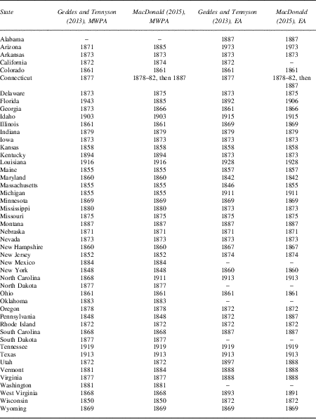
Assessment of the effects of the laws is dependent on correctly specifying when an effective MWPA or EA was enacted—a task that is complicated by the fact that the statutes sometimes contained loopholes or left out certain types of property ownership (like the rent derived from property) from the ambit of women’s rights. Because the legislative record is unclear, some early studies, such as Khan (Reference Khan1996) and Geddes and Lueck (Reference Geddes and Lueck2002), used their own dates of passage. This inconsistency was addressed by Geddes and Tennyson (Reference Geddes and Tennyson2013), who developed a definitive set of dates of passage for both the property acts and EAs. They argued that if a law established ownership rights only, it was not sufficient because property rights refer to the ability to control or manage the income derived from property. Thus, they based their criteria on whether an act established both ownership and control rights over property and earnings. Their dates of passage are considered the definitive assessment of the timing of the laws from a legislative perspective.
Courts also played a role in complicating the laws’ effects, and court rulings provide additional information about which laws were most relevant (Basch Reference Basch1979; Siegel Reference Siegel1994, Reference Siegel1995). Thus, a judicial perspective adds even more information about the effectiveness of an MWPA or EA that can be used to correctly define a date of passage. MacDonald (Reference MacDonald2015) analyzed records of court cases in digitized legal databases that referenced each state’s MWPA and EA and compared the judicial record to the dates of passage reported in Geddes and Tennyson (Reference Geddes and Tennyson2013). MacDonald (Reference MacDonald2015) concluded that while most of Geddes and Tennyson’s dates of passage remained unrevised, there were a few states where there were differences between the reported date of passage in the legislature and the effective date of passage from a judicial perspective. For example, in MacDonald (Reference MacDonald2015), Connecticut’s date of passage was revised because a review of court cases in that state led to the discovery that the MWPA was passed a year later (in 1878 instead of 1877) and was repealed in 1882, only to be reinstated in 1887. In North Carolina, a court case was found noting that the 1868 MWPA required that ownership or control rights could be granted only by the husband’s consent. The actual North Carolina MWPA was not passed until 1911. Due to these discrepancies, both sets of dates of passage are reported in table 1, though only the MacDonald (Reference MacDonald2015) dates of passage will be used for the empirical analysis in this article.
Dates of passage of the MWPAs and EAs

Sources: Geddes and Tennyson (Reference Geddes and Tennyson2013) and MacDonald (Reference MacDonald2015).
Note: A dash (–) indicates that no date was recorded for that state based on the available evidence. MacDonald (Reference MacDonald2015) dates of passage are based on Geddes and Tennyson (Reference Geddes and Tennyson2013), but they are revised based on the former author’s court case research, which occasionally found that the courts used a different law in ruling on married women’s property cases. The laws are assumed to take effect the year in which they are passed.
Finally, this article contributes to the history of the rise in divorce rates in the second half of the nineteenth century. The main reasons for the rise in divorce rates documented in the literature are attitudinal changes, urbanization, a younger population, foreign immigration, and the expansion of women’s economic opportunities and the resulting increase in labor force participation (Furstenberg 1994; Plateris Reference Plateris1973; Strow and Strow Reference Strow and Strow2006; Teachman et al., Reference Teachman, Tedrow and Hall2006). Ruggles (Reference Ruggles1997) explored some of these reasons quantitatively and found a positive relationship between increased labor market opportunities for women (as well as the lack of labor market opportunities for men) and increases in the probability of divorce beginning around 1880. See also Ruggles (Reference Ruggles2015) for an elaboration of the significance of labor market opportunities in explaining divorce rates throughout US history. While Ruggles (Reference Ruggles1997) argued that attitudinal changes could have produced both higher labor force participation and marital instability, he argued that these changes are likely a function of economic development: As women engaged more with the labor market, economic independence and individualism increased the rate of divorce. Ruggles (Reference Ruggles1997) also found that urbanization (measured by the nonagricultural employment share) increased the probability of divorce, consistent with other historical studies of the rise in divorce rates (see later in this section—and in the early to mid-nineteenth century, see Schultz Reference Schultz1984, Reference Schultz1986, Reference Schultz1990). Preston and McDonald (Reference Preston and McDonald1979) argued that a decrease in the unemployment rate during this period was associated with an increase divorce rates by reducing economic strain on families that made divorce less costly. Macroeconomic factors were not as significant as urbanization and the expansion of labor market opportunities for women.
Other historians have examined the social context behind the rise in divorce rates during this period. O’Neill (Reference O’Neill1965) argued that the attempts in the 1880s to amend divorce law to make divorces harder to achieve were reflective of a backlash against the “revolution in morals represented by mass divorce” (O’Neill Reference O’Neill1965: 217). Consistent with a thesis elaborated on later in this article, O’Neill also noted that the laws did not slow the upward trend in divorce rates into the early twentieth century (see Jones [Reference Jones1978] for a discussion of divorce law during this time). Halem (Reference Halem1980) provided a history of divorce from a judicial perspective that is consistent with O’Neill in its discussion of the aim (and ultimate failure) of Progressive Era social reforms to halt divorces. Basch (Reference Basch1999) ended her analysis just before the Progressive Era but noted the cultural resistance to divorce that was already coming out of the Civil War era, as well as the significance of changing attitudes about divorce to feminists as a countervailing force. Jacobson (Reference Jacobson1959) attributed the influence of Roman Catholicism during this time (the observers of which were many foreign immigrants, so that immigration was indirectly seen as a cause of high divorce rates). This thesis is at odds with later scholars who have argued that Catholics and thus many Irish immigrants were less likely to divorce (Gordon Reference Gordon1973). Finally, Griswold (Reference Griswold1982), in a study of divorce in California between 1850 and 1890, documented the relatively stronger position of women in western states that led to relatively higher divorce rates and higher fraction of petitions awarded to them. Griswold also noted that changing views of the family in California, which were partly a function of the stronger position of women and a younger population, increased expectations of marriage and contributed to the “divorce crisis” of the 1880s. Evidence of the geographical variation in divorce rates and trends in the divorce rate is supported by Griswold’s analysis and will be addressed in the section on “Data.”
Cvrcek (Reference Cvrcek2009) developed a broader measure of marital disruption that includes divorces as well as situations in which spouses live in separate residences (also known as a desertion, or “poor man’s divorce”). Cvrcek (Reference Cvrcek2011) found that that his measure of marital disruption closely tracks the divorce rate for the 1867–1900 period but begins to diverge after that. For the 1867–1900 period, Cvrcek found that urbanization explains changes in both the divorce and broader disruption rate while cyclical fluctuations in GDP per capita do not (though they do explain the increase in his disruption rate in the post-1900 period, particularly during the Great Depression). Thus, Cvrcek’s research largely confirmed that of Ruggles (Reference Ruggles1997) and other studies that highlight women’s labor market opportunities and urbanization. Other factors, such as foreign immigration and school attendance rates (another measure of increased economic opportunity), will be assessed in the following empirical analysis.
Finally, a collection of historical scholarship places less emphasis on dynamics in the late nineteenth century and argues instead that changes in the family started much earlier. Amato and Irving (Reference Amato and Irving2006) argued that a general increase in divorce rates since the early nineteenth century suggests that a cultural or attitudinal change from the Revolution played a key role, and that divorce law responded to—rather than drove—changes in the divorce rate throughout the nineteenth century. In their critical view of the causal effect of MWPAs on the narrowing of the gender wealth gap, McDevitt and Irwin sketch a similar hypothesis in their conclusion that social attitudes after the Revolution explain changes in women’s status better than the MWPAs (McDevitt and Irwin Reference McDevitt and Irwin2017: 278). These are important hypotheses and will be addressed in the dynamic analysis of MWPAs and EAs, when the question of whether divorce rates were rising in a state prior to an MWPA or EA will be answered.
In summary, our work contributes to an ongoing debate about the social and economic effects of the MWPAs and EAs and uses the most recent information on the correct dates of passage (which give ownership and control rights to married women). We also contribute to historical work on the rise in divorce rates in the second half of the nineteenth century that has mostly emphasized urbanization and westward migration as causes and that has downplayed the role of divorce law and law in general. A question this article seeks to answer is whether the MWPAs and EAs can be added to the list of factors explaining the rise in divorce rates. Before we discuss the sources of data used to answer our question, in the next section we outline a theoretical framework for understanding how the MWPAs and EAs are expected to affect divorce rates.
Theoretical Framework
In many theoretical frameworks relating changes in women’s income to the probability of divorce, an “independence effect” is emphasized whereby a woman’s higher income reduces the benefits to staying in the marriage and increases her ability to exit the marriage (England and Kilbourne Reference England and Kilbourne1990; Oppenheimer Reference Oppenheimer1997; Ross and Sawhill Reference Ross and Sawhill1975; Sayer and Bianchi Reference Sayer and Bianchi2000). The assumption is that a family’s utility can be maximized with the traditional division of labor (based on the role specialization theory), so that any disturbance of this division of labor due to women’s labor market opportunities will increase the likelihood of divorce (Becker Reference Becker1981).
Household bargaining models go one step further by endogenizing the household division of labor as a function of the relative bargaining power of the wife. Changes in relative bargaining power affect the allocation of household work and economic resources, as well as the possibility that the wife will exit the marriage through divorce. Thus, increases in the relative bargaining power of the wife (through, say, an increase in economic opportunities outside the household) change these outcomes in the wife’s favor. In these bargaining models, it is the utility of the spouses both in and outside of the marriage that is compared to determine who is made better or worse off due to a change in the wife’s bargaining power (England Reference England2003).
Divorce rates were rising during this time, so we assume that the threat of divorce was present in most households. We therefore apply an external threat model of bargaining, where the threat point is defined as the wife’s fallback utility (her utility after divorce), so that when the threat point is greater than her utility in the marriage, divorce becomes more likely (Manser and Brown Reference Manser and Brown1980; McElroy and Horney Reference McElroy and Horney1981). Many factors determine the threat point, such as gender discrimination in the labor market, alimony laws, state support to single parents, the state of the marriage market, and social norms (Folbre Reference England and Kilbourne1994 calls these “gender-specific environmental parameters,” see England Reference England2003: 48). Thus, changes in factors can make divorce more (or less) likely. For example, if the state increases its support to single parents, this will increase the wife’s fallback utility and thus increase the probability of divorce.
From an economic point of view, the primary factor that determines the woman’s fallback utility is her income. However, models of the effects of income on divorce diverge on the predictions for unearned versus earned income. An increase in a married woman’s unearned income (say, through expanding her rights to her property in the marriage through an MWPA) heightens her bargaining power more than an increase in earned income (such as expanding her rights to her earnings through an EA) because the increase in unearned income raises her fallback utility while reducing the husband’s fallback utility because in the event of a divorce he will no longer have ownership of that property. However, an increase in earned income raises the wife’s fallback utility less because she must forgo some leisure time to earn the additional income in the labor market (Anderson and Eswaran Reference Anderson and Eswaran2009).
The final step is to consider how the increases in earned versus unearned income affect the probability of divorce. While it was suggested in the preceding text that these changes should unambiguously increase the probability of divorce, it will depend on the cultural context and norms surrounding the household (Teachman Reference Teachman2010). An increase in the fallback utility of the wife through an increase in unearned or earned income could lead to a more stable marriage by leading to a bargaining equilibrium where the wife has more equal say with the husband in household decisions regarding the allocation of work and economic resources. This prediction is more likely to be true in a cultural context where there is an expectation that the wife will take some responsibility in contributing to household income. Otherwise, the increase in unearned or earned income will be a threat to established roles in the household and increase the probability of divorce. While the late-nineteenth-century United States likely accords closer to the latter than the former scenario (Cahn Reference Cahn2002), the point is debatable because of the changing norms concerning the household at that time. A final reason why we believe the latter scenario is most applicable to the US context is the fact that labor force participation was low among married women during this time, so that the cultural expectation was that women would remain in the household.Footnote 1
In summary, based on a household bargaining model with divorce as a threat, an increase in unearned income—which will occur when an MWPA expands a married woman’s rights over property—will raise the wife’s fallback utility (i.e., her utility after divorce) more than an increase in earned income. Thus, the increase in unearned income—through the enactment of an MWPA—will have a stronger effect on the probability of divorce than the enactment of an EA.Footnote 2 With a higher fallback utility relative to in-marriage utility, the threat of divorce will become more salient. While it is possible for the increase in (unearned or earned) income to reduce the probability of divorce, this is more likely in modern cultural contexts where the woman is expected to contribute economically to the household. Also, many married women did not work in the late-nineteenth-century United States, so the effect of an EA is expected to be reduced even further, while the effect of an MWPA is expected to be strong.
Data
We use divorce data from two reports commissioned by the Bureau of Labor, one for the 1867–86 period (Wright Reference Wright1889) and the other for the 1887–1906 period (Hunt Reference Hunt1909). We also use decennial census data and data from court cases later in the article to evaluate competing explanations for the rise in divorce rates and to support our causal argument. In this section, we discuss all quantitative data used in this article.
The 1889 report on divorces was the first attempt to document marriage and divorce patterns in the United States, and it grew out of a concern for the seemingly increasing prevalence of divorce. Collecting data on divorce was easier than data on marriage because divorce information could be collected from county courts, while there was no centralized official location for the number of marriages celebrated. Wright used a combination of special visits by agents and requests by mail to collect comprehensive divorce data for close to 98 percent of all counties in the United States (there were about 2,700 counties in the United States at the time). As Wright stated in the introduction to the report, the resulting statistics “comprehend all the counties in the United States, and may be said to be complete” (Wright Reference Wright1889: 17), with the remaining 2 percent of counties registering no divorces over the 20-year period for which the data were collected. The county data were then summarized up to the state level.
Wright noted that “while this report is practically complete as regards divorces, it is thoroughly incomplete and unsatisfactory so far as marriages are concerned” (Wright Reference Wright1889: 18), meaning that the denominator for the divorce rate could only be the total population (used to produce the so-called crude divorce rate). Wright noted the major issues with collecting marriage data that were the lack of a system of keeping records of marriage licenses, the lack of a compulsory system of reporting marriage returns, and the differences between the number of marriage licenses granted and marriages celebrated.
While marriage data are incomplete, it is possible to estimate the number of married couples per state using census samples from the Integrated Public Use Microdata Series (IPUMS), specifically the 1 percent microsamples for 1860–1910 excluding 1890 (Ruggles et al., Reference Ruggles, Genadek, Goeken, Grover and Sobek2015). The number of married women can then serve as the denominator so that the divorce rate can be calculated as divorces per 1,000 married women. While marital status was only collected beginning with the 1880 census, the number of couples per household was recorded in earlier census years. Combining this information with the household weights provided by IPUMS (the previously mentioned microsamples are “flat” samples that give the same weight to each household) allows us to estimate the number of married women for all relevant years and then interpolate between census years to match with the divorce data. This approach to calculating the divorce rate was most recently used by Kennedy and Ruggles (Reference Kennedy and Ruggles2014, figure 2).Footnote 3
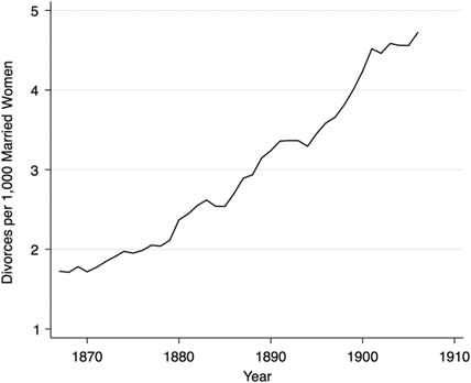
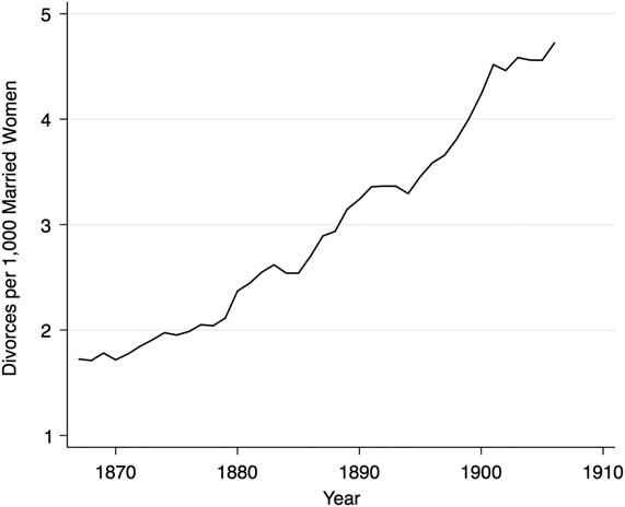
Average divorce rate from 1867 to 1906.
Defining the divorce rate as the number of divorces divided by 1,000 married women, with the number of married women as calculated previously, may have a drawback. Scholars have noted a large amount of marriages that existed without cohabitation, also known as desertions (Cvrcek Reference Cvrcek2011; Kennedy and Ruggles Reference Kennedy and Ruggles2014). These were mentioned in the “Literature Review” section. These cases would not be counted as “married” in our census samples because there would be no spouse present at the time that the census was taken, even though they are not technically a divorce either. Thus, our preferred measure may bias the divorce rate upward, and the crude divorce rate thus offers a more conservative and potentially more accurate measure of the real divorce rate. For evaluating causal effects, this possibility of mismeasurement is not a problem if desertions are not correlated with the passage of an MWPA or EA. While we use our preferred measure of the divorce rate as divorces per 1,000 married women in the analysis in this article, we report alternative results using the crude divorce rate in an appendix.
Together with the 1909 report on divorces (which were similarly complete regarding divorces), we have one consistent measure of the divorce rate for the 1867–1906 period, which is divorces per 1,000 married people for each state and will serve as our main dependent variable. We have this variable for 46 states, so that in total we have 1,820 observations.Footnote 4
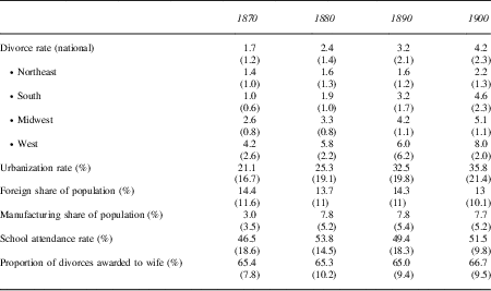
In our analysis, we also control for the age structure of the population, which we define as the percent of the population between 20 and 39 and that can be calculated using the IPUMS microsamples mentioned. Other quantitative data are used later in the article to assess competing explanations for changes in divorce rates in the late nineteenth and early twentieth century: urbanization rates, school attendance rates, percentage of manufacturing employees in the population, and the percentage of the population that is foreign born. These data are taken directly from US Census Reports for the relevant years.Footnote 5 Finally, later in the article we analyze data from the Wright (Reference Wright1889) and Hunt (Reference Hunt1909) reports on the percentage of all divorce proceedings initiated by the wife. Summary statistics for these variables are reported in table 2.
Summary statistics, 1870–1900

Sources: 8th, 9th, 10th, 11th, 12th, and 13 U.S. Censuses.
According to table 2, the average divorce rate for the 1867–1906 period increased from 1.7 in 1870 to 4.2 in 1900. The overall within-state variation was 3.2 and the between-state variation was 2.5, suggesting that factors that occurred to states at certain points of time, like the MWPAs or EAs, contributed more to changes in the divorce rate than state-specific differences that were constant over time. Using standard definitions of regions, starting in 1870 the South had the lowest average divorce rate and the West had the highest, though the South overtook the Northeast by 1890. The western region consistently had the highest amount of overall variation in divorce rates. Urbanization rates increased over time, while the foreign share of the population declined slightly and school attendance rates average around 50 percent.
Figure 2 plots the average divorce rate (the average of our state divorce rates, weighted by married couples) from 1867 to 1906. The divorce rate increased for most of this period, though it did decline slightly in the mid-1880s and 1890s. The fourfold increase in the rate over the entire period provides the major reason why social commentators brought increased attention to marital disruption beginning in the late nineteenth century (e.g., see Smith Reference Smith1884).
Methodology
The empirical strategy used to test the preceding framework is based on a modified version of the difference-in-differences model. Because many states passed their MWPA or EA between 1867 and 1906 in different years, we compare divorce rates in states that did not have an MWPA or EA with states that had one of these laws, or both. Assuming the passage of a property or EA is not itself a function of rising or falling divorce rates, and that some process is not causing both higher divorce rates and the passage of an MWPA or EA, we can infer from our results whether a law caused the divorce rate to increase or decrease relative to those state-years in which an act was not in effect (Angrist and Pischke Reference Angrist and Pischke2009). While the latter of these assumptions might be flawed (i.e., there could have been trends in these states that led to both an MWPA/EA and higher divorce rates), later we introduce two additional approaches to address this issue and support our causal argument.
The baseline approach uses the fact that there were two laws, with each state either enacting a law or not, leading to four possible outcomes (no law, having an MWPA, having an EA, or having both laws). Thus, we construct three dummy variables (with the first case, having no law, serving as the reference group): a variable that equals 1 if a state only had an MWPA (“MWPA only”) and 0 otherwise, another that equals 1 if a state only had an EA (“EA only”) and 0 otherwise, and another that equals 1 if a state had both an EA and an MWPA and 0 otherwise (“Both”). For example, Illinois enacted its MWPA in 1861 and its EA in 1869. Thus, for the years 1861–68, its MWPA dummy variable would equal 1 and equal 0 otherwise. Its EA dummy variable would equal 0 for all years. The “Both” variable would equal 1 starting in 1869, onward, and 0 otherwise. This approach allows us to control for cases in which only one of the laws is present, allowing us to isolate their effect on the divorce rate. It also allows us to see, through the “Both” dummy, whether there were complementary effects of the MWPAs and EAs—because having both laws meant that a married woman was much further away from coverture in terms of her ability to act as an independent economic agent.Footnote 6 From our theoretical framework in the “Literature Review” section, we expect the coefficient for the MWPA dummy variable to be positive and significant, the EA coefficient to be smaller in magnitude than the MWPA coefficient, and the coefficient for the “Both” dummy variable to be positive and significant.
Additional year and state fixed effects are added to control for year-specific changes in the divorce rate common to all states and for state-specific changes common to all years. We also include a control for the age structure of the population (percent of population between 20 and 39) because this is an age group with a higher probability of marriage and divorce, and it is well-known that midwestern and western states generally had higher proportions of people in these age groups. As a first check on our causal argument, we also include region-specific time trends as controls due to the regional variation across time present in the summary statistics of divorce rates in table 2. The following model will therefore be estimated:
 $$\eqalignno{ {\rm Divorce\_rate}_{{{\rm st}}} &{\rm {\, \equals \, }\alpha {\plus}\beta }_{{\rm 1}} \,{\rm {\asterisk}}\,{\rm Property\_Law\_Only}_{{{\rm st}}} {\rm {\plus}\beta }_{{\rm 2}} \,{\rm {\asterisk}}\,{\rm Earnings\_Law\_Only}_{{{\rm st}}} \cr & \quad{\rm {\plus}\beta }_{{\rm 3}} \,{\rm {\asterisk}}\,{\rm Both\_laws}_{{{\rm st}}} {\rm {\plus}} {\rm \delta }_{{\rm 1}} \,{\rm {\asterisk}}\,{\rm Year}_{{\rm t}} {\rm {\plus} \delta }_{{\rm 2}} \,{\rm {\asterisk}}\,{\rm State}_{{\rm s}} {\rm {\plus}\lambda }\,{\rm {\asterisk}}\,{\rm Age\_structure}_{{{\rm st}}} \cr & \quad {\rm {\plus}\tau }\,{\rm {\asterisk}}\,{\rm Region}_{{\rm s}} \,{\rm {\asterisk}}\,{\rm T}_{{\rm t}} {\rm {\plus} {\epsilon}}_{{{\rm st}}} {\rm .} $$
In the preceding model, “Property Law Onlyst” and “Earnings Law Onlyst” are equal to 1 if a state had an MWPA or EA only in year t, while “Both lawsst” is equal to 1 when a state had both laws. The dummy variables “Yeart” and “States” account for cross-year and cross-state differences. The regional trend variable interacts a region dummy with an index variable that goes from 1 to 40 for each state. One region is excluded among the region-specific time trends—the Northeast—so that the trend coefficient vector τ measures regional trends in the divorce rate relative to that region. The estimate of coefficients β1, β2, and β3 represent the main estimates of interest.
In a second specification of our empirical model, we modify the preceding regression equation by replacing the law change variables with leads and lags of these variables. This approach allows us to test whether divorce rates may have already been increasing (or decreasing) prior to the onset of a change in the law, providing a further check on our causal argument. This approach also allows us to assess when we begin to see a marked change divorce rates. The model to be estimated is the following:
 $$\eqalignno{ {\rm Divorce\_rate}_{{{\rm st}}} & {\rm {\, \equals \, } \alpha {\plus}\Sigma }^{{\rm 2}} _{{{\rm \tau {\equals}{\minus}4}}} \,{\rm \beta }_{{{\rm t{\minus}\tau }}} \,{\rm {\asterisk}}\,{\rm Property\_Law\_Only}_{{{\rm st}}} \cr & \quad {\rm {\plus}\beta }_{{{\rm t{\plus}5}\,{\rm foward}}} \,{\rm {\asterisk}}\,{\rm Property\_Law\_Only}_{{{\rm s,t{\plus}5}\,{\rm forward}}} \cr & \quad {\rm {\plus}} {\rm \Sigma }^{{\rm 2}} _{{{\rm \tau {\equals}{\minus}4}}} {\rm \gamma }_{{{\rm t{\minus}\tau }}} \,{\rm {\asterisk}}\,{\rm Earnings\_Law\_Only}_{{{\rm st}}} \cr & \quad {\rm {\plus}\gamma }_{{{\rm t{\plus}5}\,{\rm foward}}} \,{\rm {\asterisk}}\,{\rm Earnings\_Law\_Only}_{{{\rm s,t{\plus}5}\,{\rm forward}}} \cr & \quad {\rm {\plus} \Sigma }^{{\rm 2}} _{{{\rm \tau {\equals}{\minus}4}}} \,\phi _{{{\rm t{\minus}\tau }}} \,{\rm {\asterisk}}\,{\rm Both}_{{{\rm st}}} {\rm {\plus}} \phi _{{{\rm t{\plus}5}\,{\rm foward}}} \,{\rm {\asterisk}}\,{\rm Both}_{{{\rm s,t{\plus}5}\,{\rm forward}}} {\rm {\plus}\delta }_{{\rm 1}} \,{\rm {\asterisk}}\,{\rm Year}_{{\rm t}} \cr & \quad {\rm {\plus}\delta }_{{\rm 2}} \,{\rm {\asterisk}}\,{\rm State}_{{\rm s}} {\rm {\plus}\lambda }\,{\rm {\asterisk}}\,{\rm Age\_structure}_{{{\rm st}}} {\rm {\plus} {\epsilon}}_{{{\rm st}}} {\rm .} $$
“Property Lawt-τ,” “Earnings Lawt-τ,” and “Botht-τ” equal 1 if a law (both laws) is (are) passed in year t-τ (and 0 everywhere else), where τ ranges between -4 and +2, indicating 2 policy leads and 4 policy lags, plus a “5 year and forward” control to account for effects on the divorce rate in all years after the fourth year that the law(s) is (are) passed.
We also empirically assess other potential explanations of the rise in divorce rates during this period that were discussed in the literature review: urbanization, schooling attendance rates (which are one sign of increased economic opportunity), economic development, and foreign immigration. These will be assessed using decennial census data and a first-differenced model regressing the change in divorce rates between 1870 and 1900 on changes in urbanization, schooling attendance rates, the manufacturing share of employment, and the share of foreign immigrants. The model is specified as follows:
 $$\eqalignno{ {\rm \Delta }_{{{\rm st}}} \,{\rm Divorce\_rate} & {{\, \equals\, }\beta }_{{\rm 1}} \,{\rm {\asterisk}}\,{\rm Property\_Law\_Only}_{{{\rm st}}} {\rm {\plus}\beta }_{{\rm 2}} \,{\rm {\asterisk}}\,{\rm Earnings\_Law\_Only}_{{{\rm st}}} \cr & \quad {\rm {\plus}\beta }_{{\rm 3}} \,{\rm {\asterisk}}\,{\rm Both\_laws}_{{{\rm st}}} {\rm {\plus}} {\rm \theta {\asterisk}\Delta }_{{\rm t}} \left[ {{\rm X}_{{{\rm st}}} } \right]{\rm {\plus}{\epsilon}}_{{{\rm st}}} {\rm .} $$
In this model, “Property Law Only,” “Earnings Law Only,” and “Both laws” equal 1 if a state had passed either a property, earning law or both at some point between 1871 and 1880, 1881–90, or 1891–1900, and is equal to 0 otherwise. The variable “Xst” includes the controls for urbanization, schooling, manufacturing, and the foreign share of the population.
Before moving to the results of the analysis, one final point about our empirical strategy concerns the use of population weights. In two studies that are similar to ours, Friedberg (Reference Friedberg1998) and Wolfers (Reference Wolfers2006) examined the impact of unilateral divorce laws on state-level divorce rates (measured as the number of divorces per 1,000 population) in the 1950s through the 1980s using a modified difference-in-differences strategy. Both used weighted least squares (WLS) regression models in which each observation at the state-year level is weighted by state population. In a footnote, Friedberg defends the choice of WLS, rather than ordinary least squares (OLS) regression, by arguing that “a positive effect of [a unilateral divorce law] in, say, California, will carry more weight than a positive effect in New Hampshire” (Friedberg Reference Friedberg1998: 611). Both Friedberg and Wolfers then report WLS standard errors that are not robust to other arbitrary forms of heteroscedasticity.
However, as Lee and Solon (Reference Lee and Solon2011) and later Solon et al. (Reference Solon, Haider and Wooldridge2015) note, divorce rates can be highly correlated within each state (i.e., they are serially autocorrelated), implying that weighting divorce rates by population without any further adjustments to the variance-covariance matrix may make WLS a worse choice than OLS. Instead of WLS, they suggest reporting OLS estimates that are clustered at the state level to account for the correlation in divorce rates within each state.Footnote 7
A second more fundamental point made by Solon et al. (Reference Solon, Haider and Wooldridge2015) is that WLS should not be used to address problems with the underlying model. For example, note that Friedberg’s defense of WLS essentially rests on the idea of heterogeneous treatment effects (i.e., that the law will affect California more than New Hampshire), which can be modeled by including state indicator variables—say, for California and New Hampshire—and interacting those with the yearly indicator for the law, to measure the average effect of the law on the divorce rate in California compared to New Hampshire. Assuming our model is not misspecified in such a way, WLS estimates are not necessary and might even produce biased standard errors if autocorrelation is present and not corrected for. We do not believe that population weights are necessary we choose to err on the safe side regarding standard errors (Angrist and Pischke Reference Angrist and Pischke2009: 91–94).
Analysis—Main Results
In the following subsections, we estimate models 1 through 3; consider the effects of divorce law on the rise in divorce rates; test for alternative explanations for the rise in divorce rates such as urbanization, economic development, and foreign immigration; and finally, examine court cases in which the MWPAs were used to defend a woman’s property from her husband’s claims over it during divorce proceedings.
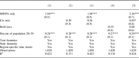
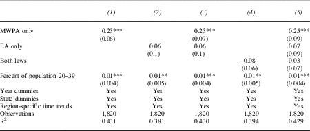
Results from estimating model 1 (with year and state dummies as well as regional time trends) with the 1867–1906 data are presented in table 3. For inference, we use standard errors clustered at the state level to account for serial correlation of divorce rates within each state.Footnote 8 We use the MacDonald (Reference MacDonald2015) dates of passage of the MWPAs and EAs because they correct for judicial interpretation of the legislation originally summarized in Geddes and Tennyson (Reference Geddes and Tennyson2013).Footnote 9
Effects of MWPAs and EAs on divorce rates, 1867–1906

Sources: Wright (Reference Wright1889) and Hunt (Reference Hunt1909) for divorce data; US Censuses (9th, 10th, 11th, 12th, 13th) for data on married women; MacDonald (Reference MacDonald2015) for MWPA and EA dates of passage.
Note: Standard errors corrected for clustering at the state level are in parentheses. Significance measured using critical values from a T-distribution with G-1 degrees of freedom, where G = number of clusters (46). Divorce rate measured as divorces per 1,000 married women, measured using the IPUMS census microsamples (Ruggles et al. Reference Ruggles, Genadek, Goeken, Grover and Sobek2015).
Regional trend coefficients for column 5: Midwest (-0.003), South (0.01), West (0.13***).
*, **, and *** represent significance at the 90%, 95%, and 99% confidence levels, respectively.
The estimates support the hypothesis that the property acts raised divorce rates (coefficient: 2.36). They also show the positive effect of age structure, where state-years with a higher proportion of their population aged 20 to 39 being associated with higher divorce rates, holding all else constant—according to column 5, for example, a 1 percentage point increase in the percentage of the population age 20 to 39 is associated with a 0.29 increase in the divorce rate. Finally, the estimates support the hypothesis that the EAs raised divorce rates, though at a lower rate than the property acts (coefficient: 0.86). This coefficient is also significant only at the 90 percent confidence level (p-value = 0.065) Taken together, the estimates of the effects of the MWPAs and EAs are consistent with the theoretical framework discussed earlier, which predicted that because an increase in the wife’s unearned income raises her fallback utility by a greater amount than an increase in her earned income, the effects on the probability of divorce will be stronger. The regional trends in column 5 are not significant except for the West, which is positive and significant. This finding is consistent with historical research, mentioned in the “Literature Review” section, by Griswold (Reference Griswold1982) that argued that many western states had higher rates of divorce due to the relatively stronger position of women. All regressions in table 3 employ state- and year-fixed effects.
The size of the effect of the property acts is also significant. The (unweighted) mean divorce rate in the sample is about 4.2. Thus, a coefficient of 2.36 in the most complete specification represents more than a 50 percent increase in the average divorce rate in states that had only enacted an MWPA. Also, the estimated coefficients of the trend variables in column 5 suggest that relative to the northeast, divorce rates in the western region were trending upward, while the relative trends in the South and Midwest are not statistically distinguishable from 0. The reason for the rising trend in divorce in the West has been attributed to the migration of younger people to the region—a relationship that is picked up and supported empirically by the coefficient on age structure.
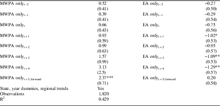
While the significance of the estimates of the property acts and EAs coefficients in column 5 provides substantial evidence that our results are indeed illustrating a causal effect, another way to assess the claim of causality is to include leads and lags of each policy variable to analyze how divorce rates were moving prior to and immediately after the passage of an MWPA or EA. This is the strategy behind model 2. If we find a statistically significant increase in divorce rates prior to the passage of a property act, for example, the causal claim implied by the results in table 3 is weakened.Footnote 10
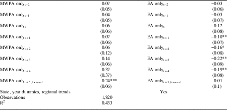
Table 4 shows estimates of model 2 (with leads and lags of each of the law change variables) along with the standard errors. For the property acts, the T-2 and T-1 coefficients (i.e., estimates of the 2- and 1-year policy leads) are positive but are not statistically significant. At T = 0, the year that the property act is passed, the coefficient increases but is still not significant. Only the T = 5+ coefficient is significant (and positive), indicating that the property acts take at least five years until they begin to affect divorce rates. This is logical because, in most cases, the property acts could not be applied retroactively (Basch Reference Basch1979), meaning that only marriages that took place beginning in the year that the law went into effect could be covered by an MWPA.
Dynamic effects of the MWPAs and EAs on divorce rates, 1867–1906

Sources: Wright (Reference Wright1889) and Hunt (Reference Hunt1909) for divorce data; census microsamples from IPUMS (Ruggles et al. Reference Ruggles, Genadek, Goeken, Grover and Sobek2015); MacDonald (Reference MacDonald2015) for MWPA and EA dates of passage.
Note: Standard errors corrected for clustering at the state level are in parentheses.
*, **, and *** represent significance at the 90%, 95%, and 99% confidence levels, respectively.
The coefficients for the EAs are all negative and a few are significant, but neither of the pre-act (T-2 or T-1) coefficients are significant. This finding suggests that the EAs may have played some role in reducing divorce rates by making the marriage more egalitarian. However, over the longer term (T = 5+, or five years and forward), the EAs had no effect on divorce rates in either direction. We thus conclude that while accounting for the dynamics of the laws’ effects does not eliminate the significance of the property acts, it does eliminate the significance of the EAs, supporting our theoretical claim that argued that the property acts will have a stronger impact on divorce rates than the EAs.Footnote 11
To summarize, the results in tables 3 and 4 provide evidence to support the hypothesis that the property laws had a statistically significant effect on divorce rates. Because the coefficient on the EAs variable is statistically significant in table 3, but the long-term coefficient in table 4 is not significant, we argue that the EAs were not effective. Note, however, that our theoretical framework predicted that the effects of an increase in unearned income on the wife’s fallback option (i.e., utility after divorce) will have a stronger effect on the probability of divorce than the effects of increased earned income. Thus, our findings are consistent with the external threat model of household bargaining. We also note at this point that married women’s labor force participation was low, diminishing the impact of any earnings law. In addition, MacDonald (Reference MacDonald2015) found that even if a wife acquired earnings from market work, judges sometimes found ways of ruling that these earnings were still the property of the husband—especially if the work that was performed was argued to be connected to the wife’s marital obligations to her husband and family (on this point, see Siegel Reference Siegel1995).
Effects of Divorce Law
One hypothesis for the rise in divorce rates in the late nineteenth century is that there may have been liberalizations in state divorce law, especially because forces driving changes in divorce law—such as women’s movements or attitudinal changes toward the family—could have led to the passage of MWPAs and EAs as well. However, there are some reasons to doubt this claim. First, Amato and Irving (Reference Amato and Irving2006) argue that increased demands for divorce are what changed divorce law, not the other way around. Second, many scholars have argued that divorce law did not have a major impact and instead attribute divorce to economic, ideological, or attitudinal factors (Ruggles Reference Ruggles1997; Schultz Reference Schultz1984, Reference Schultz1986, Reference Schultz1990—see the “Literature Review” section for more discussion of these factors). In the earlier part of the nineteenth century, for example, omnibus clauses were enacted in some states, and Schultz (Reference Schultz1984) argued that these could explain the high rate of divorce in Illinois. However, the omnibus clause in Illinois was enacted in 1833 and would therefore be picked up by our state-level fixed effects. Indiana also had an omnibus clause in 1825 and would be accounted for as well. The presence of an omnibus clause in Illinois also fails to explain why divorce rates in other midwestern states such as Indiana, Iowa, and Michigan increased at roughly the same rate, if not more than Illinois, between 1867 and 1906.Footnote 12
Regarding divorce law, Schultz concluded for the earlier part of the nineteenth century that “any relationship between divorce grounds and divorce rates was more closely tied to the nature, rather than the number, of legal grounds” (Schultz Reference Schultz1984: 519). Indeed, there were a core of six grounds that constitute about 97 percent of all divorces in the 1867–86 sample, according to Willcox (Reference Willcox1897): desertion, adultery, cruelty, drunkenness, neglect to provide, imprisonment, or some combination of all these. But on this point, a state’s failure to cover all six of these grounds did not necessarily mean it would have a low divorce rate: New York only allowed for adultery, but it had a higher rate than Pennsylvania, which had adultery as well as three more of the major grounds (Willcox Reference Willcox1897: 45).Footnote 13
Even when states added new causes, such as when Alabama added drunkenness in 1870, there was no increase in divorce rates, not even an increase in divorces for that particular reason. Furthermore, considering that Alabama never had a MWPA and only had an EA after 1887, there was little relation between these laws and the divorce law for drunkenness. In other cases, sharp increases in the number of divorces and the divorce rate in states such as Florida around 1900, Arkansas between 1880 and 1890 and after 1900 (indeed, in much of the South, as our summary statistics show), and in Ohio throughout, all occurred without any major change in the state’s legislation. Thus, the laws did not have any effect on divorce rates in many cases.
A final point regarding divorce law is that, due to the stark increase in divorces in the late nineteenth century, “the whole trend of both legislation and administration has been toward greater stringency” (Lichtenberger Reference Lichtenberger1909), meaning that divorce rates increased despite restrictive legislation—and the restrictive legislation, in turn, was happening at the same time as the liberalization of married women’s property rights. For example, omnibus clauses were not used by states later in the nineteenth century, as many states moved to stricter requirements for divorce as a direct response to the rise in divorce rates. This point was also made by historians of divorce for this period, such as in O’Neill (Reference O’Neill1965) and Halem (Reference Halem1980), both of whom focused on divorce law and found that while the law was attempting to reduce the social strain caused by the increase in divorces, these efforts were largely in vain.
Thus, we conclude that because MWPAs and EAs were moving in one direction—toward greater liberalization of women’s position in the household—while divorce law was moving in an opposite direction—toward stricter laws governing women’s ability to divorce—the two sets of laws were independent of each other and possibly even moving against each other. While there were some changes in divorce process, especially around the 1880s, including provisions for notice to the defendant and defending the suit, these are not enough to explain a wide-sweeping increase in divorce rates during this time (Lichtenberger Reference Lichtenberger1909).
Effects of Urbanization, Economic Development, and Foreign Immigration
We consider alternative explanations for the rise in the divorce rates in the late nineteenth century. The historical studies mentioned in the “Literature Review” section highlighted urbanization (due to the increased influence of norms of independence and improved labor market opportunities), foreign immigration (such as the influx of Catholics who had a stricter view of divorce), and economic development (which could increase or decrease marital stability by increasing economic opportunities for married women). Because these factors have been the major ones cited in the literature, we use pooled data from the 1870–1900 censuses and regress changes in the state-level divorce rate between 1870–80, 1880–90, and 1890–1900 on changes in the urbanization rate, share of the state’s population that is foreign born, share of manufacturing workers in the population, and the schooling attendance rate. Based on previous literature and holding constant the other factors, the urbanization rate is expected to increase divorce rates; the increase in foreign population is expected to decrease divorce rates; the share of manufacturing workers is expected to increase divorce rates; and the schooling rate is expected to have increased divorce rates due to the increased returns to women’s labor (and thus the labor market) provided by the increase in education (Geddes and Lueck Reference Geddes and Lueck2002; Geddes et al. Reference Geddes, Lueck and Tennyson2012).
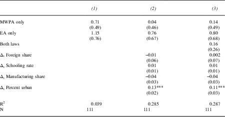
Column 3 of table 5 presents the main estimates. After accounting for other factors, changes in urbanization are positively related to changes in the divorce rate. However, the rest of the coefficients—for the change in the foreign share of the population, share of manufacturing workers, and schooling attendance rate—are not significant. The law coefficients are not significant, but because of the framework used in this section (where we use decennial data) they are imperfectly specified and are thus not reliable estimates of the laws’ relationship with divorce rates. The major result from this section is that while urbanization is supported as a cause of divorce, other explanations provided in the literature such as economic development or foreign immigration are not supported as a cause. Note, however, that urbanization brings with it changes in economic opportunities for women and general cultural changes such as individualism that are mechanisms whereby the divorce rate can increase. Also, in the “Analysis—Main Results” section we found that age structure positively affected divorce rates, which was another factor identified in the literature (such as in Griswold Reference Griswold1982).
Effects of economic variables on divorce rates, 1870–1900 (dependent variable: Δt[Divorce_ratest])

Sources: 9th, 10th, 11th, and 12th US Censuses for nativity, schooling, manufacturing, and urbanization statistics.
Note: Robust standard errors in parentheses.
*, **, and *** indicate significance at the 90%, 95%, and 99% confidence levels, respectively.
Court Case Analysis
Another way to assess the relationship between married women’s property law and the increase in late-nineteenth-century divorce rates is to consider the intersection of these two areas in court cases. According to the excerpt from Shammas (Reference Shammas1994), due to the MWPAs and EAs, married women had less to lose from separating from their husbands, and this should have made divorce more likely. Did the MWPAs ensure that the wife could recover her property after separation? While it seems likely, it is also possible that courts found ways of arguing that the property really did not belong to her.
We first consider data from Wright (Reference Wright1889) and Hunt (Reference Hunt1909) on the percentage of all divorces in each state awarded to the wife to analyze whether the MWPAs and EAs were in part responsible for this trend. We know that women were increasingly more likely to petition for divorce—by 1909, 67.5 percent of all divorces were initiated by the wife (Lichtenberger Reference Lichtenberger1909), up from 61.5 percent in 1867. While these data omit cases in which the wife (or husband) filed for a divorce and were unsuccessful, any unobserved judicial bias would likely bring the effects downward because it is likely that women were less successful than men in obtaining a divorce, so that our estimates likely underestimate the effects of the MWPAs and EAs.
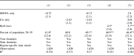
The proportion of successful petitions initiated by the wife did vary by legal environment, but not always in the expected way: States with both an MWPA and EA had 67.3 percent of divorces awarded to the wife, compared to 60 percent for states that had neither an MWPA or EA. States with just an MWPA had 62.6 percent of divorces awarded to the wife (vs. 64.5 percent without an MWPA), while states with just an EA only had 51 percent (vs. 64 percent without an EA). These differences are statistically significant, but they suggest that having a law might have lowered the fraction of petitions awarded to the wife. The “both” category suggests the opposite, but this could simply be picking up the fact that that, over time, states increasingly had both laws on their books. The results in table 6 show that after accounting for state and year fixed effects in a regression model of divorce petitions awarded to the wife on the law change variables, there is a statistically significant effect of having both laws (see column 5), meaning that having a legal environment that was progressively closer to removing the restrictions of coverture did increase the ability of women to petition for (and achieve) divorce.
Effects of MWPAs and EAs on percentage of divorces awarded to wife

Sources: Wright (Reference Wright1889) and Hunt (Reference Hunt1909) for divorce data; MacDonald (Reference MacDonald2015) for MWPA and EA dates of passage.
Note: Standard errors corrected for clustering at the state level are in parentheses. Significance measured using critical values from a T-distribution with G-1 degrees of freedom, where G = number of clusters (46).
*, **, and *** represent significance at the 90%, 95%, and 99% confidence levels, respectively.
To explore further whether the property and EAs mattered substantively in divorce proceedings, we searched a well-known legal database, WestLaw, for state-level cases involving divorce and claims to property made by the wife against her husband.Footnote 14 We were looking for two main scenarios: (1) Court case briefs may have referenced an MWPA during divorce proceedings but then the justice may have ultimately ruled on some other grounds. (2) The justice might have ruled an MWPA irrelevant to a wife’s claim to property because of the lack of retroactive application of the statute or the general conservatism of the judiciary during this time (Basch Reference Basch1979; MacDonald Reference MacDonald2015). Case analysis will shed light on how the MWPAs operated in divorce proceedings.
To conduct a general search, we initially searched state law reporters published in WestLaw for the strings “wife,” “property,” and “divorce,” and then “wife,” “earnings,” and “divorce,” between 1860 and 1900. We found about 4,000 cases using these search terms (mostly involving property, with only about 300 involving earnings), but as we searched through them, many did not reference a state’s MWPA or EA and even fewer were about both an MWPA or EA as well as a former wife’s rights to property or earnings after marriage—either ruling for her ownership rights or against them. For the few relevant cases, we used WestLaw’s “Citing References” option to find cases that cited these cases (as well as in-text citations to previous cases that we may have missed in our initial search), leading to a larger sample. In the end, we analyzed about 35 cases, and we summarize our findings from five that are representative of the others.
One of the more common disputes arose when a married woman lent her husband money based on her personal property and then sued for that property after divorce. Under coverture, such a contract was considered null and void: A wife’s property was owned exclusively by the husband and she was also assumed to be non compos mentis, or not of a sound mind to enter independently into contracts. After the MWPAs, contracts in which the wife sold some of her property to her husband in exchange for a promissory note were more often, though not always, ruled as lawful, and at any point after the dissolution of the marriage contract, the wife could maintain an action in court (typically an action of assumpsit, i.e., on a breach of contract) on the note if her former husband refused to pay.
A case was heard at the Supreme Judicial Court of Maine in 1870 in which Miranda Webster sued James Webster, her former husband, on the claim for a promissory note given to her during marriage. The note was signed and dated January 22, 1861 for the sum of 50 dollars plus interest. Maine’s property act was passed in 1855 and thus the contract fell within the ambit of the statute. The divorce was made official in October 1869, after which the suit took place. The initial ruling was made in the Cumberland County court in favor of Miranda Webster, but James Webster alleged exceptions, at which point the state’s Supreme Court heard the case (Webster v. Webster, 58 Me. 139, 140, 141, 143, 1870).
Chief Justice John Appleton began his opinion by noting that “[b]y common law, marriage is an absolute gift to the husband of all the goods, personal chattels, and other personal state, of which the wife is actually or beneficially seized at the time in her own right…. But the statutes of this state have made great and important innovations upon the rules of the common law” (Webster v. Webster, 1870: 140–41). Appleton acknowledged the relevance of the state’s property act. Responding to the husband’s claim that the promissory note was void (because of the existence of a marital contract between them that prevented conveyances of property), Appleton observed that “the note of the husband to the wife is not void. To declare it so, or the loan, of which it is evidence, would be to fail in giving the wife the protection which the statutes [i.e., the MWPA] were intended to afford” (Webster v. Webster, 1870: 143). Appleton overruled the exceptions initially brought forward by the husband, affirming the wife’s property right in the money promised. Also noteworthy is that the other justices at the court (Kent, Walton, Barrows, Danforth, and Tapley) were all reported as concurring with Appleton’s opinion.
In his recorded opinion, Appleton responded to some of the claims made by the defense about the validity of the promissory note. For example, the husband’s defense in the Webster case rested on two arguments: first, that the husband and wife “are not competent parties to a contract” and, second, that “[t]he contract, or note, in this suit is void, and cannot be enforced in law.” The first point is countered by the MWPA, which (for Appleton) is power enough to even override the claim of non compos mentis (a claim made against women who were argued to not be “of sound mind” to enter into a contract). This is a strong ruling, though it was also influential: It was later used in a Kansas case (Going v. Arns, 8 Kan. 85, 1871) in which the wife, who used her separate property to purchase a horse from her husband, could claim ownership after her husband had tried to sell the horse to pay off his debts. Appleton’s opinion in Webster was used to defend the ability of the married woman to enter such contracts.
The second argument—that the suit is void—is countered by numerous precedents from other states ruling that such contracts were valid. Appleton cited cases from Rhode Island, Iowa, Ohio, and Pennsylvania, all in favor of the wife’s property rights. Most of these cases did not refer specifically to the issue of a divorced woman seeking payment on a promissory note or other contract. They were used to substantiate Miranda Webster’s claim of a property right separate from that of the husband.Footnote 15
At any rate, these cases show the usefulness of the acts for married women. Prior to the acts, this contract would have held little meaning in the eyes of the common law, and it would have been more difficult for the woman to separate. With the passage of the acts, however, particularly those awarding ownership and control rights, women could be assured of these sources of property after the dissolution of the marriage. They would not lose as much from a divorce and thus the wife’s bargaining power would increase, raising the probability of a divorce.
Further proof of the importance of these acts for married women stems from the fact that when a property act was not in force, the wife often could not maintain an action of assumpsit on a promissory note. In other words, wives had trouble obtaining claims to their property before the MWPAs. In Patterson v. Patterson (45 N.H. 164, 166, 1863), the husband issued a promissory note on property that he received from his wife. While the case is from 1863 (placing it after the date of New Hampshire’s MWPA of 1860), the actual contract was signed in 1844 and thus fell outside of the ambit of the law. The promissory note was for $1,536.96. Justice Bellows gave the opinion in the court. The opinion relied on the common law of coverture, which was valid precisely because of the lack of any MWPA: Bellows noted toward the end of his opinion, “Nor do we perceive that the case is brought within any of the provisions of our statutes which give a married woman power to contract as sole. It does not appear that the property for which the original note was given was held by the wife to her sole and separate use; or that the case comes within any of the provisions which authorize her to act as if sole” (Patterson v. Patterson 1863: 166).Footnote 16 Thus, the courts recognized that the lack of a MWPA posed a real barrier to a wife’s ability to make claims on property that she conveyed.
Conclusion
This article has used a household bargaining framework to analyze whether a significant change in married women’s property rights influenced divorce rates in the late-nineteenth- and early-twentieth-century United States. Given how momentous the laws were, and their coincidence with industrialization as well as women’s movements, there is good reason to argue that the laws may have also made it easier for wives to obtain a divorce. In the household bargaining literature, an increase in unearned income raises the threat utility (utility outside of the marriage) and can thus increase the probability of divorce. We found evidence to support this framework: The MWPAs increased divorce rates in those states that passed them relative to those that did not. We also found that the EAs did not have a long-term effect, after controlling for the timing of the passage of these laws.
We provided additional support for our causal claims: Divorce rates were not already increasing prior to an MWPA or EA, the liberalization of divorce law was not the cause of higher divorce rates (if anything, law worked against the rise in rates), and we found several examples of court cases in which a woman used the MWPA to secure her property against the claims of her ex-husband, which provided further proof of the operational use of the laws in divorce proceedings and indirect evidence of the extent to which they raised married women’s bargaining power.
Our research contributes to the history of divorce in the late nineteenth century as well as a growing body of literature documenting the economic and social implications of self-ownership for married women. Women’s economic independence played a crucial role in altering household dynamics in the nineteenth- and early-twentieth-century United States