
I. INTRODUCTION
Nanoindentation, also known as instrumented or depth-sensing indentation, has become a widely accepted materials characterization technique, and international standards for instrumented indentation testing have been elaborated since 2007. 1 During nanoindentation tests, a small indenter tip is pressed into the sample and both the applied load and the displacement of the material are measured, allowing its mechanical properties such as reduced modulus and hardness to be calculated. Although traditional nanoindentation techniques were developed for stiff materials, such as metals and ceramics, nanoindentation testing of compliant materials, such as soft tissues, cells, and hydrogels, has recently attracted substantial attention because the high spatial resolution of nanoindentation allows local testing of mechanical properties of soft matter that is not possible using macroscale techniques. Reference Ebenstein and Pruitt2–Reference Klapperich, Pruitt and Komvopoulos25 For example, Ferguson et al. applied the nanoindentation technique to human articular calcified cartilage and subchondral bone from normal and osteoarthritic patients Reference Ferguson, Bushby and Boyde21 ; Leong and Morgan used the same technique to describe local changes in the mineralization across a rat fracture callus Reference Leong and Morgan22 ; and the surface mechanical properties and deformation behavior of ultrahigh molecular weight polyethylene were examined by nanoindentation experiments performed with a surface force microscope. Reference Klapperich, Pruitt and Komvopoulos25 However, nanoindentation is not readily applicable to softer materials yet, as numerous challenges remain to be overcome.
One of the key concerns associated with nanoindentation testing of soft materials is the significant effect of adhesion between the indenter tip and the sample. Adhesion leads to larger contact areas and higher contact stiffness for a given applied force relative to the Hertz model, Reference Johnson26 which results in an overestimation of modulus values if the experimental data is analyzed by the traditional Oliver–Pharr analysis method implemented by most commercial software packages, which assumes an elastic–plastic response with negligible adhesion. Reference Oliver and Pharr27 These errors can be significant when testing compliant materials at low indentation depths, such as the range of 60%–300% error in modulus values reported in studies of silicone samples. Reference Gupta, Carrillo, Li, Pruitt and Puttlitz10,Reference Ebenstein23 Moreover, adhesion also makes it quite challenging to determine the initial point of contact of the indenter tip, based on which the contact area and the elastic modulus are calculated. Reference Wang, Volinsky and Gallant16 For soft materials, because of the adhesion of the sample surface, the indenter tip is attracted to it, resulting in a negative load at the beginning of the indentation process, i.e., the so-called pull-in force. As a result, the initial contact point used for calculating the contact area and the reduced modulus in the commercial software is shifted. The reduced modulus values automatically calculated by the software are thus not accurate. Some nanoindentation studies utilized an automated surface approach and ignored this initial contact adhesion force effect, reporting only the positive load portion of the load–displacement curve, which leads to inaccurate estimation of modulus and hardness values. Reference Carrillo, Gupta, Balooch, Marshall, Marshall, Pruitt and Puttlitz8,Reference Alisafaei, Han and Sanei24
Despite the significant errors in modulus values, most studies of soft materials still ignore the effects of adhesion. Only several pioneering studies Reference Carrillo, Gupta, Balooch, Marshall, Marshall, Pruitt and Puttlitz8–Reference Gupta, Carrillo, Li, Pruitt and Puttlitz10,Reference Cao, Yang and Soboyejoy13,Reference Ebenstein23 have sought to extract accurate modulus values from nanoindentation data by methods based on the Johnson–Kendall–Roberts (JKR) model. Reference Johnson26 Unlike the Oliver–Pharr method, the JKR methods seek to fit indentation data with models that take the effect of adhesion into account. These studies have used the force curve approach, where the indenter tip both begins and ends above the sample surface to capture the whole process of loading and unloading as the indenter tip approaches the sample surface, jumps into contact, indents, withdraws, and pulls off from the sample. Experimental measurements are then analyzed by using only two points on the load–displacement curve to calculate the reduced modulus, Reference Ebenstein and Wahl9,Reference Grunlan, Xinyun, Rowenhorst and Gerberich14 or by using direct curve-fitting approaches that also identify the point of initial contact. Reference Ebenstein and Wahl9,Reference Cao, Yang and Soboyejoy13 This technique of combining force curve data collection with the JKR model is often referred to as the nano-JKR force curve method. Reference Ebenstein23 Using the connection between nanoindentation by spherical indenters and mechanics of adhesive contact, Borodich and Galanov then introduced another method, now called the BG method, that is not based on measurement of just one or several values of the experimental load–displacement curves but based on an inverse analysis of all experimental points at a bounded interval of the load–displacement curve obtained for a spherical indenter. Reference Borodich and Galanov28 The BG method is not direct because, instead of direct measurement of the pull-off force, it needs some scaling parameters, and then the pull-off force is calculated using these parameters. Although those approaches have demonstrated their capabilities to correct for errors due to adhesion, Reference Gupta, Carrillo, Li, Pruitt and Puttlitz10,Reference Ebenstein23,Reference Borodich and Galanov28 to our knowledge, they have not been widely adopted, mainly because they work only with perfectly spherical tips and have not been implemented in commercial software.
In this paper, we extend the nano-JKR force curve method to include Berkovich Reference Berkovich29 indenters and flat indenters by conducting a numerical simulation in which the adhesive interactions are represented by an interaction potential and the surface deformations are coupled by using half-space Green’s functions discretized on the surface. In particular, two types of flat indenters are discussed, the cylindrical flat tip and the conical frustum tip. The relationship among the force, the displacement, and the contact area are studied in detail, as these relationships are crucial for the calculation of mechanical properties based on the indentation data. Moreover, the simulations obtain quantities that cannot be easily measured in experiments, such as deformations under the indenter and pressure distribution in contact area, and offer the possibility of varying the indentation conditions in a systematic and controlled way, so that the influences of, for example, adhesion and adhesion hysteresis on the contact area can be studied. The numerical results are also compared with experimental data.
II. MODELS IN CONTACT MECHANICS
Indentation theory is based on contact mechanics, where some well-known models have been derived for simple geometries. Hertz in 1882 published his famous pioneering work on the contact of elastic frictionless bodies, Reference Johnson26 which has become the corner stone in the field of contact mechanics. Hertz based his model on linear elasticity and assumed that the surface adjacent to the point of contact is rounded and may be considered as a surface of second degree. The classical Hertz model is widely implemented today in the design of gears, bearings, rails, and wheels and other machinery parts. This model, however, neglects adhesive forces which become increasingly important for microstructures and nanostructures.
Sneddon Reference Sneddon30 considered a punch of arbitrary profile in contact with an elastic half space and derived a relation between force and penetration depth, as well as for the pressure distribution beneath the indenter and the shape of the deformed surface. These equations of Sneddon now form the basis of the well-known Oliver–Pharr analysis method, Reference Oliver and Pharr27 which is commonly used for evaluating nanoindentation data. Although this method is generally accepted to provide accurate and reliable values of mechanical properties, it is important to note that adhesion is assumed to play a negligible role in the sample deformation.
A first attempt to analyze deformable adhesive contact was made by Johnson, Kendall, and Roberts, Reference Johnson26 who proposed the JKR model, assuming that, as two spheres approach each other and start to form a contact, the initial pressure distribution between them consists of repulsion close to the center and attraction at the edge of the contact area. Different from the JKR model, Derjaguin, Muller, and Toporov Reference Johnson26 proposed the DMT model, which assumes that all the attraction forces act outside the contact area and these forces are too weak to produce any substantial deformations of the spheres. They used the Hertz model to obtain the local gap distribution between the spheres’ surfaces outside the contact area to calculate the total adhesive force.
The discrepancy between these two models was resolved in 1976 by the realization that they are both valid, but in completely opposite limits of contact behavior. Reference Tabor31 When the induced elastic deformations in the materials are large compared with the range of the attractive forces, which occurs for compliant materials, large sphere radii and strong, short-range adhesion forces, the JKR model is accurate. The DMT model is accurate in the opposite limit, i.e., stiff materials, small sphere radii and weak, long-range adhesion forces. These limits are described quantitatively by a dimensionless parameter, which is now referred to as the Tabor parameter, Reference Tabor31 interpreted as the ratio between the normal elastic deformation caused solely by adhesion, not by the applied load, and the spatial range of the adhesion forces. Some recently developed models for the JKR-DMT transition have been summarized in a comprehensive review by Barthel. Reference Barthel32
The first numerical simulation for the adhesive contact between spheres was presented by Muller et al. in 1980, Reference Muller, Yushchenko and Derjaguin33 who used the Lennard-Jones potential to model surface interaction and showed a continuous transition from the JKR to the DMT theory as the Tabor parameter decreased. A complete numerical solution was obtained by Greenwood, Reference Greenwood34 who pointed out the existence of singular integrands in the governing equation and found S-shaped load-approach curves for values of Tabor parameter greater than one, leading to jumps into and out of contact.
All the above-mentioned research focuses on the contact problems between two spheres or between a sphere and a half space. To our knowledge, only a few studies have been focusing on the JKR-type adhesive contact involving more general shapes. An extension of the JKR adhesive frictionless contact problem to monomial punches was first obtained by Galanov in 1993. Reference Galanov35 In the same year, Borodich provided another derivation of Galanov’s solution; however, it was published much later. Reference Borodich and Gladwell36 Some recent results related to the generalization of JKR theory for axisymmetric adhesive contact problems have been reviewed by Borodich. Reference Borodich37
For the contact problems involving non-axisymmetric shapes, the absence of radial symmetry presents significant difficulty in the numerical simulation, because the number of nonlinear equations increases from N to N 2, as discussed Sec. III. In this paper, we use a numerical simulation method in which the adhesive interactions are represented by the Lennard-Jones potential and the surface deformations are coupled by using half-space Green’s functions discretized on the surface. To solve this system of N 2 highly nonlinear equations, a virtual state relaxation (VSR) method has been implemented. Reference Jin, Jagota and Hui38
Finite element modeling for nanoindentation using various indenter geometries has been attempted, with varying levels of accuracy, such as the works of Giannakopoulos et al. Reference Giannakopoulos, Larsson and Vestregaard39 for the analysis of Vickers indentation, Larsson et al. Reference Larsson, Giannakopoulos, Soderlund, Rowcliffe and Vestergaard40 for the analysis of Berkovich indentation, and Chudoba and Jennett Reference Chudoba and Jennett41 for the analysis of conical indentation, but those simulations do not include the effect of adhesion. If the finite element method is used to solve JKR-type adhesive contact problems, a 3D model should be built with a large number of cohesive elements applied at the interface. The semianalytical approach adopted in this paper converts a 3D problem to a 2D problem, and so the computational cost is significantly reduced. In our simulation, the number of meshes at the contact surface is set to be 512 × 512, which will be computationally prohibitive for commercial finite element software.
III. NUMERICAL SIMULATION
In this section, the governing equations of frictionless adhesive contact problems involving general shapes will be presented. For surface atomic interaction, the empirical potential we used is the Lennard-Jones potential. Reference Israelachvili42 Hence, we can obtain the relationship between the local pressure p and the air gap h as follows:
 $$p(h) = {{8{W_{{\rm{ad}}}}} \over {3\varepsilon }}\left[ {{{\left( {{\varepsilon \mathord{\left/ {\vphantom {\varepsilon h}} \right. \kern-\nulldelimiterspace} h}} \right)}^9} - {{\left( {{\varepsilon \mathord{\left/ {\vphantom {\varepsilon h}} \right. \kern-\nulldelimiterspace} h}} \right)}^3}} \right]\quad ,$$
where W ad is the work of adhesion, the tensile force integrated over the distance necessary to pull apart the two bodies, and ε is a length parameter equal to the range of the surface interaction. For stiff materials, the value of ε should be on the order of interatomic spacing; however, for compliant materials its value usually becomes much larger. Reference Hui, Jagota, Bennison and Londono43,Reference Tang, Hui, Jagota and Chaudhury44 Equation (1) was first introduced by Johnson and Greenwood without proof Reference Johnson and Greenwood45 and has since been used in many adhesion studies. Reference Kogut and Etsion46–Reference Song and Komvopoulos48 A detailed derivation of Eq. (1) is provided by Jagota and Argento Reference Jagota and Argento49 and Yu and Polycarpou. Reference Yu and Polycarpou50 Note that the first term in Eq. (1) corresponds to attraction between the surfaces, while the second term corresponds to repulsion. When the local separation is smaller than the interatomic distance, the short-range repulsive forces prevail over the attraction forces and the local traction becomes negative. Otherwise, when the local separation is larger than the interatomic distance, the local traction is positive.
Derjaguin’s approximation Reference Greenwood34 is then applied to Eq. (1). This approximation relates the force law between two curved surfaces to the interaction energy per unit area between two planar surfaces. This approximation becomes a very useful tool, since forces between two planar bodies are often much easier to calculate. The separation between the two surfaces due to the surface interaction as well as the applied load, denoted by h, will be expressed by the following equation Reference Greenwood34 :
 $$h\left( {x,y} \right) = - \alpha + \varepsilon + {h_0} + {1 \over {\pi {E^{{\rm{TI}}}}}}\int\!\!\!\int_\Omega {{{p\left( {x',y'} \right)\,{\rm{d}}x'\,{\rm{d}}y'} \over {{{\left( {x - x'} \right)}^2} + {{\left( {y - y'} \right)}^2}}}} \quad ,$$
where the parameter α is the displacement between the two surfaces with respect to the zero force position h = ε, i.e., the so-called indentation depth, and the parameter E
TI represents the effective elastic contact modulus. Note that E
TI has different expressions for different materials. For the adhesive contact between two linearly elastic isotropic materials with Young’s modulus E
i and Poisson’s ratio ν
i
, where i = 1, 2, E
TI can be approximately described by
 ${E^ * }$
, which is defined as the reduced modulus, also termed the effective modulus:
 $${1 \over {{E^ * }}} = {{1 - \nu _1^2} \over {{E_1}}} + {{1 - \nu _2^2} \over {{E_2}}}\quad .$$
For the adhesive contact between a rigid indenter and a transversely isotropic material, E TI is more complicated and can be written as the following equation Reference Borodich, Galanov, Keer and Suarez-Alvarez51 :
 $${E^{{\rm{TI}}}} = - {{{2{D^{{1 \mathord{\left/ {\vphantom {1 2}} \right. \kern-\nulldelimiterspace} 2}}\left( {AC - D} \right)}}} \over {\left( {{S_1} + {S_2}} \right)\left[ {\left( {D - 2BD + AC} \right){a_{11}} - \left( {2D - BD - AC} \right){a_{12}}} \right]}}$$
with
 $$\!\!\!\!\!\!\!\!\!\eqalignb{ & \;\;A = {{{a_{13}}({a_{11}} - {a_{12}})} \over {{a_{11}}{a_{33}} - \mathop {{a_{{\rm{13}}}}}\nolimits^2 }},\;B = {{{a_{13}}({a_{13}} + {a_{44}}) - {a_{12}}{a_{33}}} \over {{a_{11}}{a_{33}} - \mathop {{a_{{\rm{13}}}}}\nolimits^2 }},\cr\;C = {{{a_{13}}({a_{11}} - {a_{22}}) + {a_{11}}{a_{44}}} \over {{a_{11}}{a_{33}} - \mathop {{a_{{\rm{13}}}}}\nolimits^2 }},\;D = {{\mathop {{a_{{\rm{11}}}}}\nolimits^2 - \mathop {{a_{{\rm{12}}}}}\nolimits^2 } \over {{a_{11}}{a_{33}} - \mathop {{a_{{\rm{13}}}}}\nolimits^2 }} \cr\;\;{S_{1,2}} = \sqrt {{{A + C} \over {2D}} \pm {{\left[ {{{\left( {{{A + C} \over {2D}}} \right)}^2} - {1 \over D}} \right]}^{{1 \mathord{\left/ {\vphantom {1 2}} \right. \kern-\nulldelimiterspace} 2}}}\quad ,} \cr}$$
where a 11, a 12, a 13, a 33, and a 44 are the five elastic constants for the transversely isotropic material. Assume that the z-axis is normal to the plane of isotropy, and then Hooke’s law can be written as follows:
 $$\left( \matrix{ {\varepsilon _{11}} \hfill \cr {\varepsilon _{22}} \hfill \cr {\varepsilon _{33}} \hfill \cr {\varepsilon _{12}} \hfill \cr {\varepsilon _{13}} \hfill \cr {\varepsilon _{23}} \hfill \cr} \right) = \left[ {\matrix{ {{a_{11}}} & {{a_{12}}} & {{a_{13}}} & 0 & 0 & 0 \cr {{a_{12}}} & {{a_{11}}} & {{a_{13}}} & 0 & 0 & 0 \cr {{a_{13}}} & {{a_{13}}} & {{a_{13}}} & 0 & 0 & 0 \cr 0 & 0 & 0 & {{a_{11}} - {a_{12}}} & 0 & 0 \cr 0 & 0 & 0 & 0 & {{{{a_{44}}} \mathord{\left/ {\vphantom {{{a_{44}}} 2}} \right. \kern-\nulldelimiterspace} 2}} & 0 \cr 0 & 0 & 0 & 0 & 0 & {{{{a_{44}}} \mathord{\left/ {\vphantom {{{a_{44}}} 2}} \right. \kern-\nulldelimiterspace} 2}} \cr} } \right]\left( \matrix{ {\sigma _{11}} \hfill \cr {\sigma _{22}} \hfill \cr {\sigma _{33}} \hfill \cr {\sigma _{12}} \hfill \cr {\sigma _{13}} \hfill \cr {\sigma _{23}} \hfill \cr} \right)\quad .$$
Note that the formulae for numerical simulation for the adhesive contact for transversely isotropic materials have the same mathematical form as the corresponding formulae for isotropic materials, except that the effective elastic contact modulus E TI has different expression.
The parameter h 0 in Eq. (2) is the initial air gap written in rectangular coordinates, i.e., the separation of the two surfaces in the absence of applied and adhesive forces. The expression of h 0 is different for different types of indenters:
-
(i) Spherical indenters. In the JKR model, the geometry of a spherical contact is approximated by a parabolic function Reference Greenwood34 :
 $${h_0}(x,y) = {{{x^2} + {y^2}} \over {2R}}\quad ,$$
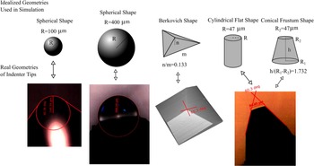
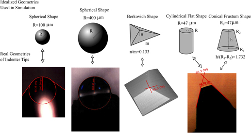
where R is the radius of the sphere indenter, as shown in Fig. 1.
-
(ii) Berkovich indenters. The geometry of a Berkovich tip is a pyramid having a triangular base, as shown in Fig. 1. The initial air gap for a pyramid with a base of an equilateral triangle with side length m and a height of n can be written as follows:
 $${h_0}(x,y) = \left\{ \matrix{ {n \over m}\left( {\sqrt 3 y + 3|x|} \right)\quad {\rm{if}}\;\;|x| > - \sqrt 3 y \hfill \cr {{2\sqrt 3 n|y|} \over m}\quad {\rm{otherwise}} \hfill \cr} \right.\quad ,$$
The idealized geometries of indenter tips used in the numerical simulations and the corresponding real tips used in the experiments, respectively.

For a Berkovich tip, the angle between the centerline and the three faces is 65.3°, which gives n/m = 0.133.
-
(iii) Cylindrical flat indenters. In this case, the initial air gap is zero for points (x, y) inside the circular region x 2 + y 2 ≤ R 2, where R is the radius of the cylindrical flat punch, as shown in Fig. 1.
-
(iv) Conical frustum indenters. A conical frustum is a frustum created by slicing the top off a cone with the cut made parallel to the base. For a right circular cone, let h be the height and R 1 and R 2 the base and top radii, as shown in Fig. 1. Then the initial air gap is zero for points (x, y) inside the circular region x 2 + y 2 ≤ R 2 2, and for points outside this circular region, we have the following:
 $${h_0}(x,y) = {h \over {{R_1} - {R_2}}}\left[ {{{\left( {{x^2} + {y^2}} \right)}^{{1 \mathord{\left/ {\vphantom {1 2}} \right. \kern-\nulldelimiterspace} 2}}} - {R_2}} \right]\quad .$$
Theoretically, the contact domain Ω should be infinite, but the pressure decreases very rapidly as the air gap between the two surfaces becomes larger, and thus the computational domain can be taken as a finite square Ω = [−a, a] × [−a, a], where a is a finite value, representing the size of the computational domain. The total normal load f can be written as follows:
 $$f = \int\!\!\!\int_\Omega {p\left( {x,y} \right)\,{\rm{d}}x\,{\rm{d}}y} \quad .$$
To implement the formulae into numerical simulation, we then introduce the following dimensionless variables: H, D, U 0, P, X, Y, F, and μ to transform Eqs. (1), (2) and (7) into the following normalized forms:
 $$P = {8 \over 3}\left[ {{{\left( {H + 1} \right)}^{ - 9}} - {{\left( {H + 1} \right)}^{ - 3}}} \right]\quad ,$$
 $$H = - D + {U_0} + {{8{\mu ^{{3 \mathord{\left/ {\vphantom {3 2}} \right. \kern-\nulldelimiterspace} 2}}}} \over {3\pi }}\int\!\!\!\int_\Omega {{{{{\left[ {H(X',Y') + 1} \right]}^{ - 9}} - {{\left[ {H(X',Y') + 1} \right]}^{ - 3}}} \over {\sqrt {{{\left( {X - X'} \right)}^2} + {{\left( {Y - Y'} \right)}^2}} }}\,{\rm{d}}X'\,{\rm{d}}Y'} \quad ,$$
 $$F = {1 \over {3\pi }}\int\!\!\!\int_\Omega {P(X,Y)\,{\rm{d}}X\,{\rm{d}}Y} \quad ,$$
where
 $H = {h \over \varepsilon } - 1,\;D = {\alpha \over \varepsilon },\;{U_0} = {{{h_0}} \over \varepsilon },$
and
 $P = {{p\varepsilon } \over {{W_{{\rm{ad}}}}}}$
. The parameter D is the normalized displacement, i.e., the normalized indentation depth. The other four parameters have different forms for different types of indenters:
-
(i) For a spherical shape, we have
 $F = {f \over {3\pi R{W_{{\rm{ad}}}}}},\;X = {x \over {\sqrt {\varepsilon R} }},\;Y = {y \over {\sqrt {\varepsilon R} }}$
, and
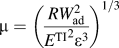
$\mu = {\left( {{{RW_{{\rm{ad}}}^2} \over {{E^{{\rm{TI}}}}^2{\varepsilon ^3}}}} \right)^{1/3}}$
, and the initial air gap can be written as

 $${U_0}(x,y) = {{{X^2} + {Y^2}} \over 2}\quad .$$
-
(ii) For a Berkovich shape, we have
$F = {{{n^2}f} \over {3\pi {m^2}{W_{{\rm{ad}}}}\varepsilon }},\;X = x\left( {{n \over {\varepsilon m}}} \right),\;Y = y\left( {{n \over {\varepsilon m}}} \right)$
, and
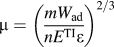
$\mu = {\left( {{{m{W_{{\rm{ad}}}}} \over {n{E^{{\rm{TI}}}}\varepsilon }}} \right)^{2/3}}$
. Note that n/m = 0.133 and the initial air gap can be described as

 $${U_0}(x,y) = \left\{ \matrix{ \sqrt 3 Y + 3\left| X \right|\quad {\rm{if}}\;\,\left| X \right| > - \sqrt 3 Y \hfill \cr 2\sqrt 3 \left| Y \right|\quad {\rm{otherwise}} \hfill \cr} \right.\quad .$$
-
(iii) For a cylindrical flat shape, we have
$F = {{f\varepsilon } \over {3\pi {R^2}{W_{{\rm{ad}}}}}},\;X = {x \over R},\;Y = {y \over R}$
, and
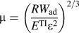
$\mu = {\left( {{{R{W_{{\rm{ad}}}}} \over {{E^{{\rm{TI}}}}{\varepsilon ^2}}}} \right)^{2/3}}$
, and the initial air gap is zero for points (X, Y) inside the circular region
${X^2} + {Y^2} \,\le\, 1$
. -
(iv) For a conical frustum shape, we have
$F = {{f\varepsilon } \over {3\pi \mathop {{R_{\rm{2}}}}\nolimits^2 {W_{{\rm{ad}}}}}},\;X = {x \over {{R_2}}},\;Y = {y \over {{R_2}}}$
, and
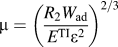
$\mu = {\left( {{{{R_2}{W_{{\rm{ad}}}}} \over {{E^{{\rm{TI}}}}{\varepsilon ^2}}}} \right)^{2/3}}$
, and the initial air gap is zero for points (X, Y) inside the circular region X
2 + Y
2 ≤ 1. For points outside this circular region, we have



 $${U_0}(x,y) = {h \over {{R_1} - {R_2}}}\left[ {{{{R_2}} \over \varepsilon }} \right]\left[ {{{\left( {{X^2} + {Y^2}} \right)}^{{1 \mathord{\left/ {\vphantom {1 2}} \right. \kern-\nulldelimiterspace} 2}}} - 1} \right]\quad .$$
For example, for a conical frustum with a 60° cone angle, we have
 $h/({R_1} - {R_2}) = \sqrt 3$
, and therefore we can obtain
 $${U_0}(x,y) = {{\sqrt 3 {R_2}} \over \varepsilon }\left[ {{{\left( {{X^2} + {Y^2}} \right)}^{{1 \mathord{\left/ {\vphantom {1 2}} \right. \kern-\nulldelimiterspace} 2}}} - 1} \right]\quad .$$
The parameter μ is the so-called Tabor parameter, Reference Tabor31 which is often used to determine whether the JKR or DMT model would best describe a contact system, as Greenwood Reference Greenwood34 concluded that the limits of the Maugis–Dugdale model correspond to Tabor’s limits, with small values of the Tabor parameter describing material behavior in a DMT-type regime, and large values of the Tabor parameter describing the contact behavior for JKR-type regime. Note that the Tabor parameter has different expressions for different types of indenters.
The dimensionless form of Eq. (8b) after tessellation of the problem domain is shown as follows:
 $$H\left( {{X_k},{Y_l}} \right) = - D + {U_0}\left( {{X_k},{Y_l}} \right) + {{{\mu ^{{3 \mathord{\left/ {\vphantom {3 2}} \right. \kern-\nulldelimiterspace} 2}}}} \over \pi }{C_{ij}}\left( {{X_k},{Y_l}} \right){P_{ij}}\quad ,$$
where
 ${C_{ij}}(X,Y) \equiv \int\!\!\!\int_{{\Omega _{ij}}} {{{{\rm{d}}X'\,{\rm{d}}Y'} \over {\sqrt {{{\left( {X - X'} \right)}^2} + {{\left( {Y - Y'} \right)}^2}} }}}$
is the influence coefficient, and P
ij
is the normalized pressure. To write Eq. (12) in a vector form, we have the following equation:
 $$\vec H = - D + {\vec U_0} + {{{\mu ^{{3 \mathord{\left/ {\vphantom {3 2}} \right. \kern-\nulldelimiterspace} 2}}}} \over \pi }C\vec P\quad .$$
Since we assume that the surface interaction is governed by the Lennard-Jones potential,
 $\vec P$
is a highly nonlinear function of
 $\vec H$
. Even for moderately small mesh size where N = 100, the number of elements of C will be the eighth power of ten, and so the computation can rapidly become intractable. To solve this system of N
2 highly nonlinear equations, a VSR method has been used by interposing a virtual dash-pot in the mechanical system. Then Eq. (13) is transformed into the following evolution equation for the dynamical system defined by
 $${{{\rm{d}}\vec H} \over {{\rm{d}}t}} + \vec H = - D + \vec U + {{{\mu ^{{3 \mathord{\left/ {\vphantom {3 2}} \right. \kern-\nulldelimiterspace} 2}}}} \over \pi }C\vec P\quad .$$
The equilibrium solution of this dynamical system is determined by
 ${\rm{d}}\vec H/{\rm{d}}t = \vec 0$
, which is the solution of Eq. (13). In this approach, the indentation depth D is gradually increased, and the H vector obtained from the previous step is used as an initial state for computing the H vector in the next step. In each step, we let time evolve until the final state in equilibrium is reached. This method accurately plots all the stable equilibria for each value of D. In all the simulation cases, we first increase the value of D from the minimum to the maximum indentation depth to simulate the approach process, and then we decrease the value of D back to the minimum to simulate the detachment process.
IV. EXPERIMENTAL METHODS
Indents were performed on a single Sylgard 184 (Dow Corning Corporation, Midland, Michigan) polydimethylsiloxane (PDMS) elastomeric sample prepared following the manufacturer’s instructions. In short, the Sylgard sample was prepared by mixing the PDMS prepolymer base with the curing agent with a weight ratio of 10:1, pouring the mixture into a glass mold, and baking at 70 °C for 3 h. The PDMS sample remained attached to its glass substrate during indentation testing.
Indentation was performed using a Hysitron TI-950 TriboIndenter (Hysitron Inc., Minneapolis, Minnesota) equipped with commercially available diamond tips (Hysitron Inc.). Four tip geometries were used for testing: a 100 μm radius diamond conospherical tip with a 90° cone angle, a diamond Berkovich tip, a 400 μm radius sapphire spherical tip, and a 47 μm radius diamond conical frustum tip with a 60° cone angle.
All indents captured full force curves Reference Kohn and Ebenstein20 in displacement control (100 μm radius spherical tip and Berkovich tip) or open-loop (nominally force control, but without feedback) configuration (400 μm radius spherical tip and flat tip). For displacement control indents, the indenter first detected the surface with a setpoint force of 2 μN, then lifted off from the surface at a rate of −150 nm/s to a height of 1800 nm above the surface (well outside the adhesive interaction zone), and finally indented the sample at a constant displacement rate of 50 nm/s to a maximum depth of 4 μm. For open-loop indents, after the indenter detected the surface with a setpoint force of 2 μN, the tip was manually withdrawn from the surface to between 1.8 and 4.0 μm from the surface, high enough to bring the tip outside the adhesive interaction zone (as indicated by the load on the tip returning to zero), and then an indent was performed from above the surface with an applied load and loading rate that was sufficient to reach a depth of close to 4 μm with a similar rate of loading to the displacement-controlled indents.
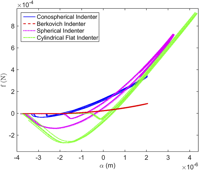
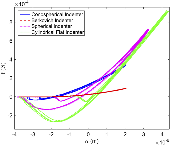
Figure 2 shows typical load–displacement curves obtained by indenting 10:1 PDMS with the four different types of indenters, respectively. Seven curves are shown for the 100 μm radius conospherical tip, six curves are shown for the Berkovich tip, five curves are shown for the 400 μm radius spherical tip, and four curves are shown for the 47 μm radius flat tip. In the numerical simulations, both the conospherical tip and the spherical tip are assumed to be perfectly spherical. The flattened conical tip is often assumed to be a cylindrical flat punch tip at low displacements, and therefore two types of flat indenters are simulated, the cylindrical flat tip and the conical frustum tip, to check if they are significantly different. All the idealized geometries of indenter tips used in the numerical simulations and the corresponding real tips used in the experiments are shown in Fig. 1.
Typical load–displacement curves obtained by indenting 10:1 PDMS with the four different types of indenters, respectively. Seven curves are shown for the 100 μm radius conospherical tip, six curves are shown for the Berkovich tip, five curves are shown for the 400 μm radius spherical tip, and four curves are shown for the 50 μm radius conical frustum tip, illustrating the high repeatability of measurements.
V. RESULTS AND DISCUSSION
A. Spherical indenter
For the spherical shape, recall that
 $F = {f \over {3\pi R{W_{{\rm{ad}}}}}},\;D = {\alpha \over \varepsilon },\;P = {{p\varepsilon } \over {{W_{{\rm{ad}}}}}}$
, and
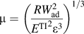 $\mu = {\left( {{{RW_{{\rm{ad}}}^2} \over {{E^{{\rm{TI}}}}^2{\varepsilon ^3}}}} \right)^{1/3}}$
are used in the numerical simulations. We found that when the value of Tabor parameter is 1.5, the numerical results agree very well with the analytical solution derived from the JKR model, as shown in Fig. 3(a), which plots the numerical curves of the normalized force F versus the normalized displacement D for both attachment and detachment processes. Following the standard convention in contact mechanics, we call the absolute value of the minimum force on the load–displacement curve the pull-off or adhesion force, i.e., F
off. From the JKR model, we can obtain that F
off = 0.5. The discrepancies between the numerical results and the analytical solution when the contact radius is small is caused by the fact that when the value of the Tabor parameter is not very small, e.g., μ > 1.0, the contact and separation between two surfaces does not occur smoothly, and there are sudden jumping in or jumping out of contact behaviors.
Reference Greenwood34–Reference Borodich37
When two bodies move closer from a large separation, a turning point exists indicating the jumping-on of contacting surfaces when they move infinitesimally closer. On the other hand, when two bodies are pulled off from a contact state, the turning point corresponds to the jumping-off of contacting surfaces. The middle part between the two turning points represents unstable equilibrium states. The relaxation technique we used can only plot the stable solutions. The unstable solutions, which cannot be observed in real-world experiments, can be obtained by using the Riks arc length method of integration,
Reference Fafard and Massicotte52
but the computational cost will be significantly increased.
(a) The numerical curves of the normalized force F versus the normalized displacement D for spherical indenters for both attachment and detachment processes. It shows that when the value of Tabor parameter is 1.5, the numerical results agree very well with the analytical solution derived from the JKR model. (b) The distribution of the normalized pressure P in the simulation domain [−4.0, 4.0] × [−4.0, 4.0] when the normalized indentation depth D = −2.5, −1.8, −1.0 and 1.0 during approach. (c) The force–displacement curve in a dimensional scale superimposed with the experimental data from nanoindentation tests using the 100 μm radius conospherical tip. We found that
 $W_{{\rm{ad}}}^{{\rm{ap}}} = 0.049$
J/m2,
 $W_{{\rm{ad}}}^{{\rm{de}}} = 0.079$
J/m2, and
 ${E^*} = 2.75$
MPa. (d) The force–displacement curve in a dimensional scale superimposed with the experimental data from nanoindentation tests using the 400 μm radius spherical tip. We found that
 $W_{{\rm{ad}}}^{{\rm{ap}}} = 0.025$
J/m2,
 $W_{{\rm{ad}}}^{{\rm{de}}} = 0.075$
J/m2, and
 ${E^*} = 2.75$
MPa, which are fairly consistent with the results obtained from the case of 100 μm radius conospherical tip.

One of the advantages of conducting numerical simulations is that the pressure distribution within the contact area can be obtained, since there exists no analytical solution for the pressure distribution within the contact region. Figure 3(b) plots the distribution of the normalized pressure P in the simulation domain [−4.0, 4.0] × [−4.0, 4.0] when the normalized indentation depths are D = −2.5, −1.8, −1.0, and 1.0 during approach. Positive values of P represent compressive forces between surfaces, and the edge of the contact area can be regarded as the location of the tensile peak stress, which is colored by the deepest shade of blue in the current color scheme. It can be seen that when the two bodies are approaching each other from a noncontact state, e.g., at D = −2.5, the surfaces barely deform with pressure being nearly zero everywhere. As the two bodies approach each other one step further, e.g., at D = −1.8, the surfaces jump to a new equilibrium state suddenly with a nonzero contact area, and the pressure becomes compressive in the central region and tensile at the contact edge, which is consistent with the results from the previous studies. Reference Greenwood34
A representative loading and unloading force–displacement curve obtained with the 100 μm radius conospherical tip is shown in Fig. 3(c). The observed adhesion hysteresis shows that the work of adhesion during approach, denoted as
 $W_{{\rm{ad}}}^{{\rm{ap}}}$
, is much lower than that during detachment, denoted as
 $W_{{\rm{ad}}}^{{\rm{de}}}$
. Since we have F
off = 0.5, the values of
 $W_{{\rm{ad}}}^{{\rm{ap}}}$
and
 $W_{{\rm{ad}}}^{{\rm{de}}}$
can be calculated from the measured pull-off force
 $f_{{\rm{off}}}^{{\rm{ap}}}$
during approach and
 $f_{{\rm{off}}}^{{\rm{de}}}$
during detachment by using the relationship:
 $W_{{\rm{ad}}}^{{\rm{ap}}} = {2 \over 3}{{f_{{\rm{off}}}^{{\rm{ap}}}} \over {\pi R}}$
and
 $W_{{\rm{ad}}}^{{\rm{de}}} = {2 \over 3}{{f_{{\rm{off}}}^{{\rm{de}}}} \over {\pi R}}$
, respectively. The effective Young’s modulus can be calculated based on two data points from the unloading portion of the curve,
 $f_{{\rm{off}}}^{{\rm{de}}}$
at
 $\alpha _{{\rm{off}}}^{{\rm{de}}}$
(the point where the unloading curve reaches its minimum force) and
 $f_{{\rm{zero}}}^{{\rm{de}}}$
at
 $\alpha _{{\rm{zero}}}^{{\rm{de}}}$
(the point where the unloading force equals zero),
Reference Ebenstein and Wahl9,Reference Ebenstein23
and the relationship obtained from the JKR model:
 ${E^*} = {{0.95f_{{\rm{off}}}^{{\rm{de}}}} \over {\sqrt R }}{\left( {\alpha _{{\rm{zero}}}^{{\rm{de}}} - \alpha _{{\rm{off}}}^{{\rm{de}}}} \right)^{ - 3/2}}$
. Since we can measure that
 $f_{{\rm{off}}}^{{\rm{de}}} = 37.23\;{\rm{\mu N}}$
,
 $f_{{\rm{off}}}^{{\rm{ap}}} = 23.09\;{\rm{\mu N}}$
, and
 $\alpha _{{\rm{zero}}}^{{\rm{de}}} - \alpha _{{\rm{off}}}^{{\rm{de}}} = 1172\;{\rm{nm}}$
, applying these equations to the spherical nanoindentation tests on 10:1 PDMS, we can obtain
 $W_{{\rm{ad}}}^{{\rm{ap}}} = 0.049$
J/m2,
 $W_{{\rm{ad}}}^{{\rm{de}}} = 0.079$
J/m2, and
 ${E^*} = 2.75$
MPa, all of which are reasonable values according to our previous experimental experience.
Reference Jin, Khare, Vajpayee, Yang, Jagota and Hui53
From
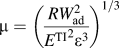 $\mu = {\left( {{{RW_{{\rm{ad}}}^2} \over {{E^{{\rm{TI}}}}^2{\varepsilon ^3}}}} \right)^{1/3}}$
, we can obtain that
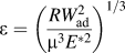 $\varepsilon = {\left( {{{RW_{{\rm{ad}}}^2} \over {{\mu ^3}{E^{*2}}}}} \right)^{1/3}}$
. Since the observed adhesion hysteresis shows that
 $W_{{\rm{ad}}}^{{\rm{ap}}}$
is lower than
 $W_{{\rm{ad}}}^{{\rm{de}}}$
, and we used the same value of the Tabor parameter to simulate both the attachment and detachment processes,
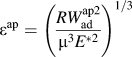 ${\varepsilon ^{{\rm{ap}}}} = {\left( {{{RW_{{\rm{ad}}}^{{\rm{ap}}2}} \over {{\mu ^3}{E^{*2}}}}} \right)^{1/3}}$
should be smaller than
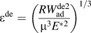 ${\varepsilon ^{{\rm{de}}}} = {\left( {{{RW_{{\rm{ad}}}^{{\rm{de}}2}} \over {{\mu ^3}{E^{*2}}}}} \right)^{1/3}}$
. Figure 3(c) shows the force–displacement curve in a dimensional scale superimposed with the experimental data.
A representative loading and unloading force–displacement curve obtained with the 400 μm radius spherical tip is shown in Fig. 3(d). Since we can measure that
 $f_{{\rm{off}}}^{{\rm{de}}} = 141.20\;{\rm{\mu N}}$
,
 $f_{{\rm{off}}}^{{\rm{ap}}} = 47.67\;{\rm{\mu N}}$
, and
 $\alpha _{{\rm{zero}}}^{{\rm{de}}} - \alpha _{{\rm{off}}}^{{\rm{de}}} = 1810\;{\rm{nm}}$
, substituting these values into the nano-JKR force curve equations, we can obtain that
 $W_{{\rm{ad}}}^{{\rm{ap}}} = 0.025$
J/m2,
 $W_{{\rm{ad}}}^{{\rm{de}}} = 0.075$
J/m2, and
 ${E^*} = 2.75$
MPa, which are fairly consistent with the results obtained from the case of the 100 μm radius conospherical tip. Figure 3(d) shows the force–displacement curve in a dimensional scale superimposed with the experimental data.
B. Berkovich indenter
For the Berkovich shape, recall that
 $F = {{{n^2}f} \over {3\pi {m^2}{W_{{\rm{ad}}}}\varepsilon }},\;D = {\alpha \over \varepsilon },\;P = {{p\varepsilon } \over {{W_{{\rm{ad}}}}}}$
, and
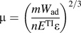 $\mu = {\left( {{{m{W_{{\rm{ad}}}}} \over {n{E^{{\rm{TI}}}}\varepsilon }}} \right)^{2/3}}$
are used in the numerical simulation. Figure 4(a) plots the numerical simulation curves of the normalized force F versus the normalized displacement D for both attachment and detachment processes when the value of the Tabor parameter is equal to 1.5. Since there exists no analytical solution for the force–displacement relationship for Berkovich indenters, these important values will be directly measured from the numerical simulation curve. The normalized pull-off force can be obtained as F
off = 0.21, the unloading force reaches its minimum at
 $D_{{\rm{off}}}^{{\rm{de}}} = 1.59$
, and when the unloading force equals zero,
 $D_{{\rm{zero}}}^{{\rm{de}}} = 5.31$
. These values will be used in calculating
 $W_{{\rm{ad}}}^{{\rm{ap}}}$
,
 $W_{{\rm{ad}}}^{{\rm{de}}}$
, and
 ${E^*}$
. The jumping in and jumping out of contact behaviors are not as obvious, because during the nanoindentation tests using Berkovich indenters, the contact area at a given amount of indentation depth is much smaller than that during the tests using spherical indenters.
(a) The numerical curves of the normalized force F versus the normalized displacement D for Berkovich indenters for both attachment and detachment processes. The value of Tabor parameter is set to be 1.5. (b) The distribution of the normalized pressure P in the simulation domain [−6.7, 6.7] × [−6.7, 6.7] when the normalized indentation depth D = −2.5, 2.5, 5.5, and 7.5 during approach. (c) The force–displacement curve in a dimensional scale superimposed with the experimental data from nanoindentation tests using Berkovich indenters. We found that
 $W_{{\rm{ad}}}^{{\rm{ap}}} = 0.055$
J/m2,
 $W_{{\rm{ad}}}^{{\rm{de}}} = 0.077$
J/m2, and
 ${E^*} = 2.48$
MPa.

Figure 4(b) plots the distribution of the normalized pressure P in the simulation domain [−6.7, 6.7] × [−6.7, 6.7] when the normalized indentation depths are D = −2.5, 2.5, 5.5, and 7.5 during approach. It can be seen that when the two bodies are approaching each other from a noncontact state, e.g., at D = −2.5, the surfaces barely deform with pressure being nearly zero everywhere. As the two bodies approach each other further, e.g., at D = 2.5, the surfaces obtain an equilibrium state with a nonzero contact area. For the Berkovich tip, the compressive contact pressure forms a sharp peak at the center, and therefore the values of the contact pressure at the center of the contact region become much larger than those obtained by using the spherical indenter.
A complete loading and unloading force–displacement curve obtained with the Berkovich tip has been shown in Fig. 4(c). Since we have F
off = 0.21, the relationship of
 $W_{{\rm{ad}}}^{{\rm{ap}}}$
and
 $W_{{\rm{ad}}}^{{\rm{de}}}$
with the measured pull-off force
 $f_{{\rm{off}}}^{{\rm{ap}}}$
during approach and
 $f_{{\rm{off}}}^{{\rm{de}}}$
during detachment can be written as
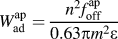 $W_{{\rm{ad}}}^{{\rm{ap}}} = {{{n^2}f_{{\rm{off}}}^{{\rm{ap}}}} \over {0.63\pi {m^2}\varepsilon }}$
and
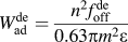 $W_{{\rm{ad}}}^{{\rm{de}}} = {{{n^2}f_{{\rm{off}}}^{{\rm{de}}}} \over {0.63\pi {m^2}\varepsilon }}$
, respectively. From
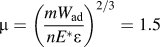 $\mu = {\left( {{{m{W_{{\rm{ad}}}}} \over {n{E^*}\varepsilon }}} \right)^{2/3}} = 1.5$
, we can obtain that
 $\varepsilon = {{m{W_{{\rm{ad}}}}} \over {1.84n{E^*}}}$
. Since
 $W_{{\rm{ad}}}^{{\rm{ap}}}$
is lower than
 $W_{{\rm{ad}}}^{{\rm{de}}}$
,
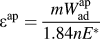 ${\varepsilon ^{{\rm{ap}}}} = {{mW_{{\rm{ad}}}^{{\rm{ap}}}} \over {1.84n{E^*}}}$
should be smaller than
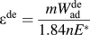 ${\varepsilon ^{{\rm{de}}}} = {{mW_{{\rm{ad}}}^{{\rm{de}}}} \over {1.84n{E^*}}}$
. We then have the following equations, respectively:
 $$W_{{\rm{ad}}}^{{\rm{ap}}} = {\left( {{{2.92{n^3}f_{{\rm{off}}}^{{\rm{ap}}}{E^*}} \over {\pi {m^3}}}} \right)^{1/2}}\quad ,$$
 $$W_{{\rm{ad}}}^{{\rm{de}}} = {\left( {{{2.92{n^3}f_{{\rm{off}}}^{{\rm{de}}}{E^*}} \over {\pi {m^3}}}} \right)^{1/2}}\quad .$$
Since the numerical simulation curve shows that
 $D_{{\rm{zero}}}^{{\rm{de}}} - D_{{\rm{off}}}^{{\rm{de}}} = 3.72$
, we have
 $\alpha _{{\rm{zero}}}^{{\rm{de}}} - \alpha _{{\rm{off}}}^{{\rm{de}}} = 3.72\varepsilon$
, and then we can obtain the following relationship:
 $$\alpha _{{\rm{zero}}}^{{\rm{de}}} - \alpha _{{\rm{off}}}^{{\rm{de}}} = {{2.02mW_{{\rm{ad}}}^{{\rm{de}}}} \over {n{E^*}}}\quad .$$
As measured from the representative experimental curve shown in Fig. 4(c), we obtain that
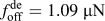 $f_{{\rm{off}}}^{{\rm{de}}} = 1.09\;\mu {\rm{N}}$
,
 $f_{{\rm{off}}}^{{\rm{ap}}} = 0.55\;\mu {\rm{N}}$
, and
 $\alpha _{{\rm{zero}}}^{{\rm{de}}} - \alpha _{{\rm{off}}}^{{\rm{de}}} = 472\;{\rm{nm}}$
. Remember that for the Berkovich tip, we always have n/m = 0.133. Substituting these values into Eqs. (15)–(17), we can obtain that
 $W_{{\rm{ad}}}^{{\rm{ap}}} = 0.055$
J/m2,
 $W_{{\rm{ad}}}^{{\rm{de}}} = 0.077$
J/m2, and
 ${E^*} = 2.48$
MPa, which are fairly consistent with the results we obtained from the experiments using the spherical indenter. Several factors, different in nature, could explain the discrepancy in the modulus results. First, slight variations from the ideal geometries used in the numerical simulations would be expected for the real tips, due to blunted points in Berkovich tips and the fact that diamond tips are never perfectly spherical. This in turn can lead to some error in modulus calculation when conducting numerical simulations based on idealized tip geometries to analyze experimental data collected using real tips. Second, in numerical simulations, Derjaguin’s approximation is used to calculate surface tractions, which is not the exact adhesion. If the Derjaguin assumptions are not accepted and/or there is friction at the edge of the contact region then the adhesive forces can work on tangential displacements and the mode-mixity effects have to be discussed; however, as Borodich et al. noted,
Reference Borodich, Galanov and Suarez-Alvarez54
interaction between adhesion and friction under both static and kinetic conditions is still an open question. Finally, the formulas used in the numerical simulation are restricted in the small strain range and linear elastic material behavior. Figure 4(c) shows the force–displacement curve in a dimensional scale superimposed with the experimental data.
It is important to note that Eqs. (15), (16), and (17) can also be used to determine reduced modulus and work of adhesion for a compliant material from nanoindentation tests using cube-corner indenter.
Reference Deuschle, Buerki, Deuschle, Enders, Michler and Arzt15
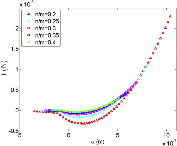
As the name implies, a cube corner tip is a three-sided pyramidal tip with perpendicular faces like the corner of a cube. The centerline-to-face angle is 35.3°, much sharper than a Berkovich pyramid. When the value of the Tabor parameter is 1.5, the numerical simulation results of the normalized force F versus the normalized displacement D for both attachment and detachment processes will be the same as the curve shown in Fig. 4(c), which is obtained from Berkovich indenters; however, in the case of cube-corner indenters, we have n/m = 0.408, and therefore the curve of the dimensional force f versus the dimensional displacement α will be different. To explore the effect of different ratios of n and m of a three-sided pyramidal tip on the dimensional force–displacement curve, we plot five different curves for nanoindentation tests on a compliant material with W
ad = 0.077 J/m2 and
 ${E^*} = 2.48$
MPa, as shown in Fig. 5, corresponding to five different pyramidal tips with n/m equal to 0.2, 0.25, 0.3, 0.35, and 0.4, respectively. It can be seen that the absolute value of the minimum force decreases monotonically with increasing values of n/m, which is consistent with experimental observations.
Reference Deuschle, Buerki, Deuschle, Enders, Michler and Arzt15
Five different loading curves for nanoindentation tests on a compliant material with W
ad = 0.077 J/m2 and
 ${E^*} = 2.48$
MPa, corresponding to five different pyramidal tips with n/m equal to 0.2, 0.25, 0.3, 0.35, and 0.4, respectively.
By assuming that the value of the Tabor parameter is equal to 1.5, the numerical simulations have been so far carried out only in the JKR adhesion regime.
Reference Spolenak, Gorb, Gao and Arzt55
In the JKR-type contact problems, an important assumption is that the surface interaction is absent outside the contact area. The DMT theory deploys cohesive surface forces outside the contact zone, while retaining the Hertzian force-deformation characteristics in the core.
Reference Johnson26
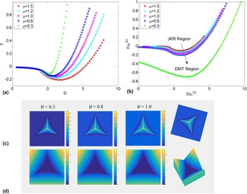
This results in the adhesive stress being zero inside the contact area and finite outside it. To explore the DMT-type regimes and the JKR-DMT transition regimes, nanoindentation tests using Berkovich indenters are simulated for five different values of the Tabor parameter: 0.3, 0.8, 1.0, 1.2, and 1.5. Figure 6(a) plots the normalized force F versus normalized displacement D. Since we have
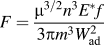 $F = {{{\mu ^{3/2}}{n^3}{E^*}f} \over {3\pi {m^3}W_{{\rm{ad}}}^2}}$
and
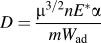 $D = {{{\mu ^{3/2}}n{E^*}\alpha } \over {m{W_{{\rm{ad}}}}}}$
, Fig. 6(b) plots the normalized force Fμ−3/2 versus normalized displacement Dμ−3/2, which shows that with decreasing values of the Tabor parameter, the force–displacement curve goes from the JKR regime to the DMT regime.
Reference Borodich37
Figure 6(c) plots a series of normalized pressure distributions in the simulation domain [−7.0, 7.0] × [−7.0, 7.0] when the normalized indentation depth D = 10.0 during approach. This simulation has been performed by using three different values of the Tabor parameter: 0.3, 0.8, and 1.0. It can be seen that when the value of the Tabor parameter is small, very large values of P can be observed at the center of the contact region. Figure 6(d) plots the normalized air gap between the indenter surface and the sample surface H in the simulation domain [−7.0, 7.0] × [−7.0, 7.0] when D = 10.0 during approach. During loading, a clear sink-in effect
Reference McElhaney, Vlassak and Nix56
is visible as indicated by the curved contact edge, which is consistent with experimental observations from in situ nanoindentation testing of PDMS samples using Berkovich tips.
Reference Deuschle, Buerki, Deuschle, Enders, Michler and Arzt15
(a) The numerical simulation results of the normalized force F versus the normalized displacement D during attachment for Berkovich indenters using five different values of the Tabor parameter: 0.3, 0.8, 1.0, 1.2, and 1.5. (b) The numerical simulation results of the normalized force Fμ−3/2 versus the normalized displacement Dμ−3/2 during attachment. (c) Normalized pressure distributions P in the simulation domain [−7.0, 7.0] × [−7.0, 7.0] when the normalized indentation depth D = 10.0 during attachment using three different values of Tabor parameter: 0.3, 0.8, and 1.0. (d) Normalized air gap between the two surfaces H in the simulation domain [−7.0, 7.0] × [−7.0, 7.0] when the normalized indentation depth D = 10.0 during attachment.

C. Cylindrical flat indenter
For the cylindrical flat indenter, recall that
 $F = {{f\varepsilon } \over {3\pi {R^2}{W_{{\rm{ad}}}}}},\;D = {\alpha \over \varepsilon },\;P = {{p\varepsilon } \over {{W_{{\rm{ad}}}}}}$
, and
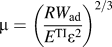 $\mu = {\left( {{{R{W_{{\rm{ad}}}}} \over {{E^{{\rm{TI}}}}{\varepsilon ^2}}}} \right)^{2/3}}$
are used in the numerical simulation. Figure 7(a) plots the numerical simulation curves of the normalized force F versus the normalized displacement D for both attachment and detachment processes when the value of the Tabor parameter is equal to 1.5. The jumping in and jumping out of contact behaviors are clearly observed. Just like the case of the Berkovich indenter, there exists no analytical solution for the force–displacement relationship, and thus these important values will be directly measured from the numerical simulation curve. The absolute value of the minimum force on the loading curve can be obtained as
 $F_{{\rm{off}}}^{{\rm{ap}}} = 0.21$
, the normalized pull-off force from the unloading curve can be obtained as
 $F_{{\rm{off}}}^{{\rm{de}}} = 0.25$
, and the unloading portion is a straight line of slope S = 0.114. These three important values will be used in calculating
 $W_{{\rm{ad}}}^{{\rm{ap}}}$
,
 $W_{{\rm{ad}}}^{{\rm{de}}}$
, and
 ${E^*}$
. Note that in this case, the values of
 $F_{{\rm{off}}}^{{\rm{ap}}}$
and
 $F_{{\rm{off}}}^{{\rm{de}}}$
are not exactly the same.
(a) The numerical curves of the normalized force F versus the normalized displacement D for cylindrical flat indenters for both attachment and detachment processes. The value of Tabor parameter is set to be 1.5. (b) The force–displacement curve in a dimensional scale superimposed with the experimental data from nanoindentation tests using conical frustum indenters. We found that
 $W_{{\rm{ad}}}^{{\rm{ap}}} = 0.001$
J/m2,
 $W_{{\rm{ad}}}^{{\rm{de}}} = 0.027$
J/m2, and
 ${E^*} = 2.47$
MPa. (c) The numerical simulation curves of the normalized force F versus the normalized displacement D for conical frustum indenters for both attachment and detachment processes for three different values of
 ${{{R_2}} \over \varepsilon }$
when the value of the Tabor parameter is equal to 1.5. (d) The distribution of the normalized pressure P in the simulation domain [−2.0, 2.0] × [−2.0, 2.0] for conical frustum indenters when
 ${{{R_2}} \over \varepsilon } = 5$
and
 ${{{R_2}} \over \varepsilon } = 12$
as the normalized indentation depths are D = −5.0, 1.0, 4.0, and 7.0 during approach.

A complete loading and unloading force–displacement curve obtained with the cylindrical flat tip has been shown in Fig. 7(b). Since we have
 $F_{{\rm{off}}}^{{\rm{ap}}} = 0.21$
and
 $F_{{\rm{off}}}^{{\rm{de}}} = 0.25$
, the relationship of
 $W_{{\rm{ad}}}^{{\rm{ap}}}$
and
 $W_{{\rm{ad}}}^{{\rm{de}}}$
with the measured pull-off force
 $f_{{\rm{off}}}^{{\rm{ap}}}$
during approach and
 $f_{{\rm{off}}}^{{\rm{de}}}$
during detachment can be written as
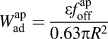 $W_{{\rm{ad}}}^{{\rm{ap}}} = {{\varepsilon f_{{\rm{off}}}^{{\rm{ap}}}} \over {0.63\pi {R^2}}}$
and
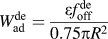 $W_{{\rm{ad}}}^{{\rm{de}}} = {{\varepsilon f_{{\rm{off}}}^{{\rm{de}}}} \over {0.75\pi {R^2}}}$
, respectively. From
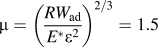 $\mu = {\left( {{{R{W_{{\rm{ad}}}}} \over {{E^*}{\varepsilon ^2}}}} \right)^{2/3}} = 1.5$
, we can obtain that
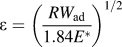 $\varepsilon = {\left( {{{R{W_{{\rm{ad}}}}} \over {1.84{E^*}}}} \right)^{1/2}}$
. We then have the following equations, respectively:
 $$W_{{\rm{ad}}}^{{\rm{ap}}} = {{{{\left( {f_{{\rm{off}}}^{{\rm{ap}}}} \right)}^2}} \over {0.73{\pi ^2}{E^*}{R^3}}}\quad ,$$
 $$W_{{\rm{ad}}}^{{\rm{de}}} = {{{{\left( {f_{{\rm{off}}}^{{\rm{de}}}} \right)}^2}} \over {1.04{\pi ^2}{E^*}{R^3}}}\quad .$$
Since the unloading portion is a straight line of slope S = 0.114, we can obtain the following relationship:
 $${E^*} = {s \over {5.51\pi RS}}\quad ,$$
where s is the slope of the unloading portion measured from the experimental curve. As measured from the representative curve shown in Fig. 7(b), we obtain that
 $f_{{\rm{off}}}^{{\rm{de}}} = 266.60\;\mu {\rm{N}}$
,
 $f_{{\rm{off}}}^{{\rm{ap}}} = 51.35\;\mu {\rm{N}}$
, and the slope of the unloading portion can be obtained as s = 228.9. Substituting these values, along with R = 47 μm, into Eqs. (18)–(20), we can obtain that
 $W_{{\rm{ad}}}^{{\rm{ap}}} = 0.001$
J/m2,
 $W_{{\rm{ad}}}^{{\rm{de}}} = 0.027$
J/m2, and
 ${E^*} = 2.47$
MPa. The value of the reduced modulus is fairly consistent with the result we obtained from the experiments using the Berkovich indenter. Note that the cylindrical flat indentation models, i.e., Eqs. (18)–(20), are accurate only if the flattened tip is perfectly parallel to the sample surface so that full contact is achieved during the indent process, but full contact is difficult to establish experimentally due to the unavoidable sample tilt with respect to the flat punch surface.
Reference De Paoli and Volinsky17
It is interesting to notice that if
 ${E^*}$
is calculated by assuming there is negligible adhesion and therefore using,
 ${E^*} = {s \over {2R}}$
Reference Wang, Volinsky and Gallant16
almost an identical modulus can be obtained according to Eq. (20), since 5.51πS ≈ 2. Hence, adhesion seems to be negligible in this scenario, which is consistent with the extremely low value of
 $W_{{\rm{ad}}}^{{\rm{ap}}}$
(only 0.001 J/m2) observed during sample approach for the cylindrical flat tip.
Figure 7(b) shows the force–displacement curve in a dimensional scale superimposed with the experimental data. It can be observed that the simulation curve does not track the experimental curve well during the final stages of retraction of the tip. This is because the model assumes that full contact with the flat tip is maintained throughout tip retraction until pull-off, resulting in a linear unloading curve until pull-off. The experimental curve shows a linear region at the beginning of the unloading curve, indicating a constant area of contact during initial tip retraction, but becomes nonlinear as the load approaches 0 μN. This nonlinearity suggests that the contact size is gradually changing during the later stages of retraction, which would be expected if the tip is not perfectly parallel to the sample surface and the tip detaches from the sample gradually rather than breaking the entire circular contact at once.
D. Conical frustum indenter
For the conical frustum indenter, recall that
 $F = {{f\varepsilon } \over {3\pi \mathop {{R_{\rm{2}}}}\nolimits^2 {W_{{\rm{ad}}}}}},\;D = {\alpha \over \varepsilon },\;P = {{p\varepsilon } \over {{W_{{\rm{ad}}}}}}$
, and
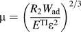 $\mu = {\left( {{{{R_2}{W_{{\rm{ad}}}}} \over {{E^{{\rm{TI}}}}{\varepsilon ^2}}}} \right)^{2/3}}$
are used in the numerical simulation. Figure 7(c) plots the numerical simulation curves of the normalized force F versus the normalized displacement D for both attachment and detachment processes for three different values of
 ${{{R_2}} \over \varepsilon }$
when the value of the Tabor parameter is equal to 1.5. It can be seen that when
 ${{{R_2}} \over \varepsilon } \,\ge\, 50$
, the numerical simulation curve shows almost no difference from the one we obtained from the case of the cylindrical flat tip. From the simulation for the cylindrical flat tip, we obtained that
 $W_{{\rm{ad}}}^{{\rm{ap}}} = 0.001$
J/m2,
 $W_{{\rm{ad}}}^{{\rm{de}}} = 0.027$
J/m2, and
 ${E^*} = 2.47$
MPa. Substituting these values into
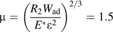 $\mu = {\left( {{{{R_2}{W_{{\rm{ad}}}}} \over {{E^*}{\varepsilon ^2}}}} \right)^{2/3}} = 1.5$
, we can obtain that
 ${{{R_2}} \over {{\varepsilon ^{{\rm{ap}}}}}} = 462$
and
 ${{{R_2}} \over {{\varepsilon ^{{\rm{de}}}}}} = 89$
, both of which are larger than 50, indicating that the conical frustum tip we used in the experiments can be safely regarded as a cylindrical flat punch for shallow indentations. When
 ${{{R_2}} \over {\rm{\varepsilon }}} = 5$
, the numerical simulation curve shows obvious deviation from the curve for the cylindrical flat tip, and therefore in this case the conical frustum tip cannot be considered as a cylindrical flat punch even for shallow indentations. Figure 7(d) plots the distribution of the normalized pressure P in the simulation domain [−2.0, 2.0] × [−2.0, 2.0] when
 ${{{R_2}} \over \varepsilon } = 5$
and
 ${{{R_2}} \over \varepsilon } = 12$
as the normalized indentation depths are D = −5.0, 1.0, 4.0 and 7.0 during approach, respectively. The plots suggest that when the value of
 ${{{R_2}} \over \varepsilon }$
is small, e.g.,
 ${{{R_2}} \over \varepsilon } = 5$
, the sample contacts not only the flattened end of the conical frustum tip but also the sides of the cone during indentation, consistent with the reported experimental results for indentation of polyacrylamide hydrogels using a conical frustum tip at large indentation depths.
Reference Tong and Ebenstein19
As the value of
 ${{{R_2}} \over \varepsilon }$
is increased from 5 to 12, a smaller part of the sides of the cone comes in contact with the sample.
E. Comparison with existing literature
The reduced modulus values determined from the experimental data reported in this study range from 2.47 to 2.75 MPa. The mechanical properties of Sylgard 184 PDMS have been shown to be sensitive to the weight percentage of the crosslinker, curing time, and curing temperature, so the mechanical properties of the PDMS samples from different batches may not be exactly the same. For example, one study on 10:1 Sylgard 184 PDMS conducted by Johnston et al. Reference Johnston, McCluskey, Tan and Tracey57 showed that the elastic modulus increased from 1.32 to 2.97 MPa as curing temperature increased from 25 °C to 200 °C. This range of moduli correspond to reduced modulus values between 1.76 and 3.96 MPa if ν = 0.5 is assumed. A mean reduced modulus of 2.73 MPa was reported for the samples cured for 48 min at 100 °C, which is quite consistent with the values presented in the current study. In another study, Sharfeddin et al. Reference Sharfeddin, Volinsky, Mohan and Gallant58 measured elastic properties of Sylgard 184 PDMS samples at different scales with the 10:1 to 50:1 elastomer base to the curing agent ratios. Macroscopic compression and tension tests were compared with the nano-JKR force curve method applied to spherical microindentation tests. They showed that the PDMS elastic modulus varied as a sigmoid function with the crosslinking percentage for each type of test. For 10:1 PDMS samples cured for 20 h at 65 °C, they reported that the mean reduced modulus was approximately 2.33 MPa (if ν = 0.5 is assumed) based on the results from both macroscale compression tests and microscale indentation tests, which is quite close to the results reported here.
Since the values of
 $W_{{\rm{ad}}}^{{\rm{ap}}}$
and
 $W_{{\rm{ad}}}^{{\rm{de}}}$
depend on the rate at which the contact area is increasing and decreasing,
Reference Shull59
respectively, it is expected that the values
 $W_{{\rm{ad}}}^{{\rm{ap}}}$
and
 $W_{{\rm{ad}}}^{{\rm{de}}}$
will be different for different shapes of indenters. The values of
 $W_{{\rm{ad}}}^{{\rm{ap}}}$
and
 $W_{{\rm{ad}}}^{{\rm{de}}}$
obtained from the spherical nanoindentation in the current study are found to be fairly consistent with the values in the existing literature. For example, Yu et al.
Reference Yu, Sanchez and Lu60
conducted more than one hundred JKR experiments by using a dynamical mechanical analyzer to measure the values of
 $W_{{\rm{ad}}}^{{\rm{ap}}}$
and
 $W_{{\rm{ad}}}^{{\rm{de}}}$
of Sylgard 184 PDMS samples with five different mixing ratios. They showed that the measured values of
 $W_{{\rm{ad}}}^{{\rm{ap}}}$
and
 $W_{{\rm{ad}}}^{{\rm{de}}}$
for 10:1 PDMS cured for 24 h at 120 °C were 0.040–0.044 J/m2 and 0.061–0.068 J/m2, respectively.
VI. CONCLUSION
In this paper, we have successfully extended the nano-JKR force curve method to include Berkovich indenters and flat indenters by conducting a numerical simulation in which the adhesive interactions are represented by an interaction potential and the surface deformations are coupled by using half-space Green’s functions discretized on the surface. This method provides a valuable approach to analyze tip-sample contacts to polymers or other compliant materials. The good agreement between the experimental data and the theoretical prediction have confirmed that this approach can be used to accurately determine reduced modulus and work of adhesion during both approach and detachment for a compliant polymer under conditions where there are strong adhesive forces between the tip and the sample. The DMT-type and JKR-type-to-DMT-type transition regimes have been explored by conducting the simulations using smaller values of Tabor parameters, and those results can be used to study contact problems involving stiff materials, small sphere radii and weak, long-range adhesion forces. This numerical simulation package can be easily extended to study nanoindentation tests using other types of indenters, such as cube-corner indenters, Vickers indenters, Reference Smith and Sutherland61 Knoop indenters, Reference Knoop, Peters and Emerson62 and conical indenters, which will be of significant importance for mechanical characterization of polymeric and biological materials. However, the results presented in this paper assume that the contacting materials have well-defined elastic constants. In fact, most materials have at least some viscoelastic character, and in our future work, these effects will be taken into account.
ACKNOWLEDGMENTS
This work is supported by start-up funds provided by the Department of Mechanical Engineering at State University of New York at Binghamton. The nanoindenter used in this study was obtained through the support of the National Science Foundation (MRI-1040319). Conclusions and recommendations expressed in this paper are those of the authors and do not necessarily reflect the views of the National Science Foundation.