1. Introduction
It is well known that forecasters disagree in their views about future inflation (Mankiw et al., Reference Mankiw, Reis, Wolfers, Mankiw, Reis and Wolfers2003; Dovern et al., Reference Dovern, Fritsche and Slacalek2012; Andrade et al., Reference Andrade, Crump, Eusepi and Moench2016; Fofana et al., Reference Fofana, Patzelt and Reis2024). The extent of disagreement varies over time, is related to the business cycle and prevails even under credible monetary policy regimes such as inflation targeting. Disagreement is not limited to forecasts made by households but also characterizes professional forecasters.
In this paper, we investigate whether disagreement about future inflation affects the monetary transmission mechanism in Korea. Since 1998, the Bank of Korea (BOK) has successfully pursued inflation targeting.Footnote 1 We measure disagreement by the cross-sectional dispersion of forecasts about one-year ahead inflation from the Consensus Economics panel. During the period from 2006 to 2023, disagreement has fluctuated over time and reached a maximum in 2009 during the global financial crisis and a minimum in 2018.
Based on a series of estimated state-dependent local projections (Jordà, Reference Jordà2005; Auerbach and Gorodnichenko, Reference Auerbach, Gorodnichenko, Auerbach and Gorodnichenko2013; Tenreyro and Thwaites, Reference Tenreyro and Thwaites2016) and high-frequency monetary policy shocks, we show that higher levels of disagreement dampen the transmission of monetary impulses. If disagreement is low, the responses of inflation, inflation expectations, and real activity are consistent with textbook predictions. Hence, a policy tightening reduces actual and expected inflation, increases unemployment, and leads to lower growth in industrial production and a lower expected growth rate of GDP. If disagreement is high, monetary policy becomes ineffective as most responses become insignificant or even have the wrong sign. Bems et al. (Reference Bems, Caselli, Grigoli and Gruss2021) use the cross-sectional dispersion of inflation expectations as a measure of de-anchoring of inflation expectations. Based on their interpretation of forecast dispersion, our results suggest that monetary policy becomes ineffective in a regime of de-anchored inflation expectations.
Our finding of weakened monetary transmission effect under high disagreement is in line with Falck et al. (Reference Falck, Hoffmann and Hürtgen2021) that attribute the reduced effectiveness of monetary policy to a changing relative size of the signaling channel of monetary transmission. They estimate state-dependent local projections using time-varying disagreement of expected inflation in the U.S. Survey of Professional Forecasters and find that a contractionary monetary policy shock increases inflation and expected inflation if disagreement is high, but reduces inflation and expected inflation if disagreement is low. To explain state-dependent effects of monetary policy, they extend a New Keynesian model with dispersed information (Melosi, Reference Melosi2017) of price-setters by exogenous shifts in the precision of information, which delivers fluctuations in disagreement, and investigate a signaling channel of monetary policy. They show that, under high disagreement, a surprise tightening can be interpreted as a signal about a better-than-expected state of the economy. This channel dominates the conventional transmission channel. As a result, firms set a higher price. Conversely, if disagreement is low, this signaling effect becomes weak and is dominated by the conventional channel of monetary policy transmission. Hence, firms set lower prices.Footnote 2
This paper is also closely related to Barbera et al. (Reference Barbera, Xia and Zhu2023) and Esady (Reference Esady2022). Barbera et al. (Reference Barbera, Xia and Zhu2023) use data for the U.S. on the term structure of inflation forecast disagreement in order to distinguish between disagreement about the inflation trend and disagreement about cyclical inflation. They show that the cyclical part of disagreement weakens monetary policy transmission, but not disagreement about long-run inflation. In contrast to the Falck et al. (Reference Falck, Hoffmann and Hürtgen2021) and Barbera et al. (Reference Barbera, Xia and Zhu2023), Esady (Reference Esady2022) uses data on the disagreement of the U.S. Survey of Professional Forecasters about the nowcast of real GDP. This serves as a proxy for information rigidities across forecasters. She finds that a policy tightening has a smaller effect on inflation if disagreement is high.
We extend this line of research in three dimensions. First, we show that the state-dependent effects of monetary policy driven by time-variation in forecast disagreement hold not only for advanced economies but also for Korea, which transitioned from an emerging to an advanced economy over the past two decades. In addition, the Korean economy is heavily exposed to spillover effects from global monetary and financial conditions. Thus, it is essential to examine whether emerging markets and small open economies share the pattern where inflation disagreement dampens monetary policy effects, as in the case of advanced economies. However, there exist only a few studies examining these effects on emerging and small open economies. For example, Kwon and Shin (Reference Kwon and Shin2023) find that the exchange rate pass-through depends on the extent of forecast disagreement, but their analysis does not include the transmission of monetary policy impulses. We contribute to the literature by showing that, in Korea, high disagreement on inflation expectations can significantly reduce or distort monetary policy effects, consistent with the previous findings for advanced economies.
Second, we show that the state-dependent effects of monetary policy in our baseline model are not merely reflecting the change in the type of the BOK’s inflation target from range to point target. This is important as the fall in disagreement of forecasters about future inflation coincides with the shift by the BOK from a target range to a point target for inflation. When additionally conditioning the strength of the responses to monetary policy on the definition of the inflation target, the unconditional effect of a monetary policy shock still depends on the level of forecast disagreement about inflation. Thus, our findings are also related to the literature on the relationship between the design of inflation targeting types and the dispersion of inflation forecasts (Capistran and Ramos-Francia, Reference Capistran and Ramos-Francia2010; Gürkaynak et al., Reference Gürkaynak, Levin and Swanson2010; Dovern et al., Reference Dovern, Fritsche and Slacalek2012; Ehrmann, Reference Ehrmann2021).
Third, we distinguish the effect of forecast disagreement from the effect of monetary policy uncertainty. The latter is also known to influence the effectiveness of monetary policy (Tillmann, Reference Tillmann2020). In fact, the literature often uses fluctuations in disagreement as a proxy for subjective uncertainty (Bachmann et al., Reference Bachmann, Elstner and Sims2013), though disagreement and uncertainty are related, but distinct concepts (Lahiri and Sheng, Reference Lahiri and Sheng2010; Glas and Hartmann, Reference Glas and Hartmann2016; Glas, Reference Glas2020; Zohar, Reference Zohar2023). We augment our model and allow the measure of monetary policy uncertainty of Cho and Kim (Reference Cho and Kim2023) to be an additional factor that could moderate the effects of monetary policy. We show that our results remain unchanged if we account for fluctuations in uncertainty.
Our findings imply that central banks should develop communication strategies aimed at reducing dispersion over inflation expectations to enhance the monetary transmission effects and, consequently, to achieve macroeconomic stability. A recent paper, Ascari et al. (Reference Ascari, Bonomolo and Celani2024), also highlights that an increased dispersion of inflation expectations weakens the macroeconomic condition even more than an increase in average inflation expectations.
The remainder of this paper is structured as follows. Section 2 introduces our measures of inflation disagreement. Section 3 explains the empirical model and the identification of monetary policy shock, while Section 4 discusses the main empirical results. Section 5 introduces additional moderating effects, i.e., uncertainty, the changing nature of the BOK’s inflation targeting type, or other variables from the Consensus Economics panel. Section 6 concludes.
2. Inflation disagreement in Korea
Our main data source for inflation expectations is the monthly survey conducted by Consensus Economics among major financial institutions.Footnote 3 Throughout our sample period, from January 2006 to November 2023, between 14 and 21 respondents from banks and asset managing firms provide their assessment of inflation in the current and next calendar years.Footnote 4
The forecasts are fixed-event forecasts. Hence, each forecaster submits his or her projection for inflation at the end of the current and the next year. We follow the literature (Siklos, Reference Siklos2013; Dovern et al., Reference Dovern, Fritsche and Slacalek2012; Gerlach, Reference Gerlach2007) and transform these forecasts into fixed-horizon forecasts, i.e., the projected inflation one year ahead. Specifically, we approximate the one-year ahead inflation forecast as a weighted sum of current and next calendar year forecasts,
 $[(13-m)/12]\pi ^{FE}_{m,t}+[(m-1)/12]\pi ^{FE}_{m,t+1}$
where
 $\pi ^{FE}_{m,t}$
and
 $\pi ^{FE}_{m,t+1}$
denote fixed event inflation forecasts for
 $t$
and
 $t+1$
calendar years released in month
 $m$
of year
 $t$
. For example, in March 2009, the one-year ahead inflation forecast is approximated by the sum of the inflation forecasts for the current and next calendar years released in March 2009, weighted by
 $10/12$
and
 $2/12$
, respectively.
From this set of forecasts, we use the standard deviation of forecasts among surveys as our main measure of inflation disagreement. We take the (backward-looking) three-month moving average of each measure of disagreement in order to smooth out short-term fluctuations, though we will show below that our results do not depend on this.
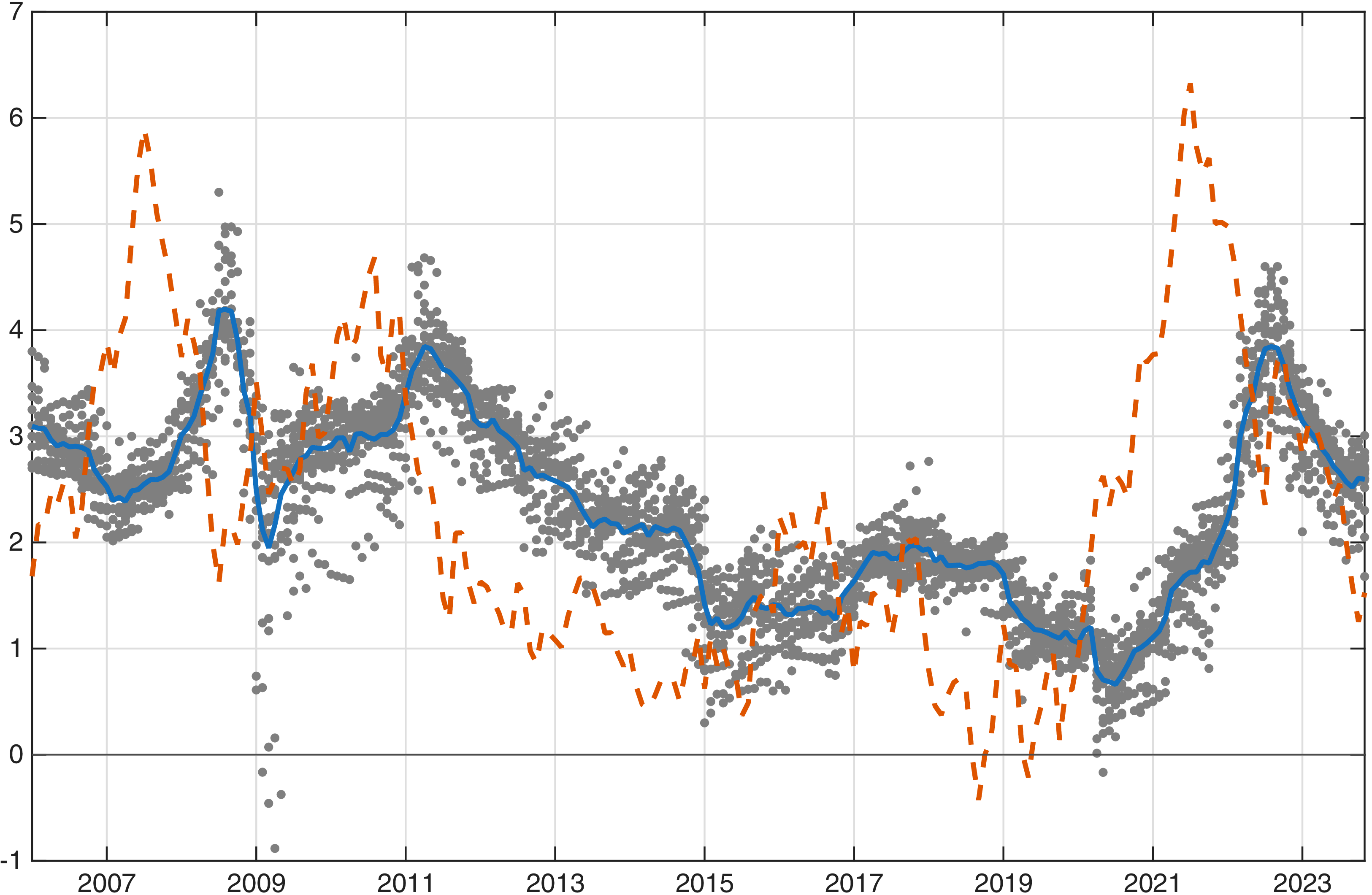
Figure 1 plots the individual one-year ahead inflation forecasts and the mean forecast across forecasters, along with realized inflation 12 months later. After a peak during the global financial crisis in 2008, the mean inflation forecast fell until the COVID-19 pandemic. The individual submissions to the Consensus Economics panel scatter around the mean forecast. Importantly, the extent of disagreement varies over the sample period. Forecasters disagreed the most in early 2009 with some expecting inflation to be around three percent, while others expecting deflation.
Inflation expectations from the Consensus Economics panel.
Notes: The figure shows the individual one-year ahead inflation forecasts from the Consensus Economics panel for Korea as well as the mean forecast (blue line) and the realized inflation rate in
 $t+12$
(orange line).

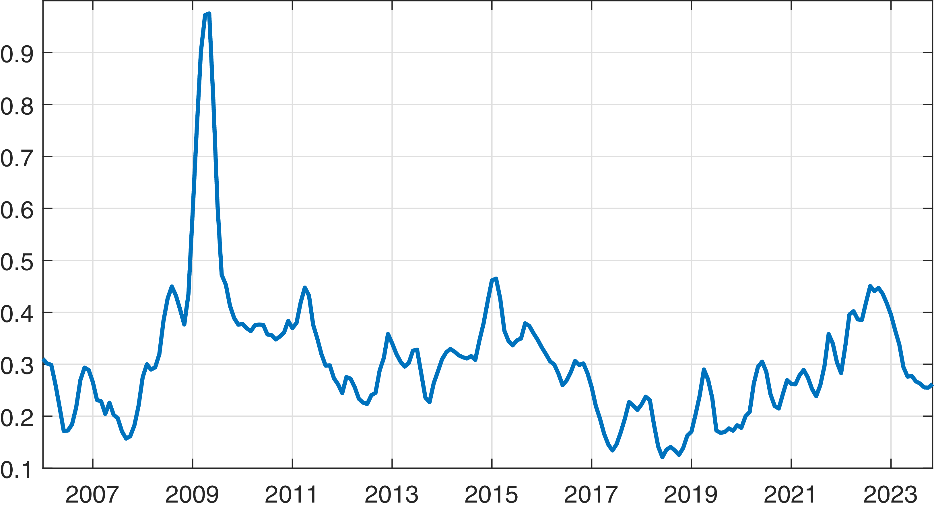
Figure 2 shows our baseline measure of disagreement, the cross-sectional standard deviation of forecasts. Disagreement was very high in 2009 and remained elevated until 2016, then fell and reached a minimum in 2018 before it increased again after 2020.
Inflation disagreement in the Consensus Economics panel.
Notes: The figure shows the cross-sectional standard deviation of inflation in the Consensus Economics panel.

3. Data and empirical model
In this section, we consider the local projections to investigate whether and how the level of inflation disagreement influences effectiveness of monetary policy transmission. We identify monetary policy shocks in Korea using the high-frequency identification scheme.
3.1. Local projections
We estimate local projections (Jordà, Reference Jordà2005)
 \begin{equation} y_{t+h}=\alpha _{h}+\beta _{h}\varepsilon _{t}+\gamma _{h}X_{t}^{\prime }+u_{t+h}, \end{equation}
for
 $h=0, 1, \ldots , H$
, where the monetary policy shock
 $\varepsilon _{t}$
at time
 $t$
drives the dependent variable at time
 $t+h$
. We explain the definition of policy shock in the next subsection. The key parameter of interest is
 $\beta _{h}$
, which measures the impact of the monetary policy shock. Plotting this parameter as a function of
 $h$
provides us with the impulse response function of the dependent variable to a monetary policy shock after
 $h$
periods. The vector
 $X_{t}$
contains control variables and the projection residuals are
 $u_{t+h}$
.
The monthly dependent variables are the unemployment rate, the year-on-year(y-o-y) percentage change of the index of Industrial Production, the y-o-y percentage change of the Consumer Price Index, the mean one-year ahead inflation expectation from Consensus Economics, the mean one-year ahead inflation expectation from the BOK Consumer SurveyFootnote 5 and the mean one-year ahead expectation of GDP growth from Consensus Economics.
We estimate the model with four lags of the dependent variable and the control variables. The vector of control variables includes lags of the current dependent variable
 $y_{t}$
, lags of the other dependent variables, the two-year U.S. interest rate, the (log) VIX index of implied volatility, the index of global economic conditions of Baumeister et al. (Reference Baumeister, Korobilis and Lee2022), the (log) global price index of all commodities and a dummy that is one between March and May 2020 and zero otherwise. This dummy captures the first three months of the COVID-19 pandemic. We estimate the model over the sample period from January 2006 to November 2023. Details of the data set are available in the Appendix B.
Thus far the model is able to trace the effect of monetary policy on the Korean economy independently from the extent of forecast disagreement. We now augment the model in order to allow the transmission of monetary policy to be dependent on the level of disagreement. Specifically, we adopt a smooth-transition local projection approach (Auerbach and Gorodnichenko, Reference Auerbach, Gorodnichenko, Auerbach and Gorodnichenko2013; Tenreyro and Thwaites, Reference Tenreyro and Thwaites2016) as follows
 \begin{eqnarray} y_{t+h} &=&F\big ( \widehat {dis}_{t-1}\big ) \left [ \alpha _{h}^{I}+\beta _{h}^{I}\varepsilon _{t}+\gamma _{h}^{I}X_{t}^{\prime }\right ] \\[4pt] &&+\big ( 1-F\big ( \widehat {dis}_{t-1}\big ) \big ) \left [ \alpha _{h}^{II}+\beta _{h}^{II}\varepsilon _{t}+\gamma _{h}^{II}X_{t}^{\prime }\right ] +u_{t+h}, \nonumber \end{eqnarray}
with a separate set of parameters in states I and II. If all parameters of the model are invariant to the state, the model collapses to the linear specification introduced before. Put differently, the linear model shown before is a special case of this mixture of two states with
 $F(.)=1$
. We are particularly interested in the estimates of
 $\beta _{h}^{I}$
and
 $\beta _{h}^{II}$
, i.e. the responses to policy shocks across the two states. The transition function
 $F\big ( \widehat {dis}_{t-1}\big )$
indicates the probability of being in the state I conditional on the level of disagreement,
 \begin{equation} F\big ( \widehat {dis}_{t-1}\big ) =\frac {\exp\!\big(\theta \widehat {dis}_{t-1}\big ) }{1+\exp \!\big(\theta \widehat {dis}_{t-1}\big )}, \end{equation}
where
 $\widehat {dis}_{t-1}$
is the standardized time series of the cross-sectional standard deviation of inflation forecasts or an alternative measure of disagreement in
 $t-1$
. We use the first lag of the state variable in order to avoid feedback from the policy surprise on the state variable. The transition function maps the disagreement about future inflation into the
 $[0,1]$
interval. The parameter
 $\theta$
determines the smoothness of the transition across states, where a lower
 $\theta$
implies a smoother shift between the states. We set
 $\theta =3$
, which is a standard value in the literature and implies an intermediate degree of smoothness.
3.2. Monetary policy shocks
The monetary policy shock should reflect unexpected changes in monetary conditions. We follow the literature on the high-frequency identification of policy shocks and use information from the market responses to BOK decisions in order to derive a monetary policy shock.Footnote 6 To the extent interest rates reflect expectations about future monetary policy, changes in interest rates on BOK meeting days should fully reflect the new information about monetary policy. As we do not have intraday data, we resort to the change in market interest rates between the day of the policy decision and the day before. Thus, the identifying assumption is that no information other than new information about monetary policy systematically drives the change in interest rates on meeting days.
Our preferred measures of the policy surprise,
 $surp_{t,d}$
, are either the change in the 12-month Korean Inter-bank Offered Rate (KORIBOR) or the change in the rate on three-month Certificates of Deposit (CD91), where
 $t$
and
 $d$
indicate the month and the day of the BOK decision. The BOK’s Monetary Policy Board, the policy-setting body, met monthly until 2017 and eight times per year thereafter. Thus, the policy shock used in the estimation of local projections,
 $\varepsilon _t$
, is either the surprise in a month with a meeting or zero in a month without a meeting, i.e.
 \begin{equation*} \varepsilon _{t}=\left \{ \begin{array}{c} surp_{t,d} \\ 0 \end{array} \begin{array}{l} \text{if BOK decision in month $t$} \\ \text{if no BOK decision in month $t$} \end{array} \right . \end{equation*}
Both interest rates reflect all information revealed on BOK meeting days. This includes not just information on the immediate change in short-term rates, but also on the path of monetary policy in the near future. The latter is an important part of monetary policy communication, but would not be reflected in an overnight rate. We are not claiming that the BOK uses the 12-month KORIBOR or the CD rate as an instrument of policy. Rather, we assume that all new information revealed on meeting days is best incorporated in either of these two rates.Footnote 7
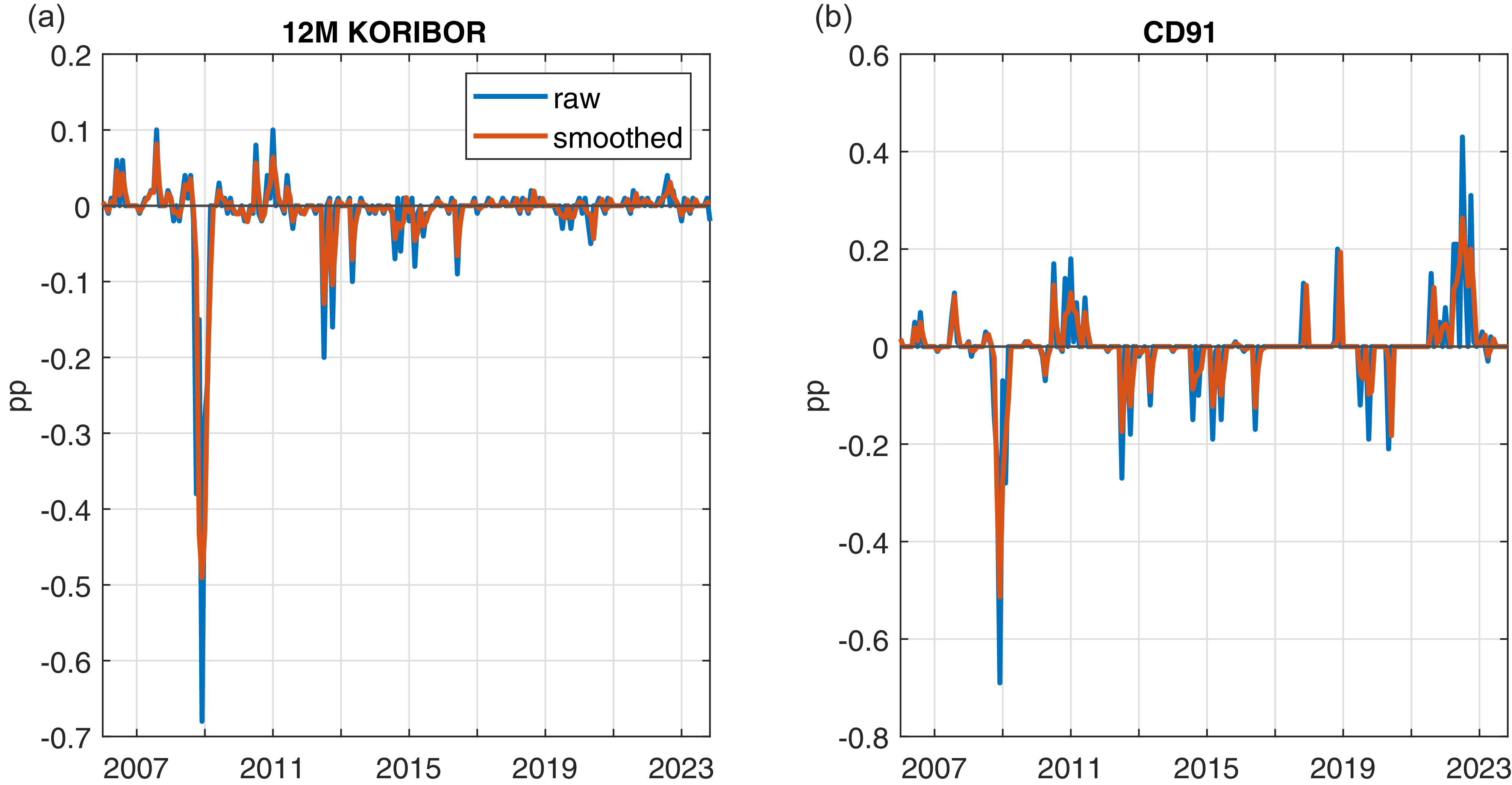
Figure 3 shows the resulting series of monetary policy shocks. The largest easing surprises occurred in 2008/09 around the global financial crisis. Between 2012 and 2015, the BOK also announced several interest rate steps which were interpreted by markets as unexpected easings of monetary conditions. The decision on July 12, 2012 implied a strong easing surprise when the BOK unexpectedly cut its benchmark rate by 25 basis points. The figure shows one notable difference between our two surprise series. The KORIBOR does not reflect the large tightening surprises in 2022/23, which are clearly reflected in the CD91 surprise. For this reason, we consider the CD91 surprise as our baseline monetary policy shock and use the KORIBOR surprise series and smoothed CD91 and KORIBOR surprises only to examine the robustness of our results.
Change in interest rates on BOK meeting days.
Notes: The figure shows
 $\varepsilon _t$
, i.e. the change in short-term interest rates on meeting days of the BOK’s Monetary Policy Board. The shock is zero in months without a BOK meeting. The left figure shows the change in the 12-month KORIBOR, and the right figure the change in the CD91 rate. Both figures also show the smoothed shock series in line with Gertler and Karadi (Reference Gertler and Karadi2015).

4. Empirical results
In this section, we present the impulse responses of inflation, inflation expectations, and other key macroeconomic variables to a monetary policy shock for both linear and state-dependent local projections. For state-dependent impulse responses, we condition the responses on the level of disagreement about inflation expectation.
4.1. Results from linear model
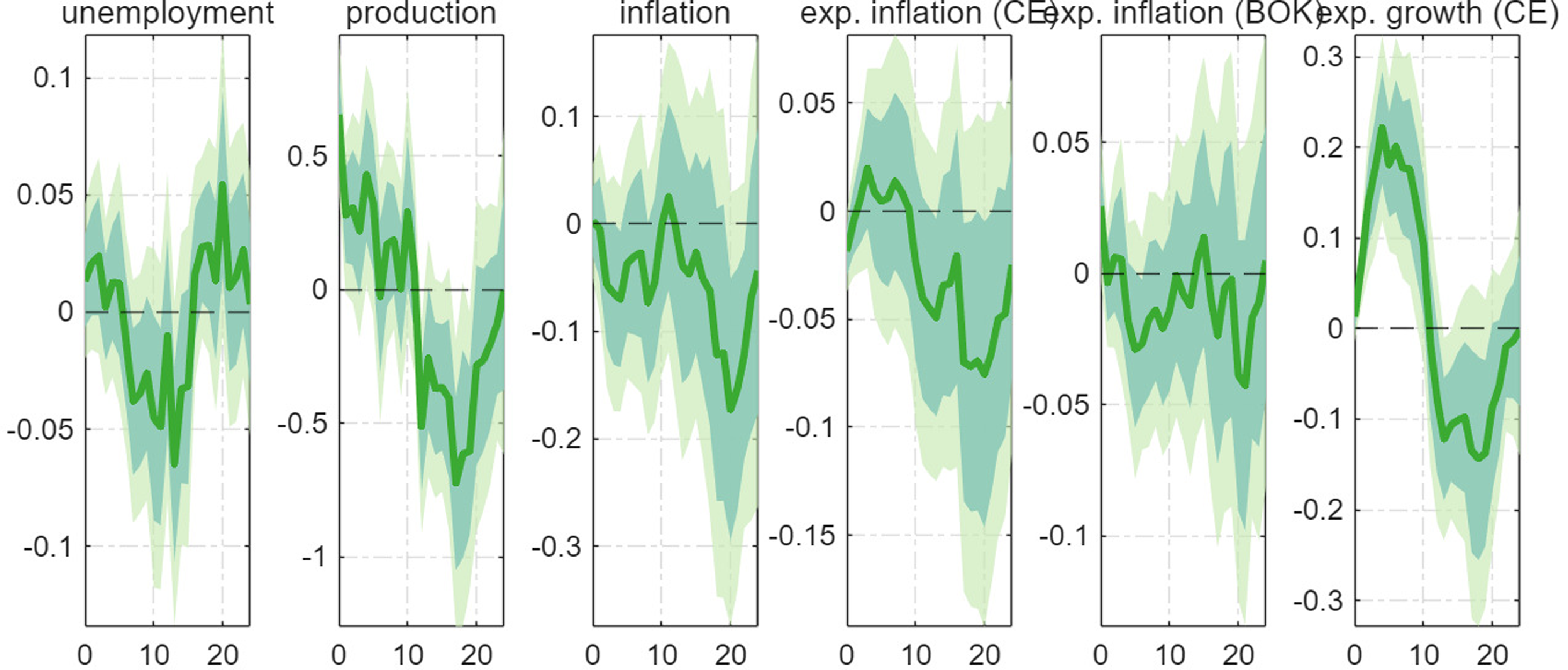
Figure 4 shows the results from the linear model based on equation (1). We plot the estimated coefficient
 $\beta _h$
as a function of the projection horizon
 $h$
. As the data is monthly, this corresponds to the responses of the endogenous variables
 $h$
months after the shock. We also show 68% and 90% confidence bands constructed from Driscoll and Kraay (Reference Driscoll and Kraay1998) standard errors. We scale the monetary policy shock such that the estimates reflect the impact of a shock ten basis points in size. After a surprise monetary tightening, unemployment falls. This effect, though small and borderline significant, is not in line with textbook logic which suggests a contraction of economic activity after a tightening. The growth rate of industrial production increases in the first couple of months after the shock, before it falls significantly. Forecasters expect high GDP growth following the shock, which is also counterintuitive. The responses of actual and expected inflation remain inconclusive.
Effect of monetary policy shock: linear model.
Notes: The figure shows the estimated
 $\beta _{h}$
coefficient as a function of
 $h$
as well as 68% and 90% confidence bands constructed from Driscoll and Kraay (Reference Driscoll and Kraay1998) standard errors. The shock is scaled such that the coefficient shows the impact of a shock of 10 basis points.

Overall, these responses are not in line with standard economic theories. One reason could be that the linear model shows us the average of two states of the world prevailing in the background: one state in which the signaling effect dominates and one in which the conventional logic dominates. This is why we now move on to study the effect of monetary policy depending on the level of disagreement among forecasters.
4.2. State-dependent impulse responses
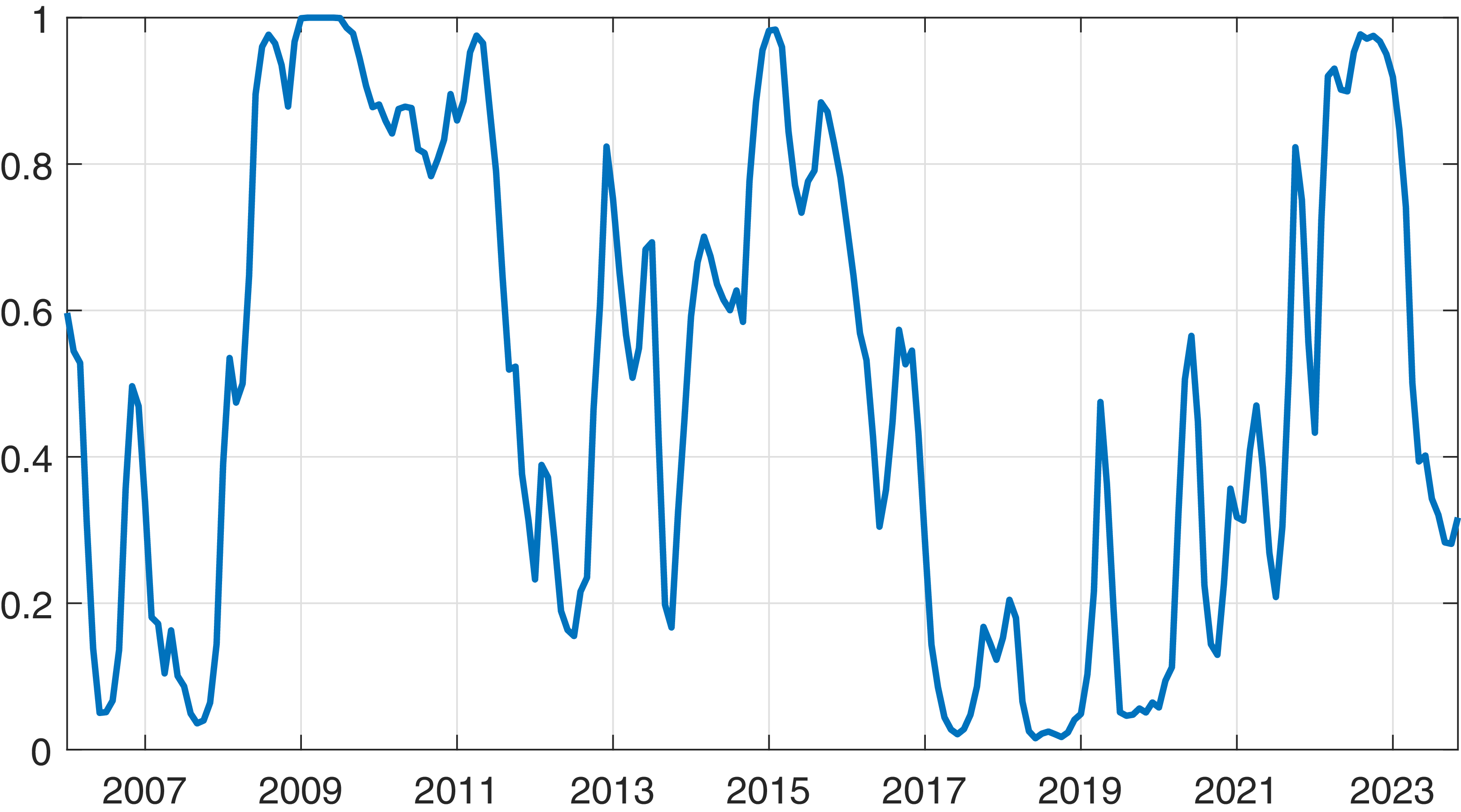
We now turn to the results of the smooth-transition model, i.e., the state-dependent responses to monetary policy. Figure 5 plots the transition function, i.e., the probability of state I, the high-disagreement state. Between 2008 and 2011 and between 2014 and 2017, the economy is clearly in a high-disagreement state. From 2017 until the start of the COVID-19 pandemic in early 2020, the economy is characterized by a low-disagreement state, before the model jumps back to state I.
Probability of being in high disagreement state.
Notes: The figure shows
 $F\left ( \widehat {dis}_{t-1}\right )$
, i.e. the probability of the high-disagreement state. Disagreement is measured by the standard deviation of one-year ahead inflation forecasts from Consensus Economics.

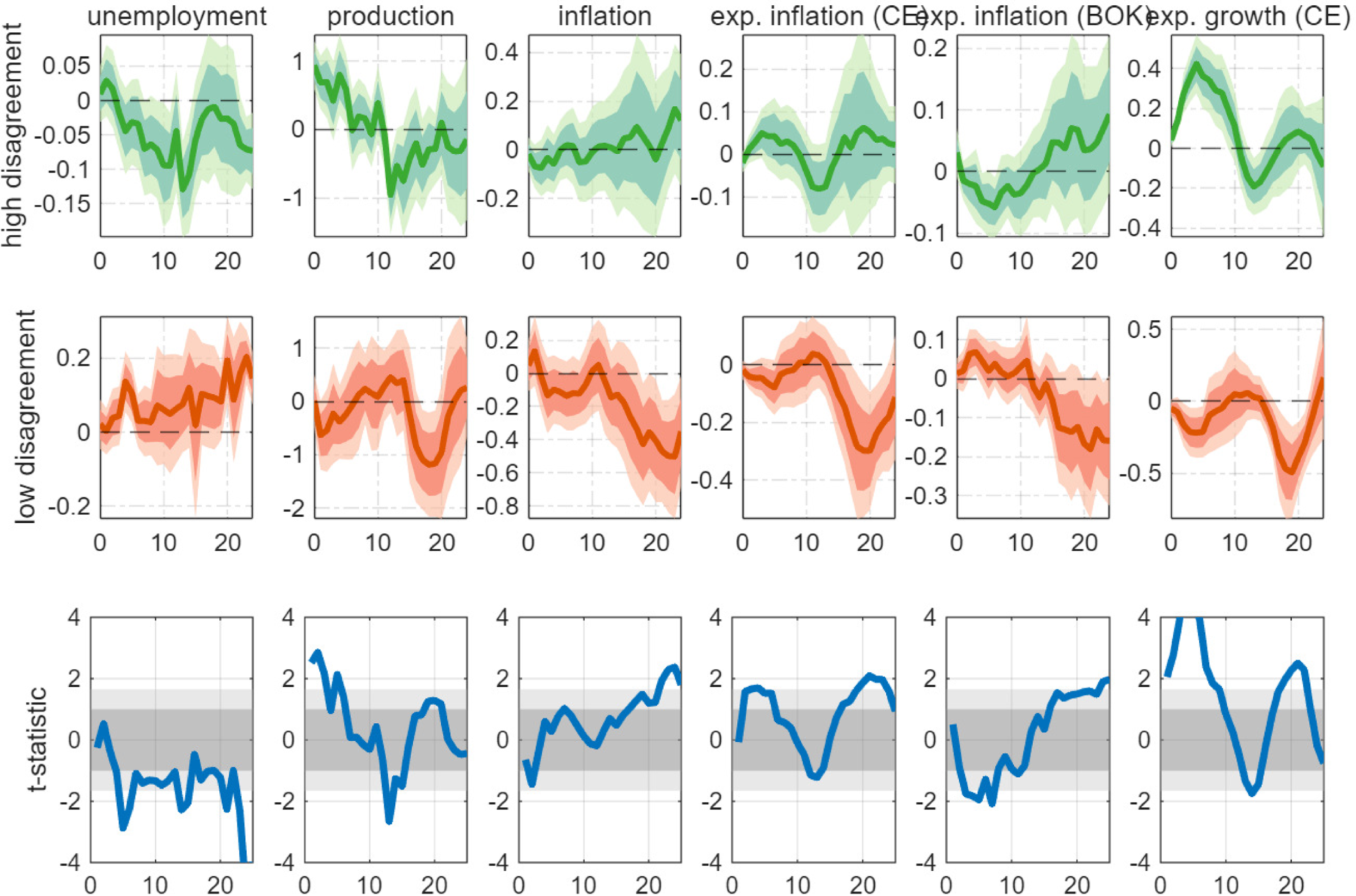
Based on this separation of regimes, Figure 6 plots the estimated coefficients
 $\beta _h^{I}$
and
 $\beta _h^{II}$
in equation (2) for the projection horizon
 $h$
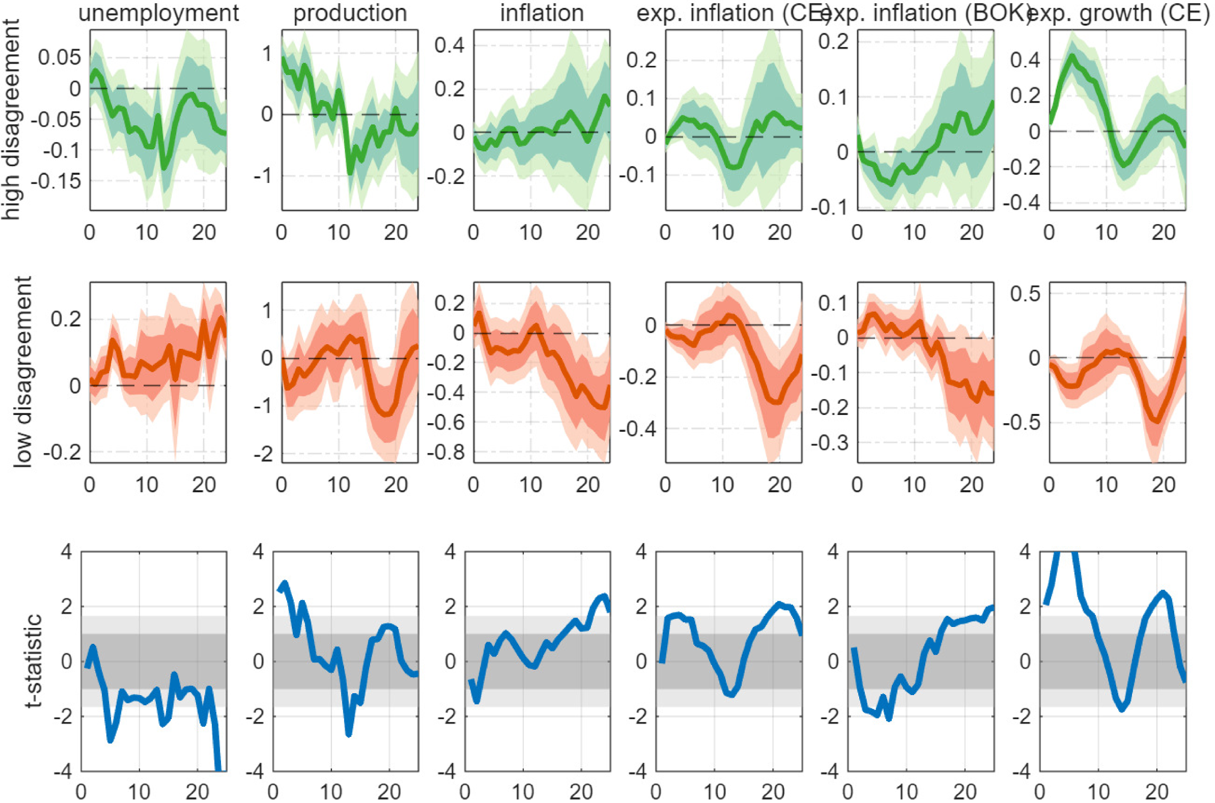
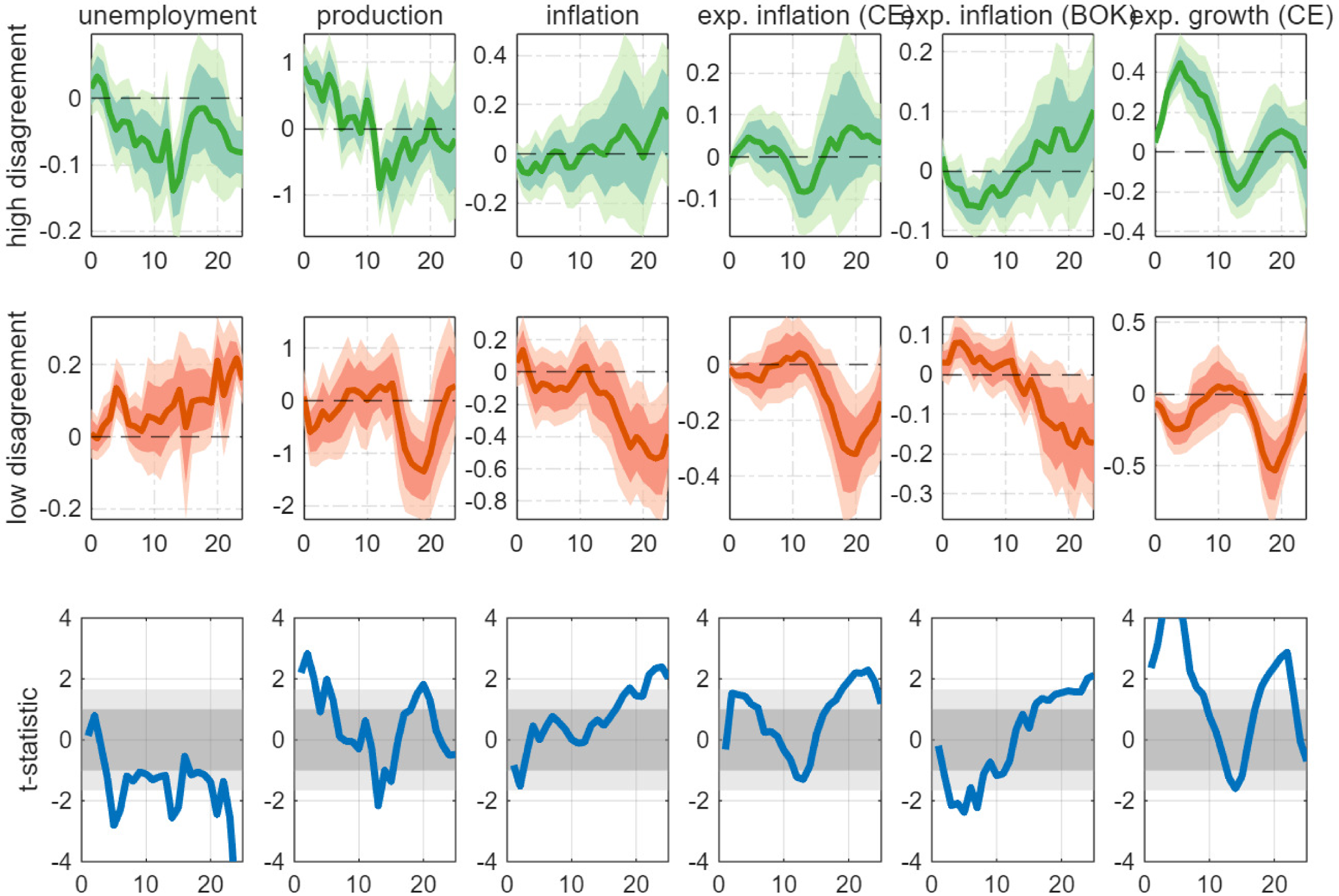
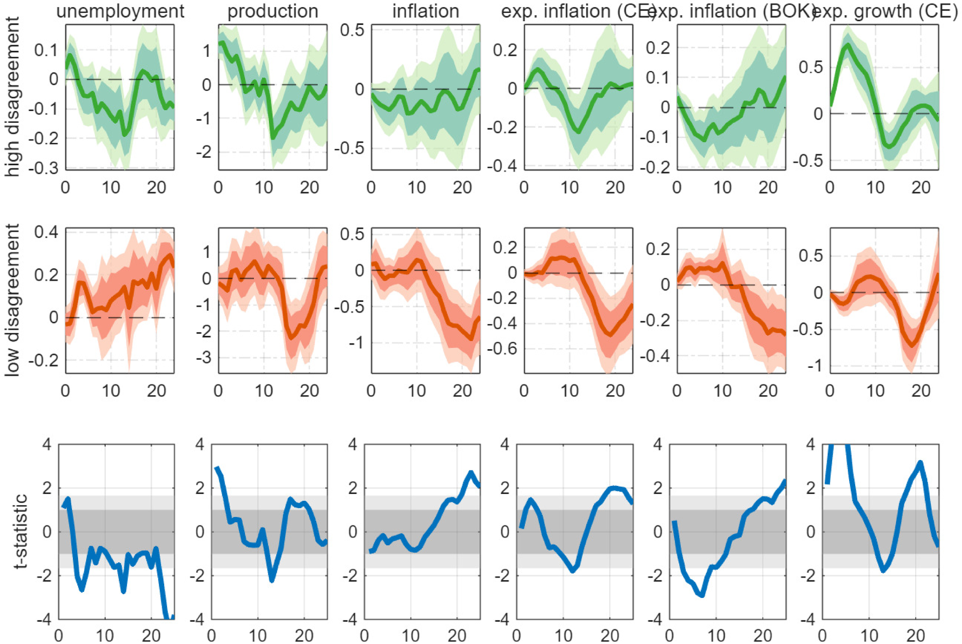
with 68% and 90% confidence bands. The figure reports the most important findings from the state-dependent model. If disagreement about future inflation is high, i.e., the economy is in state I, the responses of activity and inflation (expectations) remain insignificant or are at odds with standard economic theory. Unemployment falls after a contractionary policy shock and growth forecasts improve. The responses of inflation remain inconclusive.
Effect of monetary policy shock: state-dependent model.
Notes: The first two panels show the estimated
 $\beta _{h}$
coefficients in the high- and low-disagreement states as a function of
 $h$
as well as 68% and 90% confidence bands constructed from Driscoll and Kraay (Reference Driscoll and Kraay1998) standard errors. The shock is scaled such that the coefficients show the impact of a shock of 10 basis points. Disagreement is measured as the standard deviation across forecasters. The third panel shows the
 $t-$
statistic for the hypothesis of equal
 $\beta _{h}$
coefficients in the high- and low-disagreement states. The gray areas show critical values at the 68% and 90% confidence level.

The nature of the responses changes drastically if the economy is in a low-disagreement state. A policy tightening now causes a significant increase in unemployment, a drop in growth, a fall in actual inflation, a fall in expected inflation from Consensus Economics, and a drop in expected inflation from the BOK Consumer Survey. In addition, the mean forecast of one-year ahead GDP growth falls. The responses are quantitatively strong: a policy tightening of 10 basis points causes a fall in actual inflation of about 0.4 percentage points and a decline in expected inflation of about 0.2 to 0.3 percentage points in the long run. Hence, the responses in state II are fully in line with the standard economics textbook. This suggests that high levels of disagreement severely affect the nature of monetary policy transmission. After a transition to a low-disagreement state, the economy exhibits the expected responses to monetary policy shocks.
The third panel of Figure 6 shows the
 $t$
-statistic for the hypothesis of equal
 $\beta _{h}$
coefficients in the high- and low-disagreement states. The gray areas show critical values at the 68% and 90% confidence level. The responses of unemployment and expected growth are significantly different across the two states. Likewise, actual and expected (BOK) inflation fall in the low-disagreement state, which is significantly different from the responses in the high-disagreement state.
The results are consistent with the logic of sticky-price models under dispersed information of firms (Melosi, Reference Melosi2017; Falck et al., Reference Falck, Hoffmann and Hürtgen2021). Under low disagreement, the conventional transmission channel of monetary policy dominates the signaling channel. Hence, inflation falls. If disagreement is high, the surprise tightening serves as a signal for price-setters that the state of the economy is better than expected. Hence, the signaling channel dominates the standard transmission channel. As a result, inflation and expected inflation increase or remain insensitive to monetary policy in state I.
We conduct a battery of checks to demonstrate the robustness of the baseline finding. First, for alternative inflation disagreement measures, we consider the interquartile range of forecasts, the spread between the maximum and the minimum forecast submitted each month as well as non-smoothed standard deviation across forecasts. Second, to mitigate concerns about model misspecification, we additionally consider the empirical cumulative distribution function of the state variable following Born et al. (Reference Born, Müller and Pfeifer2020), which does not parameterize the transition function (3) in a smooth-transition local projection model. Third, we use KORIBOR surprise series and smoothed CD91 and KORIBOR shock series as alternative monetary policy shocks. Our baseline results are robust to alternatives to inflation disagreement measures, specifications of transition function, and monetary policy surprises, respectively. A collection of robustness checks related to the specification of empirical analyses is available in the Appendix C.
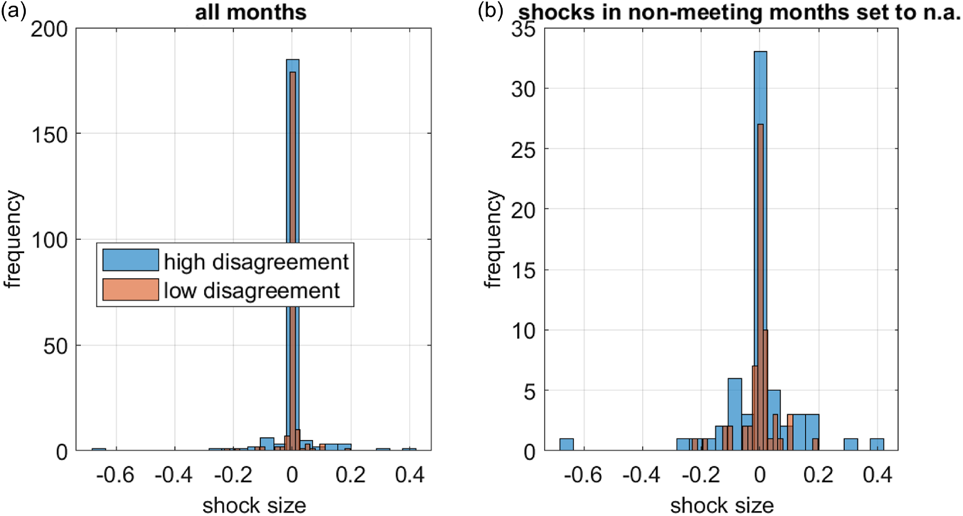
Lastly, we plot the distribution of monetary policy shocks in high- and low-disagreement states. Tightening and expansionary monetary policy shocks are largely evenly distributed across the two states, implying that our results are not primarily driven by an asymmetric distribution of tightening and expansionary monetary policy shocks across disagreement states and their asymmetric transmission effects. We provide further explanation in the Appendix C.4.
5. Extended experiments
Our empirical model allows the effectiveness of monetary policy shocks to be dependent on the level of disagreement about future inflation. In this section, we investigate the robustness of our results by also allowing shocks to interact with the level of monetary policy uncertainty, the changing nature of the BOK’s inflation target, and the level of disagreement about expectations of other variables in Consensus Economics.
5.1. Disagreement vs uncertainty
The disagreement across forecasts and the uncertainty perceived by forecasters describe different dimensions of surveys. Nevertheless, the literature (e.g. Bachmann et al. (Reference Bachmann, Elstner and Sims2013)) often uses measures of disagreement and uncertainty as close substitutes. In fact, both are typically highly correlated. Thus, in this section, we explicitly consider monetary policy uncertainty in the model.
Cho and Kim (Reference Cho and Kim2023) construct an index of economic policy uncertainty for Korea based on an analysis of the reporting about economic policy in 13 major Korean newspapers and a pre-specified dictionary of keywords related to economic policy uncertainty. The authors also provide a disaggregation of this index into different branches of policy, among them an index of monetary policy uncertainty. This categorical index is based on (the Korean translation of) expressions such as “monetary policy,” “inflation target,” “BOK” or “central bank” together with words such as “uncertain,” “uncertainty” or “concern.”
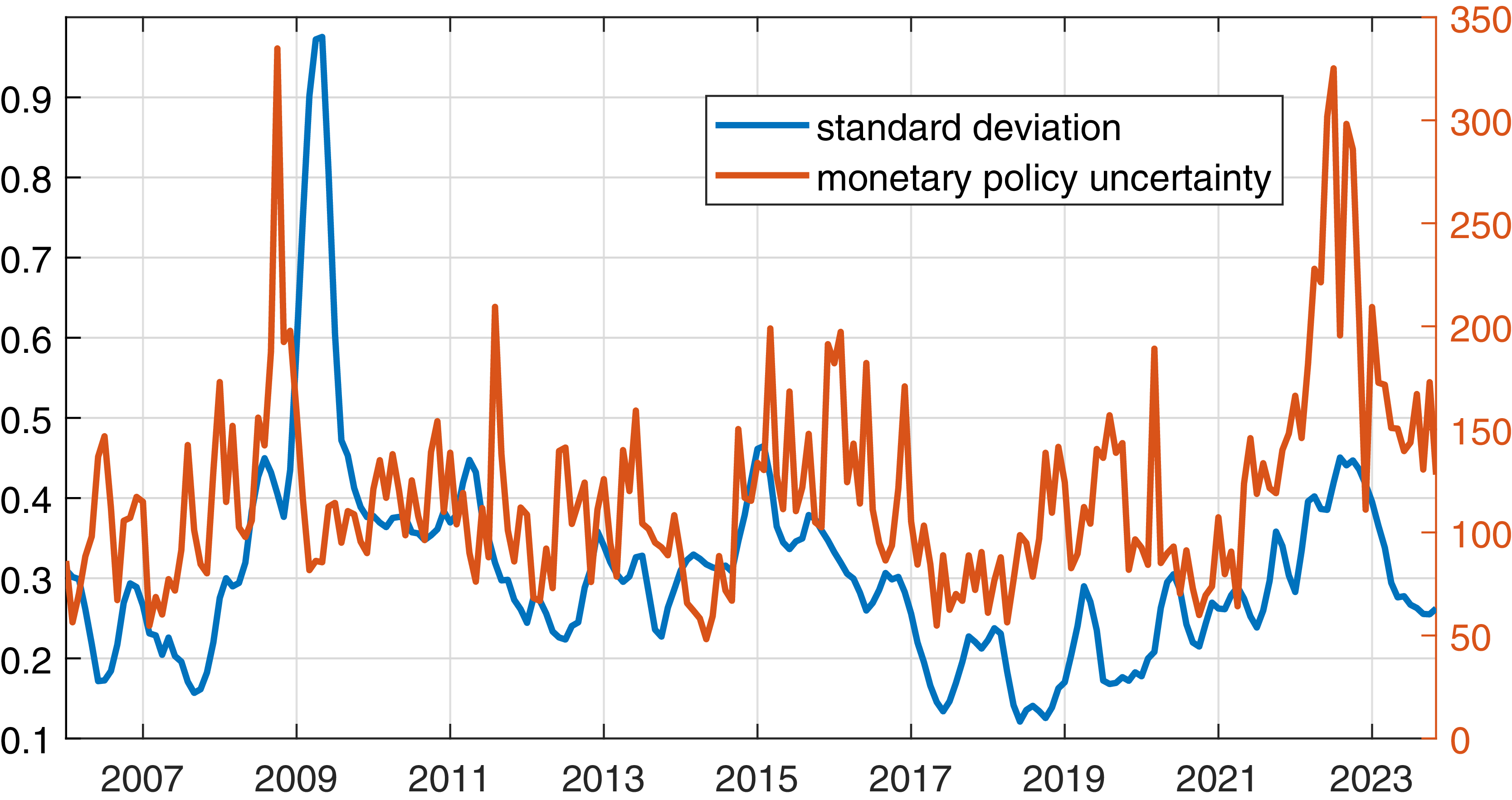
Figure 7 shows this index against the time series of forecast disagreement. Both series increased in 2008 during the global financial crisis, around 2015, and during the most recent tightening period. Interestingly, monetary policy uncertainty increased in 2020, when the COVID-19 pandemic hit, while forecast disagreement remained moderate.
Inflation disagreement vs monetary policy uncertainty.
Notes: The figure shows the disagreement about inflation (left axis) as measured by the standard deviation across forecasters and the newspaper-based measure of monetary policy uncertainty (right axis) of Cho and Kim (Reference Cho and Kim2023).

Since our measure of forecast disagreement is correlated with uncertainty, we examine whether the state-dependent effects of monetary policy survive if we control for monetary policy uncertainty. Specifically, we augment the model with an interaction between the policy shock and the monetary policy uncertainty as follows
 \begin{eqnarray} y_{t+h} &=&F\left ( \widehat {dis}_{t-1}\right ) \left [ \alpha _{h}^{I}+\beta _{h}^{I}\varepsilon _{t}+\gamma _{h}^{I}X_{t}^{\prime }+\delta _{h}^{I}(mpu_t \times \varepsilon _{t})\right ] \\ &&+\left ( 1-F\left ( \widehat {dis}_{t-1}\right ) \right ) \left [ \alpha _{h}^{II}+\beta _{h}^{II}\varepsilon _{t}+\gamma _{h}^{II}X_{t}^{\prime }+\delta _{h}^{II}(mpu_t \times \varepsilon _{t})\right ] +u_{t+h}, \nonumber \end{eqnarray}
where the coefficients
 $\delta _{h}^{I}$
and
 $\delta _{h}^{II}$
capture the effect of monetary policy uncertainty on the transmission and
 $mpu_t$
is the level of uncertainty from Cho and Kim (Reference Cho and Kim2023).Footnote
8
The estimates of our parameters of interest,
 $\beta _{h}^{I}$
and
 $\beta _{h}^{II}$
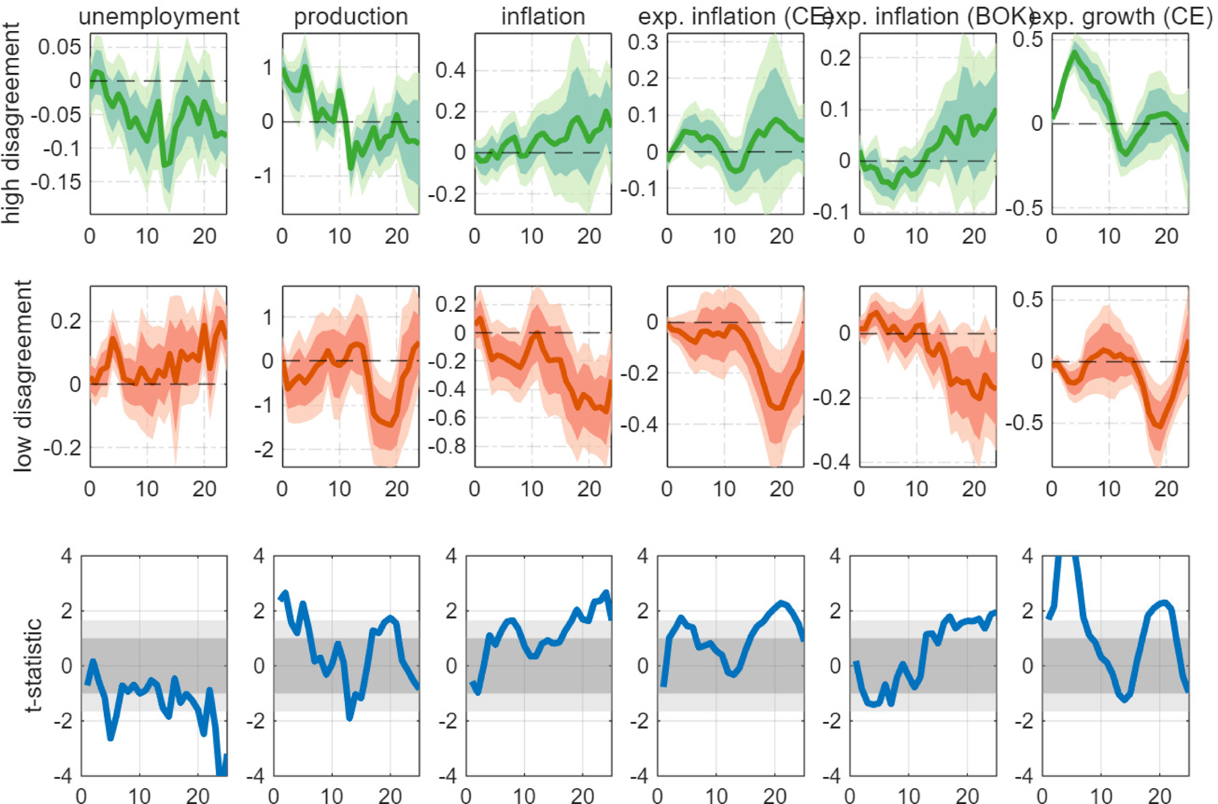
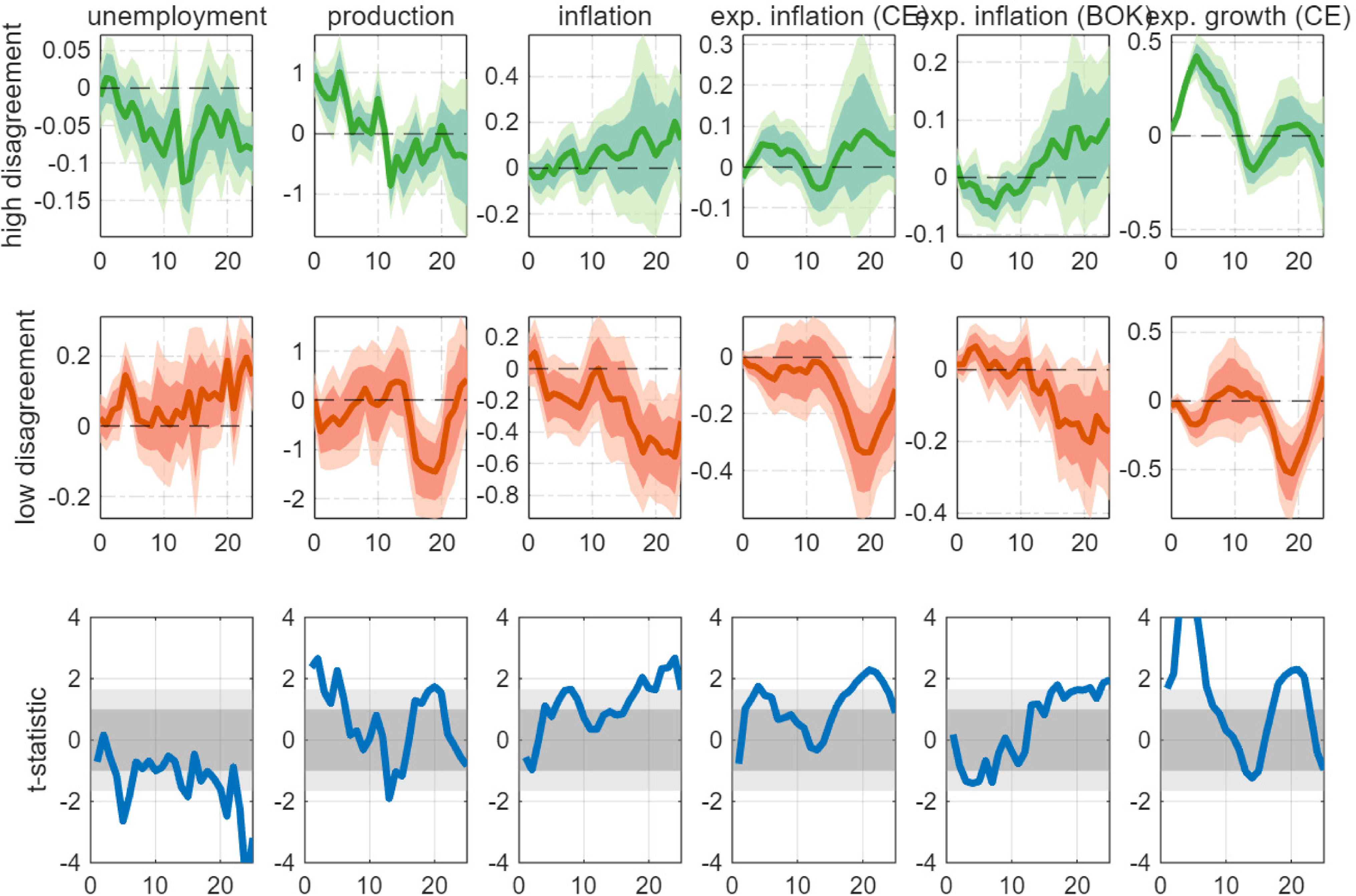
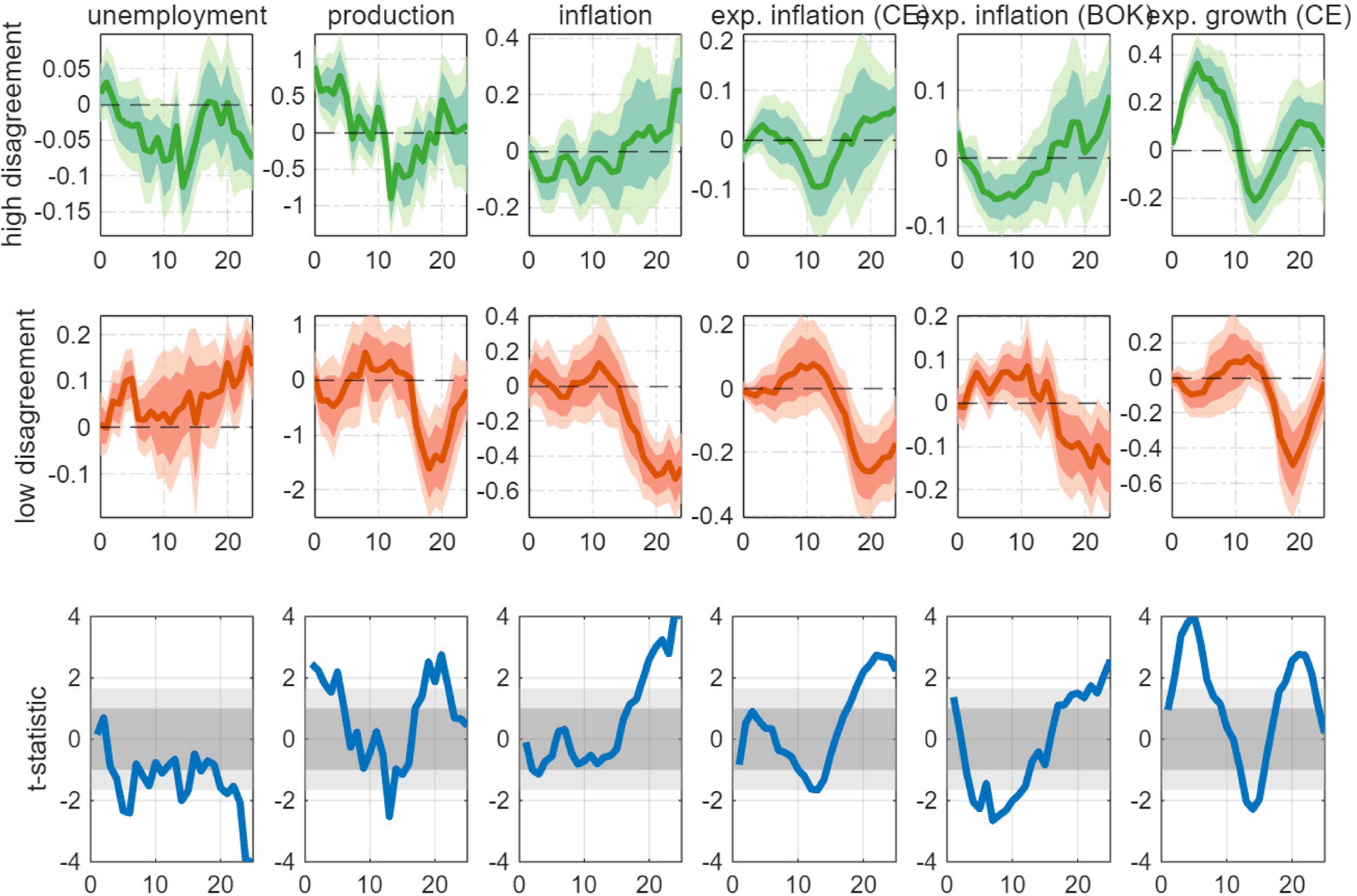
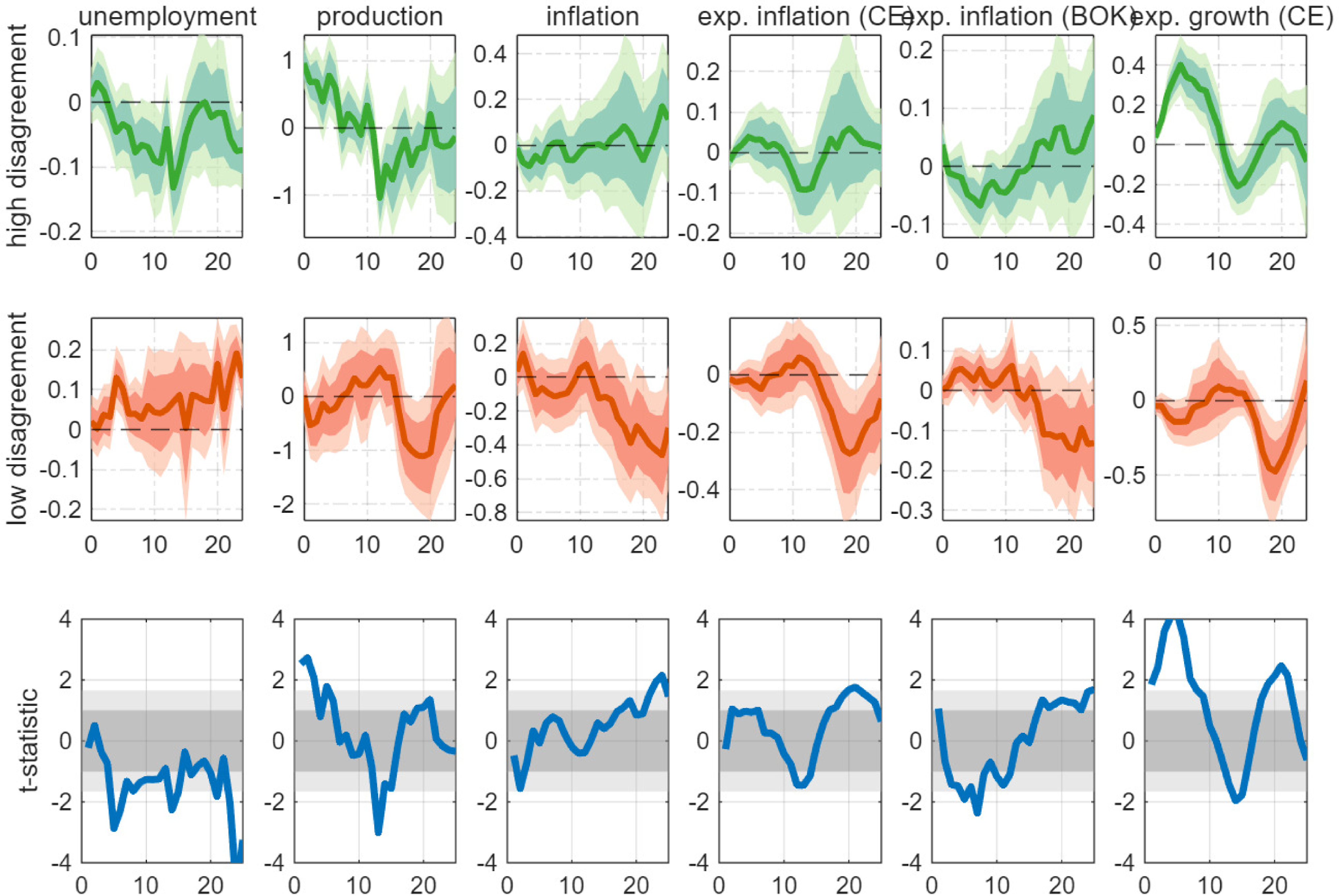
, are shown in Figure 8. We see that the findings from the baseline model survive. If disagreement is high, real activity improves after a tightening. This is reflected in a fall in unemployment, an increase in production, and a strong increase in expected future growth. The responses of the inflation rates remain inconclusive. However, if disagreement is low, all responses have the expected negative sign, with real activity contracting and inflation falling. These responses correspond to the findings from our baseline model and suggest that the state-dependent nature of impulse responses reflects the specific evolution of disagreement about expected inflation rather than the comovement with monetary policy uncertainty.
Effect of monetary policy shock: interaction with policy uncertainty.
Notes: The first two panels show the estimated
 $\beta _{h}$
coefficients in the high- and low-disagreement states as a function of
 $h$
as well as 68% and 90% confidence bands constructed from Driscoll and Kraay (Reference Driscoll and Kraay1998) standard errors. The shock is scaled such that the coefficients show the impact of a shock of 10 basis points. Disagreement is measured as the standard deviation across forecasters. The third panel shows the
 $t-$
statistic for the hypothesis of equal
 $\beta _{h}$
coefficients in the high- and low-disagreement states. The gray areas show critical values at the 68% and 90% confidence level.

5.2. The BOK’s evolving inflation target type
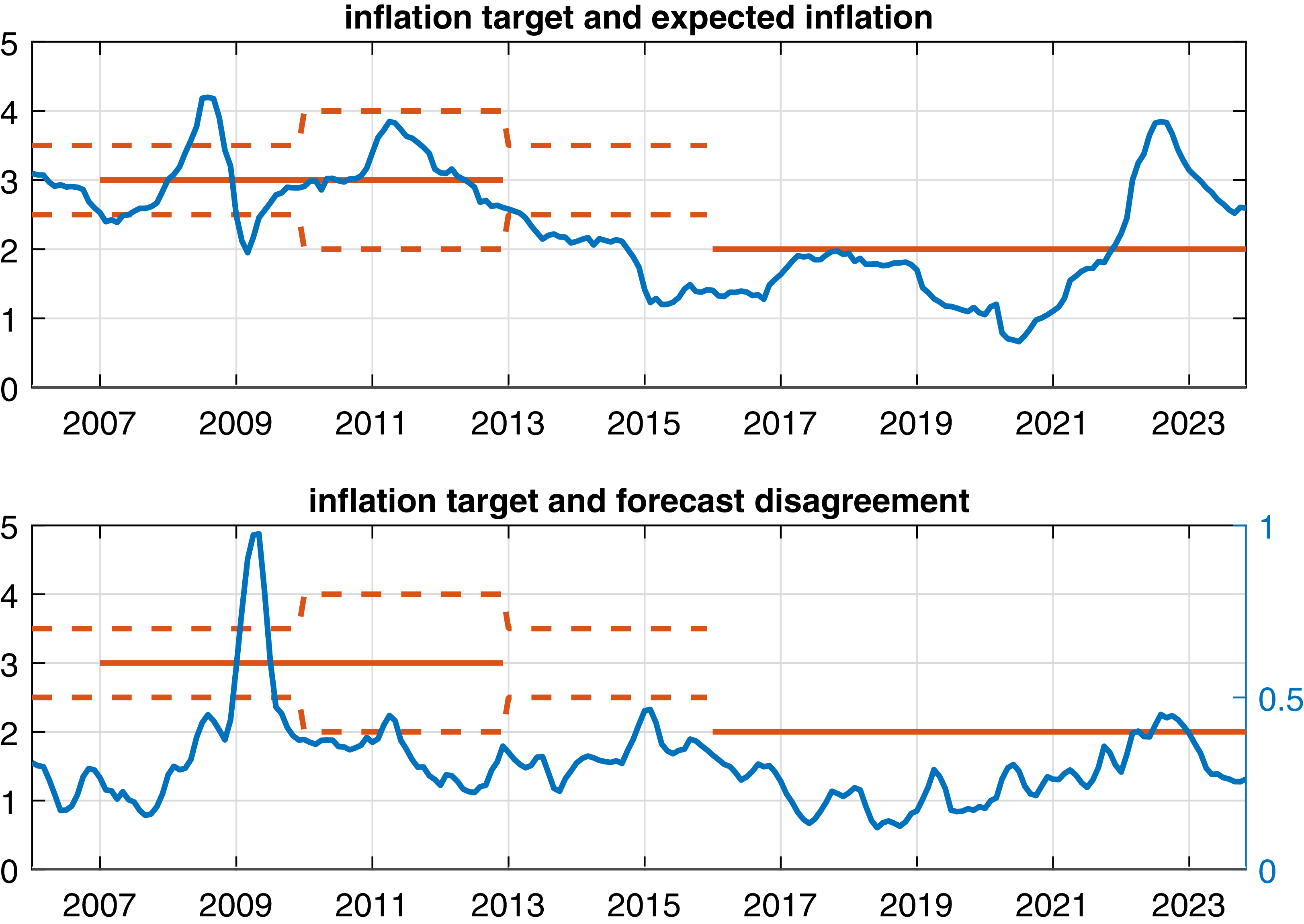
We attempt to understand whether the extent of inflation disagreement reflects the evolution of the BOK’s inflation target in this section. Until 2013, the BOK maintained a target range for inflation between 2% and 4% with a midpoint of 3%. Starting in January 2013, the range was narrowed to 2.5–3.5% without an explicit midpoint. Finally, the BOK switched to a point target for inflation of 2% in 2016. As narrowing the target range and eventually abolishing the range for a point target changes market expectations, it should also reduce the disagreement among forecasters. Figure 9 plots the evolution of the BOK’s inflation target against the mean forecast and the standard deviation across forecasters.Footnote 9
The evolution of the BOK’s inflation target.
Notes: The figure shows the evolution of the BOK’s inflation target as well as the mean forecast (first panel) and the standard deviation (second panel) of forecasts from the Consensus Economics panel. The latter variable is measured on the right axis. The dashed lines highlight the upper and lower bounds of the BOK’s target range. The solid lines show the midpoint and the point target, respectively.

It is possible that the switch from a target range to a (lower) point target in 2016 coincides with a lower mean forecast for inflation. However, our measure of disagreement should be independent of the change in the level of the inflation target and should only reflect the switching from a target range to a point target. The figure does indeed suggest a lower level of forecast disagreement after the institutional change, at least for the years between 2016 and 2020.Footnote 10 This coincidence makes it possible that the state-dependent effects of monetary policy uncovered in this paper are due to the changed type of inflation targeting in Korea rather than fluctuations in disagreement.
However, we show that the state-dependance does indeed result from changes in disagreement rather than an adjustment of the design of the inflation target. We define a dummy variable that takes the value of one until December 2015 and the value of zero after that date. Hence, the dummy picks up the change from a target range to a point target effective January 2016. We replace the interaction term in equation (4) with an interaction between the binary dummy,
 $D^{target}$
, and the monetary policy shock
 $\varepsilon _{t}$
. Hence, the model becomes
 \begin{eqnarray*} y_{t+h} &=&F\left ( \widehat {dis}_{t-1}\right ) \left [ \alpha _{h}^{I}+\beta _{h}^{I}\varepsilon _{t}+\gamma _{h}^{I}X_{t}^{\prime }+\delta _{h}^{I}(D^{target} \times \varepsilon _{t})\right ] \\ &&+\left ( 1-F\left ( \widehat {dis}_{t-1}\right ) \right ) \left [ \alpha _{h}^{II}+\beta _{h}^{II}\varepsilon _{t}+\gamma _{h}^{II}X_{t}^{\prime }+\delta _{h}^{II}(D^{target} \times \varepsilon _{t})\right ] +u_{t+h}, \end{eqnarray*}
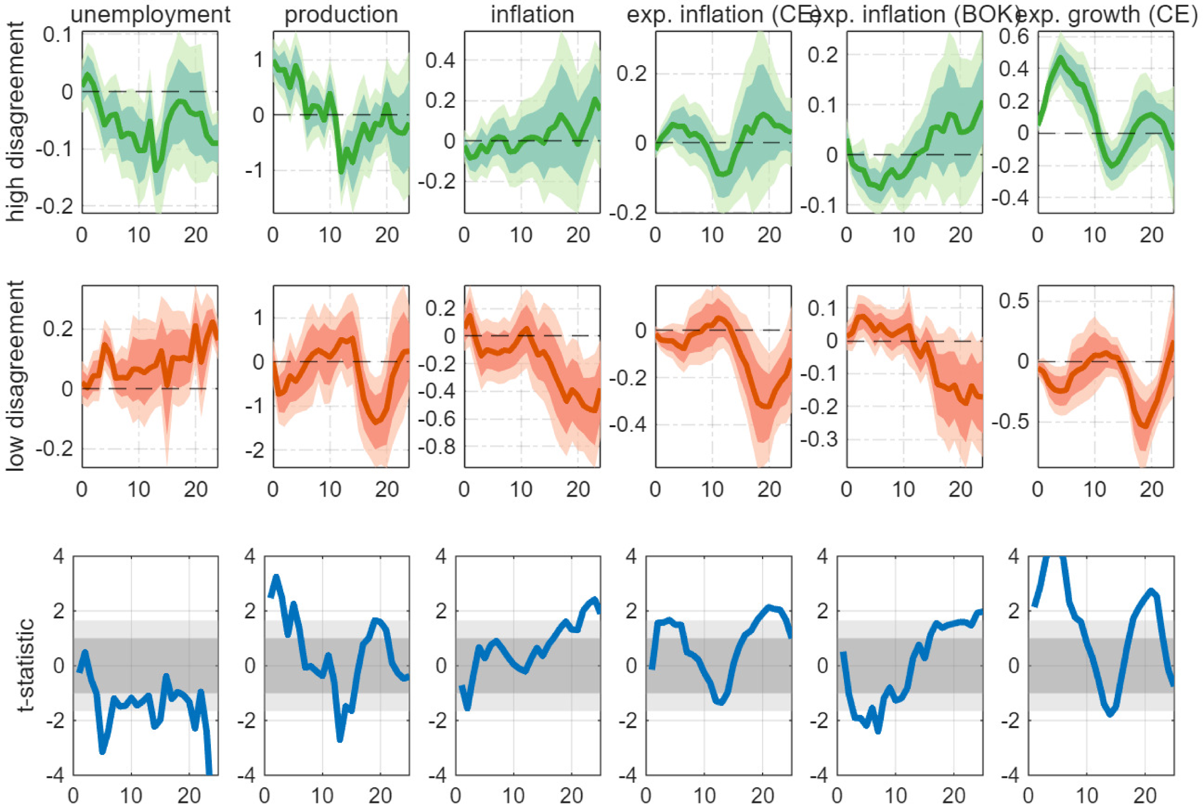
Monetary policy impulses can now affect the economy differently under the old and the new design of the inflation target, respectively, while we still allow for state-dependent effects with respect to inflation disagreement. The estimated coefficients are reported in Figure 10. The responses are either insignificant or have the wrong sign if disagreement is high. Hence, accounting for the changed type of the inflation target does not change the results discussed before.
Effect of monetary policy shock: interaction with the changing inflation target.
Notes: The first two panels show the estimated
 $\beta _{h}$
coefficients as a function of
 $h$
as well as 68 and 90% confidence bands constructed from Driscoll and Kraay (Reference Driscoll and Kraay1998) standard errors. The shock is scaled such that the coefficients show the impact of a shock of 10 basis points. Disagreement is measured as the standard deviation across forecasters. The third panel shows the
 $t$
-statistic for the hypothesis of equal
 $\beta _{h}$
coefficients in the high- and low-disagreement states. The gray areas show critical values at the 68% and 90% confidence level.

Therefore, we can conclude that our main findings reflect more than just a change in inflation target type. The disagreement among forecasters certainly affects the monetary transmission mechanism above and beyond the adjustment of the inflation target.
5.3. Disagreement about future growth and interest rates
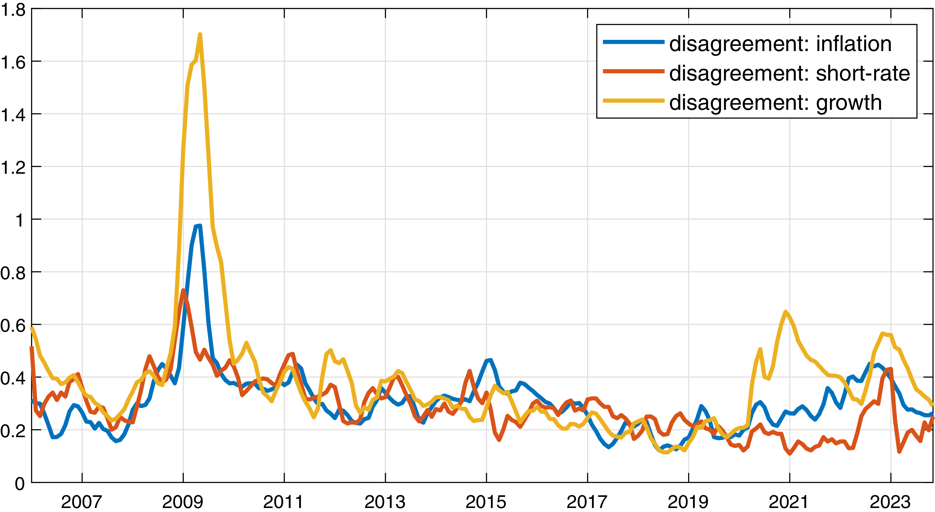
The Consensus Economics panel does not only include forecasts for inflation but also forecasts for GDP growth, the short-term interest rate, and the long-term interest rate. In the previous sections, the disagreement among forecasters about future inflation took center stage. We now shed light on disagreement about GDP growth and the short-term interest rate.Footnote 11 In particular, we now investigate whether disagreement about the remaining variables affects the role of inflation disagreement. Figure 11 shows the three series of forecast disagreement over the sample period. Interestingly, disagreement about real GDP peaked in 2009 in the wake of the global financial crisis and in 2020 during the COVID-19 pandemic. In both episodes, inflation disagreement increases less than disagreement about economic growth.
Disagreement about inflation, growth and the short-term interest rate.
Notes: The figure shows the (backward-looking) three-month moving average of disagreement about one-year ahead inflation, GDP growth, and the short-term interest rate as measured by the standard deviation across forecasters in the Consensus Economics panel.

We modify the regression specification in equation (4) by replacing the interaction of the policy shock with monetary policy uncertainty with the interaction with either disagreement about expected economic growth or expected short-term interest rates. Thus, we allow for policy shocks to be transmitted more or less strongly to the economy as a function of disagreement with respect to growth or short-term interest rate, while the state-dependance with respect to inflation disagreement remains in place.
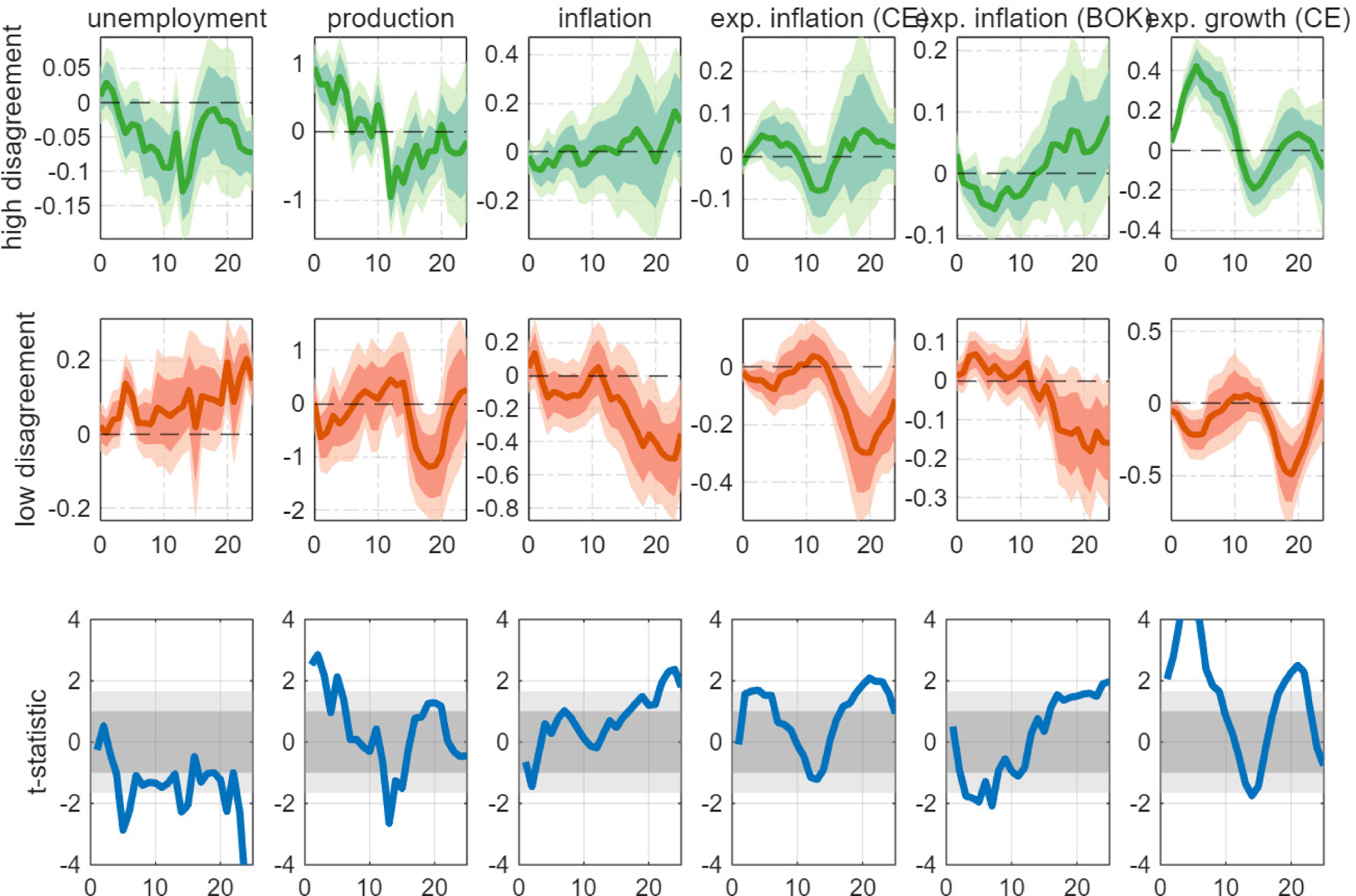
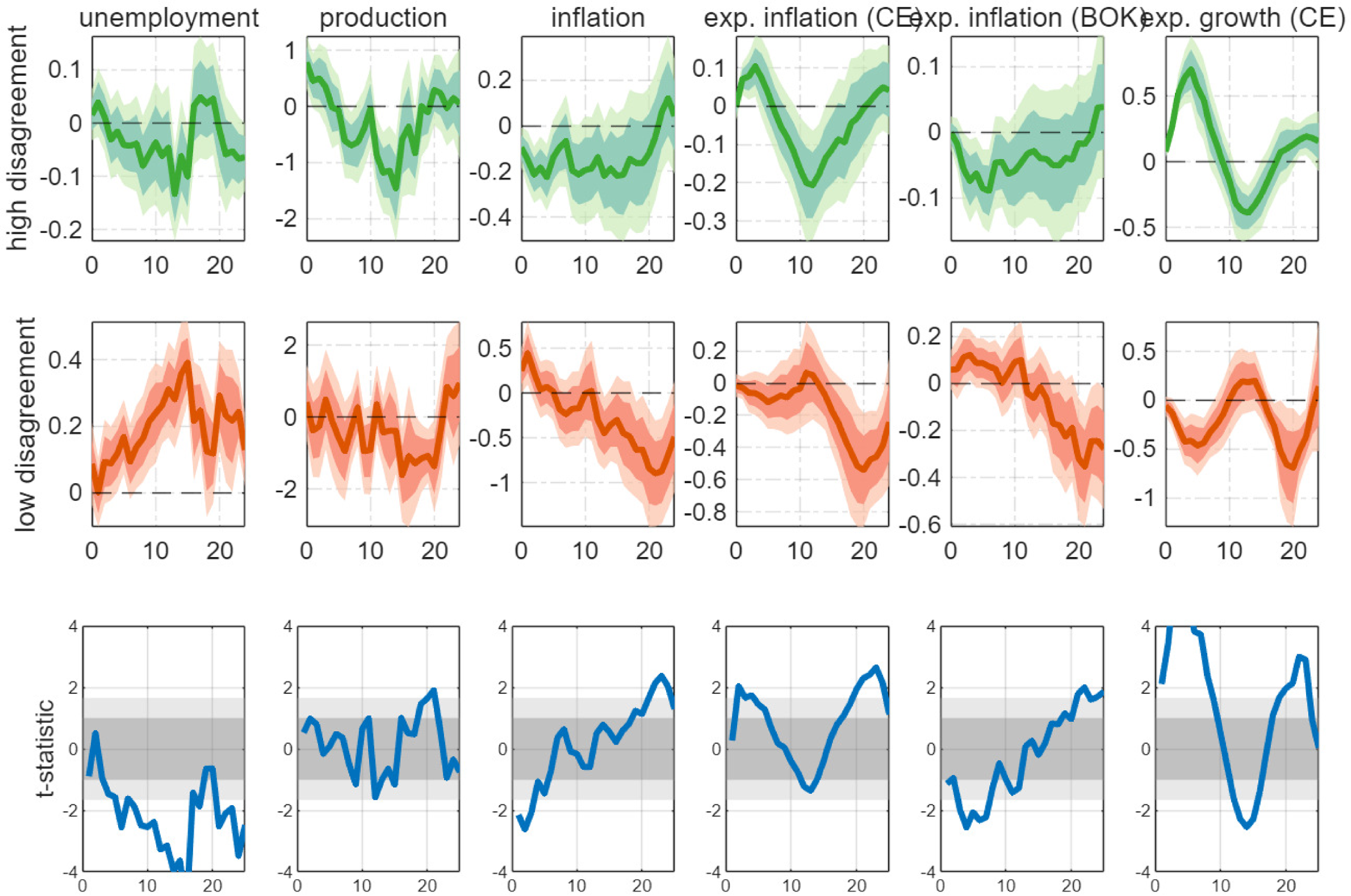
The results from the smooth-transition model interacted with GDP disagreement are shown in Figure 12. Our main findings remain unchanged. We find that a policy tightening increases unemployment, dampens production and reduces inflation in the low-disagreement state, but not in the high-disagreement state. Hence, including an interaction with disagreement about future growth does not overturn our main results.
Effect of monetary policy shock: interaction with disagreement about growth.
Notes: The first two panels show the estimated
 $\beta _{h}$
coefficients in the high- and low-disagreement states as a function of
 $h$
as well as 68% and 90% confidence bands constructed from Driscoll and Kraay (Reference Driscoll and Kraay1998) standard errors. The shock is scaled such that the coefficients show the impact of a shock of 10 basis points. Disagreement is measured as the standard deviation across forecasters. The third panel shows the
 $t-$
statistic for the hypothesis of equal
 $\beta _{h}$
coefficients in the high- and low-disagreement states. The gray areas show critical values at the 68% and 90% confidence level.

The same holds if we include an interaction between the policy shock and the disagreement about future short-term interest rates, as shown in Figure 13. Under high inflation disagreement, the responses remain insignificant or have the wrong sign, while the responses are in line with economic theory if inflation disagreement is low. Again, accounting for short-rate disagreement does not alter our findings.
Effect of monetary policy shock: interaction with disagreement about short-term interest rate.
Notes: The first two panels show the estimated
 $\beta _{h}$
coefficients in the high- and low-disagreement states as a function of
 $h$
as well as 68% and 90% confidence bands constructed from Driscoll and Kraay (Reference Driscoll and Kraay1998) standard errors. The shock is scaled such that the coefficients show the impact of a shock of 10 basis points. Disagreement is measured as the standard deviation across forecasters. The third panel shows the
 $t-$
statistic for the hypothesis of equal
 $\beta _{h}$
coefficients in the high- and low-disagreement states. The gray areas show critical values at the 68% and 90% confidence level.

6. Conclusions
Professional forecasters disagree about future inflation. This observation holds for advanced economies as well as emerging market economies. In this paper, we study the implications of forecast dispersion on the transmission of monetary policy in the case of Korea, transitioning from an emerging to an advanced economy. Based on a state-dependent model, we show that the effectiveness of monetary policy is significantly reduced if disagreement about inflation is high. In contrast, we document textbook-like effects of monetary policy under a low level of disagreement. Our findings suggest that the inflation-targeting regime in Korea shares an important property with monetary policy in advanced economies, such as the USA and the UK: the transmission of monetary policy shocks is affected by the level of forecast disagreement. We also show that the influence of disagreement is not a mere reflection of uncertainty about monetary policy or the change in the inflation-targeting type from range to point target adopted by the BOK.
Our findings also provide noteworthy policy implications on central banks’ communication. A high dispersion of inflation expectations can hamper monetary transmission. Thus, it is important not only to anchor the inflation expectations but also to reduce the dispersion over inflation expectations. Therefore, to reduce disagreement and, hence, to align individual forecasts, the BOK should enhance its communication with market participants and the wider public.
Acknowledgements
We are grateful for feedback from an anonymous reviewer of this journal, seminar participants at the Bank of Korea and the BI-ADBI-ADB-APAEA joint workshop as well as our discussants Hyundo Joo, Sangyup Choi, and Nuobu Renzhi. We also thank David Finck for helpful discussions and for sharing his local projections toolbox.
Appendix A. Details on the Consensus Economics panel
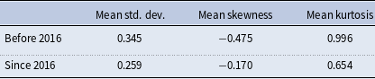
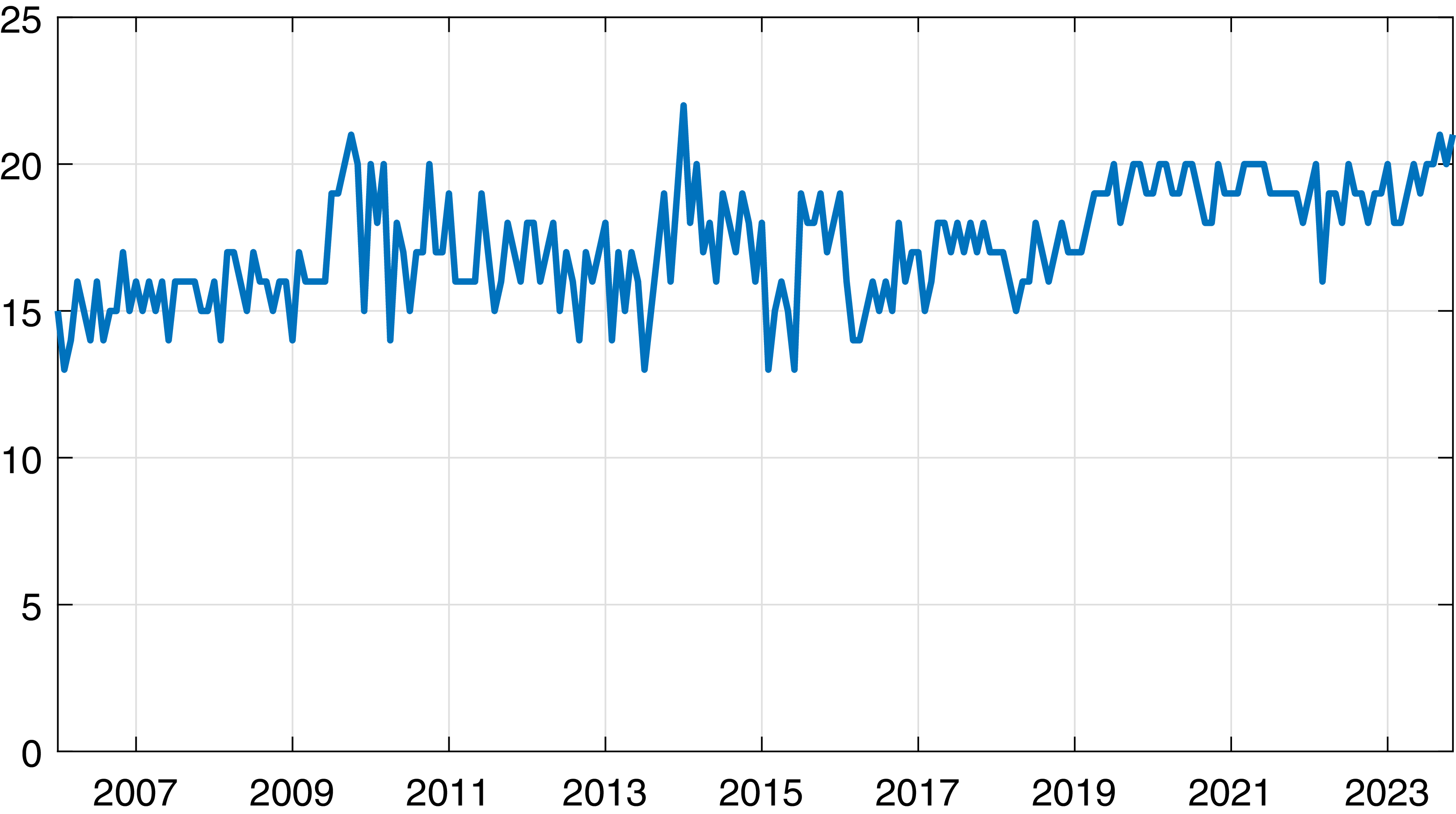
Figure A1 shows the evolution of the number of forecasters submitting inflation forecasts in the Consensus Economics panel for Korea. The number of participants fluctuates between 14 and 21 and is more stable in the last years of the sample period compared to the years before.
Descriptive statistics of individual inflation forecasts

Notes: The table shows the means of the moments of the individual inflation forecasts in each month before and after the change in the BOK’s inflation target.
Number of forecasts in the consensus economics panel.
Notes: The figure shows the number of participants in the monthly Consensus Economics panel for Korea that submitted a forecast for inflation.

Appendix B. Data sources
-
• Consumer Price Index: CPI for all items, not seasonally adjusted, FRED: https://fred.stlouisfed.org/series/KORCPIALLMINMEI, transformation: y–o–y percentage growth rate.
-
• Industrial Production Index: Total Industry excluding construction for Korea, seasonally adjusted, FRED: https://fred.stlouisfed.org/series/KORPROINDMISMEI, transformation: y-o-y percentage growth rate.
-
• Unemployment: Unemployment rate, all persons aged 15–64, seasonally adjusted, FRED: https://fred.stlouisfed.org/series/LRUN64TTKRM156S, transformation: none.
-
• U.S. Yield: Market yield on U.S. Treasury securities at 2-year constant maturity, FRED: https://fred.stlouisfed.org/series/GS2, transformation: none.
-
• Monetary Policy Uncertainty: Series provided by Cho and Kim (Reference Cho and Kim2023) on www.policyuncertainty.com, transformation: none.
-
• VIX index: CBOE volatility index, not seasonally adjusted, monthly average, FRED: https://fred.stlouisfed.org/series/VIXCLS, transformation: log.
-
• Global economic conditions index: Series provided by Baumeister et al. (Reference Baumeister, Korobilis and Lee2022) on https://sites.google.com/site/cjsbaumeister/datasets, transformation: none.
-
• Global price index: Global price index of all commodities, not seasonally adjusted, FRED: https://fred.stlouisfed.org/series/PALLFNFINDEXM, transformation: log.
-
• Expected Inflation (CE): one-year ahead expected inflation from the Consensus Economics panel, accessed through the BOK subscription, transformation: weighted average of calendar-based forecasts.
-
• Expected GDP growth (CE): one-year ahead expected GDP growth from the Consensus Economics panel, accessed through the BOK subscription, transformation: weighted average of calendar based forecasts.
-
• Expected short-term interest rate (CE): one-year ahead expected short-term interest rate from the Consensus Economics panel, accessed through the BOK subscription, transformation: weighted average of calendar based forecasts.
-
• Expected Inflation (BOK): one-year ahead expected inflation from the BOK Consumer Survey, ECOS Economic Statistics System: https://ecos.bok.or.kr, transformation: none.
Appendix C. Robustness checks
C.1. Alternative disagreement measure
In our baseline estimation, the state variable is the cross-sectional standard deviation. We now use two alternative definitions of the state variable, both expressing the disagreement of forecasters about future inflation. The first alternative is the interquartile range of forecasts in a given month, which is less influenced by outliers than the standard deviation. The second is the range between the highest and the lowest inflation forecast in each month. Obviously, this is more susceptible to outliers than the standard deviation.
Figure C1 shows the results for the interquartile range, while Figure C2 shows the estimates based on the spread between the maximum and minimum inflation forecast in each month. All our main findings survive for these alternative state variables. Hence, our results appear robust with respect to the definition of forecast disagreement. As discussed before, these measures are all based on the disagreement among professional forecasters asthe BOK’s survey among consumers does not allow us to calculate a meaningful measure of forecast dispersion.
In addition, the transition function implemented in the main part of the paper transforms the three-month (backward-looking) moving average of the cross-sectional standard deviation into the
 $(0,1)$
interval in order to indicate the prevalence of states. Figure C3 shows the results based on the non-smoothed standard deviation across forecasters. The results remain unchanged.
C.2. Alternative transition function
In Figure C4, we show the estimated impulse responses from the state-dependent model in which the transition between states is driven by an alternative transition function. Instead of the logistic transition function used before, we simply use the empirical cumulative distribution function of the state variable following Born et al. (Reference Born, Müller and Pfeifer2020) to map disagreement into the
 $(0,1)$
interval. The advantage of this specification is that it does not require us to parameterize the transition function (3). All main results remain unchanged.
Effect of monetary policy shock: interquartile range across forecasters.
Notes: The first two panels show the estimated
 $\beta _{h}$
coefficients in the high- and low-disagreement states as a function of
 $h$
as well as 68 and 90% confidence bands constructed from Driscoll and Kraay (Reference Driscoll and Kraay1998) standard errors. The shock is scaled such that the coefficients show the impact of a shock of 10 basis points. Disagreement is measured as the interquartile range across forecasters. The third panel shows the
 $t-$
statistic for the hypothesis of equal
 $\beta _{h}$
coefficients in the high- and low-disagreement states. The gray areas show critical values at the 68% and 90% confidence level.

Effect of monetary policy shock: spread between max and min forecasts.
Notes: The first two panels show the estimated
 $\beta _{h}$
coefficients in the high- and low-disagreement states as a function of
 $h$
as well as 68% and 90% confidence bands constructed from Driscoll and Kraay (Reference Driscoll and Kraay1998) standard errors. The shock is scaled such that the coefficients show the impact of a shock of 10 basis points. Disagreement is measured as the spread between the maximum and the minimum forecast across forecasters. The third panel shows the
 $t$
-statistic for the hypothesis of equal
 $\beta _{h}$
coefficients in the high- and low-disagreement states. The gray areas show critical values at the 68% and 90% confidence level.

Effect of monetary policy shock: non-smoothed disagreement.
Notes: The first two panels show the estimated
 $\beta _{h}$
coefficients in the high- and low-disagreement states as a function of
 $h$
as well as 68% and 90% confidence bands constructed from Driscoll and Kraay (Reference Driscoll and Kraay1998) standard errors. The shock is scaled such that the coefficients show the impact of a shock of 10 basis points. Disagreement is measured as the standard deviation across forecasters. The third panel shows the
 $t-$
statistic for the hypothesis of equal
 $\beta _{h}$
coefficients in the high- and low-disagreement states. The gray areas show critical values at the 68% and 90% confidence level.

Effect of monetary policy shock: alternative transition function.
Notes: The first two panels show the estimated
 $\beta _{h}$
coefficients in the high- and low-disagreement states as a function of
 $h$
as well as 68% and 90% confidence bands constructed from Driscoll and Kraay (Reference Driscoll and Kraay1998) standard errors. The shock is scaled such that the coefficients show the impact of a shock of 10 basis points. Disagreement is measured as the standard deviation across forecasters. The transition between states is driven by the empirical cumulative distribution function of forecast disagreement following Born et al. (Reference Born, Müller and Pfeifer2020). The third panel shows the
 $t-$
statistic for the hypothesis of equal
 $\beta _{h}$
coefficients in the high- and low-disagreement states. The gray areas show critical values at the 68% and 90% confidence level.

C.3. Alternative monetary policy shocks
Figure C5 shows the estimated coefficients from a model with the change of the 12-month KORIBOR as a measure of monetary policy surprises. Unemployment increases under low disagreement but decreases under high disagreement. Similarly, expected GDP growth one-year ahead falls if disagreement is low and rises under high disagreement. For realized and expected inflation, the results are not clear-cut. This could be due to the fact that the change in the 12-month KORIBOR does not seem to reflect the tightening surprises at the end of our sample period, as discussed in the main part of the paper.
Effect of monetary policy shock: change in 12-month KORIBOR.
Notes: The first two panels show the estimated
 $\beta _{h}$
coefficients in the high- and low-disagreement states as a function of
 $h$
as well as 68% and 90% confidence bands constructed from Driscoll and Kraay (Reference Driscoll and Kraay1998) standard errors. The shock is scaled such that the coefficients show the impact of a shock of 10 basis points. Disagreement is measured as the standard deviation across forecasters. The third panel shows the
 $t-$
statistic for the hypothesis of equal
 $\beta _{h}$
coefficients in the high- and low-disagreement states. The gray areas show critical values at the 68% and 90% confidence level.

Also, we observe that numerous BOK meetings held around the end of the month since 2017. Surprises from the end-of-month monetary policy meeting mainly influence variables not this month but next month. Ignoring such a timing issue of meetings potentially generates puzzling contemporaneous responses. Therefore, we follow Gertler and Karadi (Reference Gertler and Karadi2015) and construct a cumulative daily surprise series by cumulating all monetary policy meeting surprises, taking a monthly average of this series, and taking the first difference of this series. We refer to these series as smoothed shocks. Figure C6 shows the corresponding impulse response coefficients. Compared to the main part of this paper, all results remain qualitatively unchanged.
Effect of monetary policy shock: smoothed shock series.
Notes: The first two panels show the estimated
 $\beta _{h}$
coefficients in the high- and low-disagreement states as a function of
 $h$
as well as 68% and 90% confidence bands constructed from Driscoll and Kraay (Reference Driscoll and Kraay1998) standard errors. The shock is scaled such that the coefficients show the impact of a shock of 10 basis points. Disagreement is measured as the standard deviation across forecasters. The third panel shows the
 $t-$
statistic for the hypothesis of equal
 $\beta _{h}$
coefficients in the high- and low-disagreement states. The gray areas show critical values at the 68% and 90% confidence level.

C.4. Distribution of monetary policy shock across states
How different is our baseline monetary policy shock in the two states? Figure C7 provides the histogram of the shock in the high- and low-disagreement states. In order to gauge the realizations on meeting days, the right panel of the figure excludes all observations on non-meeting days of the BOK. Tightening and expansionary monetary policy shocks are largely evenly distributed across periods of high and low inflation disagreement. This indicates that our main finding of weakened monetary policy transmission under the high inflation disagreement is not mainly due to the asymmetric transmission effects of tightening and expansionary monetary policy shocks. We also observe that the variation of shocks is wider in the high disagreement state compared to the low disagreement, which implies that relatively large changes in interest rates and, therefore, inflation tend to be associated with high inflation disagreement.
Distribution of monetary policy shock.
Notes: The figure shows histograms of the monetary policy shock. The blue bars reflect the distribution of
 $F(\widehat {dis}_{t-1}) \times \varepsilon _{t}$
, while the red bars reflect
 $(1-F(\widehat {dis}_{t-1})) \times \varepsilon _{t}$
. The left panel includes all observations, while the right panel excludes months without a BOK policy meeting. The KolmogorovSmirnov test statistic for the null hypothesis that both series are from the same distribution is 0.04 (
 $p=0.99$
) for the left panel and 0.13 (
 $p=0.66)$
for the right panel.