1. Introduction and main results
The question of what can be said about the symplectic image of the Euclidean ball has its roots in Gromov’s celebrated non-squeezing theorem [Reference GromovGro85], one of the most striking and fundamental results in symplectic topology. In this paper we use the periodic Toda lattice to study this question for some Lagrangian products in the classical phase space. More precisely, given
 $A,B \subset {\mathbb{R}}^n$
with non-empty interior, the Lagrangian product of A and B is
 \[ A \times_L B := \{(x_1,y_1,\ldots,x_n,y_n) \in {\mathbb{R}}^{2n} \ | \ (x_1,\ldots,x_n) \in A \ \mathrm{and} \ (y_1,\ldots,y_n) \in B\},\]
endowed with the restriction of the standard symplectic form
 $\omega_0 = \sum_{i=1}^n dx_i \wedge dy_i$
.
Question 1.1. For which
 $A, B \subset {{\mathbb{R}}}^n$
is
 $A \times_L B$
a symplectic ball?Footnote
1
Lagrangian products arise naturally in the study of the dynamics of Minkowski billiards [Reference Artstein-Avidan and OstroverAO14], and play an important role in the connection between Viterbo’s volume-capacity conjecture [Reference ViterboVit00] and Mahler’s conjecture [Reference MahlerMah39] established in [Reference Artstein-Avidan, Karasev and OstroverAKO14]. This motivated the study of symplectic embedding problems for Lagrangian products (see [Reference OstroverOst14, §5]), which started in [Reference RamosRam17], and was subsequently continued in [Reference Ostrover and RamosOR22, Reference Ramos and SepeRS19].
To the best of our knowledge, up to scaling and affine symplectic transformations, there are not too many cases for which the answer to Question 1.1 is known. A well-known example is the Lagrangian product
 $\Diamond^n \times_L \Box^n$
, where
 $\Diamond^n$
is the standard octahedron in
 ${\mathbb{R}}^n$
(i.e., the convex hull of
 $\{\pm e_1, \pm e_2, \ldots, \pm e_n\}$
), and
 $\Box^n = [0,1]^n$
is the standard cube in
 ${{\mathbb{R}}}^n$
. The symplectomorphism between the interiors for
 $n=2$
appeared in [Reference Latschev, McDuff and SchlenkLMS13] (the proof therein uses a deep four-dimensional result of McDuff [Reference McDuffMcD91]), and more recently in [Reference Ramos and SepeRS19] for any dimension (cf. [Reference SchlenkSch05a]). For the Lagrangian product
 $\triangle^n \times_L \Box^n$
, where
 $\triangle^n$
is the standard simplex in
 ${\mathbb{R}}^n$
(i.e., the convex hull of
 $\{0, e_1, e_2, \ldots, e_n\}$
), the following is known:
 $\triangle^n \times_L \Box^n$
embeds symplectically into the Euclidean ball of an arbitrarily close volume, and vice versa (see [Reference Latschev, McDuff and SchlenkLMS13, Reference SchlenkSch05b, Reference TraynorTra95], cf. [Reference RudolfRud22]). Moreover, if
 $n=2$
, the results in [Reference McDuffMcD91] imply that the interior of
 $\triangle^2 \times_L \Box^2$
is symplectomorphic to an open ball. We observe that one can also prove the existence of a symplectomorphismFootnote
2
between the interiors of
 $\triangle^n \times_L \Box^n$
and a Euclidean ball using the strategy of [Reference Ramos and SepeRS19] with a suitable integrable system.
In this paper we provide another answer to Question 1.1. We use the periodic Toda lattice to show that the Lagrangian product of a certain simplex and the Voronoi cell of the root lattice
 $A_n$
(see [Reference Conway and SloaneCS88, Chapter 21, §3.B]) is symplectically equivalent to a Euclidean ball. To state the result precisely, in what follows we identify
 ${{\mathbb{R}}}^{n-1}$
with the hyperplane
 \[W^{n-1}=\{(x_1,\dots,x_{n})\in{{\mathbb{R}}}^{n}\mid x_1+\dots+x_{n}=0\} \subset {{\mathbb{R}}}^{n}.\]
Let
 $S_{n}$
be the symmetric group on n. The above hyperplane is invariant under the
 $S_n$
-action on
 ${{\mathbb{R}}}^{n}$
that permutes the coordinates. We consider the open sets
 \begin{equation}\begin{aligned}\mathfrak{S}^{n-1} & = \left\{ (x_1,\ldots,x_{n}) \in W^{n-1} \ | \ x_{i} - x_{i+1} < 1 \ \mathrm{for} \ 1{\leqslant} i {\leqslant} n, \, x_{n+1} := x_1 \right\} ,\\\mathfrak{P}^{n-1}&= \left\{ (x_1,\ldots,x_{n}) \in W^{n-1} \ | \ \max\{x_1,\ldots x_n\}-\min\{x_1,\ldots x_n\}< 1 \right\}.\end{aligned}\end{equation}
The set
 $\mathfrak{S}^{n-1}$
is the interior of the
 $(n-1)$
-simplex given by the convex hull of the n cyclic permutations of the vector
 \[ \bigg(-{\frac {n-1} 2}, -{\frac {n-1} 2}+1, \ldots, {\frac {n-1} 2}-1,{\frac {n-1} 2} \bigg) \in W^{n-1}.\]
Note that the barycenter of
 $\mathfrak{S}^{n-1}$
is at the origin. The set
 $\mathfrak{P}^{n-1}$
is the convex hull of the n cyclic permutations of the vectors
 \[\bigg(\frac{1}{n},\dots,\frac{1}{n},-\frac{n-1}{n}\bigg)\quad\text{and}\quad\bigg(-\frac{1}{n},\dots,-\frac{1}{n},\frac{n-1}{n}\bigg).\]
The polytope
 $\mathfrak{P}^{n-1}$
can be described in terms of a difference body as we explain next. Consider the simplex
 \[\triangle^{n-1} = \mathrm{Conv} \{ e_1, \ldots , e_{n} \} \subset {{\mathbb{R}}}^n,\]
where Conv denotes the convex hull. Let
 $\tau_{-b} \colon {{\mathbb{R}}}^n \to {{\mathbb{R}}}^n$
be the translation by the negative of the vector
 $b = \frac{1}{n}\sum_{i=1}^n e_n$
. Since b is the barycenter of
 $\triangle^{n-1}$
, the barycenter of the simplex
 $\triangle_W^{n-1} := \tau_{-b}(\triangle^{n-1})$
is at the origin; moreover, by construction,
 $\triangle_W^{n-1} \subset W$
. By definition of
 $\triangle_W^{n-1}$
, the support function of the difference body
 $ \triangle_W^{n-1}-\triangle_W^{n-1}$
is given by
 \begin{align*} h_{\triangle_W^{n-1}-\triangle_W^{n-1}}(x) & = \max \{x_i - \langle x, b\rangle \mid i = 1,\ldots, n \} - \min\{x_i - \langle x, b\rangle \mid i = 1,\ldots, n \} \\& = \max\{x_1,\ldots x_n\}-\min\{x_1,\ldots x_n\},\end{align*}
where we recall that the support function of a convex body
 $ K \subset {\mathbb{R}}^{n-1}$
is given by
 $h_K(x) = \sup \{ \langle x,y \rangle <1 \mid y\in K \}$
. Hence, by (1), the polytope
 $\mathfrak{P}^{n-1}$
is the polar body of
 $ \triangle_W^{n-1}-\triangle_W^{n-1}$
. (In fact, it is also the polar body of
 $\triangle^{n-1} - \triangle^{n-1}$
.) Such polytopes are sometimes known as ‘generalized rhombic dodecahedra’ (see, for example, [Reference ŽivaljevićZiv15]). In particular, for
 $n=3$
, the set
 $\mathfrak{P}^2$
is a regular hexagon, and for
 $n=4$
, the set
 $\mathfrak{P}^3$
is a rhombic dodecahedron (see Figure 1). Since the two simplices
 $\mathfrak{S}^{n-1}$
and
 $\triangle_W^{n-1}$
share the same barycenter, one can construct a map
 $A \in \mathrm{SL}(n)$
such that
 $\mathfrak{P}^{n-1} $
is the dual of the difference body of
 $A \mathfrak{S}^{n-1}$
.
A rhombic dodecahedron (the dual of the difference body of a simplex)Footnote 3 .

The subspace
 $V^{2n-2}=W^{n-1}\times_L W^{n-1}\subset{{\mathbb{R}}}^{2n}$
is symplectic. Hence, in what follows we may identify
 $V^{2n-2}$
with
 ${{\mathbb{R}}}^{2n-2}$
symplectically, so that we may consider Lagrangian products of the form
 $A \times_L B$
, where
 $A, B \subset W^{n-1}$
. Moreover, we use the following notation for a Euclidean ball in
 ${{\mathbb{R}}}^{2n-2}$
:
 \[B^{2n-2}(a) := \{(x_1,y_1,\dots,x_{n-1},y_{n-1})\in{{\mathbb{R}}}^{2n-2}\mid \pi\big(x_1^2+y_1^2+\dots+x_{n-1}^2+y_{n-1}^2\big)<a\}.\]
The precise (partial) answer to Question 1 is the following result.
Theorem 1.2. The Lagrangian product
 $\mathfrak{S}^{n-1} \times_L \mathfrak{P}^{n-1}$
is symplectically equivalent to
 $B^{2n-2}(n)$
, that is, for every
 $\epsilon>0$
, there exist symplectic embeddings
 \[(1-\epsilon)\big(\mathfrak{S}^{n-1} \times_L \mathfrak{P}^{n-1} \big)\hookrightarrow B^{2n-2}(n)\hookrightarrow(1+\epsilon)\big(\mathfrak{S}^{n-1} \times_L \mathfrak{P}^{n-1}\big).\]
We observe that, for
 $n=3$
, Theorem 1.2 also implies a partial answer to [Reference BalitskiyBal20, Question 4.4] (cf. [Reference RudolfRud22, Theorems 1.2 and 1.3]). Indeed, in this case, it follows from this theorem that the Lagrangian product of an equilateral triangle T and the hexagon
 $T-T$
rotated by
 $\pi/6$
is symplectomorphic to a Euclidean ball in
 ${\mathbb{R}}^4$
. More precisely, the following corollary holds.
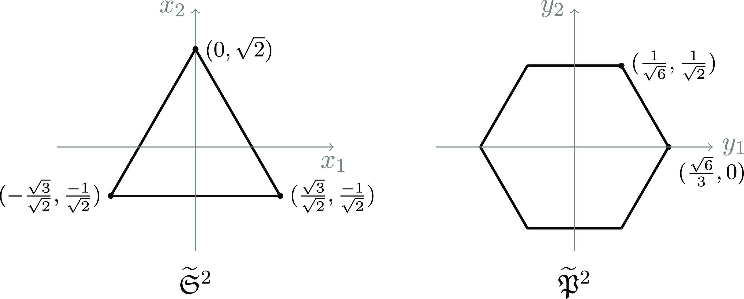
Corollary 1.3. The interior of the Lagrangian product of the equilateral triangle and the regular hexagon of Figure 2 is symplectomorphic to the interior of a symplectic ball.
The product
 $\widetilde{\mathfrak{S}}^2 \times_L \widetilde{ \mathfrak{P}}^2$
is symplectomorphic to a Euclidean ball.

Proof. If
 $n=2$
, then
 $\mathfrak{S}^2$
is the interior of the equilateral triangle
 \[ \mathrm{Conv} \bigl \{ (-1,0,1),(1,-1,0),(0,1,-1) \bigr \} \subset W^2,\]
and
 $\mathfrak{P}^2 $
is the interior of the regular hexagon
 \begin{align*} \mathfrak{P}^2 = \mathrm{Conv} & \left\{ \left({\frac {-2} 3},{\frac 1 3},{\frac 1 3}\right),\left({\frac 1 3},{\frac {-2} 3},{\frac 1 3}\right),\left({\frac 1 3},{\frac 1 3},{\frac {-2} 3}\right) , \left({\frac {2} 3},{\frac {-1} 3},{\frac {-1} 3}\right),\left({\frac {-1} 3},{\frac {2} 3},{\frac {-1} 3}\right),\right.\\& \quad \left. \left({\frac {-1} 3},{\frac {-1} 3},{\frac {2} 3}\right)\right\} \subset W^2.\end{align*}
Note that the Lagrangian product
 $\mathfrak{S}^2 \times_L \mathfrak{P}^2$
is symplectomorphic to
 $\widetilde {\mathfrak{S}}^2 \times_L \widetilde{ \mathfrak{P}}^2$
, where
 $\widetilde {\mathfrak{S}}^2 = A \mathfrak{S}^2$
,
 $\widetilde {\mathfrak{P}}^2 = (A^T)^{-1} \mathfrak{P}^2$
, and
 $A \in \mathrm{O}(3)$
is the orthogonal transformation that rotates the plane
 $x_1+x_2+x_3=0 $
in
 ${\mathbb{R}}^3$
to the plane
 $x_3=0$
so that
 $\widetilde{\mathfrak{S}}^2$
and
 $\widetilde{\mathfrak{P}}^2$
are as in Figure 2. Hence, by Theorem 1.2, the Lagrangian product
 $\widetilde{\mathfrak{S}}^2 \times_L \widetilde {\mathfrak{P}}^2$
is symplectically equivalent to a Euclidean ball. By [Reference Latschev, McDuff and SchlenkLMS13, Lemma 4.3], the result follows.
Theorem 1.2 follows from the main result of this paper, Theorem 1.4. Intuitively speaking, the latter states that the Lagrangian product of
 $\mathfrak{S}^n$
and a suitable
 $S_{n}$
-invariant region in
 $W^{n-1}$
is symplectically equivalent to a toric domain, that is, a subset of
 ${{\mathbb{R}}}^{2n-2}$
of the form
 \[X_\Omega=\big\{(x_1,y_1,\dots,x_{n-1},y_{n-1})\in{{\mathbb{R}}}^{2n-2}\mid \big(\pi(x_1^2+y_1^2),\dots,\pi(x_{n-1}^2+y_{n-1}^2)\big)\in\Omega\big\},\]
where
 $\Omega\subset {{\mathbb{R}}}^{n-1}_{{\geqslant} 0}$
is a relatively open set. The terminology comes from the fact that, given
 $\Omega \subset {{\mathbb{R}}}^{n-1}_{{\geqslant} 0}$
, the subset
 $X_{\Omega} \subset {{\mathbb{R}}}^{2n-2}$
is invariant under the standard
 $(S^1)^{n-1}$
-action on
 ${{\mathbb{R}}}^{2n-2} \simeq {\mathbb{C}}^{n-1}$
, where
 $S^1 = {{\mathbb{R}}}/{\mathbb{Z}}$
. A Euclidean ball in
 ${{\mathbb{R}}}^{2n-2}$
is an example of a toric domain: given
 $a > 0$
,
 $B^{2n-2}(a) = X_{T(a)}$
, where
 $T(a)=\{(r_1,\dots,r_{n-1})\in{{\mathbb{R}}}^{n-1}_{{\geqslant} 0}\mid r_1+\dots+r_{n-1}<a\}$
.
In order to state Theorem 1.4, we need to introduce some more notions. In what follows we restrict our discussion to subsets of
 $W^{n-1}$
that are
 $S_{n}$
-invariant. To any such subset we may naturally associate a subset of
 ${{\mathbb{R}}}^{n-1}_{{\geqslant} 0}$
as follows: for any
 $(y_1,\ldots, y_{n}) \in {{\mathbb{R}}}^{n}$
, there exists
 $\sigma \in S_{n}$
such that
 $y_{\sigma(1)}{\leqslant} \cdots {\leqslant} y_{\sigma(n)}$
. Although such a permutation may not be unique, the vector
 \begin{equation} \rho(y_1,\dots,y_{n}):=n \big(y_{\sigma(2)}-y_{\sigma(1)},y_{\sigma(3)}-y_{\sigma(2)},\dots,y_{\sigma(n)}-y_{\sigma(n-1)} \big) \end{equation}
does not depend on the choice of permutation. Hence, the map
 $\rho \colon {{\mathbb{R}}}^{n} \to {{\mathbb{R}}}^{n-1}_{{\geqslant} 0}$
is well defined. To an
 $S_{n}$
-invariant subset
 $A \subset W^{n-1}$
we associate
 $\rho(A) \subset {{\mathbb{R}}}^{n-1}_{{\geqslant} 0}$
. We remark that if A is
 $S_{n}$
-invariant, the set
 $\rho(A)$
determines A uniquely. Finally, we also say that a set
 $A\subset W^{n-1}$
is star-shaped if
 $rA\subset A$
for all
 $0{\leqslant} r {\leqslant} 1$
. The main result of our paper is the following theorem.
Theorem 1.4. Let
 $A\subset W^{n-1}$
be a subset that is
 $S_{n}$
-invariant, open, bounded and star-shaped. Then the Lagrangian product
 $\mathfrak S^{n-1} \times_L A$
is symplectically equivalent to the toric domain
 $X_{\rho(A)}$
.
Remark 1.5. Given an open, bounded, and star-shaped subset
 $B \subset {{\mathbb{R}}}^{n-1}_{{\geqslant} 0}$
, there exists an
 $S_{n}$
-invariant, open, bounded, and star-shaped
 $A \subset W^{n-1}$
such that
 $\rho(A) = B$
. To see this, observe that the restriction of the map
 $\rho \colon {{\mathbb{R}}}^n \to {{\mathbb{R}}}_{{\geqslant} 0}^{n-1}$
to the subset
 \[W^{n-1}_+:= \{(x_1,\ldots, x_n \in W^{n-1} \mid x_1 {\leqslant} x_2 {\leqslant} \cdots {\leqslant} x_n \}\]
is invertible. Hence, we may define
 $A_+ \subset W^{n-1}_+$
to be the unique pre-image of B under
 $\rho$
. Then A is obtained from
 $A_+$
by reflecting it in each hyperplane given by
 $\{(x_1,\ldots, x_n) \in {{\mathbb{R}}}^n \mid x_i = x_j\}$
for
 $i \neq j$
.
Theorem 1.2 is a simple consequence of Theorem 1.4.
Proof of Theorem 1.2. The subset
 $\mathfrak{P}^{n-1} \subset W^{n-1}$
of (1) is
 $S_{n}$
-symmetric, relatively open, bounded, and convex. For
 $(y_1,\dots,y_{n})\in \mathfrak{P}^{n-1}$
, set
 $(r_1,\dots,r_{n-1}) :=\rho(y_1,\dots,y_{n})$
. By the definition of
 $\rho$
,
 \[r_1+\dots+r_{n-1}=n\big(\max\{y_1,\dots,y_{n}\}-\min\{y_1,\dots,y_{n}\}\big)<n.\]
Conversely, let
 $(r_1,\dots,r_{n-1})\in {{\mathbb{R}}}^{n-1}_{{\geqslant} 0}$
be such that
 $\sum_{i=1}^{n-1} r_i < n$
. For
 $i=1,\dots,n$
, we set
 \[y_i:=\frac{1}{n^2}\sum_{j=1}^{n-1} j r_j-\frac{1}{n}\sum_{j=i}^{n-1} r_j.\]
By a simple calculation, we have that
 $y_1+\dots+y_{n} = 0$
, and
 \[\max\{y_1,\dots,y_{n}\}-\min\{y_1,\dots,y_{n}\}=y_{n}-y_1=\frac{1}{n}\sum_{j=1}^{n-1} r_j<1.\]
Hence,
 $ \rho(\mathfrak{P}^{n-1})=T(n)$
and then
 $X_{\rho(\mathfrak{P}^{n-1})}=B^{2n-2}(n)$
. By Theorem 1.4, the Lagrangian product
 $\mathfrak{S}^{n-1}\times_L \mathfrak{P}^{n-1}$
is symplectically equivalent to
 $B^{2n-2}(n)$
.
While the strategy of the proof of Theorem 1.4 is somewhat similar to that of the main result in [Reference Ramos and SepeRS19], the ingredients are substantially more involved. The one-parameter family of integrable systems that we use to construct the desired symplectic embeddings comes from the periodic Toda lattice (see [Reference Adler, van Moerbeke and VanhaeckeAMV04, Reference FlaschkaFla74a, Reference FlaschkaFla74b, Reference HénonHen74, Reference TodaTod65a] and references therein). It is known that this system admits global action-angle variables (see [Reference Flaschka and McLaughlinFM76, Reference Henrici and KappelerHK08b, Reference van MoerbekevMo76]). The proof of Theorem 1.4 hinges on showing certain properties of the global action variables as a certain parameter goes to infinity (see Proposition 4.4), and the combination of these properties with the results in [Reference Flaschka and McLaughlinFM76, Reference Henrici and KappelerHK08b, Reference van MoerbekevMo76]. In particular, we show that the standard billiard in (the closure of)
 $\mathfrak{S}^{n-1}$
can be thought of as a limit of a suitable one-parameter deformation of the standard Toda lattice (see Lemma 4.2 and Remark 4.3). We believe that this result should be of independent interest.
Since the proof of Theorem 1.4 involves the periodic Toda Hamiltonian associated with the root system
 $A_n$
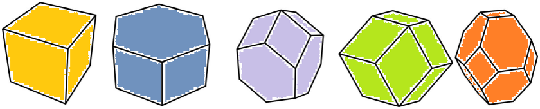
, we speculate that the study of the more general periodic Toda potentials considered in [Reference BogoyavlenskyBog76] and [Reference Adler, van Moerbeke and VanhaeckeAMV04, Chapter 9] might lead to different solutions to Question 1.1. In fact, going even further, we expect that more interesting results in symplectic topology can be obtained by studying the relation between classical integrable systems and billiards. In particular, one possible candidate is the Lagrangian product of a simplex and a permutohedron in a certain position. Indeed, it was proved in [Reference BalitskiyBal20] that the Lagrangian product of a simplex and a permutohedron (properly related to each other) delivers equality in Viterbo’s conjecture [Reference ViterboVit00]. It is plausible that one can use the same strategy of proof as in Theorem 1.4 to show that the above Lagrangian product is symplectically equivalent to a Euclidean ball, thus obtaining a complete answer to [Reference BalitskiyBal20, Question 4.4]. Moreover, in dimension 3, motivated by Theorem 1.2, we can generalize from [Reference BalitskiyBal20, Question 4.4] as follows. Recall that in dimension 3 there are five space-filling polytopes that tile the space by translations (also known as parallelohedra or Fedorov solids; see [Reference Conway and SloaneCS92] and Figure 3).
The five Fedorov solids (from left to right): the cube, the hexagonal prism, the elongated dodecahedron, the rhombic dodecahedron, and the truncated octahedron.

Conjecture 1.6. The Lagrangian product of a three-dimensional simplex and any one of the five parallelohedra in an appropriate linear position is symplectically equivalent to a Euclidean ball.
In addition to the two known cases of the cube and the rhombic dodecahedron, Conjecture 1.6 is supported by the fact that all the aforementioned Lagrangian products deliver equality in Viterbo’s conjecture [Reference ViterboVit00]. Indeed, the case of the permutohedron follows from the main result of [Reference BalitskiyBal20], and in the remaining two cases the systolic ratio in Viterbo’s conjecture can be explicitly computed based on the main result of [Reference Haim-KislevHai19].
1.1 Structure of the paper
In § 2 we show how to use Theorem 1.4 to construct Lagrangian products that are symplectomorphic to ellipsoids and polydisks in dimension 4 (similar examples could be obtained also in higher dimensions). In § 3 we recall some known facts regarding the periodic Toda lattice, and construct a certain symplectomorphism that plays an important role in the proof of our main result. Section 4 is the technical heart of the paper and contains the proof of Theorem 1.4.
2. Some examples in dimension 4
In this section we use Theorem 1.4 to construct Lagrangian products that are either symplectically equivalent or symplectomorphic to ellipsoids or polydisks in dimension 4.
2.1 Ellipsoids and polydisks
For
 $a,b>0$
consider the open ellipsoid and the polydisk in
 ${\mathbb{C}}^2$
given by
 \[ E(a,b) = \bigg\{ (z_1,z_2) \, | \, {\frac {\pi|z_1|^2} {a} } + {\frac {\pi|z_2|^2} {b}} < 1 \bigg\}, \quad P(a,b) = \bigg\{ (z_1,z_2) \, | \, {\frac {\pi|z_1|^2} {a} } < 1, \, {\frac {\pi|z_2|^2} {b}} < 1 \bigg\}.\]
Both E(a,b) and P(a,b) are toric domains: the moment map image of the former is the triangle with vertices (0, 0), (a, 0), and (0, b) with the edge joining (a,0) and (0,b) removed, while that of the latter is the rectangle with vertices (0, 0), (a, 0), (0, b),(a, b) with the sides joining (a,0) and (a,b), and (0,b) and (a,b), removed. In analogy with Theorem 1.2, in what follows we describe Lagrangian product configurations that are symplectically equivalent to either E(a,b) or P(a,b).
First, we deal with the case of the ellipsoid E(a,b). Consider the set
 \[\mathfrak{P}_E^2[a,b] := \bigsqcup_{\sigma \in S_3} \sigma \cdot T[a,b] \subset W^2\]
that is the union of the six open triangles obtained by the action of
 $S_3$
on the interior of the triangle
 \[ T[a,b] := \mathrm{Conv} \bigg\{ (0,0,0), \bigg({\frac {-2a} 3},{\frac a 3},{\frac a 3}\bigg),\bigg({\frac {-b} 3},{\frac {-b}{3}},{\frac {2b} 3}\bigg) \bigg\}.\]
Set
 $\widetilde{\mathfrak{S}}^2 = A \mathfrak{S}^2$
, and
 $\widetilde{\mathfrak{P}}_E^2[a,b] = (A^{T})^{-1} \mathfrak{P}^2_E[a,b]$
, where
 $A \in \mathrm{O}(3)$
rotates the plane
 $x_1+x_2+ x_3=0 $
to the plane
 $x_3=0$
. Assume for simplicity that
 $0<a<b$
. The closure of
 $\widetilde{\mathfrak{P}}_E^2[a,b]$
(in the
 $\{x_1,x_2\}$
-plane) is the hexagon with a counterclockwise sequence of vertices given by
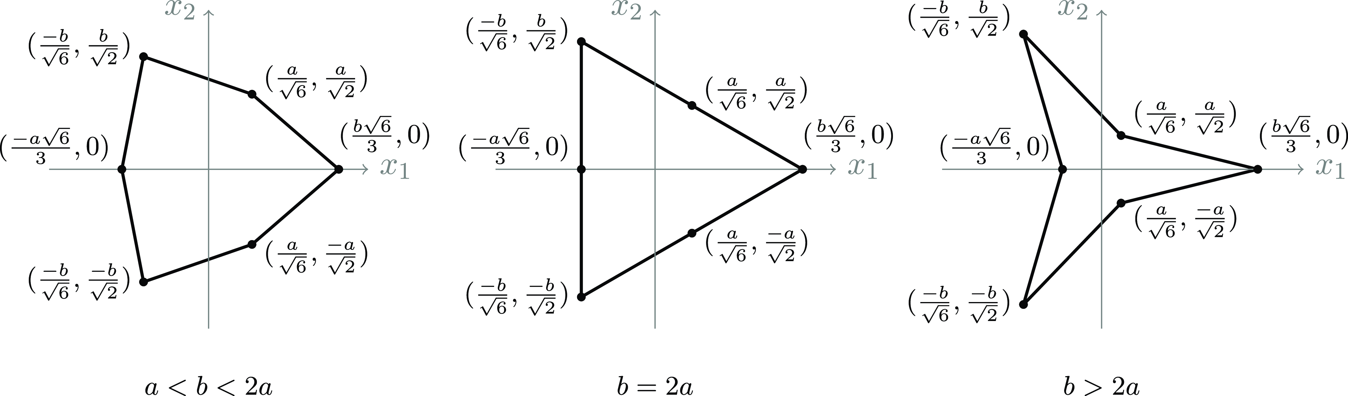
 \[\bigg\{\bigg({\frac {b\sqrt{6}} {3} },0 \bigg), \bigg({\frac {a} {\sqrt{6}}},{\frac {a} {\sqrt{2}} } \bigg) , \bigg ({\frac {-b} {\sqrt{6}}},{\frac {b} {\sqrt{2}} } \bigg) , \bigg({\frac {-a\sqrt{6}} {3} },0 \bigg),\bigg ({\frac {-b} {\sqrt{6}}},{\frac {-b} {\sqrt{2}} } \bigg),\bigg({\frac {a} {\sqrt{6}}},{\frac {-a} {\sqrt{2}} } \bigg) \bigg\}.\]
The above hexagon is convex when
 $b<2a$
, concave when
 $b>2a$
, and degenerates to an equilateral triangle when
 $b=2a$
(see Figure 4).
The (possibly degenerate) hexagons that are the closure of
 $ \mathfrak{P}_E^2[a,b]$
for various values of
 $a,b >0$
.

By construction,
 $ \mathfrak{P}_E^2[a,b]$
is
 $S_3$
-invariant, open, bounded, and star-shaped; moreover, its image under the map
 $\rho:{{\mathbb{R}}}^{3}\to{{\mathbb{R}}}^{n}_{{\geqslant} 0}$
defined in (2) is the open triangle with vertices (0, 0), (a, 0), and (0, b). Hence, the following result is an immediate consequence of Theorem 1.4.
Corollary 2.1. The Lagrangian product
 $\mathfrak{S}^2 \times_L \mathfrak{P}_E^2[a,b]$
is symplectically equivalent to E(3a,3b).
We can strengthen Corollary 2.1 to the following result.
Corollary 2.2 For all
 $a,b>0$
,
 $\mathfrak S^2 \times_L \mathfrak{P}_E^2[a,b]$
is symplectomorphic to E(3a,3b).
Proof. The argument is identical to that of [Reference Latschev, McDuff and SchlenkLMS13, Corollary 4.2 and Lemma 4.3] with the only difference that we use [Reference McDuffMcD09, Corollary 1.6(i)] instead of [Reference McDuffMcD91].
The case of the polydisk P(a,b) is very similar. Define the set
 \[ \mathfrak{P}_P^2[a,b] := \bigsqcup_{\sigma \in S_3} \sigma \cdot Q[a,b] \subset W^2,\]
where Q[a,b] is the interior of the parallelogram given by
 \[Q[a,b] := \mathrm{Conv} \bigg\{ (0,0,0), \bigg({\frac {-2a} 3},{\frac a 3},{\frac a 3}\bigg),\bigg({\frac {-b} 3},{\frac {-b} 3},{\frac {2b} 3}\bigg), \bigg( {\frac {-2a-b} {3} },{\frac {a-b} {3} }, {\frac {a+2b} {3} } \bigg) \bigg\}.\]
Denote
 $\widetilde{\mathfrak{P}}_P^2[a,b] = (A^{T})^{-1} \mathfrak{P}^2_P[a,b]$
, where
 $A \in \mathrm{O}(3)$
as above. The closure of
 $\widetilde{\mathfrak{P}}_P^2[a,b]$
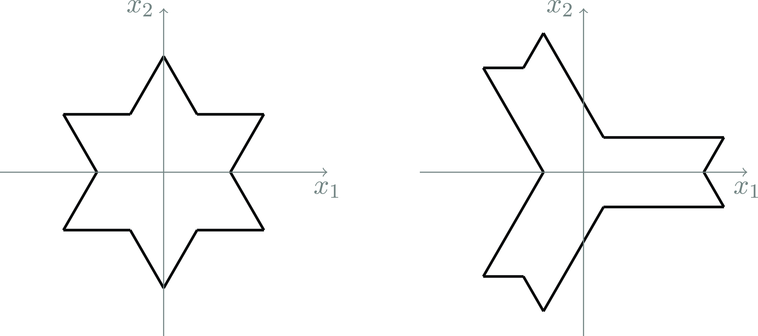
is the dodecagon composed of the six parallelograms obtained from Q[a,b] by the action of
 $S_3$
(see Figure 5) with a counterclockwise sequence of vertices given by
 \begin{align*}&\bigg\{ \bigg({\frac {b\sqrt{6}} {3} },0 \bigg), \bigg( {\frac {b\sqrt{6}} {3} } + {\frac {a} {\sqrt{6}} },{\frac {a} {\sqrt{2}}} \bigg) , \bigg({\frac {a} {\sqrt{6}}},{\frac {a} {\sqrt{2}} } \bigg) , \bigg( {\frac {a-b} {\sqrt{6}}} , {\frac {a+b} {\sqrt{2}}}\bigg) , \bigg({\frac {-b} {\sqrt{6}}},{\frac {b} {\sqrt{2}} } \bigg) , \bigg({\frac {-b} {\sqrt{6}}} - {\frac {a\sqrt{6}} {3} } , {\frac {b} {\sqrt{2}}} \bigg), \\&\quad \bigg({\frac {-a\sqrt{6}} {3} },0 \bigg),\bigg({\frac {-b} {\sqrt{6}}} - {\frac {a\sqrt{6}} {3} } , {\frac {-b} {\sqrt{2}}} \bigg), \bigg({\frac {-b} {\sqrt{6}}},{\frac {-b} {\sqrt{2}} } \bigg), \bigg( {\frac {a-b} {\sqrt{6}} }, {\frac {-a-b} {\sqrt{2}} } \bigg), \bigg({\frac {a} {\sqrt{6}}},{\frac {-a} {\sqrt{2}} } \bigg),\\&\quad \bigg( {\frac {b\sqrt{6}} {3} } + {\frac {a} {\sqrt{6}} } ,{\frac {-a} {\sqrt{2}} }\bigg) \bigg\}.\end{align*}
The dodecagons that are the closure of
 $\widetilde{\mathfrak{P}}_P^2[1,1]$
(left) and
 $\widetilde{\mathfrak{P}}_P^2[1,3]$
(right).

The set
 $ \mathfrak{P}_P^2[a,b]$
is
 $S_3$
-invariant, open, bounded, star-shaped and its image under
 $\rho$
is the open rectangle with vertices (0, 0), (a, 0), (b,0), and (a, b). Hence, the following result is an immediate consequence of Theorem 1.4.
Corollary 2.3. The Lagrangian product
 $\mathfrak{S}^2 \times_L \mathfrak{P}_P^2[a,b]$
is symplectically equivalent to the polydisk P(3a,3b) for every
 $a,b>0$
.
3. The periodic Toda lattice
3.1 Integrability via the Lax pair formalism
The periodic Toda lattice [Reference TodaTod65a, Reference TodaTod65b] is a well-known Hamiltonian system on
 ${{\mathbb{R}}}^{2n}$
describing the movement of n labeled particles on a circle with exponential interactions between nearest neighbors. This is one of the earliest examples of a completely integrable non-linear Hamiltonian system [Reference FlaschkaFla74a, Reference HénonHen74, Reference ManakovMan74], and has been studied extensively. Before describing it explicitly, we set all indices to be periodic modulo n unless otherwise stated. (We observe that this is a different convention to that of §§ 1 and 2.) The Hamiltonian function determining the equations of motion of the periodic Toda lattice is
 \[H(q_1,\dots,q_n,p_1,\dots,p_n)=\frac{1}{2}\sum_{i=1}^n p_i^2+\alpha^2 \sum_{i=1}^n e^{q_i-q_{i+1}},\]
where
 $\alpha>0$
is a fixed parameter that can be considered as the strength of the potential. Its equations of motion are given by:
 \[\begin{cases}\dot{q}_i=p_i,\\\dot{p}_i=\alpha^2\big(e^{q_{i-1}-q_i}-e^{q_i-q_{i+1}}\big),\end{cases}\]
where we set
 $q_{n+1}=q_1$
and
 $q_0 = q_n$
. It is well known that the periodic Toda lattice is completely integrable (see, for instance, [Reference FlaschkaFla74a, Reference FlaschkaFla74b, Reference Flaschka and McLaughlinFM76, Reference van MoerbekevMo76] among others). One way to construct the desired integrals of motion is to start with a ‘change of variables’ due to Flaschka [Reference FlaschkaFla74a, Reference FlaschkaFla74b] that describes the motion relative to the center of mass. It is given by the map
 \begin{equation}\begin{aligned}\widetilde{\varphi}_{\alpha} : {{\mathbb{R}}}^{2n} &\to {{\mathbb{R}}}^n \times {{\mathbb{R}}}^n_{>0}, \\(q_1,\ldots, q_n,p_1,\ldots, p_n) &\mapsto (p_1,\dots,p_n,\alpha e^{\frac{q_1-q_2}{2}},\dots,\alpha e^{\frac{q_n-q_1}{2}}).\end{aligned}\end{equation}
We remark that
 $\widetilde{\varphi}_{\alpha}$
is not a diffeomorphism: for instance, the image of
 $\widetilde{\varphi}_{\alpha}$
is contained in the subset
 \[\bigg\{(b_1,\ldots,b_n,a_1,\ldots, a_n) \in {{\mathbb{R}}}^n \times {{\mathbb{R}}}^n_{>0} \,\bigg|\, \prod_{i=1}^n a_i = \alpha^n \bigg\}.\]
If we set
 $\pi_0 := \omega^{-1}_0$
, that is,
 $\pi_0 = \sum_{i=1}^n \frac{\partial }{\partial p_i} \wedge \frac{\partial }{\partial q_i}$
, then
 $\pi_0$
can be pushed forward to a bivector field
 $\pi$
on
 ${{\mathbb{R}}}^n \times {{\mathbb{R}}}^n_{>0}$
. Explicitly,
 \[\pi=\sum_{i=1}^n \frac{a_i}{2}\frac{\partial}{\partial b_i}\wedge \frac{\partial}{\partial a_i}-\sum_{i=1}^n\frac{a_{i-1}}{2}\frac{\partial}{\partial b_i}\wedge \frac{\partial}{\partial a_{i-1}}.\]
Since
 $\pi_0$
is Poisson, by construction
 $\pi$
is also Poisson and the map
 $\widetilde{\varphi}_{\alpha}$
is a Poisson morphism. For our purposes, it is useful to prove the following well-known properties of the Poisson manifold
 $({{\mathbb{R}}}^n \times {{\mathbb{R}}}^n_{>0},\pi)$
.
Lemma 3.1. The Poisson structure
 $\pi$
on
 ${{\mathbb{R}}}^n \times {{\mathbb{R}}}^n_{>0}$
has constant rank equal to
 $2n-2$
and the symplectic leaves are given by the level sets of the map
 \begin{equation}\begin{aligned}{{\mathbb{R}}}^n \times {{\mathbb{R}}}^n_{>0} &\to {{\mathbb{R}}}^2, \\(b_1,\ldots, b_n, a_1,\ldots, a_n) &\mapsto \bigg(\sum_{i=1}^n b_i , \, \prod_{i=1}^n a_i\bigg).\end{aligned}\end{equation}
Proof. Let
 $\{\cdot,\cdot\}$
denote the Poisson bracket on
 $C^{\infty} ({{\mathbb{R}}}^n \times {{\mathbb{R}}}^n_{>0})$
induced by
 $\pi$
. For any
 $i,j = 1,\ldots, n$
, we have that
 $\{b_i,b_j\} = \{a_i,a_j\} = 0$
; moreover,
 $\{b_i,a_j\} = 0$
unless
 $j=i-1$
or
 $j=i$
. Since the matrix
 $(\{b_i,a_j\})$
has rank
 $n-1$
, it follows that
 $\pi$
has constant rank equal to
 $2n-2$
. By a direct computation, the components of map (4) are Casimirs of
 $\pi$
, that is, they have vanishing Hamiltonian vector field. Since the above map is a submersion with connected level sets, and since the rank of
 $\pi$
is equal to
 $2n-2$
, the result follows.
By Lemma 3.1, the submanifold
 \[\mathcal{M}_{\alpha} :=\bigg\{(b_1,\dots,b_n,a_1,\dots,a_n)\in{{\mathbb{R}}}^n\times{{\mathbb{R}}}^n_{> 0}\,\bigg|\,\sum_{i=1}^n b_i=0\text{ and }\prod_{i=1}^n a_i=\alpha^n\bigg\} \subset {{\mathbb{R}}}^n \times {{\mathbb{R}}}^n_{>0}\]
is a leaf in the symplectic foliation of
 $({{\mathbb{R}}}^n \times {{\mathbb{R}}}^n_{>0},\pi)$
for each
 $\alpha >0$
. We denote the symplectic form on
 $\mathcal{M}_{\alpha}$
by
 $\omega_{\alpha}$
. By a direct calculation,
 $\omega_{\alpha}$
is the restriction to
 $\mathcal{M}_{\alpha}$
of the 2-form
 \[2\sum_{i=2}^n \sum_{j=1}^{i-1} db_i\wedge \frac{da_j}{a_j} \in \Omega^2({{\mathbb{R}}}^n \times {{\mathbb{R}}}^n_{>0}).\]
Next, there exists a function
 $\overline{H} \in C^{\infty} ({{\mathbb{R}}}^n \times {{\mathbb{R}}}^n_{>0})$
such that
 $\widetilde{\varphi}^*_{\alpha} \overline{H} = H$
, namely,
 \[ \overline{H}(b_1,\dots,b_n,a_1,\dots,a_n)=\frac{1}{2}\sum_{i=1}^n b_i^2+\sum_{i=1}^n a_i^2.\]
The corresponding equations of motion with respect to
 $\pi$
are
 \begin{equation}\begin{cases}\dot{b}_i=a_{i-1}^2-a_{i}^2,\\\dot{a}_i=\dfrac{a_i}{2}(b_{i}-b_{i+1}).\end{cases}\end{equation}
The key observation from [Reference FlaschkaFla74a] is that (5) admits a description in terms of a Lax pair, that is, a pair of
 $n \times n$
matrices (L,B) such that (5) is equivalent to
 \begin{equation}\dot{L}=[L,B].\end{equation}
Explicitly,
 \begin{equation}L=\begin{bmatrix} b_1&a_1&0&\dots&0&a_n\\ a_1&b_2&a_2&\dots&0&0\\0&a_2&b_3&\ddots&0&0\\\vdots&\vdots&\ddots&\ddots&\ddots&\vdots\\0&0&0&\ddots&\ddots&a_{n-1}\\ a_n&0&0&\dots&a_{n-1}&b_n\end{bmatrix},\quad B=\frac{1}{2}\begin{bmatrix}0&a_1&0&\dots&0&-a_n\\-a_1&0&a_2&\dots&0&0\\0&-a_2&0&\ddots&0&0\\\vdots&\vdots&\ddots&\ddots&\ddots&\vdots\\0&0&0&\ddots&\ddots&a_{n-1}\\ a_n&0&0&\dots&-a_{n-1}&0\end{bmatrix}.\end{equation}
We denote the eigenvalues of L by
 $\lambda_1^+{\leqslant} \cdots{\leqslant} \lambda_n^+$
(the reason for the ‘
 $+$
’ becomes apparent below, after (22)). By (6), these are conserved, and so is
 $\mathrm{Tr}(L) = \sum_{i=1}^n b_i$
. If we set
 $W^{n-1}_{+}=\{(y_1,\dots,y_n)\in W^{n-1}\mid y_1{\leqslant} \cdots {\leqslant} y_n\}$
, the map
 $F_\alpha:\mathcal{M}_\alpha\to W^{n-1}_{+}$
,
 \begin{equation}F_\alpha(b_1,\dots,b_n,a_1,\dots,a_n)=(\lambda_1^+,\dots,\lambda_n^+),\end{equation}
is a completely integrable Hamiltonian systemFootnote
4
on
 $(\mathcal{M}_{\alpha},\omega_\alpha)$
for each
 $\alpha >0$
(see, for example, [Reference Moser and ZehnderMZ05, §3.4]).
Remark 3.2. As first observed by Bogoyavlensky in [Reference BogoyavlenskyBog76], starting from an irreducible root lattice (or, equivalently, a simple Lie algebra), it is possible to construct a Hamiltonian system that fits the Lax formalism. The periodic Toda lattice is precisely the system that arises in the case of the
 $A_{n-1}$
lattice. Moreover, any such system can be shown to be integrable using arguments analogous to the ones above (see, for instance, [Reference Adler, van Moerbeke and VanhaeckeAMV04, § 9.1]).
3.2 Global action variables for the periodic Toda lattice
In this section, we construct global action variables for the periodic Toda lattice, following [Reference Flaschka and McLaughlinFM76, Reference Henrici and KappelerHK08b, Reference van MoerbekevMo76]. More precisely, our aim is to construct a symplectomorphism
 $\psi_{\alpha}: (\mathcal{M}_{\alpha},\omega_\alpha) \to {{\mathbb{R}}}^{2n-2}$
and a diffeomorphism
 $\mathbf{I}_\alpha:W^{n-1}_{+}\to{{\mathbb{R}}}^{n-1}_{{\geqslant} 0}$
such that
 $\mu \circ \psi_{\alpha}=\mathbf{I}_\alpha\circ F_\alpha$
, where
 $\mu:{{\mathbb{R}}}^{2n-2}= {\mathbb{C}}^{n-1}\to {{\mathbb{R}}}^{n-1}_{{\geqslant} 0}$
is the moment map of the standard toric action on
 ${{\mathbb{R}}}^{2n-2} \simeq {\mathbb{C}}^{n-1}$
, that is,
 \begin{equation}\mu(z_1,\dots,z_{n-1})=(\pi|z_1|^2,\dots,\pi |z_{n-1}|^2).\end{equation}
The components of the map
 $\mathbf{I}_{\alpha}$
are the desired global action variables.
In order to proceed, we recall some facts about a discrete version of Floquet theory (for more details and proofs, see [Reference van MoerbekevMo76]). To this end, we define
 $a_k$
and
 $b_k$
for all
 $k\in\mathbb{Z}$
by letting
 $a_{k+n}=a_k$
and
 $b_{k+n}=b_k$
, and consider the difference equation
 \begin{equation}a_{k-1}y(k-1,\lambda)+b_k y(k,\lambda)+a_k y(k+1,\lambda)=\lambda y(k,\lambda), \quad k=1,2,\dots,\end{equation}
for a given
 $\lambda \in {{\mathbb{R}}}$
. An eigenvector of the matrix L of (7) with eigenvalue
 $\lambda$
is precisely a periodic solution
 $y(k,\lambda)$
of (10), that is,
 $y(k+n,\lambda)=y(k,\lambda)$
. We define two fundamental solutions
 $y_1(k,\lambda)$
and
 $y_2(k,\lambda)$
of (10) by letting
 \begin{equation}y_1(0,\lambda)=1, \quad y_1(1,\lambda)=0,\quad y_2(0,\lambda)=0,\quad y_2(1,\lambda)=1.\end{equation}
Any solution to (10) for a fixed
 $\lambda$
is a linear combination of
 $y_1(k,\lambda)$
and
 $y_2(k,\lambda)$
. By a simple calculation,
 \[y_1(k,\lambda)y_2(k+1,\lambda)- y_1(k+1,\lambda)y_2(k,\lambda)=\frac{a_{k-1}}{a_k}(y_1(k-1,\lambda)y_2(k,\lambda)-y_1(k,\lambda)y_2(k-1,\lambda)),\]
for any k. Hence, since
 $a_{n}=a_0$
,
 \begin{equation}y_1(n,\lambda)y_2(n+1,\lambda)- y_1(n+1,\lambda)y_2(n,\lambda)=1.\end{equation}
The solution
 $y_1(n+1,\lambda)$
is a polynomial of degree
 $n-1$
in
 $\lambda$
. As explained in [Reference van MoerbekevMo76, §2], the roots of
 $y_1(n+1,\lambda)$
are precisely the eigenvalues of the symmetric matrix obtained by removing the first row and column from the matrix L. In particular, they are real; we denote them by
 $\mu_1{\leqslant} \cdots{\leqslant} \mu_{n-1}$
. By (12),
 $y_2(n+1,\mu_i)\neq 0$
for any
 $i=1,\dots,n-1$
. Hence, the quantity
 \[f_i: =\log|y_2(n+1,\mu_i)|\]
is well defined for any
 $i=1,\dots,n-1$
. The following result is essentially proved in [Reference van MoerbekevMo76], and claimed in [Reference Flaschka and McLaughlinFM76], for
 $\alpha=1$
. For the sake of completeness, we give a proof.
Theorem 3.3 The image of the map
 $\phi_{\alpha}:\mathcal{M}_\alpha\to {{\mathbb{R}}}^{2n-2} $
that sends
 $(b_1,\dots,b_n,a_1,\dots,a_n)$
to
 $(f_1,\dots,f_{n-1},\mu_1,\dots,\mu_{n-1})$
consists of all values such that
 $\mu_1<\mu_2<\dots<\mu_{n-1}$
. Moreover,
 $\phi_{\alpha}$
is a symplectomorphism from
 $(\mathcal{M}_\alpha,\omega_{\alpha})$
onto
 $(\phi_{\alpha}(\mathcal{M}_\alpha), \omega_0=\sum_{i=1}^{n-1} d\mu_i\wedge d f_i)$
. In particular, the 1-form
 $\phi_{\alpha}^*\big(\sum_{i=1}^{n-1} f_i \,d\mu_i\Big)$
is a primitive of
 $\omega_{\alpha}$
.
Proof. We fix
 $(b_1,\dots,b_n,a_1,\dots,a_n)\in\mathcal{M}_\alpha$
and let
 $\mu_1{\leqslant}\cdots{\leqslant} \mu_{n-1}$
be as above. First, we show that
 $\mu_1<\mu_2<\dots<\mu_{n-1}$
. By (10), for any
 $\lambda,\widetilde{\lambda} \in {{\mathbb{R}}}$
,
 \[(\lambda-\widetilde{\lambda})\sum_{k=2}^n y_1(k,\lambda)y_1(k,\widetilde{\lambda})=a_n\big(y_1(n+1,\lambda)y_1(n,\widetilde{\lambda})-y_1(n+1,\widetilde{\lambda})y_1(n,\lambda)\big).\]
Hence,
 \begin{equation}\sum_{k=2}^n y_1(k,\mu_i)y_1(k,\mu_j)=\begin{cases} a_n y_1'(n+1,\mu_i)y_1(n,\mu_i) &\text{if } i=j,\\0 &\text{if }i\neq j,\end{cases}\end{equation}
where
 $y_1'(n+1,\mu_i)$
is the derivative of
 $y_1(n+1,\lambda)$
with respect to
 $\lambda$
evaluated at
 $\lambda=\mu_i$
. For each
 $i=1,\dots,n-1$
, let
 $v_i\in{{\mathbb{R}}}^{n-1}$
be the vector given by
 $(y_1(2,\mu_i),\ldots, y_1(n,\mu_i))$
. By (13),
 $v_i$
and
 $v_j$
are orthogonal whenever
 $i \neq j$
. On the other hand, by (10), the leading coefficient of
 $y_1(n+1,\lambda)$
is
 $-a_0/\alpha^n=-a_n/\alpha^n$
. Hence,
 \begin{equation}y_1(n+1,\lambda)=-\frac{a_n}{\alpha^n}\prod_{i=1}^{n-1}(\lambda-\mu_i).\end{equation}
 \begin{equation}\Vert v_i\Vert^2=a_n y_1'(n+1,\mu_i)y_1(n,\mu_i)=-\frac{a_n^2\prod_{j\neq i}(\mu_i-\mu_j)}{\alpha^n\cdot y_2(n+1,\mu_i)} = \frac{a_n^2 \prod_{j\neq i}|\mu_i - \mu_j|}{\alpha^n e^{f_i}},\end{equation}
where the last equality follows from the fact that
 $\Vert v_i \Vert {\geqslant} 0$
. Moreover, by (10),
 $y_1(2,\mu_i)=-a_n/a_1$
, so that
 $\Vert v_i\Vert\neq 0$
for any
 $i = 1,\ldots, n-1$
. Hence, by (15),
 $\mu_i\neq\mu_j$
for all
 $i\neq j$
and, in particular,
 $\mu_1<\dots<\mu_{n-1}$
. As an immediate consequence,
 $\phi_{\alpha}$
is smooth.
Next we show that
 $\phi_{\alpha}$
is injective and compute its image. We set
 \[(\mathbf{f},\boldsymbol{\mu})=(f_1,\dots,f_{n-1},\mu_1,\dots,\mu_{n-1}):=\phi_{\alpha}(b_1,\dots,b_n,a_1,\dots,a_n).\]
Since
 $\{v_i/\Vert v_i\Vert\}_{i=1,\dots,n-1}$
is an orthonormal basis of
 ${{\mathbb{R}}}^{n-1}$
,
 \begin{equation}\sum_{i=1}^{n-1} \frac{y_1(k,\mu_i)y_1(j,\mu_i)}{\Vert v_i\Vert^2}=\delta_{kj},\end{equation}
for
 $2{\leqslant} k,j{\leqslant} n$
, where
 $\delta_{kj}$
is the Kronecker delta. For
 $i=1,\dots,n-1$
, we introduce weights
 \begin{equation} w_i:= a_n^2/\Vert v_i\Vert^2 = \frac{\alpha^n e^{f_i}}{\prod_{j\neq i}|\mu_i - \mu_j|}.\end{equation}
We define the following bilinear, symmetric product on the polynomial ring
 ${{\mathbb{R}}}[\lambda]$
. Given
 $\mathfrak{p}_1(\lambda),\mathfrak{p}_2(\lambda) \in {{\mathbb{R}}}[\lambda]$
,
 \begin{equation}\big\langle\mathfrak{p}_1(\lambda),\mathfrak{p}_2(\lambda)\big\rangle:=\sum_{i=1}^{n-1}\mathfrak{p}_1(\mu_i)\mathfrak{p}_2(\mu_i)w_i.\end{equation}
By (17), and since the weights are positive, this product is positive semi-definite and depends only on
 $(\mathbf{f},\boldsymbol{\mu})$
. Moreover,
 $\langle \mathfrak{p}(\lambda), \mathfrak{p}(\lambda) \rangle = 0$
if and only if
 $\mathfrak{p}(\lambda)$
lies in the ideal generated by
 $y_1(n+1,\lambda)$
. Hence, since the degree of
 $y_1(n+1,\lambda)$
is
 $n-1$
, the restriction of
 $\langle \cdot, \cdot \rangle$
to the vector subspace
 $\mathrm{P}^{n-2}$
of polynomials of degree at most
 $n-2$
is, in fact, an inner product, which we also denote by
 $\langle \cdot, \cdot \rangle$
. If we set
 $P_k(\lambda):=y_1(k,\lambda)/a_n$
for
 $k=2,\dots,n$
, then
 $\{P_2(\lambda),\ldots, P_n(\lambda)\}$
is a basis of
 $\mathrm{P}^{n-2}$
that has the following properties:
-
(b) the degree of
 $P_k(\lambda)$
is
$k-2$
for each
$k=2,\ldots, n$
; and
-
(c) the sign of the leading term of
$P_k(\lambda)$
is
$-1$
for each
$k=2,\ldots, n$
.


Since there is precisely one such basis of
 $\mathrm{P}^{n-2}$
, the polynomials
 $\{P_k\}_{k=2,\dots,n}$
are uniquely determined by (18), so that they depend only on
 $(\mathbf{f},\boldsymbol{\mu})$
. By (10), property (a) and the definition of
 $\mathcal{M}_{\alpha}$
,
 \begin{equation}\begin{aligned} b_k&=\left\langle b_k P_k(\lambda),P_k(\lambda)\right\rangle=\langle \lambda P_k(\lambda),P_k(\lambda)\rangle,\quad k=2,\dots,n,&\\ b_1&=-(b_2+\dots+b_n),\\ a_k&=\left\langle a_k P_{k+1}(\lambda),P_{k+1}(\lambda)\right\rangle=\langle \lambda P_k(\lambda),P_{k+1}(\lambda)\rangle,\quad k=2,\dots,n-1,&\\ a_1&=-\frac{1}{P_2(\lambda)},\\ a_n&=\frac{\alpha^n}{a_1,\dots, a_{n-1}}.\end{aligned}\end{equation}
Hence,
 $\phi_{\alpha}$
is injective. In fact, it is onto the subset of
 ${{\mathbb{R}}}^{2n-2}$
that consists of points
 $(\mathbf{f},\boldsymbol{\mu})$
such that
 $\mu_1<\dots<\mu_{n-1}$
. To see this, we first use (17) to define an inner product on
 $\mathrm{P}^{n-2}$
as in (18). We then consider the unique basis of
 $\mathrm{P}^{n-2}$
that satisfies properties (a)–(c) above and use (19) to define
 $(b_1,\ldots, b_n,a_1,\ldots,a_n)$
. This is the desired pre-image of
 $(\mathbf{f},\boldsymbol{\mu})$
under
 $\phi_{\alpha}$
.
If we show that
 $\phi_{\alpha}^*\omega_0=\omega_{\alpha}$
, then
 $\phi_{\alpha}$
is an injective immersion between manifolds of equal dimension and, therefore, a symplectomorphism onto its image, as desired. This is proved in [Reference van MoerbekevMo76, Theorem 7.1] (where, strictly speaking, only the case
 $\alpha=1$
is considered, but the proof works mutatis mutandis).
In order to construct the map
 $\mathbf{I}_\alpha$
, we recall some more facts from discrete Floquet theory (see [Reference van MoerbekevMo76]). We set
 \begin{equation} \Delta(\lambda):=y_1(n,\lambda)+y_2(n+1,\lambda).\end{equation}
By a simple calculation, the difference equation (10) admits a non-trivial solution of period n if and only if
 $\Delta(\lambda)=2$
. Since
 $\Delta(\lambda)$
and
 $\det(\lambda I-L)$
are both polynomials of degree n, if we denote the eigenvalues of L by
 $\lambda_1^+ {\leqslant} \cdots {\leqslant} \lambda_n^+$
, then
 \begin{equation}\Delta(\lambda)=\frac{1}{a_1,\dots, a_n}\det(\lambda I-L)+2=\frac{1}{\alpha^n}\prod_{i=1}^n(\lambda-\lambda_i^+) +2.\end{equation}
Similarly, (10) admits a non-trivial solution satisfying
 $y(k+n,\lambda)=-y(k,\lambda)$
if and only if
 $\Delta(\lambda)=-2$
. As above, we denote the solutions to
 $\Delta(\lambda)=- 2$
by
 $\lambda_1^{-}{\leqslant}\cdots {\leqslant} \lambda_n^{-}$
. (These are real because they are precisely the eigenvalues of the symmetric matrix obtained by switching the sign of
 $a_n$
in L.) Since non-trivial solutions satisfying
 $y(k+n,\lambda)=\pm y(k,\lambda)$
have period 2n, the zeros of
 $\Delta(\lambda)^2-4$
are precisely the eigenvalues of
 \begin{equation}Q:=\begin{bmatrix}b_1&a_1&0&\cdots&0&0&0&0&\cdots&a_{n}\\a_1&b_2&a_2&\cdots&0&0&0&0&\cdots&0\\0&a_2&b_3&\ddots&0&0&0&0&\cdots&0\\\vdots&\ddots&\ddots&\ddots&\vdots&\vdots&\ddots&\ddots&\ddots&\vdots\\0&\cdots&\cdots&a_{n-1}&b_{n}&a_{n}&\cdots&0&0&0\\0&0&0&\cdots&a_{n}&b_1&a_1&0&\cdots&0\\0&0&0&\cdots&0&a_1&b_2&a_2&\cdots&\vdots\\0&0&0&\cdots&0&0&a_2&b_3&\ddots&0\\ \vdots&\ddots&\ddots&\ddots&\vdots&\vdots&\ddots&\ddots&\ddots&\vdots\\a_{n}&\cdots&0&0&0&0&\cdots&\cdots&a_{n-1}&b_{n}\end{bmatrix}.\end{equation}
We denote the eigenvalues of Q by
 $\lambda_1{\leqslant} \lambda_2{\leqslant} \cdots{\leqslant} \lambda_{2n}$
. As proved in [Reference van MoerbekevMo76],
 $\lambda_{2i-1}<\lambda_{2i}$
for all
 $i=1,\dots,n-1$
,
 $\lambda_{2n}=\lambda_n^+$
, and
 $\lambda_1=\lambda_{1}^{+}$
or
 $\lambda_1=\lambda_1^-$
, where the sign depends on the parity of n. Recall that
 $\mu_1 < \cdots <\mu_{n-1}$
are the roots of the polynomial
 $y_1(n+1,\lambda)$
. By (12) and (20),
 \begin{equation}\Delta(\mu_i)=y_2(n+1,\mu_i)+\frac{1}{y_2(n+1,\mu_i)} \quad \text{for all } i=1,\dots,n-1.\end{equation}
In particular,
 \begin{equation}|\Delta(\mu_i)|{\geqslant} 2.\end{equation}
Hence, by (14), each interval
 $[\lambda_{2j},\lambda_{2j+1}]$
contains a unique
 $\mu_i$
, so that
 $\mu_i\in[\lambda_{2i},\lambda_{2i+1}]$
for each
 $i=1,\dots,n-1$
. Moreover,
 $\sum_i \lambda_i^+=\mathrm{Tr}(L)=0$
.
Fix
 $\lambda_1^+ {\leqslant} \cdots {\leqslant} \lambda_n^+$
satisfying
 $\sum_i \lambda_i^+=0$
. By (21), this choice, together with
 $\alpha$
, determines
 $\Delta(\lambda)$
and hence the spectrum of Q. The regular values of the map
 $F_\alpha$
of (8) are precisely those
 $\lambda_1^+<\dots<\lambda_n^+$
for which the induced spectrum of Q satisfies
 $\lambda_{2i}<\lambda_{2i+1}$
for all
 $i=1,\dots,n-1$
. In this case,
 $F_\alpha^{-1}(\lambda_1^+,\dots,\lambda_n^+)$
is an
 $(n-1)$
-torus in
 $\mathcal{M}_\alpha$
. To see this, we let
 $\mu_i\in[\lambda_{2i},\lambda_{2i+1}]$
for each
 $i=1,\ldots, n-1$
. By (23), there are two possible values of
 $y_2(n+1,\mu_i)$
(and hence of
 $f_i$
) whenever
 $\mu_i$
is not equal to either
 $\lambda_{2i}$
or
 $\lambda_{2i+1}$
and only one such value when
 $\mu_i=\lambda_{2i}$
or
 $\mu_i = \lambda_{2i+1}$
. Hence, if we fix a value
 $\mu_j$
for all
 $j\neq i$
and let
 $\mu_i$
vary, we obtain a circle in
 $F_{\alpha}^{-1}(\lambda_1^+,\dots,\lambda_n^+)$
that we denote by
 $\gamma_i$
. (This circle
 $\gamma_i$
can be thought of as two copies of
 $[\lambda_{2i},\lambda_{2i+1}]$
glued at the endpoints.) We orient
 $\gamma_i$
so that, in the region
 $f_i>0$
,
 $\mu_i$
is increasing. By (23),
 \[|f_i|=|\log|y_2(n+1,\mu_i)||=\bigg|\log\frac{\big|\Delta(\mu_i)\pm\sqrt{\Delta(\mu_i)^2-4}\big|}{2}\bigg|=\cosh^{-1}\frac{|\Delta(\mu_i)|}{2}.\]
Let
 $\mathcal{M}_\alpha^*\subset\mathcal{M}_\alpha$
denote the regular points of the integrable system, that is,
 \[(b_1,\dots,b_n,a_1,\dots,a_n)\in\mathcal{M}^*_\alpha \Leftrightarrow \lambda_{2i}<\lambda_{2i+1} \quad \text{for all } i=1,\dots,n-1.\]
By the standard formula for action variables (see, for example, [Reference ArnoldArn13, Chapter 10, §50, Part C]), the ith component of
 $\mathbf{I}_\alpha$
is given by
 \begin{equation}I_i^\alpha(\lambda_1^+,\dots,\lambda_n^+)=\oint_{\gamma_i}\phi_{\alpha}^*\bigg(\sum_{j=1}^{n-1} f_j\, d\mu_j\bigg)=2\int_{\lambda_{2i}}^{\lambda_{2i+1}} \cosh^{-1}\frac{|\Delta(\mu_i)|}{2}\,d\mu_i.\end{equation}
A priori, (25) only makes sense in a sufficiently small neighborhood of a regular value of
 $\mathbf{I}_{\alpha}$
. However, as proved in [Reference Henrici and KappelerHK08a, Theorem 1.1], it makes sense on the whole set of regular values
 $\mathbf{I}_{\alpha}$
. Moreover, by [Reference Henrici and KappelerHK08b, Theorem 1.1], for each
 $i=1,\ldots, n-1$
, the function of (25) can be extended to the whole image
 $F_{\alpha}(\mathcal{M}_{\alpha}) = W^{n-1}_+$
and there exists a symplectomorphism
 $\psi_{\alpha} : \mathcal{M}_\alpha \to {\mathbb{C}}^{n-1}$
such that
 \begin{equation}\mu\circ \psi_\alpha=\mathbf{I}_\alpha\circ F_\alpha,\end{equation}
where
 $\mu : {\mathbb{C}}^{n-1} \to {{\mathbb{R}}}_{{\geqslant} 0}^{n-1}$
is as in (9).
4. The proof of our main result
4.1 From the periodic Toda lattice to the billiard in
$\mathfrak{S}^{n-1}$

In this section we introduce the deformation of the periodic Toda lattice that we use in the proof of Theorem 1.4. Fix
 $\alpha >0$
; moreover, as in § 3, all indices are modulo n unless otherwise stated. Finally, we set
 \[ (\mathbf{q},\mathbf{p}) = (q_1,\ldots, q_n,p_1,\ldots, p_n) \in {{\mathbb{R}}}^{2n}.\]
We recall that
 $V^{2n-2}:=W^{n-1} \times_L W^{n-1} \subset {{\mathbb{R}}}^{2n}$
is the symplectic subspace given by
 \[\bigg\{(\mathbf{q},\mathbf{p}) \in {{\mathbb{R}}}^{2n} \,\bigg|\, \sum_{i=1}^n q_i=0\quad \text{and}\quad \sum_{i=1}^n p_i=0 \bigg\}.\]
The following result is an immediate consequence of Lemma 3.1 and of the definition of
 $\widetilde{\varphi}_{\alpha}$
in (3).
Corollary 4.1. For each
 $\alpha >0$
, the restriction of the map
 $\widetilde{\varphi}_{\alpha} : {{\mathbb{R}}}^{2n} \to {{\mathbb{R}}}^n \times {{\mathbb{R}}}^n_{>0}$
of (3) to
 $V^{2n-2}$
is a symplectomorphism
 $\varphi_{\alpha} : V^{2n-2} \to (\mathcal{M}_{\alpha},\omega_{\alpha})$
.
Explicitly, the map
 $\varphi_{\alpha}$
is given by
 \begin{equation}\varphi_\alpha(\mathbf{q},\mathbf{p})=(p_1,\dots,p_n,\alpha e^{\frac{q_1-q_2}{2}},\dots,\alpha e^{\frac{q_n-q_1}{2}}).\end{equation}
We set
 $\Phi_\alpha: =\psi_\alpha\circ \varphi_\alpha:V^{2n-2}\to {{\mathbb{R}}}^{2n-2}$
, where
 $\psi_\alpha$
is the symplectomorphism satisfying (26). By construction, the map
 $\Phi_{\alpha}$
is a symplectomorphism.
Next we let
 $c >0$
and consider the potential
 $U_c : W^{n-1} \to {{\mathbb{R}}}$
given by
 \begin{equation}\mathbf{q} \mapsto c^2e^{-c}\sum_{i=1}^n e^{c(q_i-q_{i+1})}.\end{equation}
The following result establishes some properties of
 $U_c$
.
Lemma 4.2. There exists
 $c_0 >0$
such that the family of subsets
 $\{U_c^{-1}([0,M])\}_{c {\geqslant} c_0}$
is monotone increasing for any
 $M > 0$
, that is,
 \[ \text{if }c_1 {\geqslant} c_2 {\geqslant} c_0 \text{ then } U^{-1}_{c_2} ([0,M]) \subseteq U^{-1}_{c_1} ([0,M]).\]
Moreover, there exists
 $M_0 >0$
such that, for any
 $M {\geqslant} M_0$
.
 \[\bigcup_{c {\geqslant} c_0} U_c^{-1}([0,M]) = \mathfrak{S}^{n-1},\]
where
 $\mathfrak{S}^{n-1} = \{ \mathbf{q} \in W^{n-1} \mid q_{i} - q_{i+1} < 1 \quad \mathrm{for} \ 1{\leqslant} i {\leqslant} n\} $
as in (1).
Proof. Fix
 $M >0$
. First, we show that, given
 $c >0$
, there exists a constant
 $C>0$
such that
 \[ U_c^{-1}([0,M]) \subset \{\mathbf{q} \in W^{n-1} \mid q_i - q_{i+1} -1 {\leqslant} C \}\quad \text{for each } i=1,\ldots, n.\]
If not, then there exist a sequence of points
 $\{\mathbf{q}^{(k)}\}_{k \in \mathbb{N}} \subset U_c^{-1}([0,M])$
and
 $i \in \{1,\ldots, n\}$
such that the sequence
 $\{q^{(k)}_i - q^{(k)}_{i+1} -1 \}_{k \in \mathbb{N}}$
consists of positive numbers and is unbounded. Hence, the sequence of positive numbers
 $\{c^2 e^{c(q^{(k)}_i - q^{(k)}_{i+1} - 1)}\}_{k \in \mathbb{N}}$
is unbounded. However, by (28),
 \[ M {\geqslant} U_c(\mathbf{q}^{(k)}) {\geqslant} c^2 e^{c(q^{(k)}_i - q^{(k)}_{i+1} - 1)} \quad\text{for each } k \in \mathbb{N}.\]
This is a contradiction.
Next, we show that there exists
 $c_0 >0$
such that the function that sends
 $c{\geqslant} c_0$
to
 $U_c(\mathbf{q})$
is decreasing for every
 $\mathbf{q} \in U^{-1}_c([0,M])$
. To this end, we fix
 $ \mathbf{q}\in U^{-1}_c([0,M])$
and calculate
 $\partial_c U_c(\mathbf{q})$
for
 $c {\geqslant} c_0$
, where
 $c_0:= 2$
:
 \begin{align*}\partial_c U_c(\mathbf{q}) &= 2c \sum_{i=1}^n e^{c(q_i - q_{i+1}-1)} + c^2\sum_{i=1}^n (q_i - q_{i+1}-1)e^{c(q_i - q_{i+1}-1)} \\& {\leqslant} c^2 \sum_{i=1}^n (q_i - q_{i+1})e^{c(q_i - q_{i+1}-1)} {\leqslant} \tilde{C} \sum_{i=1}^n (q_i - q_{i+1}) = 0,\end{align*}
where
 $\tilde{C} = c^2e^{cC}$
and we use
 $c {\geqslant} c_0$
in the first inequality. As an immediate consequence, the family of subsets
 $\{U_c^{-1}([0,M])\}_{c {\geqslant} c_0}$
is monotone increasing. Moreover, it also follows that
 $U^{-1}_c([0,M])$
is contained in
 $\mathfrak{S}^{n-1}$
for every
 $c {\geqslant} c_0$
. To see this, we observe that, given
 $\mathbf{q} \in W^{n-1}$
,
 \begin{equation}\lim_{c\to + \infty} U_c(\mathbf{q}) =\begin{cases}0 & \text{if } \mathbf{q} \in \mathfrak{S}^{n-1}, \\+ \infty & \text{if }\mathbf{q} \in W^{n-1} \smallsetminus \mathfrak{S}^{n-1}.\end{cases}\end{equation}
Since the positive function that sends
 $c{\geqslant} c_0$
to
 $U_c(\mathbf{q})$
is decreasing, if
 $\mathbf{q} \in (W^{n-1} \smallsetminus \mathfrak{S}^{n-1}) \cap U^{-1}_{c_1}([0,M])$
for some
 $c_1 {\geqslant} c_0$
, then the subset
 $\{U_c(\mathbf{q})\}_{c {\geqslant} c_1}$
is bounded above. However, this contradicts (29). Hence,
 \[\bigcup_{c {\geqslant} c_0} U_c^{-1}([0,M]) \subseteq \mathfrak{S}^{n-1}.\]
Conversely, for any
 $M {\geqslant} M_0:= 4n$
, if
 $\mathbf{q} \in \mathfrak{S}^{n-1}$
, then
 $ U_{c_0}(\mathbf{q}) {\leqslant} nc_0^2 = 4n {\leqslant} M$
, so that
 \[\mathfrak{S}^{n-1}\subseteq \bigcup_{c {\geqslant} c_0} U_c^{-1}([0,M]).\]
Remark 4.3 Lemma 4.2 implies that the (standard) billiard in the closure of
 $\mathfrak{S}^{n-1}$
can be seen as a suitable limit of a deformation of the periodic Toda lattice. To see this, we consider the Hamiltonian
 $H_c : V^{2n-2} \to {{\mathbb{R}}}$
given by
 $H_c(\mathbf{q},\mathbf{p})=\frac{1}{2}|\mathbf{p}|^2+U_c(\mathbf{q})$
, where
 $|\mathbf{p}|^2 = \sum_{i=1}^n p^2_i$
and
 $U_c(\mathbf{q})$
is as in (28). By Lemma 4.2 and (29), the limit of the flow of the Hamiltonian vector field
 $X_{H_c}$
as
 $c \to + \infty$
is the billiard flow in the closure of
 $\mathfrak{S}^{n-1}$
(cf. [Reference Kozlov and TreschëvKT91, Chapter IV, §5]).
4.2 The proof of Theorem 1.4
Motivated by the above discussion, we define
 \begin{equation}\begin{aligned}\Psi_c:V^{2n-2} &\to{{\mathbb{R}}}^{2n-2}, \\\Psi_c(\mathbf{q},\mathbf{p}) &=\frac{1}{\sqrt{c}}\Phi_{ce^{-c/2}}(c\, \mathbf{q},\mathbf{p}).\end{aligned}\end{equation}
By a direct calculation,
 $\Psi_c$
is a symplectomorphism. We recall that
 \[W^{n-1}_{+}=\{\mathbf{y} :=(y_1,\dots,y_n)\in W^{n-1}\mid y_1{\leqslant} \cdots {\leqslant} y_n\},\]
and define the functions
 $\mathbf{F}_c:V^{2n-2}\to W^{n-1}_+$
and
 $\mathbf{J}_c:W^{n-1}_+\to{{\mathbb{R}}}_{{\geqslant} 0}^{n-1}$
by
 \begin{equation}\begin{aligned}\mathbf{F}_c(\mathbf{q},\mathbf{p})&=F_{ce^{-c/2}}\circ \varphi_{ce^{-c/2}}(c \, \mathbf{q},\mathbf{p}),\\ \mathbf{J}_c(\mathbf{y})&=\frac{1}{c}\,\mathbf{I}_c(\mathbf{y}),\end{aligned}\end{equation}
where
 $F_{\alpha} : \mathcal{M}_{\alpha} \to W^+_{n-1}$
is as in (8) and
 $\mathbf{I}_{\alpha} : W^+_{n-1} \to {{\mathbb{R}}}^{n-1}_{{\geqslant} 0}$
is the map with components given by (25). Let
 $L_c$
denote the matrix L in (7) with
 $(b_1,\dots,b_n,a_1,\dots,a_n)=\varphi_{ce^{-c/2}}(c\, \mathbf{q},\mathbf{p})$
. We set
 \begin{equation}(\lambda_1^+(c),\dots, \lambda_n^+(c)):=\mathbf{F}_c(\mathbf{q},\mathbf{p}),\end{equation}
where
 $\lambda_1^+(c) {\leqslant} \cdots {\leqslant} \lambda_n^+(c)$
are the eigenvalues of
 $L_c$
. By (26), (30), and (31),
 \begin{equation}\mathbf{J}_c\circ \mathbf{F}_c= \mu\circ\Psi_c.\end{equation}
The following result is the key ingredient in the proof of Theorem 1.4.
Proposition 16
-
(a) Let
$(\mathbf{q},\mathbf{p})\in V^{2n-2}$
. If
$\mathbf{q}\in\mathfrak S^{n-1}$
, then where
\[\lim_{c\to +\infty}\mathbf{F}_c(\mathbf{q},\mathbf{p})=(p_{\sigma(1)},\dots,p_{\sigma(n)}),\]
$\sigma \in S_n$
is such that
$p_{\sigma(1)}{\leqslant} \cdots{\leqslant} p_{\sigma(n)}$
. Moreover, the convergence is uniform on compact subsets of
$\mathfrak S^{n-1}\times_L W^{n-1} \subset V^{2n-2}$
. Otherwise,
$\lim_{c\to +\infty} |\mathbf{F}_c(\mathbf{q},\mathbf{p})|= +\infty.$
-
(b) If
$\mathbf{y}\in W^{n-1}_+$
, then (34)moreover, the convergence is uniform on compact subsets of
\begin{equation}\lim_{c\to +\infty}\mathbf{J}_c(\mathbf{y})=n(y_2-y_1,\dots,y_n-y_{n-1})=\rho(y_1,\dots,y_n);\end{equation}
$W^{n-1}_+$
.


Proof. (a) We observe that, for any
 $(\mathbf{q},\mathbf{p})\in V^{2n-2}$
,
 \begin{equation}|\mathbf{F}_c(\mathbf{q},\mathbf{p})|^2=\sum_{i=1}^n(\lambda_i^+)^2=\mathrm{Tr}(L_c^2)=\sum_{i=1}^n p_i^2+2\sum_{i=1}^nc^2 e^{c(q_i-q_{i+1}-1)}.\end{equation}
Hence,
 $|\mathbf{F}_c(\mathbf{q},\mathbf{p})|$
is bounded in c precisely if
 $\mathbf{q}\in\mathfrak S^{n-1}$
, proving the last claim.
If
 $\mathbf{q}\in\mathfrak S^{n-1}$
, then
 $\lim\limits_{c \to + \infty} L_c$
is a diagonal matrix with entries
 $(b_1,\dots,b_n)=(p_1,\dots,p_n)$
. Hence,
 \begin{equation}\lim_{c\to \infty}\mathbf{F}_c(\mathbf{q},\mathbf{p})=\lim_{c\to\infty} (\lambda_1^+(c),\dots,\lambda_n^+(c))=(p_{\sigma(1)},\dots,p_{\sigma(n)}),\end{equation}
where
 $\sigma\in S_n$
is such that
 $p_{\sigma(1)}{\leqslant}\cdots{\leqslant} p_{\sigma(n)}$
. Moreover, if
 $\mathbf{q}$
belongs to a compact subset of
 $\mathfrak S^{n-1}$
, then there exists
 $\delta>0$
such that
 $q_i-q_{i+1}-1<-2\delta$
for each
 $i=1,\ldots, n$
. Hence,
 $0<a_i<ce^{-\delta c}$
for every i so that the convergence in (36) is uniform if
 $\mathbf{p}$
belongs to a fixed compact subset of
 $W^{n-1}$
.
(b) Let
 $ \mathbf{y}\in W^{n-1}_+$
and set
 $\mathbf{J}_c(\mathbf{y}) = (J_1^c(\mathbf{y}),\dots,J_{n-1}^c(\mathbf{y}))$
. First, suppose that
 $y_1<\dots<y_n$
. We set
 $g(\lambda):=\prod_{i=1}^n(\lambda-y_i)$
. If we substitute
 $\mathbf{y} = (\lambda_1^+,\dots,\lambda_n^+)$
and
 $\alpha= c e^{-c/2}$
from (21), we obtain
 \begin{equation}c^{-n}e^{nc/2}g(\lambda)+2 =: \Delta_c(\lambda),\end{equation}
where
 $g(\lambda) = \prod_{i=1}^n (\lambda - y_i)$
. Let
 $\lambda_1(c)<\dots<\lambda_{2n}(c)$
be the zeros of
 $\Delta_c^2(\lambda)-4$
; these are precisely the eigenvalues of the matrix Q of (22) for
 $(b_1,\dots,b_n,a_1,\dots,a_n)=\varphi_{ce^{-c/2}}(c\, \mathbf{q},\mathbf{p})$
. We fix
 $i=1,\ldots, n-1$
. By (24),
 $|\Delta_c(\mu)| {\geqslant} 2$
for any
 $\mu \in [\lambda_{2i}(c),\lambda_{2i+1}(c)]$
. Equivalently,
 \begin{equation}|g(\mu)+2 c^ne^{-nc/2}|{\geqslant} 2 c^ne^{-nc/2}\quad\text{for any }\mu\in[\lambda_{2i}(c),\lambda_{2i+1}(c)].\end{equation}
Hence, by (21), (25), (31), and (37),
 \begin{align}J_i^c(y_1,\dots,y_n)&=\frac{2}{c}\int_{\lambda_{2i}(c)}^{\lambda_{2i+1}(c)}\cosh^{-1}\frac{|c^{-n}e^{nc/2}g(\mu)+2|}{2}\,d\mu\nonumber\\&=\frac{2}{c}\int_{\lambda_{2i}(c)}^{\lambda_{2i+1}(c)}\log\frac{ c^{-n}e^{nc/2}\big(|g(\mu)+2 c^ne^{-nc/2}|+\sqrt{g(\mu)(g(\mu)+4 c^ne^{-nc/2})}\big)}{2}\,d\mu\nonumber\\&=(\lambda_{2i+1}(c)-\lambda_{2i}(c))\bigg(n-\frac{2n\log c}{c}\bigg)\nonumber\\&\quad +\int_{\lambda_{2i}(c)}^{\lambda_{2i+1}(c)}\frac{2}{c}\log\bigg(\frac{|g(\mu)+2 c^ne^{-nc/2}|+\sqrt{g(\mu)(g(\mu)+4c^ne^{-nc/2}})}{2}\bigg)\,d\mu.\end{align}
We set
 \[h_c(\mu):=\frac{2}{c}\log\bigg(\frac{|g(\mu)+2c^ne^{-nc/2}|+\sqrt{g(\mu)(g(\mu)+4 c^ne^{-nc/2}})}{2}\bigg).\]
By (38),
 \begin{equation}h_c(\mu){\geqslant} -n+\frac{2n\log c}{c}.\end{equation}
Next, there exist constants
 $M_1,M_2>0$
such that
 $c^ne^{-nc/2} {\leqslant} M_1$
, and
 $|g(\mu)|{\leqslant} M_2$
, for all
 $\mu\in[\lambda_{1}(c),\lambda_{2n}(c)]$
. Hence,
 \begin{equation}h_c(\mu){\leqslant} \frac{2}{c}\log\bigg(\frac{M_1+2M_2+\sqrt{M_1(M_1+4M_2)}}{2}\bigg).\end{equation}
Moreover,
 $h_c(\mu)\to 0$
as
 $c\to + \infty$
for every
 $\mu$
. By definition of
 $\lambda_1(c) < \ldots < \lambda_{2n}(c)$
,
 \begin{equation}\lim_{c\to + \infty}\lambda_{2i-1}(c)=\lim_{c\to +\infty}\lambda_{2i}(c)=y_i\quad \text{for each } i=1,\dots,n.\end{equation}
By (39), (40), (41), and (42), the dominated convergence theorem implies that
 \begin{equation}\lim_{c\to + \infty}J_i^c(y_1,\dots,y_n)=n(y_{i+1}-y_i) \quad\text{for each } i=1,\dots,n.\end{equation}
By continuity of
 $\mathbf{J}_c$
, (43) holds for every
 $\mathbf{y} \in W^{n-1}_+$
. Hence, so does (34). Moreover, since the convergence in (42) is uniform on compact sets and the bounds in (40) and (41) do not depend on
 $\mu$
, by (39) the convergence in (34) is uniform on compact sets.
Finally, we proceed with the proof of our main result.
Proof of Theorem 1.4. We fix an open,
 $S_{n+1}$
-symmetric, bounded, and star-shaped subset
 $A\subset W^n$
and
 $\varepsilon>0$
. There exists a compact set K such that
 $(1-\varepsilon)(\mathfrak{S}^{n-1}\times_L A)\subset K\subset \mathfrak{S}^{n-1}\times_L A$
. By Proposition 16, for all c sufficiently large,
 \[\mathbf{J}_c\circ\mathbf{F}_c((1-\varepsilon)(\mathfrak{S}^{n-1}\times_L A))\subset \mathbf{J}_c\circ\mathbf{F}_c(K)\subset \rho(A).\]
Hence, by (33),
 $\Psi_c\big((1-\varepsilon)(\mathfrak{S}^{n-1}\times_L A)\big)\subset X_{\rho(A)}$
for all c sufficiently large, so that
 \[(1-\varepsilon)(\mathfrak{S}^{n-1}\times_L A)\hookrightarrow X_{\rho(A)}.\]
To prove the existence of a symplectic embedding in the other direction, we observe that, by Proposition 4.4(b), for all c sufficiently large,
 \begin{equation}\mathbf{J}_c^{-1}(\rho(A))\subset (1+\varepsilon/2) \mathbf{J}_\infty^{-1}(\rho(A))=(1+\varepsilon/2) \big(A\cap W^{n-1}_+\big).\end{equation}
We set
 $Y_c:=\Psi^{-1}_c(X_{\rho(A)})$
; by (33),
 $\mathbf{F}_c(Y_c)=\mathbf{J}_c^{-1}(\rho(A))$
. In particular, by (44),
 $\mathbf{F}_c(Y_c)$
is bounded. Hence, by (35),
 $Y_c\subset \mathfrak{S}^{n-1}\times_L W^{n-1}$
for all c sufficiently large. By Proposition 4.4, each
 $\mathbf{y}\in(1+\varepsilon/2)(\overline{A}\cap W^{n-1}_+)$
has a neighborhood
 $U_{\mathbf{y}}$
such that
 \[\mathbf{F}_c^{-1}(U_{\mathbf{y}})\subset \mathfrak{S}^{n-1}\times_L (1+\varepsilon) A,\]
for all c sufficiently large, where
 $\overline{A}$
denotes the closure of A. Since
 $\overline{A}\cap W^{n-1}_+$
is compact, there exists c sufficiently large such that
 \[\Psi_c^{-1}(X_{\rho(A)})=\mathbf{F}_c^{-1}\circ\mathbf{J}_c^{-1}(\rho(A))\subset \mathbf{F}_c^{-1} ((1+\varepsilon/2)(\overline{A}\cap W^{n-1}_+))\subset \mathfrak{S}^{n-1}\times_L (1+\varepsilon) A.\]
Therefore, the restriction of
 $\Psi^{-1}_c$
to
 $X_{\rho(A)}$
gives a symplectic embedding
 \[X_{\rho(A)}\hookrightarrow\mathfrak{S}^{n-1}\times_L (1+\varepsilon) A\subset (1+\varepsilon)(\mathfrak{S}^{n-1}\times_L A).\]
Remark 4.5. It should be possible to combine our Theorem 1.4 with [Reference Pelayo and Vũ NgocPVN15, Theorem 4.4] to upgrade ‘symplectically equivalent’ to ‘symplectomorphic’ in Theorem 1.4. As far as we can tell, this seems to require some subtle analysis. In fact, we believe that this stronger result should hold (possibly under an extra hypothesis analogous to the notion of ‘balanced’ introduced in [Reference Ramos and SepeRS19]).
Acknowledgements
We are grateful to Alexey Balitskiy, Pazit Haim-Kislev and Felix Schlenk for useful discussions and valuable remarks. We would like to thank the anonymous referee for his or her careful reading and for his or her suggestions that definitely improved the paper.
Conflicts of interest
None.
Financial support
YO was partially supported by ISF grant no. 938/22. VGBR was partially supported by NSF grant DMS-1926686, FAPERJ grant JCNE E-26/201.399/2021 and a Serrapilheira Institute grant. DS was partially supported by FAPERJ grant JCNE E-26/202.913/2019 and by CAPES/Alexander von Humboldt Fellowship for Experienced Researchers 88881.512955/2020-01. This study was financed in part by the Coordenação de Aperfeiçoamento de Pessoal de Nível Superior – Brazil (CAPES) – finance code 001.
Journal information
Compositio Mathematica is owned by the Foundation Compositio Mathematica and published by the London Mathematical Society in partnership with Cambridge University Press. All surplus income from the publication of Compositio Mathematica is returned to mathematics and higher education through the charitable activities of the Foundation, the London Mathematical Society and Cambridge University Press.