2.1 The plane Poiseuille–Couette flow in a fluid layer overlying a porous layer

To model the Poiseuille–Couette flow in such a two-layer system, appropriate boundary conditions should be defined first. At the upper surface of the fluid layer $z=d$ , we have

(2.5a,b ) $$\begin{eqnarray}u=W,\quad v=w=0,\end{eqnarray}$$

where $W$ is the horizontally constant speed of the upper moving plate. At the lower surface of porous layer $z=-d_{m}$ , the fixed plate with non-penetrative boundary induces the condition

(2.6) $$\begin{eqnarray}w^{m}=0.\end{eqnarray}$$

At the interface $z=0$ , we assume the normal velocity and the pressure are continuous and the experimentally suggested condition proposed by Beavers & Joseph (Reference Beavers and Joseph1967) for the horizontal velocity is employed. Accordingly, we have

(2.7a-c ) $$\begin{eqnarray}w=w^{m},\quad p=p^{m},\quad \frac{\unicode[STIX]{x2202}u_{j}}{\unicode[STIX]{x2202}z}=\frac{\unicode[STIX]{x1D6FC}}{\sqrt{K}}(u_{j}-u_{j}^{m})\quad (j=1,2),\end{eqnarray}$$

where $\unicode[STIX]{x1D6FC}$ is the Beavers–Joseph constant depending on the property of the porous layer and velocity components are indicated by $(u_{1},u_{2},u_{3})=(u,v,w)$ .

2.1.1 The basic flow

For Poiseuille–Couette flow we assume a constant pressure gradient in the $x$ -direction and the upper plate moving with a constant speed $W$ in the same direction. Accordingly, the basic solution to (2.2) and (2.4) with the boundary conditions specified above can be determined. In the fluid layer $0\leqslant z\leqslant d$ , we have

(2.8) $$\begin{eqnarray}u(z)={\textstyle \frac{1}{2}}A_{1}z^{2}+A_{2}z+A_{3}+B_{1}z+B_{2},\end{eqnarray}$$

and in the porous layer $-d_{m}\leqslant z\leqslant 0$ , we obtain

(2.9) $$\begin{eqnarray}u_{m}=-A_{1}K.\end{eqnarray}$$

In (2.8) and (2.9), the coefficients are

(2.10) $$\begin{eqnarray}\left.\begin{array}{@{}c@{}}A_{1}={\displaystyle \frac{1}{\unicode[STIX]{x1D707}}}{\displaystyle \frac{\text{d}p}{\text{d}x}},\quad A_{2}=\unicode[STIX]{x1D6FC}A_{1}\sqrt{K}-{\displaystyle \frac{\unicode[STIX]{x1D6FC}A_{1}d^{2}+2\unicode[STIX]{x1D6FC}^{2}A_{1}d\sqrt{K}}{2(\unicode[STIX]{x1D6FC}d+\sqrt{K})}},\quad A_{3}=-{\displaystyle \frac{A_{1}d^{2}\sqrt{K}+2\unicode[STIX]{x1D6FC}A_{1}Kd}{2(\unicode[STIX]{x1D6FC}d+\sqrt{K})}},\\ B_{1}={\displaystyle \frac{\unicode[STIX]{x1D6FC}W}{\unicode[STIX]{x1D6FC}d+\sqrt{K}}},\quad B_{2}={\displaystyle \frac{W\sqrt{K}}{\unicode[STIX]{x1D6FC}d+\sqrt{K}}}.\end{array}\right\}\qquad\end{eqnarray}$$

Obviously, the basic flow in the fluid layer consists of two parts, $u(z)=u_{p}+u_{c}$ , where $u_{p}$ is the Poiseuille flow due to the imposed horizontal pressure gradient defined by $u_{p}=(1/2)A_{1}z^{2}+A_{2}z+A_{3}$ and $u_{c}$ is the component of Couette flow defined by $u_{c}=B_{1}z+B_{2}$ . Note that the basic flow in the porous medium is driven by the imposed pressure gradient only. In order to interpret the relative magnitude of velocity in both the fluid and porous layers, the length scales in the fluid layer and porous layer are normalized by dividing by $d$ and $d_{m}$ , respectively. The basic velocities in both layers are normalized by $V$ which is the maximum velocity of Poiseuille flow $u_{p}$ . Then we have the following velocity functions

(2.11) $$\begin{eqnarray}U(z)=\frac{u}{V}=-\frac{z^{2}+2C_{1}z+2C_{2}}{C_{1}^{2}-2C_{2}}+\frac{W}{V}(D_{1}z+D_{2}),\quad z\in (0,1)\end{eqnarray}$$

for the fluid layer, and

(2.12) $$\begin{eqnarray}U_{m}=\frac{u_{m}}{V}=\frac{2\unicode[STIX]{x1D6FF}^{2}}{(C_{1}^{2}-2C_{2})\hat{d}^{2}},\quad z_{m}\in (-1,0)\end{eqnarray}$$

for the porous layer, where

(2.13a-d ) $$\begin{eqnarray}C_{1}=\frac{\unicode[STIX]{x1D6FC}\unicode[STIX]{x1D6FF}}{\hat{d}}-\frac{\unicode[STIX]{x1D6FC}\hat{d}+2\unicode[STIX]{x1D6FC}^{2}\unicode[STIX]{x1D6FF}}{2(\unicode[STIX]{x1D6FC}\hat{d}+\unicode[STIX]{x1D6FF})},\quad C_{2}=-\frac{\unicode[STIX]{x1D6FF}\hat{d}+2\unicode[STIX]{x1D6FC}\unicode[STIX]{x1D6FF}^{2}}{2(\unicode[STIX]{x1D6FC}\hat{d}^{2}+\unicode[STIX]{x1D6FF}\hat{d})},\quad D_{1}=\frac{\unicode[STIX]{x1D6FC}\hat{d}}{\unicode[STIX]{x1D6FC}\hat{d}+\unicode[STIX]{x1D6FF}},\quad D_{2}=\frac{\unicode[STIX]{x1D6FF}}{\unicode[STIX]{x1D6FC}\hat{d}+\unicode[STIX]{x1D6FF}}.\qquad\end{eqnarray}$$

Here the dimensionless parameter $\hat{d}$ is the depth ratio defined by $\hat{d}=d/d_{m}$ and $\unicode[STIX]{x1D6FF}$ is the Darcy number defined by $\unicode[STIX]{x1D6FF}=\sqrt{K}/d_{m}$ . The speed ratio $W/V$ indicates the relative magnitude of Couette component to that of Poiseuille flow. As will be shown in the present study, the presence of the porous layer is a crucial factor which may affect the system stability characteristics significantly.

2.1.2 Perturbation equations

The governing equations are non-dimensionalized and perturbed by small disturbances to derive the perturbation equations. The scales of length, velocity, time and pressure in the fluid layer are $d$ , $V$ , $d/V$ and $\unicode[STIX]{x1D707}V/d$ ; while in the porous layer they are $d_{m}$ , $V_{m}$ , $d_{m}/V_{m}$ and $\unicode[STIX]{x1D707}V_{m}/d_{m}$ , in which $V_{m}=u_{m}$ . Based on the basic state, the linearized perturbation equations in the fluid layer $z\in (0,1)$ take the forms

(2.14) $$\begin{eqnarray}\displaystyle & \displaystyle \frac{\unicode[STIX]{x2202}u_{i}^{\prime }}{\unicode[STIX]{x2202}x_{i}}=0, & \displaystyle\end{eqnarray}$$

(2.15) $$\begin{eqnarray}\displaystyle & \displaystyle Re\left(\frac{\unicode[STIX]{x2202}u_{i}^{\prime }}{\unicode[STIX]{x2202}t}+U_{j}\frac{\unicode[STIX]{x2202}u_{i}^{\prime }}{\unicode[STIX]{x2202}x_{j}}+u_{j}^{\prime }\frac{\unicode[STIX]{x2202}U_{i}}{\unicode[STIX]{x2202}x_{j}}\right)=-\frac{\unicode[STIX]{x2202}p^{\prime }}{\unicode[STIX]{x2202}x_{i}}+\unicode[STIX]{x0394}u_{i}^{\prime }, & \displaystyle\end{eqnarray}$$

where the small perturbations are denoted by the prime symbol and $Re$ is the Reynolds number defined by $Re=Vd/\unicode[STIX]{x1D708}$ . In the porous layer $z_{m}\in (-1,0)$ they are

(2.16) $$\begin{eqnarray}\displaystyle & \displaystyle \frac{\unicode[STIX]{x2202}u_{mi}^{\prime }}{\unicode[STIX]{x2202}x_{i}^{m}}=0, & \displaystyle\end{eqnarray}$$

(2.17) $$\begin{eqnarray}\displaystyle & \displaystyle \frac{Re_{m}}{\unicode[STIX]{x1D712}}\frac{\unicode[STIX]{x2202}u_{mi}^{\prime }}{\unicode[STIX]{x2202}t_{m}}=-\frac{\unicode[STIX]{x2202}p_{m}^{\prime }}{\unicode[STIX]{x2202}x_{i}^{m}}-\frac{u_{mi}^{\prime }}{\unicode[STIX]{x1D6FF}^{2}}, & \displaystyle\end{eqnarray}$$

where $Re_{m}$ is the Reynolds number given by $Re_{m}=V_{m}d_{m}/\unicode[STIX]{x1D708}$ . Note that $Re$ and $Re_{m}$ satisfy

(2.18) $$\begin{eqnarray}Re_{m}=\frac{2\unicode[STIX]{x1D6FF}^{2}}{\hat{d}^{3}\left(C_{1}^{2}-2C_{2}\right)}Re.\end{eqnarray}$$

It is assumed that the disturbances are two-dimensional and can be decomposed by the normal modes of the following forms

(2.19a ) $$\begin{eqnarray}\displaystyle (u_{i}^{\prime },p^{\prime }) & = & \displaystyle [\hat{u} _{i}(z),\hat{p}(z)]\exp [\text{i}a(x-ct)],\end{eqnarray}$$

(2.19b ) $$\begin{eqnarray}\displaystyle (u_{mi}^{\prime },p_{m}^{\prime }) & = & \displaystyle [\hat{u} _{mi}(z_{m}),\hat{p}_{m}(z_{m})]\exp [\text{i}a_{m}(x_{m}-c_{m}t_{m})].\end{eqnarray}$$

Accordingly, we can obtain the equations of the amplitudes as follows

(2.20a ) $$\begin{eqnarray}\displaystyle & \text{i}a\hat{u} +\text{D}{\hat{w}}=0, & \displaystyle\end{eqnarray}$$

(2.20b ) $$\begin{eqnarray}\displaystyle & Re(U-c)\text{i}a\hat{u} +ReU^{\prime }{\hat{w}}=-\text{i}a\hat{p}+(\text{D}^{2}-a^{2})\hat{u} , & \displaystyle\end{eqnarray}$$

(2.20c ) $$\begin{eqnarray}\displaystyle & Re(U-c)\text{i}a{\hat{w}}=-\text{D}\hat{p}+(\text{D}^{2}-a^{2}){\hat{w}}, & \displaystyle\end{eqnarray}$$

for $z\in (0,1)$ , and

(2.21a ) $$\begin{eqnarray}\displaystyle & \displaystyle \text{i}a_{m}\hat{u} _{m}+\text{D}_{p}{\hat{w}}_{m}=0, & \displaystyle\end{eqnarray}$$

(2.21b ) $$\begin{eqnarray}\displaystyle & \displaystyle \left(\frac{1}{\unicode[STIX]{x1D6FF}^{2}}-Re_{m}\frac{\text{i}a_{m}c_{m}}{\unicode[STIX]{x1D712}}\right)\hat{u} _{m}+\text{i}a_{m}\hat{p}_{m}=0, & \displaystyle\end{eqnarray}$$

(2.21c ) $$\begin{eqnarray}\displaystyle & \displaystyle \left(\frac{1}{\unicode[STIX]{x1D6FF}^{2}}-Re_{m}\frac{\text{i}a_{m}c_{m}}{\unicode[STIX]{x1D712}}\right){\hat{w}}_{m}+\text{D}_{p}\hat{p}_{m}=0, & \displaystyle\end{eqnarray}$$

for $z_{m}\in (-1,0)$ , where $\text{D}=\text{d}/\text{d}z$ , $\text{D}_{p}=\text{d}/\text{d}z_{m}$ and $U^{\prime }=\text{d}U/\text{d}z$ . By introducing the streamfunction $\unicode[STIX]{x1D713}$ which satisfies $u^{\prime }=\unicode[STIX]{x2202}\unicode[STIX]{x1D713}/\unicode[STIX]{x2202}z$ , $w^{\prime }=-\unicode[STIX]{x2202}\unicode[STIX]{x1D713}/\unicode[STIX]{x2202}x$ and with a similar definition for $\unicode[STIX]{x1D713}_{m}$ in the porous layer, we can further give the eigenfunctions $\unicode[STIX]{x1D719}$ and $\unicode[STIX]{x1D719}_{m}$ by

(2.22a,b ) $$\begin{eqnarray}\unicode[STIX]{x1D713}=\unicode[STIX]{x1D719}(z)\exp [\text{i}a(x-ct)],\quad \unicode[STIX]{x1D713}_{m}=\unicode[STIX]{x1D719}_{m}(z_{m})\exp [\text{i}a_{m}(x_{m}-c_{m}t_{m})].\end{eqnarray}$$

The set of (2.20) and (2.21) can be reduced to the following two equations,

(2.23) $$\begin{eqnarray}\displaystyle & \displaystyle (\text{D}^{2}-a^{2})^{2}\unicode[STIX]{x1D719}=\text{i}aRe(U-c)(\text{D}^{2}-a^{2})\unicode[STIX]{x1D719}-\text{i}aReU^{\prime \prime }\unicode[STIX]{x1D719},\quad z\in (0,1), & \displaystyle\end{eqnarray}$$

(2.24) $$\begin{eqnarray}\displaystyle & \displaystyle \left(\frac{1}{\unicode[STIX]{x1D6FF}^{2}}-Re_{m}\frac{\text{i}a_{m}c_{m}}{\unicode[STIX]{x1D712}}\right)(\text{D}_{p}^{2}-a_{m}^{2})\unicode[STIX]{x1D719}_{m}=0,\quad z_{m}\in (-1,0). & \displaystyle\end{eqnarray}$$

Note that the wavenumbers $a$ , $a_{m}$ and eigenvalues $c$ , $c_{m}$ are related by

(2.25a,b ) $$\begin{eqnarray}a=\hat{d}a_{m},\quad cRe=\hat{d}c_{m}Re_{m}.\end{eqnarray}$$

Equations (2.23) and (2.24) comprise a sixth-order system and the boundary conditions on the upper moving plate $z=1$ are

(2.26) $$\begin{eqnarray}\unicode[STIX]{x1D719}=\text{D}\unicode[STIX]{x1D719}=0.\end{eqnarray}$$

On the bottom of the porous layer $z_{m}=-1$ ,

(2.27) $$\begin{eqnarray}\unicode[STIX]{x1D719}_{m}=0,\end{eqnarray}$$

and on the interface $z=z_{m}=0$ ,

(2.28) $$\begin{eqnarray}\displaystyle & \displaystyle Re\unicode[STIX]{x1D719}=Re_{m}\unicode[STIX]{x1D719}_{m}, & \displaystyle\end{eqnarray}$$

(2.29) $$\begin{eqnarray}\displaystyle & \displaystyle (\text{D}^{2}-a^{2})\text{D}\unicode[STIX]{x1D719}+\text{i}aReU^{\prime }\unicode[STIX]{x1D719}-\text{i}aRe(U-c)\text{D}\unicode[STIX]{x1D719}=\frac{\hat{d}^{3}Re_{m}}{Re}\left(Re_{m}\frac{\text{i}a_{m}c_{m}}{\unicode[STIX]{x1D712}}-\frac{1}{\unicode[STIX]{x1D6FF}^{2}}\right)\text{D}_{p}\unicode[STIX]{x1D719}_{m},\qquad & \displaystyle\end{eqnarray}$$

(2.30) $$\begin{eqnarray}\displaystyle & \displaystyle \text{D}^{2}\unicode[STIX]{x1D719}-\frac{\unicode[STIX]{x1D6FC}\hat{d}}{\unicode[STIX]{x1D6FF}}\text{D}\unicode[STIX]{x1D719}+\frac{\unicode[STIX]{x1D6FC}\hat{d}^{2}Re_{m}}{\unicode[STIX]{x1D6FF}Re}\text{D}_{p}\unicode[STIX]{x1D719}_{m}=0. & \displaystyle\end{eqnarray}$$

Hence, the equations (2.23) and (2.24) can be solved together with the boundary conditions (2.26)–(2.30) which forms an eigenvalue problem. The $\text{D}^{2}$ Chebyshev tau method is employed to solve the eigenvalue problem and the details of the numerical procedures could be found in the work of Dongarra, Straughan & Walker (Reference Dongarra, Straughan and Walker1996).

2.2 The plane Couette flow in a fluid layer overlying a porous layer

In the absence of horizontal pressure gradient, the PPC flow reduces to the plane Couette flow. In this two-layer system, the dimensional basic flows in both the fluid and porous layers are

(2.31) $$\begin{eqnarray}\displaystyle & \displaystyle u(z)=\frac{\unicode[STIX]{x1D6FC}W}{\unicode[STIX]{x1D6FC}d+\sqrt{K}}z+\frac{W\sqrt{K}}{\unicode[STIX]{x1D6FC}d+\sqrt{K}},\quad z\in (0,d), & \displaystyle\end{eqnarray}$$

(2.32) $$\begin{eqnarray}\displaystyle & \displaystyle u_{m}=0,\quad z\in (-d_{m},0). & \displaystyle\end{eqnarray}$$

Taking the speed of the moving boundary $W$ as the velocity scale, the dimensionless forms of base flows can be expressed by

(2.33) $$\begin{eqnarray}\displaystyle & \displaystyle U(z)=\frac{\unicode[STIX]{x1D6FC}\hat{d}}{\unicode[STIX]{x1D6FC}\hat{d}+\unicode[STIX]{x1D6FF}}z+\frac{\unicode[STIX]{x1D6FF}}{\unicode[STIX]{x1D6FC}\hat{d}+\unicode[STIX]{x1D6FF}},\quad z\in (0,1), & \displaystyle\end{eqnarray}$$

(2.34) $$\begin{eqnarray}\displaystyle & \displaystyle U_{m}=0,\quad z_{m}\in (-1,0). & \displaystyle\end{eqnarray}$$

To non-dimensionalize the governing equations and derive the small perturbation equations, the following scales of length, velocity, time and pressure are employed. In the fluid layer, they are respectively $d$ , $W$ , $d/W$ and $\unicode[STIX]{x1D707}W/d$ ; and in the porous layer they are $d_{m}$ , $\unicode[STIX]{x1D708}/d_{m}$ , $d_{m}^{2}/\unicode[STIX]{x1D708}$ and $\unicode[STIX]{x1D70C}\unicode[STIX]{x1D708}^{2}/d_{m}^{2}$ , respectively. Accordingly, the linearized perturbation equations in both the fluid and porous layers can be written as follows

(2.35) $$\begin{eqnarray}\displaystyle & \displaystyle \frac{\unicode[STIX]{x2202}u_{i}^{\prime }}{\unicode[STIX]{x2202}x_{i}}=0, & \displaystyle\end{eqnarray}$$

(2.36) $$\begin{eqnarray}\displaystyle & \displaystyle Re\left(\frac{\unicode[STIX]{x2202}u_{i}^{\prime }}{\unicode[STIX]{x2202}t}+U_{j}\frac{\unicode[STIX]{x2202}u_{i}^{\prime }}{\unicode[STIX]{x2202}x_{j}}+u_{j}^{\prime }\frac{\unicode[STIX]{x2202}U_{i}}{\unicode[STIX]{x2202}x_{j}}\right)=-\frac{\unicode[STIX]{x2202}p^{\prime }}{\unicode[STIX]{x2202}x_{i}}+\unicode[STIX]{x0394}u_{i}^{\prime }, & \displaystyle\end{eqnarray}$$

(2.37) $$\begin{eqnarray}\displaystyle & \displaystyle \frac{\unicode[STIX]{x2202}u_{mi}^{\prime }}{\unicode[STIX]{x2202}x_{i}^{m}}=0, & \displaystyle\end{eqnarray}$$

(2.38) $$\begin{eqnarray}\displaystyle & \displaystyle \frac{1}{\unicode[STIX]{x1D712}}\frac{\unicode[STIX]{x2202}u_{mi}^{\prime }}{\unicode[STIX]{x2202}t_{m}}=-\frac{\unicode[STIX]{x2202}p_{m}^{\prime }}{\unicode[STIX]{x2202}x_{i}^{m}}-\frac{u_{mi}^{\prime }}{\unicode[STIX]{x1D6FF}^{2}}, & \displaystyle\end{eqnarray}$$

where the Reynolds number is defined by $Re=Wd/\unicode[STIX]{x1D708}$ . Following the same procedures as in the previous subsection, we can obtain the governing equations

(2.39) $$\begin{eqnarray}\displaystyle & \displaystyle (\text{D}^{2}-a^{2})^{2}\unicode[STIX]{x1D719}=\text{i}aRe(U-c)(\text{D}^{2}-a^{2})\unicode[STIX]{x1D719},\quad z\in (0,1), & \displaystyle\end{eqnarray}$$

(2.40) $$\begin{eqnarray}\displaystyle & \displaystyle \left(\frac{1}{\unicode[STIX]{x1D6FF}^{2}}-\frac{\text{i}a_{m}c_{m}}{\unicode[STIX]{x1D712}}\right)(\text{D}_{p}^{2}-a_{m}^{2})\unicode[STIX]{x1D719}_{m}=0,\quad z_{m}\in (-1,0), & \displaystyle\end{eqnarray}$$

where $c$ and $c_{m}$ satisfy $cRe=\hat{d}c_{m}$ . Equations (2.39) and (2.40) also comprise a sixth-order system and the boundary conditions at $z=1$ and $z_{m}=-1$ are the same as (2.26) and (2.27). On the interface $z=z_{m}=0$ , the boundary conditions reduce to the following forms

(2.41) $$\begin{eqnarray}\displaystyle & \displaystyle Re\unicode[STIX]{x1D719}=\unicode[STIX]{x1D719}_{m}, & \displaystyle\end{eqnarray}$$

(2.42) $$\begin{eqnarray}\displaystyle & \displaystyle (\text{D}^{2}-a^{2})\text{D}\unicode[STIX]{x1D719}+\text{i}aReU^{\prime }\unicode[STIX]{x1D719}-\text{i}aRe(U-c)\text{D}\unicode[STIX]{x1D719}=\frac{\hat{d}^{3}}{Re}\left(\frac{\text{i}a_{m}c_{m}}{\unicode[STIX]{x1D712}}-\frac{1}{\unicode[STIX]{x1D6FF}^{2}}\right)\text{D}_{p}\unicode[STIX]{x1D719}_{m}, & \displaystyle\end{eqnarray}$$

(2.43) $$\begin{eqnarray}\displaystyle & \displaystyle \text{D}^{2}\unicode[STIX]{x1D719}-\frac{\unicode[STIX]{x1D6FC}\hat{d}}{\unicode[STIX]{x1D6FF}}\text{D}\unicode[STIX]{x1D719}+\frac{\unicode[STIX]{x1D6FC}\hat{d}^{2}}{\unicode[STIX]{x1D6FF}Re}\text{D}_{p}\unicode[STIX]{x1D719}_{m}=0. & \displaystyle\end{eqnarray}$$

The eigenvalue problem consisting of (2.39)–(2.43) is solved by the same numerical procedures.

3.1 The stability of plane Poiseuille–Couette flow

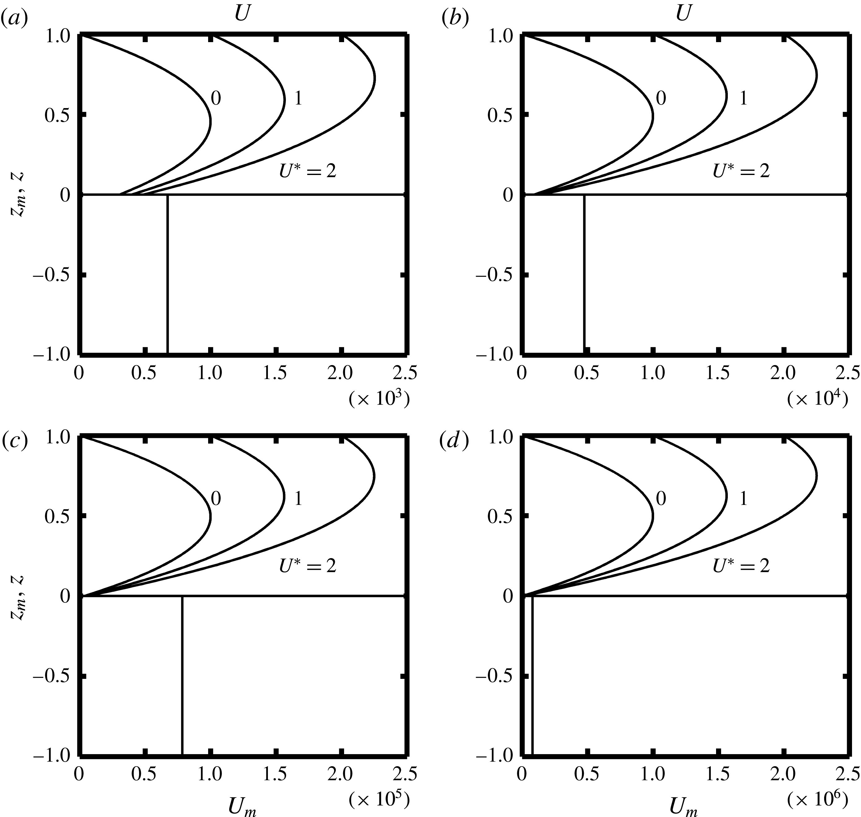
The depth ratio $\hat{d}$ is the dominant parameter for the stability problem of a fluid layer overlying a porous layer. Several typical values of depth ratio $\hat{d}$ are taken into consideration and the other parameters used in the calculations are given by $\unicode[STIX]{x1D6FF}=10^{-3}$ , $\unicode[STIX]{x1D712}=0.3$ and $\unicode[STIX]{x1D6FC}=0.1$ , which are practical properties of many porous materials (Straughan Reference Straughan2002). Before proceeding to the stability analysis, we first pay attention to the variation of basic flows with depth ratio as illustrated in figure 1(a–d) for the four assigned values of $\hat{d}$ with three typical speed ratios of $U^{\ast }$ . It is obvious that the flow velocity $U_{m}$ in the porous layer is independent of $U^{\ast }$ and significantly less than the magnitude of $U$ in the fluid layer. The velocity jump at the interface due to the Beavers–Joseph boundary condition is significant in the case of $\hat{d}=0.1$ , as shown in figure 1(a), in which $U_{m}=6.72\times 10^{-4}$ jumps to $U=0.306$ , 0.397 and 0.485 for $U^{\ast }=0$ , 1 and 2, respectively. This result also indicates a large interfacial shear stress at the interface according to (2.7c ). However, as the depth ratio increases, the fluid-layer velocity $U$ at the interface decreases quickly and the porous-layer velocity $U_{m}$ diminishes simultaneously. For example, in figure 1(c) for the case of $\hat{d}=1.0$ , the velocity at the interface jumps from $U_{m}=7.84\times 10^{-6}$ to $U=3.88\times 10^{-2}$ , $4.87\times 10^{-2}$ and $5.86\times 10^{-2}$ for $U^{\ast }=0$ , 1 and 2, respectively. As a result, the fluid-layer velocity at the interface approaches zero with increasing $\hat{d}$ and the effect of interfacial shear stress at the interface decays gradually. For the case of $\hat{d}=10$ , as shown in figure 1(d), the velocity $U_{m}$ reduces to a negligible value of $7.98\times 10^{-8}$ and the base flow in the fluid layer is almost the same as the PPC flow in a single fluid layer.

Figure 1.

The basic states of dimensionless velocities $U$ and $U_{m}$ in the fluid and porous layers for four assigned depth ratios with three typical values of $U^{\ast }$ : (a) $\hat{d}=0.1$ , (b) $\hat{d}=0.4$ , (c) $\hat{d}=1.0$ and (d) $\hat{d}=10$ .

Figure 2.

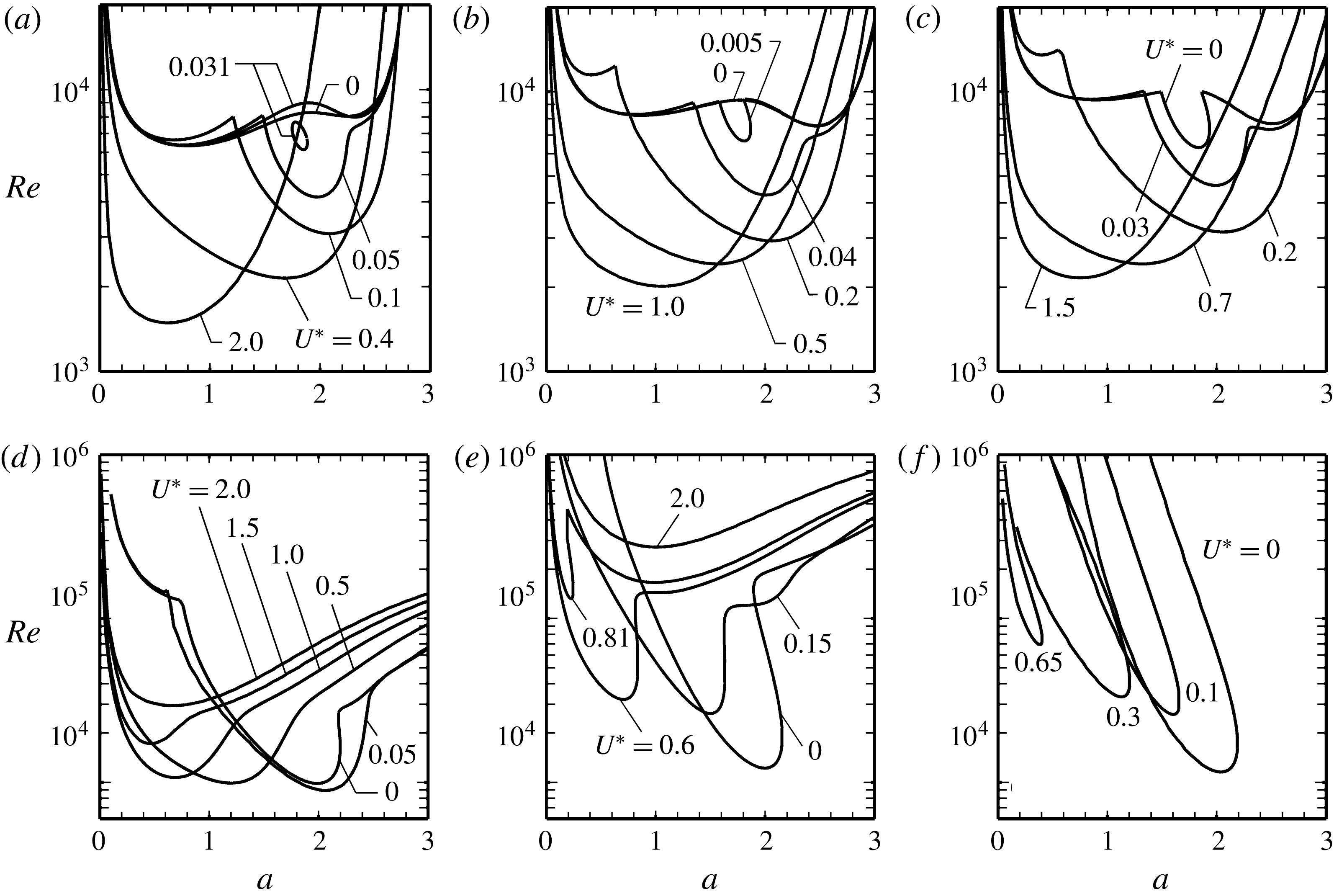
The variations of neutral curve with velocity ratio $U^{\ast }$ at several assigned values of depth ratio: (a) $\hat{d}=0.1$ , (b) $\hat{d}=0.12$ , (c) $\hat{d}=0.13$ , (d) $\hat{d}=0.4$ , (e) $\hat{d}=1.0$ and (f) $\hat{d}=10$ .

Figure 3.

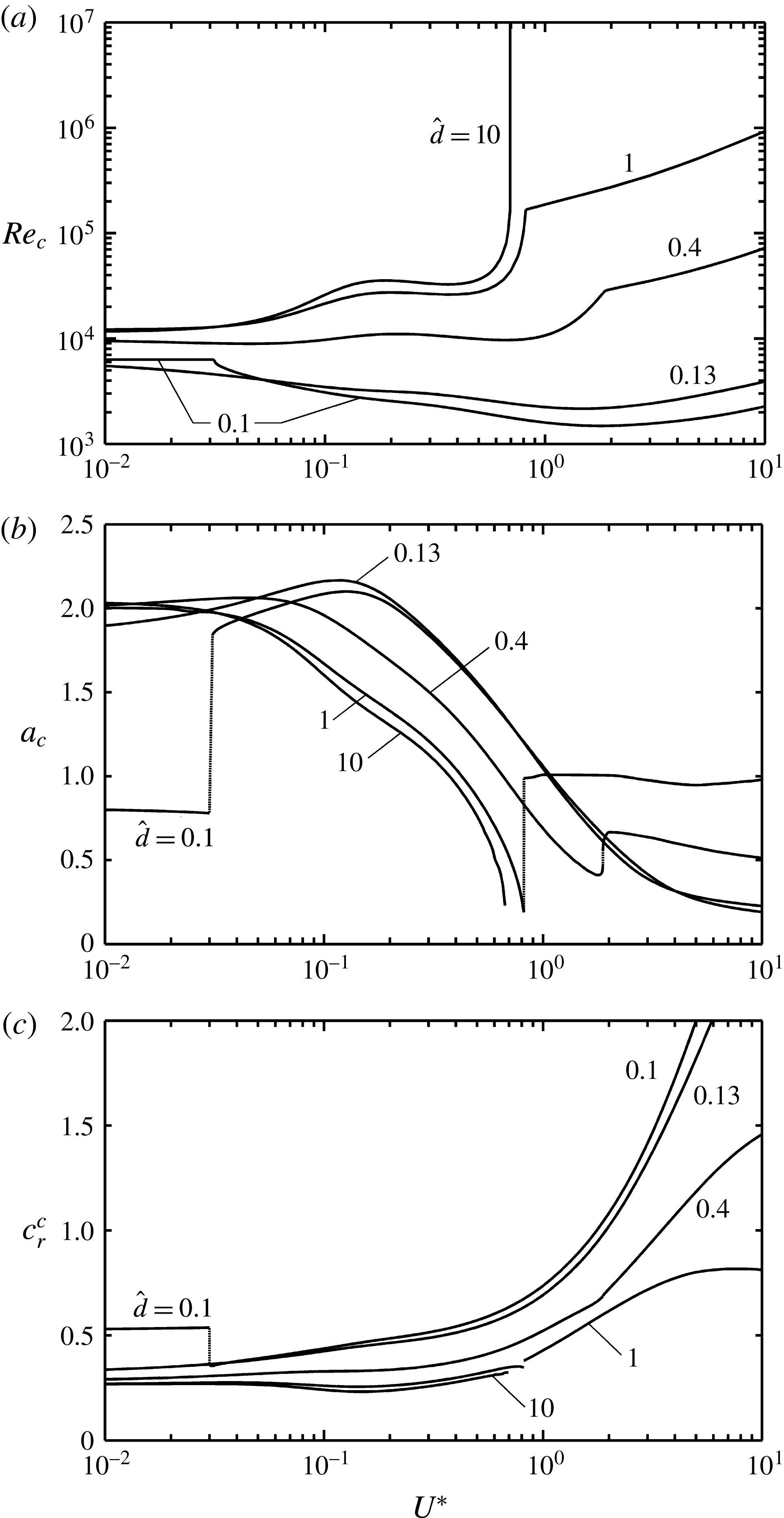
The variations of (a) critical Reynolds number $Re_{c}$ , (b) critical wavenumber $a_{c}$ and (c) critical phase velocity $c_{r}^{c}$ ; with $U^{\ast }$ for several assigned values of depth ratio  $\hat{d}$ .

For the flow instability behaviours, we first consider the case of $\hat{d}=0.1$ . It has been found in the work of Chang et al. (Reference Chang, Chen and Straughan2006) that the neutral curves display a bi-modal structure as shown in figure 2(a) for the case of $U^{\ast }=0$ in which the component of Couette flow is absent. The dominant mode of instability is determined by the left minimum at lower wavenumber, which is the so-called porous-layer mode at which the onset of instability occurs within both the fluid and porous layers and that is primarily dominated by the porous medium. The right minimum at higher wavenumber is named the odd-fluid-layer mode due to the odd-symmetry profile of streamfunction $\unicode[STIX]{x1D719}$ with respect to the centreline of fluid layer (Chang et al. Reference Chang, Chen and Straughan2006). Once the Couette flow begins to exert its effect on the system, it is found that both the minima are without any significant variation initially while a small loop appears abruptly below the neutral curve of the two minima when the component of Couette flow is large enough, as shown in the case of $U^{\ast }=0.031$ . The onset of instability is then dominated by this mode and the loop grows rapidly with increasing the speed ratio and eventually merges with the upper neutral curve, forming a tri-modal structure as shown in the case of $U^{\ast }=0.05$ . Obviously, the third instability mode results from the enhancement of shear in the fluid layer due to the imposed Couette flow, which is named the even-fluid-layer mode because of its even-symmetry eigenfunction of $\unicode[STIX]{x1D719}$ in the fluid layer. The shear mode dips lower gradually with increasing the speed ratio $U^{\ast }$ while the other two modes rise, recede and disappear eventually. The corresponding variations of the critical Reynolds number $Re_{c}$ , wavenumber $a_{c}$ and phase velocity $c_{r}^{c}$ are shown in figures 3(a)–3(c), respectively. As illustrated in figure 3(a) for the case of $\hat{d}=0.1$ , the variation of neutral curves causes the critical Reynolds number to decrease suddenly at $U^{\ast }=0.031$ due to the shift of the instability mode, and then to reduce gradually with increasing $U^{\ast }$ . Such stability behaviours are quite different from those of pure Couette and PPC flows in a single fluid layer. It is well known that the Couette flow in a single fluid layer is unconditionally stable for small disturbances (cf. Drazin & Reid Reference Drazin and Reid1985). For the PPC flow in a fluid layer, the work of Potter (Reference Potter1966) had found that the presence of Couette flow produces a strong stabilizing effect on the Poiseuille flow. However, the present results show that the imposed Couette flow may destabilize the Poiseuille flow significantly under small depth ratio conditions in such a two-layer system. The Couette flow tends to enhance the shear effect of the Poiseuille flow in the fluid layer initially and thus destabilize the base flow. As the speed of upper plate increases further, the flow instability is gradually dominated by the Couette flow. Hence, the critical Reynolds number reaches a minimum near $U^{\ast }=1.79$ and then increases monotonically with increasing $U^{\ast }$ , indicating that the base flow is stabilized by the imposed Couette flow when its magnitude is high enough. The corresponding critical wavenumber $a_{c}$ jumps to a higher value at $U^{\ast }=0.031$ and the critical phase velocity $c_{r}^{c}$ jumps to a lower value simultaneously due to the shift of critical mode. The value of $a_{c}$ increases to a maximum near $U^{\ast }=0.127$ and then decreases gradually, while $c_{r}^{c}$ increases monotonically after the shift of instability mode.

Similar stability characteristics also can be observed in the typical cases of $\hat{d}=0.12$ and 0.13, as shown in 2(b) and 2(c), respectively. In figure 2(b), the right minimum on the bi-modal neutral curve for the case of $U^{\ast }=0$ initially determines the critical mode. The imposed Couette flow triggers the onset of a third mode quickly and forms the tri-modal neutral curve, as seen in the case of $U^{\ast }=0.005$ . The third mode extends and dips down to dominate the onset of instability with increasing $U^{\ast }$ while the other two modes recede gradually. In figure 2(c), the neutral curve is already a tri-modal structure in the absence of Couette flow at $\hat{d}=0.13$ and the middle third mode gives the minimum on the neutral curve. It is apparent that an increase of Couette component enhances the growth of the third mode and destabilizes the flow. Note that the critical wavenumber corresponding to the location of the minimum of $Re$ at first moves to the right on the $(a,Re)$ -plane and then moves to the left gradually to form the so-called ‘long-wave’ instability mode. The variations of $Re_{c}$ and $a_{c}$ with $U^{\ast }$ are illustrated respectively in 3(a) and 3(b) for the typical case of $\hat{d}=0.13$ . It is noted that the results are similar to those of the case $\hat{d}=0.1$ when the third shear mode determines the critical mode and the critical Reynolds number exhibits a minimum near $U^{\ast }=1.48$ . The critical phase velocity $c_{r}^{c}$ increases monotonically with $U^{\ast }$ , as shown in figure 3(c), since the onset of instability is always dominated by the shear mode in this case.

The stability of the present two-layer flow is generally enhanced by increasing the depth ratio, as demonstrated in figure 3(a). Particularly, it is found that the destabilizing effect caused by the component of Couette flow decays gradually as the depth ratio increases. As shown in figure 2(d) for the case $\hat{d}=0.4$ , the lobes of the neutral curve corresponding to both the left porous-layer mode and the right odd-fluid-layer mode disappear and only the even-fluid-layer mode induced by the shear flow in the fluid layer controls the onset of instability. Once the speed ratio $U^{\ast }$ increases, the critical Reynolds number first reduces slightly, as shown in the case of $U^{\ast }=0.05$ , and then the minimum on the neutral curve moves to the left horizontally within a small range of $Re$ until $U^{\ast }\approx 1.0$ , which also can be observed in figure 3(a). 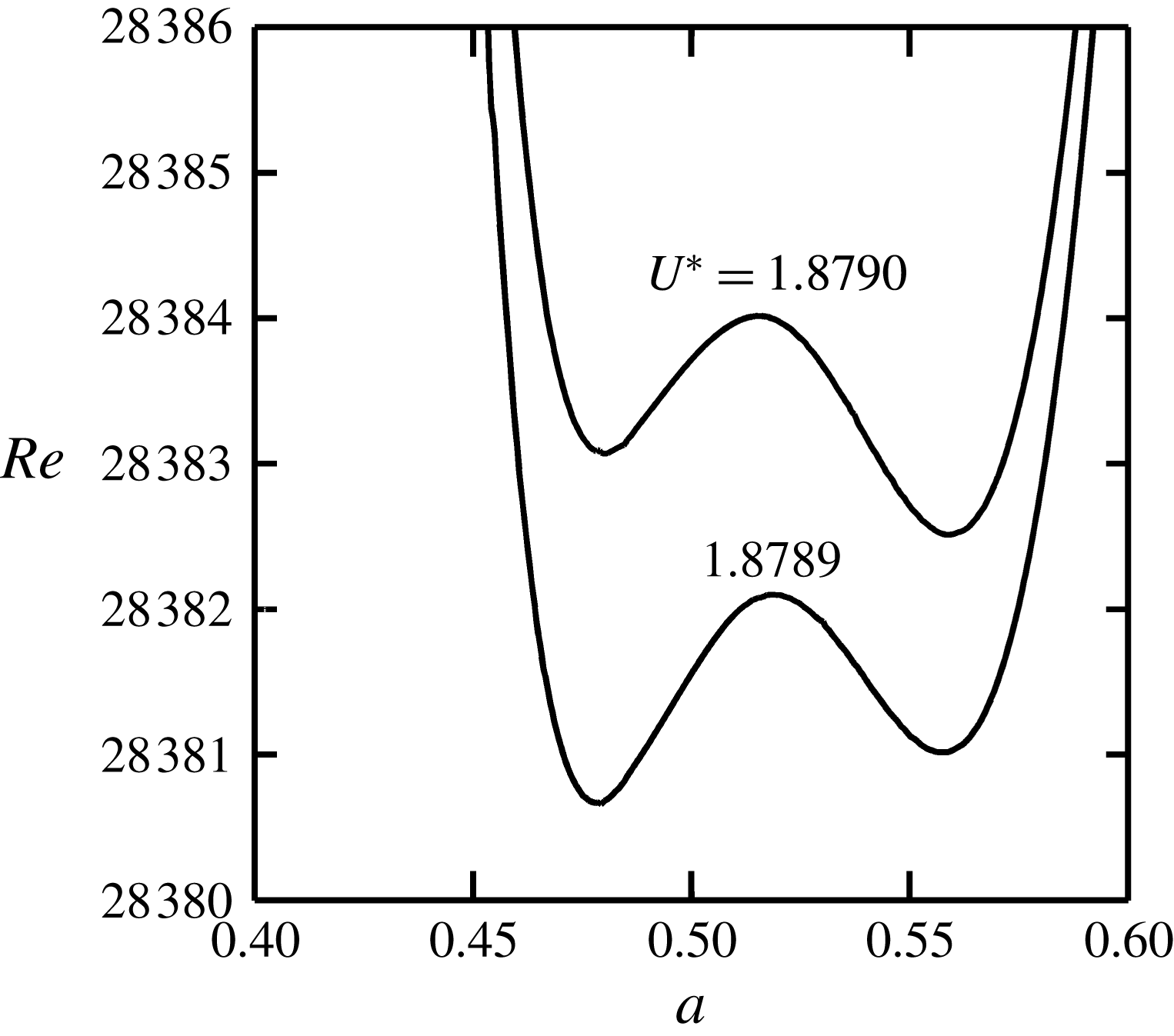The critical Reynolds number begins to rise significantly as $U^{\ast }$ increases further and an instability mode switch occurs within the narrow range of $1.8<U^{\ast }<1.9$ as indicated in figure 3(a), together with a jump of $a_{c}$ and a discontinuity in the slope of $c_{r}^{c}$ , as shown in 3(b) and 3(c), respectively. The shift of instability mode can be observed clearly by the typical neutral curves displayed in figure 4. It is obvious that the neutral curve becomes bi-modal again and the left minimum determines the critical mode at $U^{\ast }=1.8789$ . However, a slight increase in $U^{\ast }$ to 1.879 makes the neutral curve rise and the right minimum becomes lower than the left one to dominate the instability. The switch of instability mode causes the $a_{c}$ jump from 0.48 to 0.57. The bi-modal neutral curve occurs only within a limited range of $U^{\ast }$ and the left mode recedes quickly after the occurrence of the mode switch. The characteristics of the right critical mode will be discussed later by examining the magnitude of the eigenfunction and the pattern of the streamfunction of the small disturbance.

Figure 4.

The neutral curves of two assigned values of $U^{\ast }$ at $\hat{d}=0.4$ , illustrating the shift of the instability mode.

The destabilizing effect of the Couette flow on the PPC flow as the Couette component increases from zero totally vanishes when the depth ratio is large enough. On the contrary, the presence of Couette flow begins to exhibit a stabilizing effect as shown in figure 2(e) for the case $\hat{d}=1.0$ . The neutral curves rise and recede to the left with increasing $U^{\ast }$ . Especially, the phenomenon regarding the shift of the instability mode when the velocity ratio $U^{\ast }$ exceeds a certain critical value is more pronounced as $\hat{d}$ increases. One can see that a local minimum gradually appears on the right branch to form a bi-modal structure on the neutral curve. Once the velocity ratio $U^{\ast }$ is greater than 0.817 in this typical case, the critical mode shifts abruptly from the left long-wave mode to the right one at higher wavenumber. The long-wave instability mode disappears eventually as illustrated in the neutral curve of $U^{\ast }=2.0$ and the right mode totally controls the onset of instability. The corresponding variation of $a_{c}$ , as displayed in figure 3(b), shows a more significant discontinuity due to the shift of the instability mode at $U^{\ast }\approx 0.817$ . Simultaneously, the critical phase velocity $c_{r}^{c}$ also jumps to a higher value as illustrated in figure 3(c).

Figure 5.

The normalized eigenfunctions $\unicode[STIX]{x1D719}$ , $\unicode[STIX]{x1D719}_{m}$ and the corresponding patterns of the streamfunction $\unicode[STIX]{x1D713}$ for the four typical values of $U^{\ast }$ at $\hat{d}=0.1$ : (a) $U^{\ast }=0$ , (b) $U^{\ast }=0.031$ , (c)  $U^{\ast }=0.4$ and (d) $U^{\ast }=2.0$ .

The typical case $\hat{d}=10$ is taken into consideration and the results indicate that the influence of porous layer could be ignored when the thickness of the fluid layer is much greater than that of porous layer. The variations of the neutral curves in figure 2(f) and the critical Reynolds number with $U^{\ast }$ in figure 3(a) are exactly the same as the results found by Potter (Reference Potter1966) that concluded that the superimposed Couette flow has a strong stabilizing effect on the Poiseuille flow. Besides, the critical Reynolds number and wavenumber for $U^{\ast }=0$ are respectively 11 586.05 and 2.0376, which are also in good agreement with the results of the Orr–Sommerfeld equation in the common Poiseuille channel flow with $Re_{c}=11\,544.44$ and $a_{c}=2.0411$ (Drazin & Reid Reference Drazin and Reid1985) based on the channel height as the characteristic length. The comparison is more excellent for higher $\hat{d}$ which verifies the accuracy of the present numerical algorithm. As illustrated in figure 3(a), the critical Reynolds number approaches infinity near $U^{\ast }\approx 0.7$ which is the so-called cutoff velocity and the critical wavenumber approaches zero. Once the speed of the moving boundary is greater than the cutoff velocity, the PPC flow becomes unconditional stable for all infinitesimal disturbances. It is noted that in the range of $0.2<U^{\ast }<0.4$ , there exists a local minimum which indicates the flow becomes more unstable with increased Couette flow. Potter observed that this effect occurs when $U^{\ast }$ is approximately equal to the travelling phase velocity $c_{r}$ . A more detailed explanation for this phenomenon was given in the study of Özgen et al. (Reference Özgen, Dursunkaya and Ebrinc2007), in which they proposed that this stability behaviour is related to the evolution of $U^{\ast }$ with the phase velocity and the exchange of energy between the perturbation and the base flow due to the change in the location of the critical layer. The critical layer is defined as the location where both the phase velocity and the base flow velocity are equal. It plays an important role in transferring the energy of the base flow to the disturbances. They observed that the critical layer is very close to the moving wall in the range of $0.2<U^{\ast }<0.25$ and thus produces a destabilizing effect. The present results show that the critical velocity ratio of $U^{\ast }$ corresponding to the shift of instability mode from the long-wave mode to the mode at higher wavenumber decreases gradually with increasing $\hat{d}$ . Once $\hat{d}$ is large enough, the phenomenon of mode switch vanishes and only the neutral curve corresponding to the long-wave instability mode may appear on the $(a,Re)$ plane. The instability behaviours are in good agreement with those studies for PPC flow in a single fluid layer.

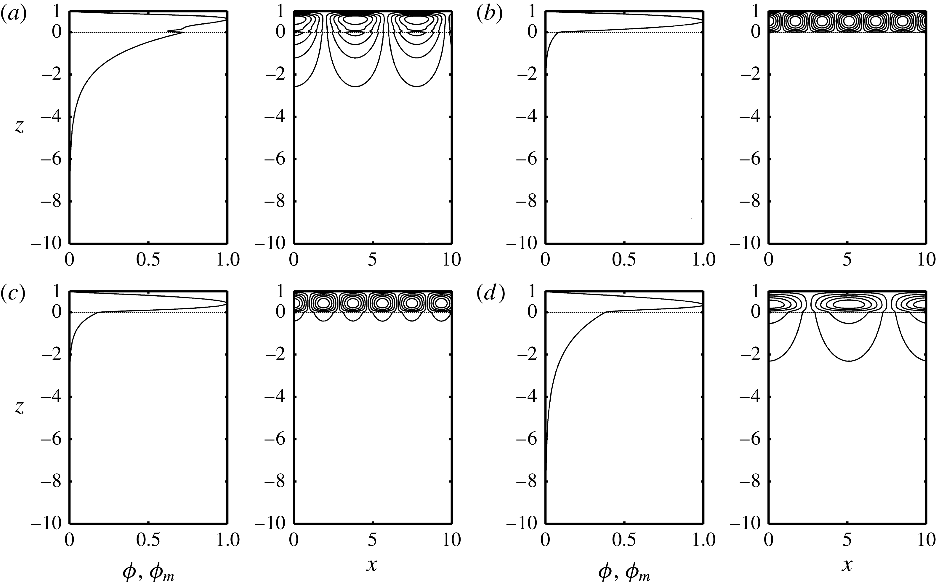
The characteristics of the instability modes can be explored further by observing the profiles of the normalized eigenfunctions $\unicode[STIX]{x1D719}$ and $\unicode[STIX]{x1D719}_{m}$ , and the corresponding patterns of streamfunctions $\unicode[STIX]{x1D713}$ and $\unicode[STIX]{x1D713}_{m}$ at the critical states, as displayed in figure 5(a–d) for the four typical cases of $U^{\ast }$ at $\hat{d}=0.1$ . It is noted that both the vertical $z$ -axis and horizontal $x$ -axis are scaled by the thickness of the fluid layer. Thus, the fluid layer is always indicated in the range of $z\in (0,1)$ and the range of porous layer depends on the depth ratio in the following similar figures. In figure 5(a), the magnitude of streamfunction penetrates into the porous layer for the porous-layer mode and the corresponding flow pattern occupies both the fluid and porous layers at $U^{\ast }=0$ . Above the interface, the magnitude of $\unicode[STIX]{x1D719}$ first decreases slightly with increasing $z$ , reaches a local minimum and then increases gradually to the maximum. Such a variation causes the occurrence of a small vortex motion on the streamfunction pattern of the small disturbances which occupies the thin region across the interface. It has been pointed out by Lyubimova et al. (Reference Lyubimova, Lyubimov, Baydina, Kolchanova and Tsiberkin2016) that the rapid reduction of tangential velocity at the interface may result in flow instability similar to the Kelvin–Helmholtz instability. Obviously, the small vortex motion at the interface is induced by the significant velocity jump of the basic state, as illustrated in figure 1(a). The onset of instability shifts to the fluid-layer mode at $U^{\ast }=0.031$ , in which the streamfunction pattern concentrates mainly within the fluid layer with shorter wavelength. The magnitude of $\unicode[STIX]{x1D719}$ then gradually penetrates into the porous layer again with increasing $U^{\ast }$ as shown in figure 5(b–d). Similar variations of the streamfunction pattern can also be observed for the cases of $\hat{d}=0.12$ and 0.13. 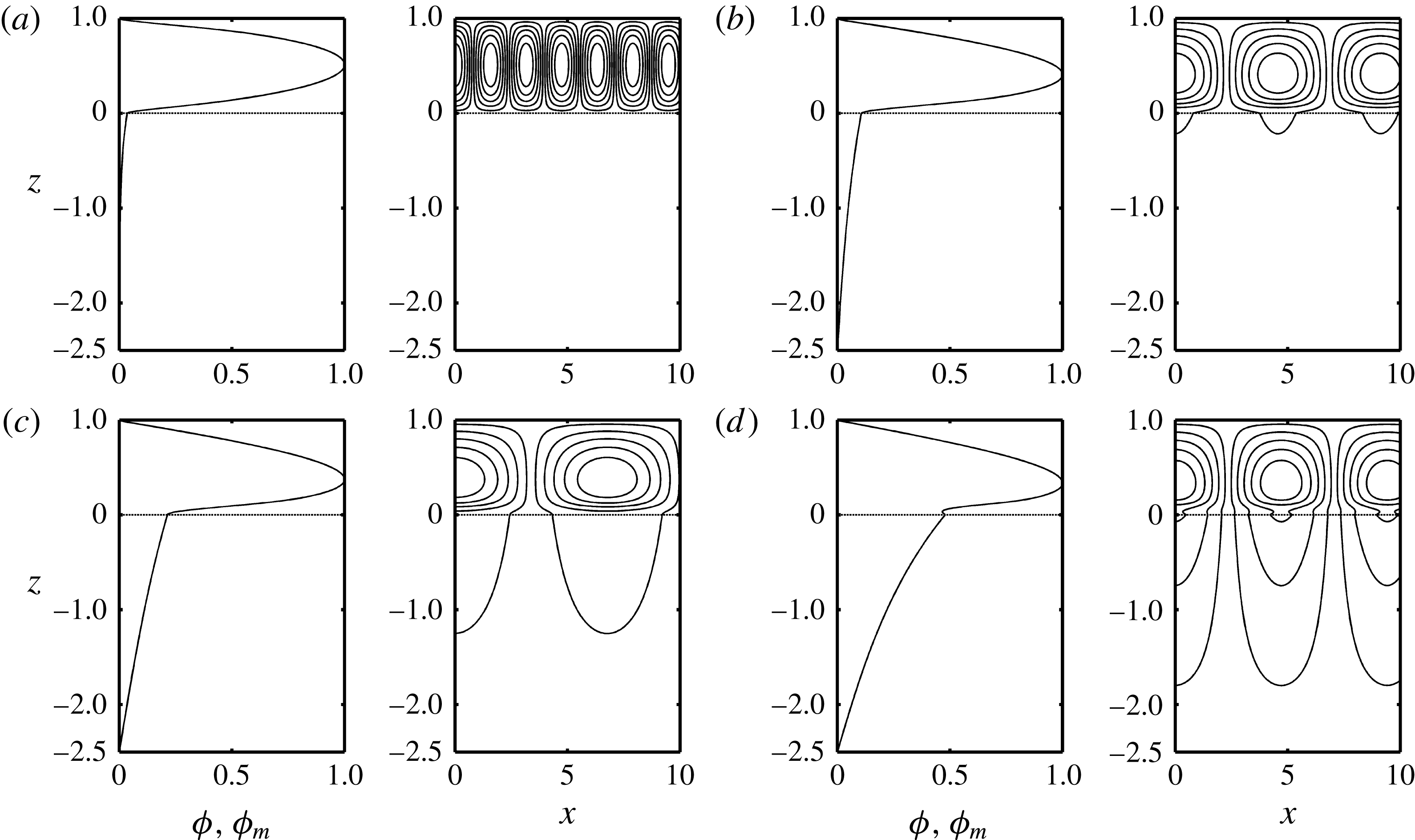For the case of $\hat{d}=0.4$ , the fluid-layer mode is predominant at $U^{\ast }=0$ and the pattern is within the fluid layer only, as illustrated in figure 6(a). The pattern of the streamfunction gradually penetrates into the porous layer and the wavelength increases simultaneously, as shown in figures 6(b) and 6(c) for $U^{\ast }=1.0$ and 1.5, respectively. Once the speed ratio $U^{\ast }$ increases to 1.879, the Couette flow gradually prevails over the Poiseuille flow and induces the shift of the instability mode as shown in figure 4. Obviously, the left critical mode corresponds to the fluid-layer mode such that the magnitude of the streamfunction is mainly within the fluid layer, while the right one corresponds to the porous-layer mode because the unstable wave penetrates into the porous layer again, as shown in figure 6(d) for the case of $U^{\ast }=2.0$ . A small and weak cell on the interface similar to that in figure 5(a) is also observed. As shown in figure 1(a–d), the effect of the horizontal velocity jump reduces rapidly with increasing $\hat{d}$ . Hence, the vortex motion at the interface induced by the velocity jump decays quickly in the porous-layer mode. The critical wavelength is shortened and the porous-layer mode becomes dominant after the shift of the instability mode. 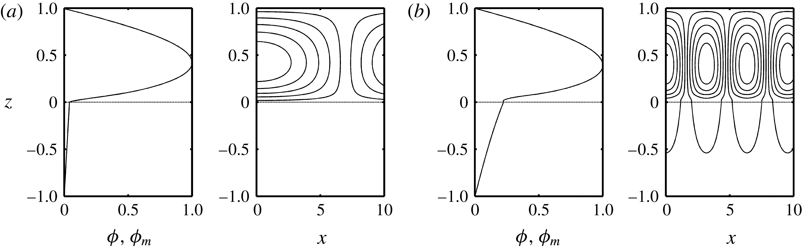This phenomenon for the instability mode switch is more apparent for the case of $\hat{d}=1.0$ as $U^{\ast }$ near 0.817. The results are shown in figure 7(a,b) for the typical cases of $U^{\ast }=0.81$ and 0.85. 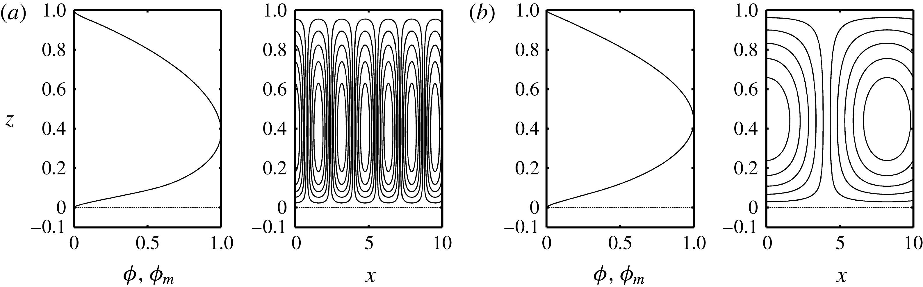One can see that the magnitude and pattern of $\unicode[STIX]{x1D719}$ penetrate into the porous layer after the occurrence of mode switch as the effect of Couette flow becomes pronounced in the PPC flow. Note that the small vortex motion in the porous-layer mode at the interface totally vanishes in figure 7(b). However, once the influence of porous layer is negligible at higher depth ratio, for example, $\hat{d}=10$ , the behaviour of the instability mode switch from the fluid-layer mode to the porous-layer mode at high velocity ratio vanishes eventually. Only the fluid-layer modes are observed as shown in figure 8(a,b) for the two typical cases of $U^{\ast }=0.3$ and 0.65 at $\hat{d}=10$ .

Figure 6.

The normalized eigenfunctions $\unicode[STIX]{x1D719}$ , $\unicode[STIX]{x1D719}_{m}$ and the corresponding patterns of the streamfunction $\unicode[STIX]{x1D713}$ for the four typical values of $U^{\ast }$ at $\hat{d}=0.4$ : (a) $U^{\ast }=0$ , (b) $U^{\ast }=1.0$ , (c)  $U^{\ast }=1.5$ and (d) $U^{\ast }=2.0$ .

Figure 7.

The normalized eigenfunctions $\unicode[STIX]{x1D719}$ , $\unicode[STIX]{x1D719}_{m}$ and the corresponding patterns of streamfunction $\unicode[STIX]{x1D713}$ for the two typical values of $U^{\ast }$ at $\hat{d}=1.0$ : (a) $U^{\ast }=0.81$ , (b) $U^{\ast }=0.85$ .

Figure 8.

The normalized eigenfunctions $\unicode[STIX]{x1D719}$ , $\unicode[STIX]{x1D719}_{m}$ and the corresponding patterns of streamfunction $\unicode[STIX]{x1D713}$ for the two typical values of $U^{\ast }$ at $\hat{d}=10$ : (a) $U^{\ast }=0.3$ , (b) $U^{\ast }=0.65$ .

3.2 The stability of plane Couette flow

It is well known that the Couette flow in a horizontal fluid layer is unconditionally stable with respect to small disturbances. Since the superimposed Couette flow may destabilize the Poiseuille flow in the present two-layer system, it is interesting to explore whether the pure Couette flow may become conditionally stable due to the existence of the porous layer. It is noted that there is no base flow in the porous layer, as indicated by (2.34). A velocity jump at the interface $z=0$ due to the Beavers–Joseph boundary condition may possibly induce the occurrence of flow instability. From (2.33), it is obvious that the fluid velocity at the interface depends on the Darcy number $\unicode[STIX]{x1D6FF}$ , Beavers–Joseph constant $\unicode[STIX]{x1D6FC}$ and the depth ratio $\hat{d}$ . For the present assigned values of $\unicode[STIX]{x1D6FF}$ and $\unicode[STIX]{x1D6FC}$ , the fluid velocity at the interface is only 9.1 % of the upper plate velocity for the case $\hat{d}=0.1$ . 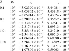This velocity ratio decreases with increasing $\hat{d}$ which indicates the significance of the velocity jump at the interface decreases gradually. Because the tangential velocity jump at the interface is small even though at low depth ratio, it is to be expected that the Couette flow is still always stable. The corresponding linear stability problem has been solved numerically and the results indeed reveal that the pure Couette flow in this two-layer system is still an unconditionally stable flow. Table 1 lists the leading eigenvalues at different Reynolds numbers for several assigned depth ratios. 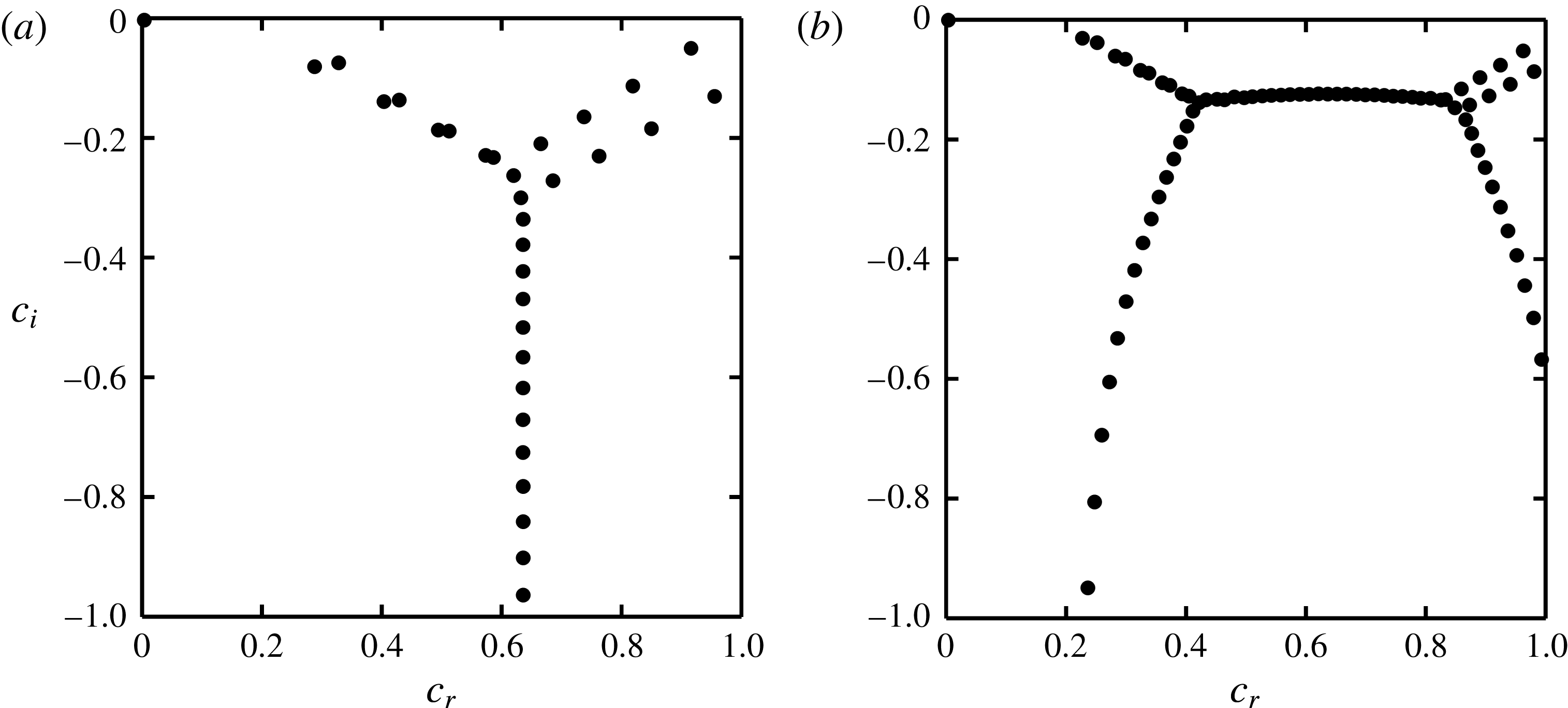It is found that no matter how large the Reynolds number is, the growth rate represented by the imaginary part of the eigenvalue $c$ , $c_{i}$ , is always negative. Figures 9(a) and 9(b) illustrate the spectrum of the typical case of $\hat{d}=0.1$ at $Re=10^{4}$ and $10^{5}$ , respectively. One can see that the value of $c_{i}$ is closer to the neutral state (i.e. $c_{i}=0$ ) with increasing $Re$ . However, it never changes sign to become positive in any the cases considered here.

Table 1.

For pure Couette flow, the leading eigenvalues with largest imaginary parts with respect to $Re$ for several assigned values of $\hat{d}$ at $a=1.0$ .

Figure 9.

The spectra of the eigenvalues at $a=1.0$ with $\hat{d}=0.1$ . (a) $Re=10^{4}$ and (b)  $Re=10^{5}$ .