2 Experiments and Conditional Average Treatment Effects

We follow a large prior literature and formalize the estimation of heterogeneous effects using potential outcome notation (Holland Reference Holland1986; Green and Kern Reference Green and Kern2012; Imai and Ratkovic Reference Imai and Ratkovic2013) and also borrow some notation from recent work on the analysis of conjoint experiments (Hainmueller, Hopkins, and Yamamoto Reference Hainmueller, Hopkins and Yamamoto2014). Suppose that we have a sample of ${\mathcal{N}}$ , $(i=1,\ldots ,N)$ individuals from a population ${\mathcal{P}}$ . We suppose that there are $C$ $(c=1,2,\ldots ,C)$ factors in the experiment and in each of the factors participants are randomly assigned to one of $K_{c}$ conditions and that there is also a control condition. Participant $i$ ’s condition will be given by $\boldsymbol{T}_{i}=(T_{i,1},T_{i,2},\ldots ,T_{i,C})$ if assigned to a treatment condition and otherwise $T_{i}=0$ . We will denote respondent $i$ ’s response to condition $\boldsymbol{T}_{i}$ with the potential outcome $Y_{i}(\boldsymbol{T}_{i})$ .Footnote ¹ We will analyze dichotomous dependent variables, though the ensemble methods generalize easily to continuous or other dependent variables.

To measure the effect of an intervention for the entire population of interest, scholars commonly report an Average Treatment Effect (ATE) across two conditions. For simplicity, we will compare the effect of some treatment condition $\boldsymbol{T}_{i}$ to the control condition $T_{i}=0$ , though comparisons of any two treatments are possible. We will write the ATE as,

(1) $$\begin{eqnarray}\displaystyle \unicode[STIX]{x1D719}(\boldsymbol{T})=E[Y(\boldsymbol{T})-Y(0)]. & & \displaystyle\end{eqnarray}$$

Randomly assigning participants to arms of the treatment ensures that the $\unicode[STIX]{x1D719}(\boldsymbol{T})$ is identified, which is commonly estimated with a difference in means across conditions.

The ATE measures the effect of the intervention over the entire population, but to measure how treatment effects vary across respondent characteristics we will estimate a conditional average treatment effect (CATE) (Imai and Strauss Reference Imai and Strauss2011; Green and Kern Reference Green and Kern2012; Imai and Ratkovic Reference Imai and Ratkovic2013). The CATE, measures the ATE for respondents who share a set of characteristics. To formalize this definition, suppose that for each respondent $i$ we collect $J$ covariates $(j=1,2,\ldots ,J)$ , $\boldsymbol{X}_{i}=(X_{i1},X_{i2},\ldots ,X_{iJ})$ , with values of the covariates collected in the set ${\mathcal{X}}$ . We can then define the CATE for covariate profile $\boldsymbol{x}\in {\mathcal{X}}$ , and treatment arm $\boldsymbol{T}$ as $\unicode[STIX]{x1D719}(\boldsymbol{T},\boldsymbol{x})$ ,

(2) $$\begin{eqnarray}\displaystyle \unicode[STIX]{x1D719}(\boldsymbol{T},\boldsymbol{x})=\text{E}[Y(\boldsymbol{T})-Y(0)|\boldsymbol{X}=\boldsymbol{x}]. & & \displaystyle\end{eqnarray}$$

A treatment effect is heterogeneous if the value of Equation 2 varies as we consider different strata of participants. As before, random assignment to treatment conditions is sufficient to identify the CATE.

The CATE measures the effect for respondents who share identical values of all $J$ covariates. We may be interested, however, in how responses to the treatment effect vary across a subset of covariates, a single covariate, or a single factor. Suppose that we are interested in estimating the marginal effect of a subset of covariates $\boldsymbol{X}_{S}=(X_{s_{1}},X_{s_{2}},\ldots ,X_{S})$ . Define the marginal conditional average treatment effect (MCATE) for covariates $\boldsymbol{X}_{S}$ and treatment conditions $\boldsymbol{T}$ , $\unicode[STIX]{x1D719}(\boldsymbol{T},\boldsymbol{x}_{S})$ ,

(3) $$\begin{eqnarray}\displaystyle \unicode[STIX]{x1D719}(\boldsymbol{T},\boldsymbol{x}_{S}) & = & \displaystyle \int \unicode[STIX]{x1D719}(\boldsymbol{T},(X_{1},X_{2},\ldots ,\boldsymbol{X}_{S}=\boldsymbol{x}_{S},\ldots ,X_{J}))dF_{\boldsymbol{X}_{-S}|\boldsymbol{X}_{S}=\boldsymbol{x}_{S}}\nonumber\\ \displaystyle & = & \displaystyle \int E[Y(\boldsymbol{T})-Y(0)|(X_{1},X_{2},\ldots ,\boldsymbol{X}_{S}=\boldsymbol{x}_{S},\ldots ,X_{J})]dF_{\boldsymbol{X}_{-S}|\boldsymbol{X}_{S}=\boldsymbol{x}_{S}}.\end{eqnarray}$$

And finally we define the marginal average treatment effect (MATE) for factor $c$ as $\unicode[STIX]{x1D719}(T_{c}=k)$ as

(4) $$\begin{eqnarray}\displaystyle \unicode[STIX]{x1D719}(T_{c}=k) & = & \displaystyle \int \unicode[STIX]{x1D719}(\boldsymbol{T})\,dF_{\boldsymbol{T}_{-c}|T_{c}=k}\nonumber\\ \displaystyle & = & \displaystyle \int E[Y(\boldsymbol{T})-Y(0)]\,dF_{\boldsymbol{T}_{-c}|T_{c}=k}\end{eqnarray}$$

where $F_{\boldsymbol{X}_{-S}|\boldsymbol{X}_{S}=\boldsymbol{x}_{S}}$ is the joint distribution of the covariates $\boldsymbol{X}_{-S}$ , given that $\boldsymbol{X}_{S}=\boldsymbol{x}_{S}$ and $dF_{\boldsymbol{T}_{-c}|T_{c}=k}$ . In words, Equation 3 shows that MCATEs are averages of CATEs, where the value of the covariate of interest is fixed and $F_{\boldsymbol{X}_{-S}|\boldsymbol{X}_{S}=\boldsymbol{x}_{S}}$ is used to weight other covariate profiles and Equation 4 shows that MATEs are averages of ATEs and $F_{\boldsymbol{T}_{-c}|T_{c}=k}$ is used to weight the treatment profiles.

This notation corresponds to well-known quantities of interest scholars commonly compute. For example, when applying a parametric bootstrap, such as Clarify, it is common to set variables other than the covariate of interest to the sample means to estimate marginal effects (King, Tomz and Wittenberg Reference King, Tomz and Wittenberg2000). This is equivalent to $F_{\boldsymbol{X}_{-S}|\boldsymbol{X}_{S}=\boldsymbol{x}_{S}}$ to place all probability on the sample means and zero elsewhere. It may be possible to estimate the joint distribution, facilitating extrapolation from the sample population to some other sample or population (Hartman et al. Reference Hartman, Grieve, Ramshai and Sekhon2012). And finally, we may average over all other possible covariate values—for discrete random variables—or a grid of values for continuous random variables. This is equivalent to setting $F_{\boldsymbol{X}_{-S}|\boldsymbol{X}_{S}=\boldsymbol{x}_{S}}$ to a uniform distribution.

3 Estimation of Heterogeneous Treatment Effects with a Weighted Ensemble of Methods

When there are a large number of observations in each condition and participants who share the same set of covariates, reliable estimation of ATEs, CATEs, MATEs, and MCATEs is straightforward. The random assignment of participants to treatments ensures that a difference in means across treatment arms will reliably estimate the ATE and a difference in means across arms among respondents with the same set of covariates provides an accurate estimate of CATEs and MCATEs. With a large number of participants, the differences computed with naïve differences in means will tend to reflect systematic differences (Gelman, Hill, and Yajima Reference Gelman, Hill and Yajima2012).

But for more heterogeneous treatments with a large number of conditions, or covariates that have few observations who share the exact same covariates, a simple difference in means will be a less reliable estimate of the effect of treatments. When the sample size is relatively small, naïve differences will be likely to reflect random variation in the sample, rather than systematic differences in the underlying methods because there will be few observations who share the exact same characteristics. This renders ineffective the usual method for estimating heterogeneous treatment effects: computing a difference in means for observations with the same covariate value. It also makes simple comparisons of different levels of high-dimensional treatments highly problematic.

The goal in estimating heterogeneous effects is to separate the systematic responses from differences solely due to chance of the random assignment. Several new methods provide novel ways to identify the systematic effects. Each method $m$ estimates the response surface for any treatment $k$ and covariates $\boldsymbol{x}$ ,

(5) $$\begin{eqnarray}\displaystyle g_{m}(\boldsymbol{T},\boldsymbol{x}) & = & \displaystyle E[Y|\boldsymbol{T},\boldsymbol{x}]\end{eqnarray}$$

and quantities of interest are computed by taking differences across the response surfaces.

To estimate Equation 5 each of the methods vary necessary and consequential assumptions about how treatment assignment and covariates alter the response surface. For example, one approach to estimating heterogeneous treatment effects is to use regression trees (Imai and Strauss Reference Imai and Strauss2011) and Bayesian Additive Regression Trees (BART) to estimate CATEs and MCATEs (Chipman, George, and McCulloch Reference Chipman, George and McCulloch2010; Green and Kern Reference Green and Kern2012). The trees subdivide the data repeatedly, developing decision rules to split the data to make more accurate predictions. An ensemble of the trees is then used to model the response surface and estimate the heterogeneous effects. Other methods start from a more familiar regression framework and then use data and assumptions to identify systematic differences. For example, LASSO methods use a penalty to shrink some coefficients to zero (Hastie, Tibshirani and Friedman Reference Hastie, Tibshirani and Friedman2001; Athey and Imbens Reference Athey and Imbens2015). Imai and Ratkovic (Reference Imai and Ratkovic2013) extend and generalize LASSO, introducing a model that has two different penalties—one for covariates and another for variation in treatment effects. A different, though related, approach is to impose a model that shrinks the coefficients to a common mean, allowing only the strongest coefficients to take on distinct values (Gelman et al. Reference Gelman, Jakulin, Pittau and Su2008). Hainmueller and Hazlett (Reference Hainmueller and Hazlett2013) extend this idea further and include a much more flexible modeling approach with Kernel Regularized Least Squares (KRLS) and prove useful statistical properties of the algorithm.Footnote ² And still other methods balance between the two types of smoothing. Elastic Net is a method that includes penalties that both shrink to zero and shrink to a common mean, with the weight attached to each penalty determined by a parameter $\unicode[STIX]{x1D6FC}$ , $0<\unicode[STIX]{x1D6FC}<1$ (Hastie, Tibshirani and Friedman Reference Hastie, Tibshirani and Friedman2001).

Each of the methods have been shown to perform well on important political science examples. Yet, knowing the ideal method to apply in any one experiment requires knowledge about the data generating process that assumes the heterogeneous effect sizes are known—exactly what we set out to estimate. For example, Imai and Ratkovic (Reference Imai and Ratkovic2013) impose a sparseness assumption, using a method that identifies a set of treatments and covariates that have no effect on the response surface. In contrast, Hainmueller and Hazlett (Reference Hainmueller and Hazlett2013) assume the estimates are more dense, smoothing many of the coefficient estimates to approximately the same value (Hastie, Tibshirani and Friedman Reference Hastie, Tibshirani and Friedman2001).

The appropriateness of those modeling assumptions will vary across substantive problems. New and diverse methods, then, are essential for estimating accurate heterogeneity in treatment effects. But relying on a single method will result in suboptimal performance across diverse problems. When the assumptions fit the data generation process, the model will perform well, but when the assumptions are a poor fit the method will perform poorly.

In place of using a single method to estimate heterogeneous effects, we argue for a weighted ensemble of estimators. As we show below, we use a weighted ensemble because it tends to attach the greatest weight to the methods that perform best at the task at hand (van der Laan, Polley, and Hubbard Reference van der Laan, Polley and Hubbard2007). Asymptotically ensemble methods will select the best performing methods for a particular problem from the collection of methods (van der Laan, Polley, and Hubbard Reference van der Laan, Polley and Hubbard2007). We show in simulations that in a finite sample ensembles lead to better estimates, as measured by root mean square error. Ensembles are also useful because they can estimate more complex functional forms than the underlying methods. And ensembles make estimates more robust—limiting the possibility that a coding error in any one method could lead to invalid conclusions (Dietterich Reference Dietterich2000).

3.1 Constructing the ensemble via super learning

The ensemble estimator we utilize is a weighted average of heterogeneous treatment effect estimators, where the estimators outof- sample performance will determine the weights. To construct this weighted average, we use the cross validation based methodology super learning introduced in van der Laan, Polley, and Hubbard (Reference van der Laan, Polley and Hubbard2007), a method that we show in the online Appendix is closely related to other ensemble methods (Raftery et al. Reference Raftery, Gneiting, Balabdaoui and Polakowski2005; Montgomery, Hollenbach, and Ward Reference Montgomery, Hollenbach and Ward2012). Ensembles of methods are increasingly used for diverse problems including supervised text classification (Hillard, Purpura and Wilkerson Reference Hillard, Purpura and Wilkerson2008) and prediction (Raftery et al. Reference Raftery, Gneiting, Balabdaoui and Polakowski2005; Montgomery, Hollenbach, and Ward Reference Montgomery, Hollenbach and Ward2012; van der Laan, Polley, and Hubbard Reference van der Laan, Polley and Hubbard2007). Both classification and prediction tasks are closely related to the estimation of heterogeneous treatment effects. In classification and prediction, the goal is to estimate a function such as $g(\boldsymbol{T},\boldsymbol{x})$ , in order to make an out-of-sample estimate about a document or future observation. Heterogeneous treatment effects share a similar goal, but take the difference between response surfaces to estimate the heterogeneous effects. As in classification and prediction, identifying features—covariates and treatment assignments—that systematically affect the response surface will improve our estimates of the quantities of interest.

To construct the ensemble, assume we include $M$ models $(m=1,2,\ldots ,M)$ for estimating heterogeneous effects. For each method $m$ we will define its estimate of $E[Y(\boldsymbol{T})|\boldsymbol{T}]=g_{m}(\boldsymbol{T})$ and $E[Y(\boldsymbol{T})|\boldsymbol{T},\boldsymbol{x}]=g_{m}(\boldsymbol{T},\boldsymbol{x})$ . Along with the $M$ models, we will suppose that we have a set of weights attached to each of the models $\boldsymbol{w}=(w_{1},w_{2},\ldots ,w_{M})$ . We will assume that all weights are greater than or equal to zero ( $w_{m}\geqslant 0$ for all $m$ ) and the weights sum to 1 ( $\sum _{m=1}^{M}w_{m}=1$ ).

With the weights and models, we define our ensemble estimate of the ATE for condition $\boldsymbol{T}$ as $\widehat{\unicode[STIX]{x1D719}}(\boldsymbol{T})$ ,

(6) $$\begin{eqnarray}\displaystyle \widehat{\unicode[STIX]{x1D719}}(\boldsymbol{T})=\mathop{\sum }_{m=1}^{M}w_{m}g_{m}(\boldsymbol{T})-\mathop{\sum }_{m=1}^{M}w_{m}g_{m}(0). & & \displaystyle\end{eqnarray}$$

Analogously, define the ensemble estimate for the CATE for condition $\boldsymbol{T}$ and covariates $\boldsymbol{x}$ as $\widehat{\unicode[STIX]{x1D719}}(\boldsymbol{T},\boldsymbol{x})$ ,

(7) $$\begin{eqnarray}\displaystyle \widehat{\unicode[STIX]{x1D719}}(\boldsymbol{T},\boldsymbol{x})=\mathop{\sum }_{m=1}^{M}w_{m}g_{m}(\boldsymbol{T},\boldsymbol{x})-\mathop{\sum }_{m=1}^{M}w_{m}g_{m}(0,\boldsymbol{x}). & & \displaystyle\end{eqnarray}$$

In words, Equations 6 and 7 show that the ensemble creates a final estimate of a heterogeneous treatment effect by weighting the estimates of the heterogeneous effect from the corresponding models. To estimate MCATEs we will take the appropriate averages over CATEs, using a joint distribution to weight the averages and similarly we will estimate MATEs by taking appropriate averages over the ATEs.

The ensembles that we use will weight the predictions from the component models. Following van der Laan, Polley, and Hubbard (Reference van der Laan, Polley and Hubbard2007) we determine the weight to attach to each method using the component methods’ predictive performance as assessed using cross validation. Predictive performance (or classification) is used because methods that perform well at individual classification are also likely to perform well at estimating heterogeneous treatment effects. Intuitively, this occurs because a method that predicts individual responses well in a cross validation will also tend to identify systematic responses to treatments and systematic heterogeneity in response to treatments—the characteristics that lead to accurate estimation of heterogeneous effects. The result is that methods that separate systematic features that assist in prediction also identify systematic differences that represent heterogeneity.

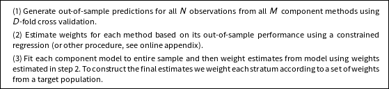
Given the connection between performance in cross validation and accurate estimation of heterogeneous treatment effects, we create our ensemble in three broad steps (van der Laan, Polley, and Hubbard Reference van der Laan, Polley and Hubbard2007). In order to weight methods by their cross validation performance, we first generate outof- sample predictions for each observation using each of the component methods. To do this, we proceed as if we are performing $D$ -fold cross validation: we randomly divide our data into $D$ subsets $(d=1,\ldots ,D)$ .Footnote ³ For each subset $d$ , we train all $M$ component methods using the participants in the other $D-1$ subsets, and often using cross validation within each fold to select tuning parameters. In each step, we set tuning parameters using whatever procedure we will use in the full data set. This might involve additional cross validation steps within each fold. Then, we generate predictions using the trained models and the participants’ in subset $d$ ’s covariates and treatment assignment. The result of this procedure is an $N\times M$ matrix $\widehat{\boldsymbol{Y}}$ where entry $\widehat{Y}_{im}$ contains the outof- sample prediction for participant $i$ from method $m$ .

Second, we estimate the weights using the predictions from the folds of the cross validation. For each participant $i$ we regress the true response, $Y_{i}$ , on the out-of-sample predictions, $(\widehat{Y}_{i1},\widehat{Y}_{i2},\ldots ,\widehat{Y}_{im})$ . Specifically, we fit the model,

(8) $$\begin{eqnarray}\displaystyle Y_{i}=\mathop{\sum }_{i=1}^{M}w_{m}\widehat{Y}_{im}+\unicode[STIX]{x1D716}_{i} & & \displaystyle\end{eqnarray}$$

where $\unicode[STIX]{x1D716}_{i}$ is an error term. To ensure that each $w_{m}$ are weights, we impose two constraints on $\boldsymbol{w}_{m}$ : that the weights sum to $1(\sum _{i=1}^{M}w_{m}=1)$ and that the weights are greater than zero ( $w_{m}\geqslant 0$ ). Fitting this regression is a straightforward quadratic programming problem, whose solution provides a set of weight estimates $\widehat{\boldsymbol{w}}$ that we will use to produce our final ensemble. A method’s weight will depend upon its accuracy in the cross validation folds and the distinctiveness of the predictions (van der Laan, Polley, and Hubbard Reference van der Laan, Polley and Hubbard2007).

In the third and final step we use the weights and the component methods to generate an ensemble. We fit each of the component models to the entire sample, creating a prediction function for each method $m$ , ${\hat{g}}_{m}(\cdot )$ . To create final estimates of interest, we generate synthetic observations (Green and Kern Reference Green and Kern2012), with covariates $\boldsymbol{x}$ and treatments $\boldsymbol{T}$ . For discrete covariates we generate all unique covariate and treatment combinations. For continuous covariates we vary over the range of the covariate. We then use the component methods to generate estimates of the heterogeneous effects for each of the component methods. For each synthetic observation $i$ we obtain ${\hat{g}}_{m}(\boldsymbol{T}_{i},\boldsymbol{x}_{i})$ . We then use the estimated weights to create a weighted average for each observation, $\hat{\unicode[STIX]{x1D719}}(\boldsymbol{T}_{i},\boldsymbol{x}_{i})=\sum _{m=1}^{M}{\hat{w}}_{m}{\hat{g}}_{m}(\boldsymbol{T}_{i},\boldsymbol{x}_{i})$ . Using the per-synthetic unit effects, we can then summarize the effect further, taking averages according to appropriate weights. We summarize the steps of the process in Table 1.

Table 1.

Super learnings’s three steps to generating ensemble estimates for heterogeneous treatment effects.

The weighting procedure ensures that we can include many different kinds of methods, even if those methods have closely related assumptions (van der Laan, Polley, and Hubbard Reference van der Laan, Polley and Hubbard2007). The general advice is to include more methods in the ensemble. Additional, correlated predictions will be downweighted in the weighting step. Distinct methods will ensure that different data generating processes are included in the ensemble. In general, adding more models will improve the performance of the ensemble. Of course, we should not take the position too far. Additional methods may add little new information if correlated with already included methods and might slow down the estimation procedure.Footnote ⁴ If scholars are in a position where they need to limit the number of included methods, we recommend including methods that make different fundamental assumptions about the underlying data generating process, rather than methods that have the same assumed underlying process but different tuning parameters.

4 Monte Carlo Simulations of Ensemble Based Methods

We use a series of Monte Carlo simulations to show the ensemble accurately estimates heterogeneous effects.Footnote ⁶ The strong performance of the ensemble is not surprising, particularly given ensemble methods strong performance at classification and prediction tasks (van der Laan, Polley, and Hubbard Reference van der Laan, Polley and Hubbard2007; Hillard, Purpura and Wilkerson Reference Hillard, Purpura and Wilkerson2008; Raftery et al. Reference Raftery, Gneiting, Balabdaoui and Polakowski2005; Montgomery, Hollenbach, and Ward Reference Montgomery, Hollenbach and Ward2012). Our simulations show that by evaluating methods’ predictive performance, ensembles attach greater weight to methods that provide better estimates of the heterogeneous effects.Footnote ⁷

We assess the performance of the ensemble across four distinct data generating processes, averaging the performance of the ensemble over 5 instances of the data generating process. The simulated data generating processes vary in the number of treatments that have systematic effects, the number of treatments that have heterogeneous effects with the included covariates, and the type of covariates that are included in the simulation. In two simulations, Monte Carlo 1 and Monte Carlo 2 are sparse data generating processes—with many of the simulated treatments specified to have an undetectable systematic effect and only a few specified to have heterogeneous effects. Monte Carlo 3 and Monte Carlo 4, specify data generating processes that are more dense—with more treatments having systematic (and large) effects and heterogeneity across covariates. We provide specific details of each data generation process in the online appendix.

We apply our complete ensemble method to each of the simulated data set. In the Monte Carlo simulations—and in our applications, below—we form an ensemble with nine methods: (1) LASSO (Hastie, Tibshirani and Friedman Reference Hastie, Tibshirani and Friedman2001); (2) Elastic Net, with the mixing parameter set to 0.5 (Hastie, Tibshirani and Friedman Reference Hastie, Tibshirani and Friedman2001); (3) Elastic Net, with the mixing parameter set to 0.25 (Hastie, Tibshirani and Friedman Reference Hastie, Tibshirani and Friedman2001); (4) Find It (Imai and Ratkovic Reference Imai and Ratkovic2013); (5) Bayesian GLM (Gelman et al. Reference Gelman, Jakulin, Pittau and Su2008); (6) Bayesian Additive Regression Trees (BART) (Chipman, George, and McCulloch Reference Chipman, George and McCulloch2010; Green and Kern Reference Green and Kern2012); (7) Random Forest (Breiman Reference Breiman2001; Wager and Athey Reference Wager and Athey2017); (8) KRLS (Hainmueller and Hazlett Reference Hainmueller and Hazlett2013); and a (9) Support Vector Machine (SVM) (Platt Reference Platt, Schoelkopf, Burges and Smola1998; Keerthi et al. Reference Keerthi, Shevade, Bhattacharyya and Murthy2001). In the online appendix we provide details for each method’s estimation. After performing 10-fold cross validation to generate predictions, we use Equation 8 to determine each method’s weights. After estimating the weight we then apply the models to the entire sample and create our ensemble estimate of the treatment effects implied by the data generating process as a weighted average of the estimates from each of the component methods.

In addition to comparing the performance of our ensemble estimator to the component methods, we will compare its performance to a naïve ensemble—where all methods are assumed to contribute equally to the average. We measure the performance of the methods using the root mean square error of the estimated heterogeneous treatment effects (MCATEs), with a smaller root mean square error implying more accurate estimates of the heterogeneous effects.

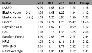
The ensemble method outperforms the other methods across diverse data generating processes in our Monte Carlo simulations. For ease of interpretation, Table 2 presents the performance of each method in terms of the ratio of its root mean squared error to the root mean square error of the ensemble estimate (van der Laan, Polley, and Hubbard Reference van der Laan, Polley and Hubbard2007). If this is greater than 1, then the ensemble has a smaller root mean square error, or performs better in estimating the heterogeneous effects. To calculate the entries in Table 2 we first averaged each method’s performance in five different iterations of the data generating processes and averaged the weighted ensemble’s performance. We then took the ratio of the average mean square errors. In the online appendix we provide the MSE for each iteration of the Monte Carlo simulations.

Table 2.

Across diverse problems, the ensemble estimator performs best (root mean square error of each method relative to root mean square error of the ensemble, reported).

Note: This table shows that the ensemble method outperforms other methods across diverse problems in recovering the heterogeneous treatment effects. This table presents the mean square error for each method averaged over 5 simulations of each data generating process, divided by the mean square error of the ensemble method average over 5 simulations of each data generating process. In individual simulations the ensemble method regularly outperforms the other methods. The right most column shows that, on average, the ensemble estimator has the lowest mean square error across different problems, reflecting its utility as a workhorse tool for estimating MCATEs.

Consider the first two columns in Table 2, showing the results for the sparse data generation processes. Here, we see that methods that assume sparsity perform better—methods such as LASSO. The ensemble outperforms these component methods, however, and is able to more accurately estimate the heterogeneous effects. The third and fourth columns show that methods that assume a dense set of effects and interactions perform better—such as Elastic Net with $\unicode[STIX]{x1D6FC}=0.25$ , KRLS, and Bayesian GLM. Column 5 shows that, as a result, the ensemble estimate has the best average performance across data generating processes and iterations of the simulation. This exemplifies why ensembles are useful: because we never actually know the data generating process, we do not know how well a particular method’s assumptions fit the underlying causal effects (Hastie, Tibshirani and Friedman Reference Hastie, Tibshirani and Friedman2001). Using ensembles ensures that we use methods that reliably capture the heterogeneous effects for a particular problem.

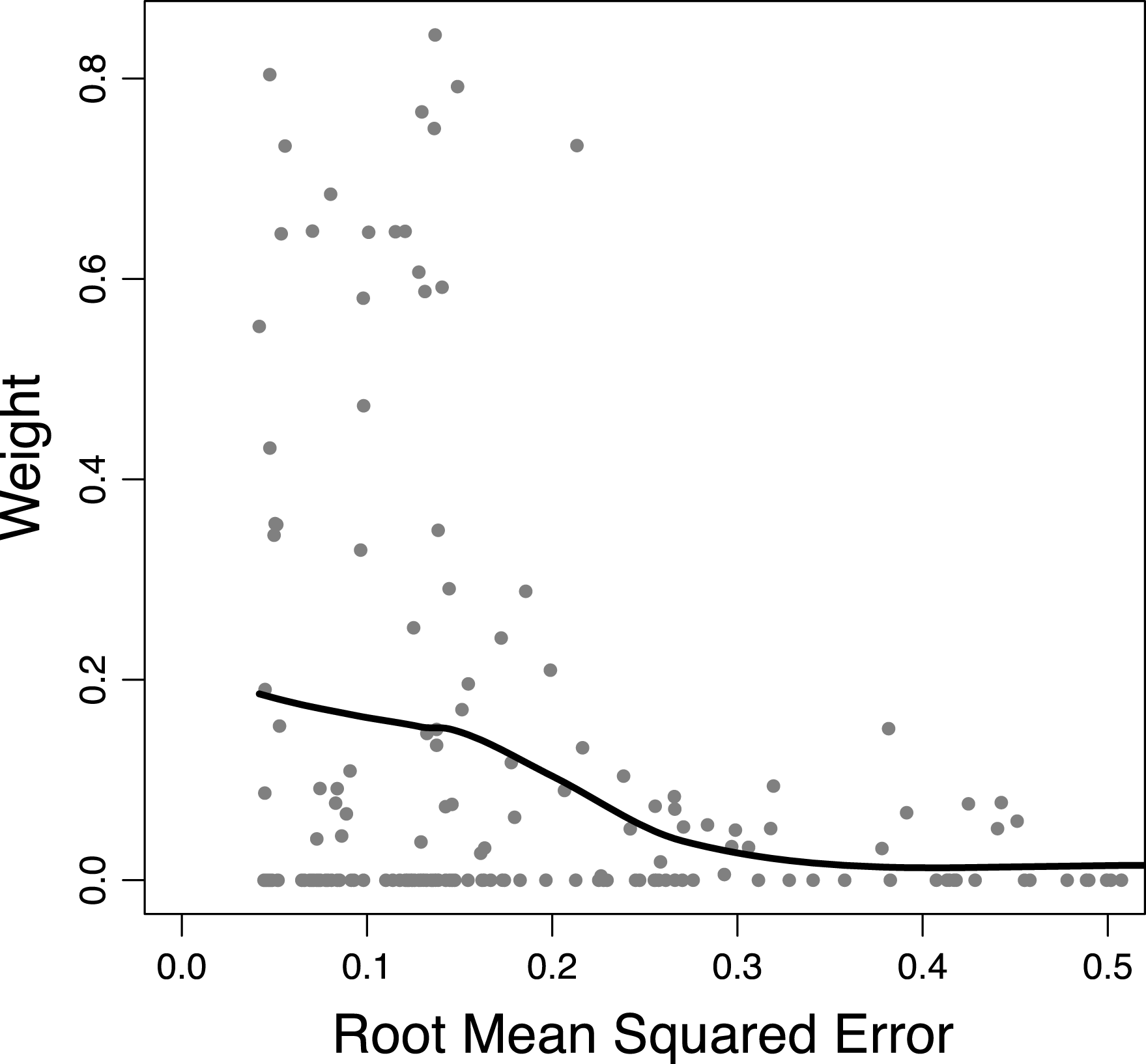
Figure 1 shows why the ensemble is able to outperform the constituent methods: the methods with a smaller RMSE in estimating MCATEs tend to receive more weight in the ensembles (van der Laan, Polley, and Hubbard Reference van der Laan, Polley and Hubbard2007). Figure 1 presents the weight attached to the constituent methods (vertical axis) against the method’s RMSE. This demonstrates a simple relationship: methods with a smaller RMSE in estimating the MCATEs receive greater weight in the final ensemble. Aggregated together, the methods with the best performance receive the greatest weight.Footnote ⁸

Figure 1.

The ensemble tends to place greater weight on methods that more accurately measure heterogeneous treatment effects. (Note: This figure shows that the ensemble method places more weight on methods that more accurately measure the heterogeneous treatment effect. This occurs even though the method is weighting methods that are performing better at out-of-sample prediction. This occurs because of the close connection between estimating heterogeneous treatment effects and predicting outof sample.)

With this strong performance of the methods in mind, we turn now to our applications. We use our methods to reveal how constituents reward legislators for securing money in the district and how constituents punish legislators for budget deficits.

5 Experiment 1: Rewarded For Type of Expenditure, Not Money

Our first experiment reexamines an experiment with heterogeneous treatments and how those treatments vary with respondent characteristics from Grimmer, Westwood, and Messing (Reference Grimmer, Westwood and Messing2014). Grimmer, Westwood, and Messing (Reference Grimmer, Westwood and Messing2014) argue that legislators’ credit claiming statements—a message that legislators use to create the impression they are responsible for some government action—to receive credit for spending in the district and to cultivate a personal vote (Mayhew Reference Mayhew1974; Grimmer, Westwood, and Messing Reference Grimmer, Westwood and Messing2014). The experiment from Grimmer, Westwood, and Messing (Reference Grimmer, Westwood and Messing2014) analyzes how the content of a credit claiming message affects constituent credit allocation. In order to vary many of the features of the experiment, Grimmer, Westwood, and Messing (Reference Grimmer, Westwood and Messing2014) created a template that allows them to vary several features of the message, while maintaining a coherent and realistic message from a legislator. The original authors report marginal effects from the experiment. Our goal in using an ensemble to reanalyze the experiment is to estimate the effects of heterogeneous treatments for exploratory purposes—to identify instances of large scale variation that future experiments could confirm.

Grimmer, Westwood, and Messing (Reference Grimmer, Westwood and Messing2014) assign participants to a control condition (with a 10% chance) or the credit claiming condition (with a 90% chance). Participants in the control condition read a press release from a fictitious representative who “announced that 17-year old Sara Fisher won 1st place in the annual Congressional art competition.” This press release is an example of a common advertising press release—a message devoid of policy content intended to increase the legislators’ prominence (Mayhew Reference Mayhew1974; Grimmer Reference Grimmer2013). The full text of the condition is in Table 3.

Table 3.

Examining the effects of credit claiming statements on constituent credit allocation.

Participants assigned to the credit claiming condition read a message about an expenditure in the district and the fictitious legislator’s role in securing that legislation. To assess how different facets of the credit claiming process affect credit allocation, Grimmer, Westwood, and Messing (Reference Grimmer, Westwood and Messing2014) vary five different components of the message: (1) type of expenditure, (2) amount of money, (3) stage in appropriations process, (4) collaboration with other legislators, and (5) representative’s political party. Varying the features of message simultaneously allow us to identify the kind of information constituents use when evaluating credit claiming messages, in a way analogous to recent conjoint experiments (Hainmueller and Hopkins Reference Hainmueller and Hopkins2015; Hainmueller, Hopkins, and Yamamoto Reference Hainmueller, Hopkins and Yamamoto2014). Table 3 summarizes the conditions and how the information was provided to participants in the study. In addition to the heterogeneous treatments, we also examine how the effects vary across two relevant respondent characteristics: respondent’s partisan identification—respondents classify themselves as a Democrat, Republican, or Independent/Other—and ideological orientation—respondents classify themselves as Conservative, Liberal, or Moderate.

We examine the effect of legislators’ credit claiming efforts on constituents’ propensity to Approve of the representative’s performance in office. Specifically, Grimmer, Westwood, and Messing (Reference Grimmer, Westwood and Messing2014) asked participants if they “approve or disapprove” of the way the fictitious representative “is performing (his/her) job in Congress.” Grimmer, Westwood, and Messing (Reference Grimmer, Westwood and Messing2014) recruited $1,074$ participants on Amazon.com’s Mechanical Turk service, selecting only workers from the United States.Footnote ⁹ After respondents were assigned to a treatment, they completed a brief postsurvey that included questions about the legislator and the respondent’s own personal political preferences.

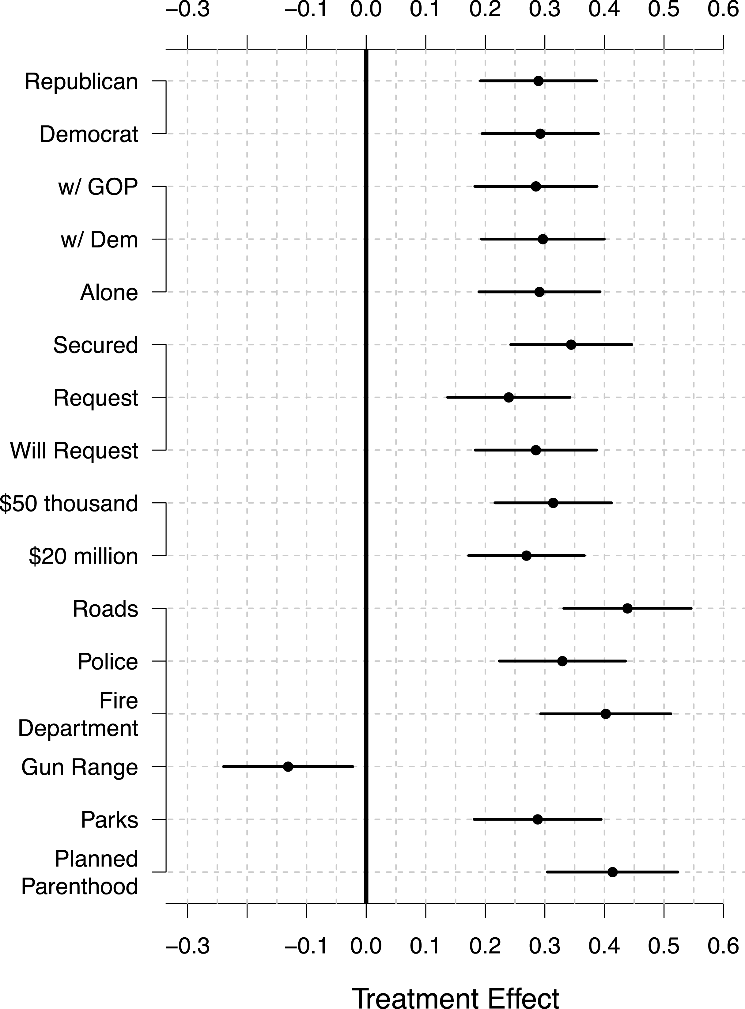
Figure 2 shows the (MATEs), averaging over the accompanying conditions and using the control condition for comparison. The vertical axis shows the information varied in the experiments—including the different types of expenditures, amount of spending, stage in the appropriations process, who announced the expenditure, and the fictitious legislator’s party. The point is the MATE of that condition and the lines are 95 percent confidence intervals.

Figure 2.

The marginal effects of the credit claiming experiment. (Note: This figure shows the marginal effects from the credit claiming experiment. Respondents appear to be evaluating the credit claiming statement based on the type of message, but struggle to include other types of information.)

Figure 2 suggests that participants are able to make use of easily available information—such as the type of expenditure—but struggle to include other types of information in their evaluation of credit allocation. The type of expenditure matters considerably—gun ranges decrease approval for representatives (13.1 percentage point decrease, 95 percent confidence interval [ $-$ 0.25, $-$ 0.01]), but other types of projects legislator increase approval over the control condition (37 percentage point increase, 95 percent confidence interval [0.29, 0.46]). Other information, however, has a smaller effect on constituent credit allocation. There is essentially no difference in the credit awarded legislators if they claim credit for or , who legislators announce with, or whether the legislator is a Democrat or Republican. Securing money does cause an increase in support, relative to stating that the legislator will request or requested the money, with securing causing an 8.1 percentage point great increase in support than requesting or stating an intent to request (95 percent confidence interval [0.02, 0.15]).

The effects in Figure 2 suggest that participants are evaluating legislators’ credit claiming efforts by evaluating the type of expenditure, while struggling to use other information. If true, then how participants evaluate the type of expenditure will depend on their partisanship and ideology. This is clearest for two of the more polarizing types of expenditures Grimmer, Westwood, and Messing (Reference Grimmer, Westwood and Messing2014) included: a gun range and funding for planned parenthood. Liberal elites and Democrats tend to vigorously defend planned parenthood, providing cues to like minded citizens that the organization provides valuable services. In contrast, conservatives and Republicans oppose planned parenthood, often working to strip the organization of money (for example, (Kasperowicz Reference Kasperowicz2013)). Very different cues are available about gun ranges. Many Democrats—particularly liberal-urban Democrats—have argued for increased gun regulation. Republicans and conservatives have argued vigorously for constitutional protection of guns.

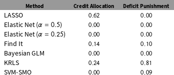
To examine how the message content affects credit allocation across participants with different partisan identifications and ideological orientation we use our ensemble method.Footnote ¹⁰ We apply the ensemble method using $10$ -fold cross validation, then use Equation 8 to estimate the weights attached to each method. The first column of Table 4 shows the weights attached to each method for the ensemble used to generate the effects for this experiment. Three methods receive nonzero weight: LASSO (0.62), KRLS (0.24), and Find It (0.14). In generating the final effects, we compare all treatment effects to the control advertising condition.

Figure 3.

Constituent partisanship and ideology predicts differences in the effectiveness of credit allocation. (Note: This figure shows substantial heterogeneity in how participants respond to the different types of money legislators claim credit for securing.)

Table 4.

The weight attached to methods varies across experiments.

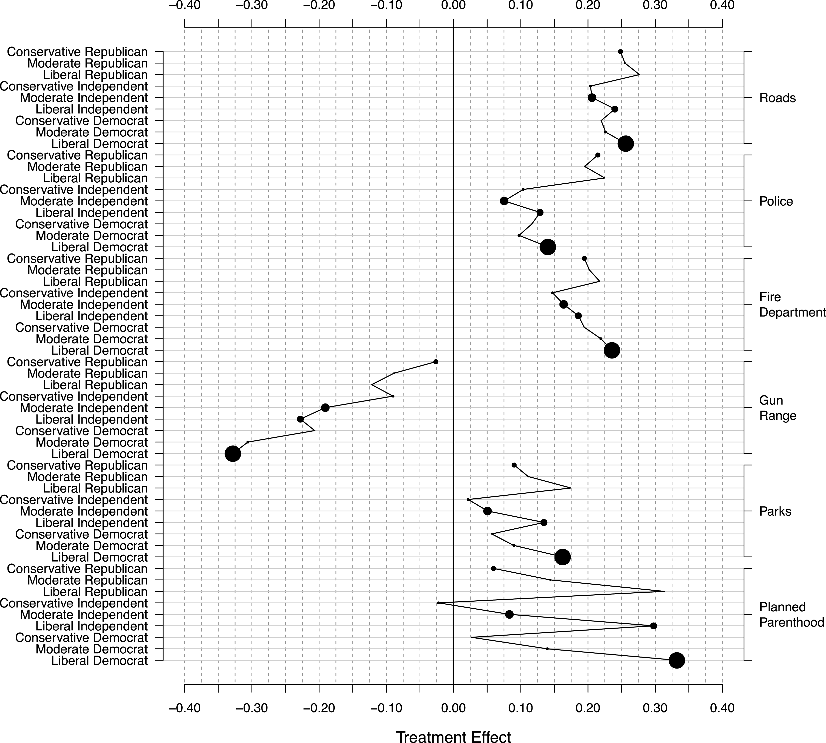
Figure 3 shows how the effect of the type of project claimed depends on the participant’s partisan and ideological identification. On the right-hand side vertical axis we vary the type of expenditure announced and within each type of expenditure we vary participants ideological orientation and partisan identification. To ease interpretation and facilitate exploration, we draw lines to connect the heterogeneous responses to the same type of expenditure.

Figure 3 reveals substantial heterogeneity in the effect of the type of project on constituent credit allocation, consistent with constituents evaluating the type of expenditure when evaluating legislators’ credit claiming statements. Consider the response to money directed to planned parenthood. Liberal respondents, regardless of partisan affiliation, boost support for the representative who claims credit for securing money for planned parenthood. The fictitious legislator claiming credit for funds for planned parenthood caused a 30 percentage point increase in approval rating for liberals. Conservatives, however, have a more muted—and even negative—response to legislators who claim credit for planned parenthood spending. Indeed, claiming credit for money delivered to planned parenthood causes a decrease in approval ratings among independent conservatives and only a small increase among other conservatives. Of course, our visualization shows that there are few conservatives in our MTurk sample, leading us to have some caution in interpreting the findings for conservatives.

The effect of claiming credit for gun ranges also varies across participants. Constituents who are likely to have a negative attitude about guns have a strong negative reaction to legislators claiming credit for a new gun range. Claiming credit for a gun range causes an over 30 percentage point decline in a legislators’ approval rating among liberal Democrats. But constituents who are likely to have a less negative view of guns have a more muted response to the gun range: claiming credit for a gun range causes only a 5 percentage point decline among conservative Republicans. But again, note the small sample of conservative Republicans in our MTurk sample. Conservatives and Republicans do not, however, simply have a smaller magnitude to all credit claiming efforts. Claiming credit for delivering money to police causes a 21 percentage point increase in approval among Republicans, while only an 11 percentage point increase among Democrats and independents.

Figure 4.

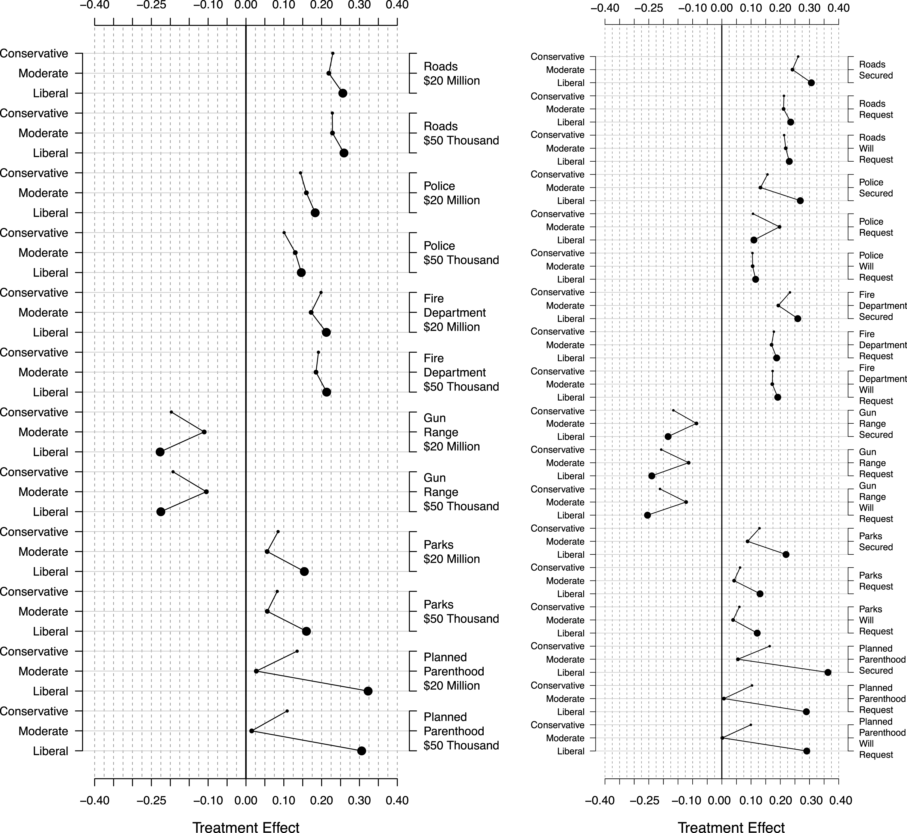
The money secured or the stage in the process appears to be less important. (Note: This figure shows that constituents struggle to include information about the amount of money legislators claim credit for securing (left-hand plot) or the stage in the process that the money is in (right-hand plot).)

The heterogeneity in response to the type of credit claiming message is consistent with constituents evaluating the type of expenditure when allocating credit for spending in the district. Figure 4 shows that constituents tend to be less responsive to other pieces of information in the credit claiming statements. The left-hand plot in Figure 4 shows how the effect of the type of project and the amount of money (right-hand vertical axis) for the project varies across constituent ideology. This figure shows that constituents—across types of expenditure and ideological orientation—are largely unaffected by the amount claimed. Indeed the parallel lines are indicative of constituents who are largely unable to incorporate information about the size of the expenditure into their overall evaluations. Consistent with evidence from Grimmer, Messing, and Westwood (Reference Grimmer, Messing and Westwood2012), the size of the expenditure appears to matter little when constituents are allocating credit to legislators. The right-hand plot in Figure 4 shows how the effect of credit claiming messages varies across type of money secured and stage in the appropriations process (right-hand vertical axis) and constituents’ ideological orientation (left-hand vertical axis). While there is evidence that constituents do reward the fictitious legislator slightly more for securing rather than requesting money, the increase from having secured an expenditure appears to be much smaller than the heterogeneity across the type of expenditure.

This section uses the ensemble method for estimating heterogeneous treatment effects to explore the types of information constituents use when responding to legislators’ credit claiming messages. This shows that constituents tend to evaluate easily available information—such as the type of money secured—but struggle to include information about the amount that legislators secured. Together, this shows how the ensemble of heterogeneous treatment effect methods can be used as an exploratory tool—to identify how the components of the messages vary across respondents. To validate this exploration, additional experiments could be run that explicitly test the heterogeneity discovered here along with a pre-analysis plan, ensuring that our exploration is not biasing the inferences we make (Humphreys, Sanchez de la Sierra, and van der Windt Reference Humphreys, de la Sierra and van der Windt2013).

5.1 Experiment 2: Punishment for budget deficits

Several studies argue that legislators claim credit for spending to cultivate a personal vote with constituents. Yet, in recent years a growing movement of conservatives, the Tea Party, has criticized expenditures as wasteful (Skocpol and Williamson Reference Skocpol and Williamson2011). Grimmer, Westwood, and Messing (Reference Grimmer, Westwood and Messing2014) design an experiment to assess how the criticism of government spending affects how constituents allocate credit. Grimmer, Westwood, and Messing (Reference Grimmer, Westwood and Messing2014) show that labeling an expenditure as contributing to the budget deficit undermines the credit legislators’ receive. We apply the ensemble method to assess how the effect of the criticism varies across constituent characteristics—revealing that the effect of budget criticism varies substantially, depending on constituents’ ideological orientation. While the previous example shows how the method can be used to estimate the effect of heterogeneous treatment, this example focuses on how the method can be used to estimate the heterogeneous effect of a relatively simple intervention.

Grimmer, Westwood, and Messing’s (Reference Grimmer, Westwood and Messing2014) experiment couples a legislator’s claiming credit for an expenditure with criticism about the budget implications of the spending. For realism about the magnitude of the effects, this experiment utilizes participants’ actual representatives, rather than fictitious representatives used in the first study. Table 5 contains the content of the experiment’s three conditions. In the credit claiming condition participants are presented with their house member claiming credit for an highway expenditure in their Congressional district. To customize the paragraph about each participant’s legislator, Grimmer, Westwood, and Messing (Reference Grimmer, Westwood and Messing2014) insert the representative’s name at $|$ representativeName and the participant’s state at $|$ state in the text.

Two budget criticism conditions vary the source of the information about how the spending will affect the federal deficit. The CBO Budget Information condition includes this same credit claiming about a highway expenditure, but pairs it with information about the budget consequences of the expenditure from the nonpartisan Congressional Budget Office (CBO). This condition has an official statement from the CBO, which includes the overall cost of the program and that expenditure would be deficit spending. In the Partisan Information condition, participants receive budget information from a political figure likely to criticize the participant’s member of Congress: the opposing party’s national chairperson. Participants with a Democratic representative see a statement from Reince Priebus—chair of the Republican national committee—and participants with a Republican member of Congress see a statement from Debbie Wasserman-Schultz—chair of the Democratic national committee.

Table 5.

Content across conditions, experiment 2.

Grimmer, Westwood, and Messing (Reference Grimmer, Westwood and Messing2014) administered the experiment to 1,166 participants, using a census matched US sample from a Survey Sampling International (SSI) panel. Participants were assigned to conditions, the treatments were administered, and then a postsurvey was administered. Grimmer, Westwood, and Messing (Reference Grimmer, Westwood and Messing2014) shows that the budget criticism have a strong and negative effect on legislators’ approval ratings. The budget information from the CBO causes an overall decrease of 8.2 percentage points (95 percent confidence interval [-0.16, -0.01]) and the partisan information causes a similar overall decrease in approval of 7.7 percentage points (95 percent confidence interval [-0.15, -0.00]).

To examine how the effects of the intervention vary across constituent and legislator characteristics, we apply the ensemble method to the experiment. Table 4 shows the diverse methods that receive weight for this experiment: including KRLS (0.81), Find It (0.10), and SVM (0.09). We then use the ensemble to compute MCATEs for combinations of respondent characteristics and particular treatments, with all effect sizes based on a comparison to the credit claiming message without criticism.

Table 6.

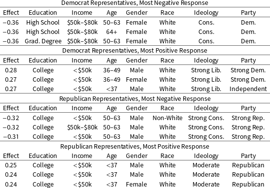
Characteristics of constituents with the most negative response to budget criticism for democrat and republican representatives.

Following Imai and Strauss (Reference Imai and Strauss2011) and Imai and Ratkovic (Reference Imai and Ratkovic2013), we first use the ensemble method to assess the constituents who have the most negative and positive response to the criticism. Table 6 shows who has the most negative and positive response to the budget criticisms for Democratic and Republican representatives. The most negative responses for both Democratic and Republican representatives come from constituents who identify as conservative—strong conservatives for Republican representatives, conservatives for Democratic representatives. For Democratic legislators the most positive response comes from strong liberals who are also strong Democrats—the most positive response for Republican representatives is from moderate Republicans.

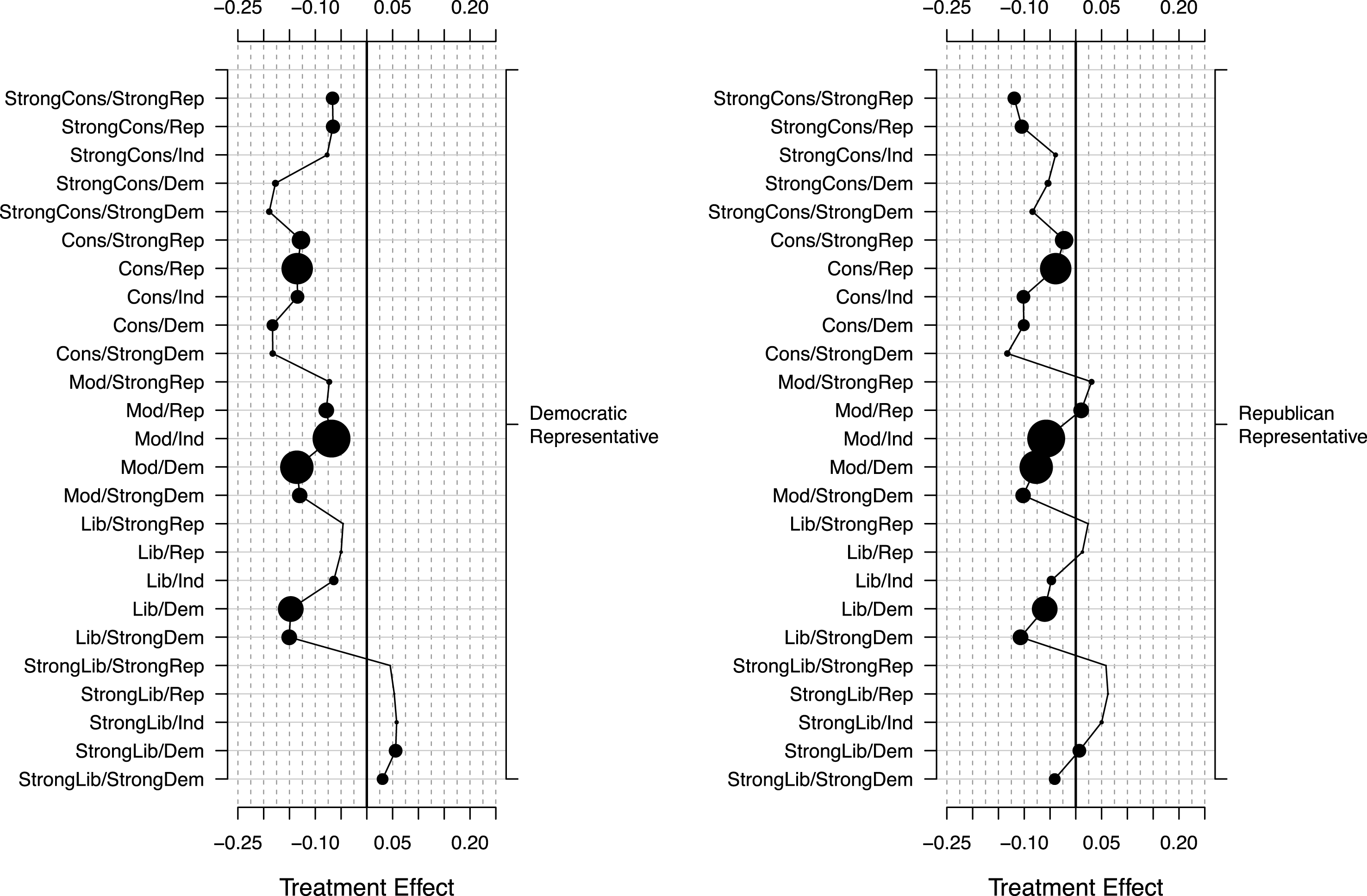
Table 6 reveals who has the strongest response to the budget criticism treatment, suggesting that conservatives are particularly likely to punish legislators for deficit spending and that strong liberals are particularly likely to reject the criticism. To examine how the effect of the criticism varies across different types of respondents, Figure 5 shows how the effect of the budget criticism affects credit allocation for Democratic (left-hand plot) and Republican representatives (right-hand plot) and for constituents with varying ideological orientations (strong liberal, liberal, moderate, conservative, strong conservative) and partisan affiliations (strong Democrat, Democrat, Independent, Republican, strong Republican). This figure shows that strong liberals—particularly strong liberals with a Democratic representative—tend to have a positive response to the budget criticism. This aligns well with cues from political elites, who have suggested that deficit spending does less harm than members of the political right emphasize. Further, moderate Republicans appear unaffected by information about spending’s budget implications. Conservatives, however, have a particularly negative response to learning about the budget implications of an expenditure. And as Table 6 illuminates, strong conservatives have a particularly negative response to the criticism.

Figure 5.

Strong liberals are unresponsive to budget criticisms. (Note: This figure shows how the response to budget criticism depends on constituents’ characteristics (left-hand vertical axis). For both Democrats and Republicans (right-hand vertical axis), we see that Strong liberals are unresponsive to the budget criticism, or the criticism may cause an increase in legislators’ approval ratings. Strong conservatives, however, a much more negative reaction to the credit claiming efforts. This is consistent with the rise of the Tea Party movement.)

The variation in response to the budget criticism aligns with intuition about how Tea Party rhetoric affects how constituents respond to budget criticism. For participants likely to be receptive to the rhetoric—conservatives—the budget criticism causes sharp punishment of the elected official. But for other constituents, the budget criticism is ineffective. Strong liberals—who have likely learned of the arguments for deficit spending—are unperturbed by the criticism and continue allocating credit to legislators for spending—in some cases greater expenditures. Together, the heterogeneity in response illuminates how critical rhetoric can make it costly for Republicans to claim credit for spending, because they depend on the support of strong conservatives in the primary. Democrats, however, do not have the same costs, because the most ideological members of their base—strong liberals, have a positive response to the budget criticism.