
1. Introduction
This paper aims to find a priori complex growth rate bounds of ideal wave-like perturbations on top of compressible, stratified, magnetised and sheared equilibrium states varying in two directions perpendicular to the direction of the wave propagation.
Growth rate bounds and stability criteria of ideal shear flows have long been some of the central issues in theoretical fluid mechanics. Rayleigh's inflection point theorem (Rayleigh Reference Rayleigh1880), Howard's semicircle theorem (Howard Reference Howard1961) and the Miles–Howard stability condition (Miles Reference Miles1961) are particularly well known across the fluid dynamics, geophysics and astrophysics communities, and their various extensions have been sought. One obvious way of extending the theories is to make the base-state variation two-directional as in many practical problems. However, far less progress has been made for the theoretical understanding of such generalised stability problems compared with the classical cases, in particular when there are multiple physical effects such as compressibility, stratification and magnetohydrodynamic effects. The major difference between the planar and non-planar cases is that for the former classical cases, the motion of the perturbation might be restricted on a two-dimensional plane. In the geophysics community, the stability theory has been advanced using the fact that multiple Casimir invariants are available for two-dimensional fluid motion when it is viewed in the Hamiltonian mechanics framework (see Arnold Reference Arnold1978; Dowling Reference Dowling1995, for example). While for the generalised problem the perturbation is inherently three-dimensional, and so fewer mathematical tools are available. Whether the classical planar results can be carried over to non-planar cases is, in general, a non-trivial question.
The non-planar magnetohydrodynamic stability problems may have some relevance to cutting-edge industrial applications such as fusion reactors or magnetohydrodynamic electric generators. For example, the magnetohydrodynamic flows through ducts of complicated cross-sections commonly appear in some fusion blanket designs. The Hunt flow in a rectangular duct may be one of the simplest models for this problem, where the inviscid instability indeed plays important roles (Priede, Aleksandrova & Molokov Reference Priede, Aleksandrova and Molokov2010; Qi et al. Reference Qi, Liu, Ni and Yang2017). Even in such a simple case, the stability computation is not easy, especially in the high-Reynolds-number range. Moreover, when the duct has sharp corners, the singularities there affect the numerical eigenvalues badly. If fins of complex shape are attached to enhance heat transfer, the computation becomes practically impossible.
The flow fields to be treated in this paper may also have important implications for solar physics. For example, just underneath the Sun's surface, there is a shear layer called tachocline (see the paper by Charbonneau et al. (Reference Charbonneau, Tomczyk, Schou and Thompson1998), for example) and the stability of it has been a subject of many astrophysics studies, wherein the planar version of our base flow is commonly used. In the early years of the stability analyses in solar physics, the effect of shear was omitted because, in that case, the stability can be analysed by simply examining the property of the Lagrangian potential energy (Bernstein et al. Reference Bernstein, Frieman, Kruskal and Kulsrud1958; Newcomb Reference Newcomb1961; Parker Reference Parker1966). Frieman & Rotenberg (Reference Frieman and Rotenberg1960) introduced the effect of shear to the energy principle theory, and based on the extended principle, Adam (Reference Adam1978a) and Tobias & Hughes (Reference Tobias and Hughes2004) subsequently developed some stability conditions; we will add further comments on those studies later.
Here, we summarise the previous (mostly planar) stability results that are relevant to our results. The semicircle theorem by Adam (Reference Adam1978b) is particularly relevant to the present study because it is shown for the two-dimensional version of the magnetoatmospheric flow configuration to be considered in this paper. In the first half of this paper, we will extend the application range of his result significantly and, in addition, improve the eigenvalue bound itself. Hughes & Tobias (Reference Hughes and Tobias2001) found that there are two semicircles possible, and union of them will give a net bound. Motivated by this result, we shall show that actually, infinitely many semicircle bounds can be defined, and the union of them constitutes the eigenvalue bound better than that of the usual semicircle. Another improvement shown by Hughes & Tobias (Reference Hughes and Tobias2001) is that the semicircle radius can be contracted when the external magnetic field presents. The same result was shown by Cally (Reference Cally2000), who found that the contraction discovered by Howard & Gupta (Reference Howard and Gupta1962) and Gupta (Reference Gupta1992) for a uniform magnetic field case can be carried over to inhomogeneous magnetic fields. The stabilisation effect of the magnetic field may also be seen for compressible flows, in view of the stability condition found by Cally (Reference Cally2000). This is in fact true, as we shall show in this paper, although there is a condition for the stabilisation to occur.
In the latter half of this paper, we shall derive two other types of bounds using the Miles–Howard theory. The theory differs fundamentally from the semicircle-type theories, in that the stability condition deduced by it depends on the velocity shear rather than the velocity range. Our second bound is similar to the semi-ellipse bound of Kochar & Jain (Reference Kochar and Jain1979), who found that the inequality derived from the Miles–Howard theory can be used to improve the semicircle eigenvalue bound. Fung (Reference Fung1986) attempted to extend the semi-ellipse theorem to flows subjected to a general conservative force field varying in two directions. However, Fung (Reference Fung1986) implicitly assumed a condition that can only be satisfied for quite specific flows. Our bound is found by considering the correct extension of the semi-ellipse theorem, even including the compressibility and magnetohydrodynamic effects, which were not considered by Kochar & Jain (Reference Kochar and Jain1979) and Fung (Reference Fung1986). The third bound to be found in this paper is the non-planar version of the bound found by Cally (Reference Cally1983), which also depends on the velocity shear. As Cally's derivation cannot be extended to the generalised flows, we instead use the Miles–Howard theory in the proof.
Among all the above previous stability results, the incompressible result by Gupta (Reference Gupta1992) is the only work where a magnetised problem was treated in the base shear with variation of the flow in two directions. For non-magnetised flows, to the best of the author's knowledge, Eckart (Reference Eckart1963) and Hocking (Reference Hocking1964) were the first to consider such an extension, with the former showing that Howard's semicircle theorem holds for some cases and the latter leading to limited results for special flow fields. The work by Eckart (Reference Eckart1963) seems to be often cited in the context of adding compressibility to the semicircle theorem, and the aspect of dealing with a flow that varies in two directions is less well known. Perhaps for this reason, many authors subsequently reported semicircle theorems that are covered by Eckart's result (e.g. the papers by Blumen (Reference Blumen1975) for convectively stably stratified Boussinesq flows, by Dandapat & Gupta (Reference Dandapat and Gupta1977) for compressible, unstratified flows, and by Li (Reference Li2011) and Waleffe (Reference Waleffe2019) for incompressible, unstratified flows).
Numerical stability analyses of inviscid flows varying in two directions are in general very challenging, unlike the classical planar versions for which we can use the shooting method. For the simplest case where the flow is incompressible, non-magnetised and unstratified, Hall & Horseman (Reference Hall and Horseman1991), Yu & Liu (Reference Yu and Liu1991), Li & Malik (Reference Li and Malik1995) and Andersson et al. (Reference Andersson, Brandt, Bottaro and Henningson2001) successfully computed the stability of the streak (which of course varies in two directions, because it refers to heterogeneity in the velocity field created by weak vortices elongated in the flow direction). However, for flows with more complex physical effects, such as those considered in this paper, no numerical results have been reported. The significance of this paper is that we have developed a quick and simple method to study such challenging eigenvalue problems. The bounds to be derived can be easily calculated for quite a wide range of flow configurations to observe the overall character of the eigenvalues. A particularly important practical engineering application would be the stability problem of the aforementioned magnetohydrodynamic flows through ducts with a complex cross-section.
Although ideal stability analyses might seem somewhat classical, the importance of it in turbulence is increasingly recognised in the fluid dynamics community. There is much evidence that the instability waves on top of the streak indeed play crucial roles in fully developed near-wall turbulent flows (Hamilton, Kim & Waleffe Reference Hamilton, Kim and Waleffe1995; Jimenez & Pinelli Reference Jimenez and Pinelli1999; McKeon & Sharma Reference McKeon and Sharma2010; Thomas et al. Reference Thomas, Lieu, Jovanovic, Farrell, Ioannou and Gayme2014; Alizard Reference Alizard2015; Beaume et al. Reference Beaume, Chini, Julien and Knobloch2015). If we accept this view, the complex eigenvalue bounds should have an important implication for the properties of turbulent bursts. Furthermore, when the amplitude of the instability waves of the streak reaches a certain magnitude, they eventually drive the streak field via Reynolds stress (see Benney Reference Benney1984; Hall & Smith Reference Hall and Smith1991; Waleffe Reference Waleffe1997). The resultant nonlinear loop between the streak and the waves constitutes the basis of the self-sustainment mechanism of coherent structures in near-wall turbulence and has recently attracted much attention. Interestingly, at high Reynolds numbers, the mechanism by which the instability wave of the streak is generated can be well described by the inviscid theory. Indeed, the fact that the generalised ideal stability problem sits at the centre of the sustainment process has inspired the recent two re-discoveries of the semicircle theorem (Li Reference Li2011; Waleffe Reference Waleffe2019).
The paper is organised as follows. Section 2 formulates the problem based on the ideal compressible magnetohydrodynamic equations under the influence of the general conservative force field. We will show that the linear stability problem can be reduced to three equations for the Lagrangian displacement vector, or alternatively, a single equation for the total pressure perturbation. In § 3, we will first describe the derivation of the semicircle bound based on the energy principle theory, and then see how the bound can be improved by more effectively using the property of the potential energy. The primary focus of § 4 is to clarify when the Miles–Howard theory can be used for the generalised non-planar flows. The results obtained in the generalised theory will then be used to develop a semi-ellipse-type bound and a Cally-type bound, both of which are generalised for non-planar flows. The three bounds are compared with numerical eigenvalues in § 5. Finally, in § 6, we will draw some conclusions.
2. Formulation of the problem
2.1. Derivation of the stability problem
Consider the ideal compressible magnetohydrodynamic equations in Cartesian coordinates  $(x,y,z)$.
 \begin{gather} \rho(\partial_{t}+\boldsymbol{v}\boldsymbol{\cdot} \boldsymbol{\nabla})\boldsymbol{v} ={-}\boldsymbol{\nabla} q+\frac{1}{\mu_0}(\boldsymbol{b}\boldsymbol{\cdot} \boldsymbol{\nabla})\boldsymbol{b}+\rho \boldsymbol{\nabla} G, \end{gather}
 \begin{gather}\partial_{t}\boldsymbol{b} = \boldsymbol{\nabla} \times (\boldsymbol{v}\times \boldsymbol{b}), \end{gather}
 \begin{gather}\partial_{t} \rho+ \boldsymbol{\nabla} \boldsymbol{\cdot} (\rho \boldsymbol{v})=0, \end{gather}
 \begin{gather}(\partial_{t}+\boldsymbol{v}\boldsymbol{\cdot} \boldsymbol{\nabla})(\rho^{-\gamma} p)=0. \end{gather}
The first equation is the momentum conservation equation, the second equation is the induction equation, the third equation is the mass conservation equation and the fourth equation is the adiabatic energy conservation equation. In addition, we assume that Gauss's law  $\boldsymbol {\nabla } \boldsymbol {\cdot } \boldsymbol {b}=0$ holds. Throughout the paper, we denote the velocity vector as
 $\boldsymbol {v}=(v^x,v^y,v^z)$, the magnetic field vector as
 $\boldsymbol {b}=(b^x,b^y,b^z)$, the density as
 $\rho$, the kinematic pressure as
 $p$ and the total (i.e. kinematic and magnetic) pressure as
 $q=p+|\boldsymbol {b}|^2/2\mu _0$. The momentum equations are subjected to a conservative field with potential
 $G(y,z)$, as in the paper by Fung (Reference Fung1986). The adiabatic exponent
 $\gamma$ and the vacuum permeability
 $\mu _0$ are constants.
Our interest is the stability of a quasi-equilibrium base state depending on  $y,z$. The base velocity
 $\boldsymbol {v}=(\bar {u}(y,z),0,0)$ and magnetic field
 $\boldsymbol {b}=(\bar {B}(y,z),0,0)$ are assumed to be unidirectional. Those fields may be driven by some external forcing applied on the streamwise component of the momentum and induction equations, or may be developing on a slower time scale than that of the ideal instability. From the
 $y,z$ components of the momentum equations, it is easy to see that the base total pressure
 $\bar {q}(y,z)$ and the base density
 $\bar {\rho }(y,z)$ must satisfy the magnetostatic conditions:
 \begin{equation} \bar{q}_y-\bar{\rho}G_y=\bar{q}_z-\bar{\rho}G_z=0,\end{equation}
which imply
 \begin{equation} \frac{G_y}{\bar{\rho}_y}=\frac{G_z}{\bar{\rho}_z}.\end{equation}
Here and hereafter, the subscripts  $y$ and
 $z$ represent corresponding partial differentiation.
The stability of the base flow can be found by adding an infinitesimally small normal mode perturbation:
 \begin{gather} \boldsymbol{v}= \left[ \begin{array}{@{}c@{}} \bar{u}(y,z)\\0\\0 \end{array} \right] + \left[ \begin{array}{@{}c@{}} \tilde{v}^x(y,z)\\ \tilde{v}^y(y,z)\\ \tilde{v}^z(y,z) \end{array} \right]\textrm{e}^{\textrm{i}k (x-ct)}+\text{c.c.}, \end{gather}
 \begin{gather}\boldsymbol{b}= \left[ \begin{array}{@{}c@{}} \bar{B}(y,z)\\0\\0 \end{array} \right] + \left[ \begin{array}{@{}c@{}} \tilde{b}^x(y,z)\\ \tilde{b}^y(y,z)\\ \tilde{b}^z(y,z) \end{array} \right]\textrm{e}^{\textrm{i}k(x-ct)}+\text{c.c.}, \end{gather}
 \begin{gather}\rho=\bar{\rho}(y,z)+\tilde{\rho}(y,z)\,\textrm{e}^{\textrm{i}k (x-ct)}+\text{c.c.}, \end{gather}
 \begin{gather}p=\bar{p}(y,z)+\tilde{p}(y,z)\,\textrm{e}^{\textrm{i}k (x-ct)}+\text{c.c.}, \end{gather}
 \begin{gather}q=\bar{q}(y,z)+\tilde{q}(y,z)\,\textrm{e}^{\textrm{i}k (x-ct)}+\text{c.c.}, \end{gather}
where the Fourier transformed perturbation quantities  $\tilde {v}^x,\tilde {v}^y,\tilde {v}^z,\tilde {b}^x,\tilde {b}^y,\tilde {b}^z,\tilde {\rho },\tilde {p},\tilde {q}$ are complex functions and c.c. stands for complex conjugate. Here,
 $k>0$ is the streamwise wavenumber and
 $c=c_r+ic_i$ is the complex wave speed. We remark here that from the definition of the total pressure, the base and perturbation kinetic pressures should satisfy
 $\bar {p}=\bar {q}-\bar {B}^2/2\mu _0$ and
 $\tilde {p}=\tilde {q}-\bar {B}\tilde {b}^x/\mu _0$, respectively.
Substituting (2.4) to (2.1) and neglecting all the nonlinear terms, we find
 \begin{align} &\bar{\rho} \left\{ Uik \left[ \begin{array}{c} \tilde{v}^x\\ \tilde{v}^y\\ \tilde{v}^z \end{array} \right] + \left[ \begin{array}{c} \tilde{v}^yU_y+\tilde{v}^zU_z\\ 0\\ 0 \end{array} \right] \right\} \nonumber\\ &\quad -\frac{1}{\mu_0}\left\{ \bar{B}ik \left[ \begin{array}{c} \tilde{b}^x\\ \tilde{b}^y\\ \tilde{b}^z \end{array} \right] + \left[ \begin{array}{c} \tilde{b}^y\bar{B}_y+\tilde{b}^z\bar{B}_z\\ 0\\ 0 \end{array} \right] \right\} +\left[ \begin{array}{c} ik \tilde{q} \\ \tilde{q}_y-G_y\tilde{\rho} \\ \tilde{q}_z-G_z\tilde{\rho} \end{array} \right]=0, \end{align}
 \begin{align} &\left\{ Uik \left[ \begin{array}{c} \tilde{b}^x\\ \tilde{b}^y\\ \tilde{b}^z \end{array} \right] + \left[ \begin{array}{c} \tilde{v}^y\bar{B}_y+\tilde{v}^z\bar{B}_z\\ 0\\ 0 \end{array} \right] \right\} \nonumber\\ &\quad - \left\{ \bar{B}ik \left[ \begin{array}{c} \tilde{v}^x\\ \tilde{v}^y\\ \tilde{v}^z \end{array} \right] + \left[ \begin{array}{c} \tilde{b}^yU_y+\tilde{b}^zU_z\\ 0\\ 0 \end{array} \right] \right\} + \left[ \begin{array}{c} \bar{B}(ik \tilde{v}^x+\tilde{v}_y^y+\tilde{v}_z^z)\\ 0\\ 0 \end{array} \right] =0, \end{align}
 \begin{gather} ik \tilde{b}^x+\tilde{b}_y^y+\tilde{b}_z^z=0, \end{gather}
 \begin{gather}U ik \tilde{\rho}+(\tilde{v}^y\bar{\rho}_y+\tilde{v}^z\bar{\rho}_z)+\bar{\rho}(ik \tilde{v}^x+\tilde{v}_y^y+\tilde{v}_z^z)=0, \end{gather}
 \begin{gather}U ik \left(s^2 \tilde{\rho}+\frac{\bar{B}\tilde{b}^x}{\mu_0}-\tilde{q}\right)+ \tilde{v}^y\left(s^2 \bar{\rho}_y+\frac{\bar{B}\, \bar{B}_y}{\mu_0}-G_y\bar{\rho}\right)+ \tilde{v}^z\left(s^2 \bar{\rho}_z+\frac{\bar{B}\, \bar{B}_z}{\mu_0}-G_z\bar{\rho}\right)=0. \end{gather}
Here the local sound wave speed  $s$ and the shifted base velocity
 $U$ have been defined as
 \begin{equation} s(y,z)\equiv \sqrt{\frac{\gamma\bar{p}}{\bar{\rho}}}, \quad U(y,z)\equiv \bar{u}(y,z)-c, \end{equation}
respectively.
2.2. Stability equations in terms of Lagrangian displacement
To simplify the linearised equations, following Frieman & Rotenberg (Reference Frieman and Rotenberg1960), we introduce the Lagrangian displacement  $(\xi ,\eta ,\zeta )$ such that
 \begin{equation} \tilde{v}^x=ik U\xi-U_y \eta -U_z \zeta ,\quad \tilde{v}^y=ik U \eta,\quad \tilde{v}^z=ik U \zeta. \end{equation}
Upon using (2.5b), (2.5d) and (2.5e), it is easy to see that the other wave variables are also written in terms of the displacement as
 \begin{gather} \tilde{b}^x={-}(\bar{B}_y \eta +\bar{B}_z \zeta) -\bar{B}(\eta_y+\zeta_z),\quad \tilde{b}^y=ik \bar{B} \eta,\quad \tilde{b}^z=ik \bar{B}\zeta, \end{gather}
 \begin{gather}\tilde{\rho}={-}(\bar{\rho}_y \eta +\bar{\rho}_z \zeta) -\bar{\rho}(i\alpha \xi+\eta_y+\zeta_z), \end{gather}
 \begin{gather}\tilde{q}={-}s^2\bar{\rho}(ik \xi+\eta_y+\zeta_z)-\frac{\bar{B}^2}{\mu_0}(\eta_y+\zeta_z)- \bar{\rho}(G_y\eta+G_z\zeta), \end{gather}
while the momentum equations (2.5a) can be transformed into
 $$\begin{gather} k ^2\bar{\rho}U^2 \xi=ik \tilde{q}+ik \bar{\rho}a^2(\eta_y+\zeta_z), \end{gather}$$
 $$\begin{gather}k^2\bar{\rho}U^2\eta=\tilde{q}_y+k^2\bar{\rho}a^2\eta -G_y\tilde{\rho}, \end{gather}$$
 $$\begin{gather}k^2\bar{\rho}U^2\zeta=\tilde{q}_z+k^2\bar{\rho}a^2\zeta-G_z\tilde{\rho}. \end{gather}$$
Here,  $a(y,z)$ is the local Alfvén wave speed
 \begin{equation} a\equiv \frac{\bar{B}}{\sqrt{\mu_0\bar{\rho}}}.\end{equation}
Eliminating  $\tilde {\rho }$ and
 $\tilde {q}$ from (2.9) using (2.8b), (2.8c), we have the three equations for the displacement, which are often written in the form (see Bernstein et al. Reference Bernstein, Frieman, Kruskal and Kulsrud1958; Frieman & Rotenberg Reference Frieman and Rotenberg1960):
 \begin{equation} \bar{\rho}k^2c^2 \left[ \begin{array}{c} \xi\\ \eta\\ \zeta \end{array} \right]-2\bar{\rho}k^2c\bar{u} \left[ \begin{array}{c} \xi\\ \eta\\ \zeta \end{array} \right]+\boldsymbol{F}(\xi,\eta,\zeta)=\boldsymbol{0}.\end{equation}
The self-adjoint operator  $\boldsymbol {F}$ acting on the displacement is called a force operator in the theoretical magnetohydrodynamics community. Its explicit form is rather complicated, and involves the Alfvén wave speed
 $a$, the sound wave speed
 $s$ and the local buoyancy (Brunt–Väisälä) frequencies
 \begin{equation} N_1^2\equiv \frac{G_y\bar{\rho}_y}{\bar{\rho}}-\frac{G_y^2}{s^2},\quad N_2^2\equiv \frac{G_z\bar{\rho}_z}{\bar{\rho}}-\frac{G_z^2}{s^2},\quad N_{12}^2\equiv \frac{G_z\bar{\rho}_y}{\bar{\rho}}-\frac{G_yG_z}{s^2}, \end{equation}
which are similar to those used by Fung (Reference Fung1986), but here the compressible effect is included.
The linear stability problem (2.5), equivalent to the displacement equations (2.11), is sought in the domain  $\varOmega \subset \mathbb {R}^2$ to determine the eigenvalue
 $c$. The boundary
 $\partial \varOmega$ is assumed to be made of periodic boundaries and/or impermeable boundaries, at which the derivative of
 $\tilde {q}$ normal to
 $\partial \varOmega$ and the normal component of the displacement vector must vanish. Essentially, these assumptions are needed to eliminate the boundary terms in the various integration by parts to be seen in the subsequent sections. The eigenvalue bounds in this paper are also valid even when a free surface is introduced, i.e.
 $\tilde {q}=0$ at the boundary.
An alternative common way to reduce the ideal governing equations is to combine them into a single equation for the total pressure (Hocking Reference Hocking1968; Goldstein Reference Goldstein1976; Benney Reference Benney1984; Henningson Reference Henningson1987; Hall & Horseman Reference Hall and Horseman1991, in particular, it is used by Li (Reference Li2011) to re-derive the semicircle theorem). This is still possible for our system (2.5), although the system we are dealing with contains many physical effects (see § A of the supplementary material available at https://doi.org/10.1017/jfm.2021.466). However, the equation for  $\tilde {q}$ obtained in this manner is very complicated, and is not so useful in the theoretical analysis of our problem.
2.3. The model flow
In §§ 3 and 4, we will derive three eigenvalue bounds. Because it is desirable to consider a specific flow to study the nature of the bounds, here we introduce a model flow. The model is designed to be as simple as possible in its representation. The only conditions we applied in the design are that the fluid flows through a duct of non-trivial cross-section and that the stratification and shear directions should not be aligned. The simplicity of the model is advantageous for the purpose of reproducing the results of this paper. Recall that our goal is not to solve any specific application problem, but to derive generic properties that hold for a wide range of flows.
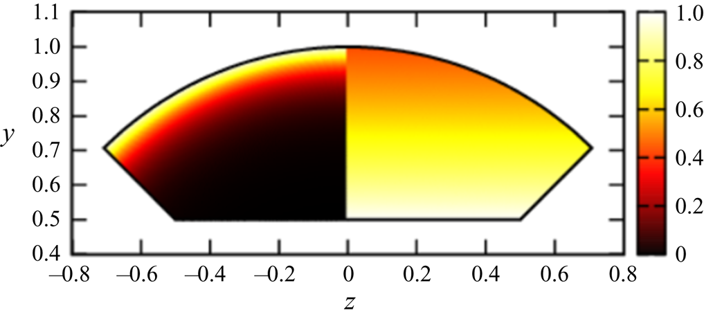
Consider a flow through a duct of a cross-section  $\varOmega$, which is bounded by
 $z=1/2, r=1, \theta ={\rm \pi} /4$ and
 $\theta =3{\rm \pi} /4$; see figure 1. Here the cylindrical coordinates
 $(r,\theta )$ in the
 $y,z$ plane are defined by
 $z=r\cos \theta , y=r\sin \theta$. We assume that the base velocity profile develops a boundary layer near
 $r=1$ so that
 \begin{equation} \bar{u}=u_0\frac{\textrm{e}^{\alpha (r-1)}-\textrm{e}^{-\alpha/2}}{1-\textrm{e}^{-\alpha/2}}. \end{equation}
The parameter  $\alpha$ controls the strength of the shear in the boundary layer, and
 $u_0$ specifies the velocity range (note that
 $\bar {u}\in [0,u_0]$). We use
 $u_0=0.5$ and
 $\alpha =15$ throughout the paper.
The model base flow introduced in § 2.3. Here,  $\alpha =15$,
 $g=1$. The flow profile is symmetric with respect to the
 $z=0$ axis. In the left half of the domain, the normalised base shear
 $\bar {u}/u_0$ is plotted, while the right half is the base density
 $\bar {\rho }$. The applied magnetic field is uniform and the fluid is isothermal.

The fluid is assumed to be isothermal, and subjected to a downward uniform gravity field  $G=-gz$ and a uniform streamwise magnetic field. Here,
 $g$ is a positive constant representing the strength of gravity. Without loss of generality, we can normalise the flow so that the sound-wave speed becomes unity. The density profile
 $\bar {\rho }=\textrm {e}^{\gamma g ({1}/{2}-z)}$ can be found by solving the magnetostatic condition with
 $\bar {\rho }|_{z={1}/{2}}=1$.
The square of the Alfvén wave speed is inversely proportional to the density as
 \begin{equation} a^2=\frac{2}{\gamma \beta_0}\,\textrm{e}^{\gamma g (z-{1}/{2})}.\end{equation}
Here,  $\beta _0$ is the plasma beta (the ratio of the kinematic pressure to the magnetic pressure) at
 $z=\frac {1}{2}$. The cusp wave speed can be computed by (3.20) using (2.14) and
 $s^2=1$. Owing to the normalisation we applied, when
 $u_0$ is less than unity, the base velocity field becomes subsonic everywhere in
 $\varOmega$.
The buoyancy frequency can be found from (2.12):
 \begin{equation} N_1^2=0,\quad N_2^2=g^2(\gamma-1),\quad N_{12}^2=0. \end{equation}
Hereafter, when  $N_1^2+N_2^2>0$ everywhere in
 $\varOmega$, we say that the base flow is convectively stably stratified. For the standard choice
 $\gamma =5/3$ we adopt, clearly the model flow satisfies this condition. The parameters in the model flow are
 $g$ and
 $\beta _0$. The parameter
 $g$ can be used to control the strength of the stratification, while the inverse of
 $\beta _0$ represents the magnitude of the square of the applied magnetic field (thus, small
 $\beta _0$ implies that the applied magnetic field is strong, and vice versa).
In this paper, numerical stability analysis of the model flow is not considered because the numerical study of non-planar flows is far beyond the scope of this study. Here, we shall briefly explain why such a numerical computation is so challenging. First, it is well known that the eigenvalue computation is quite unstable for inviscid problems. The convergence of the iterative methods is not very efficient because of a bad condition number, while in the direct methods, an accurate computation is difficult owing to the singularities that appear in the neutral solutions. Even for unstable eigenmodes, the numerical growth rates are typically not so large, and very sharp structures occur in the corresponding eigenmodes. This is particularly problematic in the non-planar problems because the very high resolution required makes the matrix size huge. For the planar cases, the shooting method is a prescription for this problem but, of course, it is not applicable for the non-planar problems.
To see how the bounds and eigenvalues compare, it is sufficient to use planar flows, as we will see in § 5. Even if we could perform non-planar calculations, we would not obtain much useful information, as our interest is not in studying a particular flow.
3. Semicircle-type theorems
If the flow is assumed to be independent of  $y$ and the gravitational field is uniform, our flow configuration reduces to that considered by Adam (Reference Adam1978b), where the equation for
 $\tilde {q}$ is used to derive a semicircle theorem for convectively stable or neutrally stable flows. Unfortunately, it turns out that the same strategy cannot work for the generalised flow configuration considered in this paper. The issue here can nevertheless be resolved by simply going back to the earlier work of Eckart (Reference Eckart1963), who used the displacement form of the equations. We shall see that there is a close relationship between the well-known energy principle theory for the displacement and the semicircle theorem, which even allows for much refinement of the eigenvalue bound.
3.1. Usual semicircle theorem
Let us begin our analysis by briefly reviewing the energy principle theory that forms the basis of the derivation of the semicircle theorem. The energy balance, in terms of the Lagrange description, can be analysed by first taking the inner product of (2.11) and the complex conjugate of the displacement vector, and then integrating it by parts over the domain  $\varOmega$.
 \begin{equation} c^2\langle Q \rangle -2c\langle \bar{u}Q \rangle -\delta W=0.\end{equation}
Here
 \begin{equation} Q\equiv \bar{\rho} k^2(|\xi|^2+|\eta|^2+|\zeta|^2), \end{equation}
is positive definite, and the angle brackets represent the integration over the domain. The first term, the second term and the third term on the left side of (3.1) are referred to as the kinematic energy, gyroscopic term and potential energy, respectively. The last term  $\delta W$ is, of course, from the force operator
 $\boldsymbol {F}$. Bernstein et al. (Reference Bernstein, Frieman, Kruskal and Kulsrud1958) showed that for the static case (
 $\bar {u}=0$), the base state is stable if and only if
 $\delta W$ is positive definite, while in the presence of the shear (
 $\bar {u}\neq0$), the positiveness only guarantees the sufficient condition of the stability (Frieman & Rotenberg Reference Frieman and Rotenberg1960). These properties immediately follow by solving the quadratic equation (3.1) for
 $c$.
The terms in (3.1) can be rearranged to obtain the following form that is more suitable to obtain the semicircle theorem:
 \begin{equation} \langle U^2Q \rangle=\langle \mathcal{L} \rangle.\end{equation}
The integral appearing on the right side is  $\langle \mathcal {L}\rangle =\delta W+\langle \bar {u}^2Q \rangle$ and the explicit form of
 $\mathcal {L}$ can be found by (2.8b), (2.8c) and (2.9) as
 \begin{align} \mathcal{L}&= \bar{\rho}s^2|ik \xi+\eta_y+\zeta_z|^2 +\bar{\rho}a^2\{k^2 (|\eta|^2+ |\zeta|^2)+|\eta_y+\zeta_z|^2\} \nonumber\\ &\quad +\bar{\rho}\{(G_y\eta+G_z\zeta)^*(ik \xi+\eta_y+\zeta_z)+(G_y\eta+G_z\zeta)(ik \xi+\eta_y+\zeta_z)^*\}\nonumber\\ &\quad +(G_y\eta+G_z\zeta)^*(\bar{\rho}_y\eta+\bar{\rho}_z\zeta) \nonumber\\ &=\bar{\rho}s^2|ik \xi+\eta_y+\zeta_z+s^{{-}2}(G_y\eta+G_z\zeta)|^2 +\bar{\rho}a^2|\eta_y+\zeta_z|^2 \nonumber\\ &\quad +\bar{\rho}\{ (N_1^2+k^2a^2)|\eta|^2 +(N_2^2+k^2a^2)|\zeta|^2 +N_{12}^2(\zeta^*\eta+\eta^*\zeta)\}. \end{align}
Note that  $Q$ and
 $\mathcal {L}$ are real-valued functions. Thus the real and imaginary parts of (3.3) become
 \begin{gather} \langle \{(\bar{u}-c_r)^2-c_i^2\} Q \rangle=\langle \mathcal{L} \rangle, \end{gather}
 \begin{gather}-2c_i\langle (\bar{u}-c_r) Q \rangle=0, \end{gather}
respectively.
First we show that the semicircle theorem holds for unstable modes ( $c_i\neq 0$), as long as
 $\langle \mathcal {L}\rangle \geq 0$ is satisfied, and then check when the latter condition is satisfied. As is usual for Howard-type theory, we combine (3.5) with the obvious inequality
 \begin{equation} \left\langle \left(\bar{u}-min_{\varOmega}\bar{u}\right) \left(\bar{u}-max_{\varOmega}\bar{u}\right)Q \right\rangle = \langle \{\bar{u}^2-2\bar{u}_+c_r+\bar{u}_+^2-\bar{u}_-^2\}Q \rangle \leq 0,\end{equation}
where
 \begin{equation} \bar{u}_\pm{\equiv} \tfrac{1}{2} \left(max_{\varOmega}\bar{u}\pm min_{\varOmega}\bar{u}\right). \end{equation}
Noting that (3.6) now implies  $\langle \bar {u}Q \rangle =c_r \langle Q \rangle$, so we have
 \begin{equation} \langle \{(c_r-\bar{u}_+)^2+c_i^2\}Q \rangle \leq \langle \bar{u}_-^2Q\rangle, \end{equation}
which is nothing but the semicircle theorem  $(c_r-\bar {u}_+)^2+c_i^2 \leq \bar {u}_-^2$ ensuring that in the complex plane, the unstable eigenvalue
 $c$ lies inside, or on, the semicircle in the upper half-plane, whose centre and radius are
 $\bar {u}_+$ and
 $\bar {u}_-$, respectively.
There is a simple condition to guarantee  $\langle \mathcal {L}\rangle \geq 0$. The terms in the curly bracket in the last line of (3.4) can be written in a quadratic form:
 \begin{equation} [\eta,\zeta] \left[ \begin{array}{cc} N_1^2+k^2a^2 & N_{12}^2\\ N_{12}^2 & N_2^2+k^2a^2 \end{array} \right] \left[ \begin{array}{c} \eta\\ \zeta \end{array} \right]. \end{equation}
As is well known, the definiteness of the Hermitian quadratic form can be found by the eigenvalues of the matrix; hence,  $\mathcal {L} \geq 0$ must hold if the eigenvalues of the above real symmetric matrix are non-negative for all points
 $y,z$. The eigenvalues are found as
 $k^2a^2$ and
 $k^2a^2+N_1^2+N_2^2$, noting the identity
 $N_{12}^4=N_1^2N_2^2$ (see (2.2) and (2.12)). Therefore, the only caveat in using the semicircle theorem is that
 $k^2a^2+(N_1^2+N_2^2)$ is positive everywhere. In particular, when the flow is not convectively unstably stratified (i.e. if
 $N_1^2+N_2^2\geq 0$ is satisfied at all points in
 $\varOmega$), the semicircle theorem holds for any wavenumber
 $k$.
The result here extends the semicircle theorem for quite general flow configurations, which include those studied by Eckart (Reference Eckart1963) and Adam (Reference Adam1978b). This new result is already remarkable, but note that the derivation above might not be so surprising because, for ideal fluids, the force operator  $\boldsymbol {F}$ in (2.11) typically possesses the self-adjoint property, which is all we need to show that
 $\mathcal {L}$ in (3.3) is purely real. The more substantive findings of this paper will be shown in the next section, where we shall see that the energy principle equation allows us to improve the semicircle bound.
3.2. Inner envelope theorem
The main tool to be used to improve the eigenvalue bound is the simple identity
 \begin{align} \langle\{\bar{u}^2-2\bar{u}c_r+c_r^2-c_i^2\}Q \rangle &=\langle\{ (\bar{u}-r_c)^2 +2\bar{u}(r_c-c_r) +c_r^2-r_c^2 -c_i^2\}Q \rangle \nonumber\\ &=\langle\{ (\bar{u}-r_c)^2 -(c_r-r_c)^2 -c_i^2\}Q \rangle \end{align}
that holds for an arbitrary real number  $r_c$. Here (3.6) is used in the second equality. Equation (3.5) can thus be transformed into
 \begin{equation} \langle \{(c_r-r_c)^2+c_i^2\} Q \rangle=\langle (\bar{u}-r_c)^2 Q \rangle-\langle \mathcal{L} \rangle. \end{equation}
If we can find a positive number  $R(r_c)$, such that
 \begin{equation} \langle (\bar{u}-r_c)^2 Q \rangle-\langle \mathcal{L} \rangle\leq R^2\langle Q\rangle,\end{equation}
we can establish a semicircle theorem with the centre  $r_c$ and the radius
 $R(r_c)$. The theory works for any real number
 $r_c$, and hence the net eigenvalue bound in the complex plane can be obtained by drawing the semicircles changing
 $r_c$.
Here we shall make a few remarks on the relationship between the new eigenvalue bound and the usual semicircle bound. First, if  $\langle \mathcal {L}\rangle = 0$, namely if the flow is unstratified, incompressible and non-magnetised, the best bound found by (3.12) coincides with the usual semicircle. This can be easily checked by noticing
 $min_{\varOmega }(\bar {u}-r_c)=\bar {u}_+-\bar {u}_--r_c$ and
 $max_{\varOmega }(\bar {u}-r_c)=\bar {u}_++\bar {u}_--r_c$. Then the inequality
 $\langle (\bar {u}-r_c)^2 Q \rangle \leq (|\bar {u}_+-r_c|+|\bar {u}_-|)^2\langle Q \rangle$ implies that the semicircles for any
 $r_c$ contain the usual semicircle. Second, if
 $\langle \mathcal {L}\rangle > 0$, the usual semicircle can be found by the choice
 $r_c=\bar {u}_+$ that enables us to use
 $R=\bar {u}_-$ from the trivial inequality
 $\langle (\bar {u}-\bar {u}_+)^2 Q \rangle -\langle \mathcal {L} \rangle < \langle (\bar {u}-\bar {u}_+)^2 Q \rangle \leq \bar {u}_-^2 \langle Q\rangle$. One may notice that this choice of
 $R$ might be not optimal because the property of
 $\langle \mathcal {L}\rangle$ is not used except for its positiveness. In fact, the reason why the envelope semicircle theorem below gives a better bound is that it uses that property more effectively.
Of course, to draw a bound in the complex plane, we must somehow find  $R(r_c)$ that satisfies (3.13). The best possible eigenvalue bound could be found by seeking the optimum value of
 $R^2$ for all possible displacement functions:
 \begin{equation} R^2\equiv max_{\xi,\eta,\zeta} \frac{\langle (\bar{u}-r_c)^2Q-\mathcal{L}\rangle}{\langle Q \rangle},\end{equation}
where the value of  $R^2$ may be able to be found by treating the Euler–Lagrange equations as an eigenvalue problem for eigenvalue
 $R^2$ (see § B of the supplementary material for details). However, this method is not practically very useful, because the computational effort to solve this eigenvalue problem is comparable to that for the stability problem. Furthermore, we may need to check if the stationary point found by the Euler–Lagrange equations is really a maximum, considering the second variational problem.
There is an alternative way to estimate  $R$ that satisfies (3.13) analytically. Because ease of computation is an advantage in applying the bounds to practical problems, in this paper we focus on this method. We first note that by introducing an arbitrary positive function
 $\sigma (y,z)$, the integrand
 $\mathcal {L}$ seen in (3.4) can be rewritten in the form
 \begin{align} \mathcal{L}&= \bar{\rho}\left\{\sigma \left|\eta_y+\zeta_z+\frac{ik s^2\xi+G_y\eta+G_z\zeta}{\sigma}\right|^2+(s^2+a^2-\sigma)|\eta_y+\zeta_z|^2\right\} \nonumber\\ &\quad + \bar{\rho}\boldsymbol{\xi}^{{{\dagger}}}(k^2\mathbb{L}_2+k \mathbb{L}_1+\mathbb{L}_0)\boldsymbol{\xi}, \end{align}
where  $\boldsymbol {\xi }$ is the transpose of
 $[i\xi ,\eta ,\zeta ]$ and
 \[ \mathbb{L}_2 = \left[ \begin{array}{ccc} s^2\left(1-\dfrac{s^2}{\sigma}\right) & 0 & 0 \\ 0 & a^2 & 0 \\ 0 & 0 & a^2 \end{array} \right], \quad \mathbb{L}_1=\left(1-\frac{s^2}{\sigma}\right) \left[ \begin{array}{ccc} 0 & G_y & G_z \\ G_y & 0 & 0 \\ G_z & 0 & 0 \end{array} \right],\]
 \[ \mathbb{L}_0= \left[ \begin{array}{ccc} 0 & 0 & 0 \\ 0 & \dfrac{G_y\bar{\rho}_y}{\bar{\rho}}-\dfrac{G_y^2}{\sigma} & \dfrac{G_z\bar{\rho}_y}{\bar{\rho}}-\dfrac{G_yG_z}{\sigma} \\ 0 & \dfrac{G_z\bar{\rho}_y}{\bar{\rho}}-\dfrac{G_yG_z}{\sigma} & \dfrac{G_z\bar{\rho}_z}{\bar{\rho}}-\dfrac{G_z^2}{\sigma} \end{array} \right], \]
are real symmetric matrices. The eigenvalues of  $\mathbb {L}_1$ and
 $\mathbb {L}_0$ can be worked out analytically as
 \begin{gather} \left\{0,\left(1-\dfrac{s^2}{\sigma}\right)\sqrt{G_y^2+G_z^2}\}, -\left(1-\dfrac{s^2}{\sigma}\right)\sqrt{G_y^2+G_z^2} \right\}, \end{gather}
 \begin{gather}\left\{0,0,\dfrac{G_y\bar{\rho}_y+G_z\bar{\rho}_z}{\bar{\rho}}- \dfrac{G_y^2+G_z^2}{\sigma}\right\}, \end{gather}
respectively. The new form of  $\mathcal {L}$ suggests that as long as
 $0< \sigma \leq s^2+a^2$ holds everywhere, the terms in the curly bracket in (3.15) are positive definite, and thus we can drop them in the estimation of the radius
 $R$.
Now suppose at each  $y,z$, the largest eigenvalues of the matrices
 $(\bar {u}-r_c)^2\mathbb {I}-\mathbb {L}_2$,
 $-\mathbb {L}_1$,
 $-\mathbb {L}_0$ are calculated (
 $\mathbb {I}$ is a 3 by 3 identity matrix); we denote them as
 $\lambda _2(y,z)$,
 $\lambda _1(y,z)$,
 $\lambda _0(y,z)$, respectively. Then if
 $0<\sigma \leq s^2+a^2$ everywhere, from (3.12) and (3.15), we can deduce
 \begin{align} &\langle \{(c_r-r_c)^2+c_i^2\}Q \rangle \leq k^2 \langle \bar{\rho}\boldsymbol{\xi}^{{{\dagger}}}\{(\bar{u}-r_c)^2\mathbb{I}- \mathbb{L}_2-\lambda_2\mathbb{I}\}\boldsymbol{\xi} \rangle \nonumber\\ &\qquad +k \langle \bar{\rho}\boldsymbol{\xi}^{{{\dagger}}}\{-\mathbb{L}_1 -\lambda_1\mathbb{I}\}\boldsymbol{\xi} \rangle +\langle \bar{\rho}\boldsymbol{\xi}^{{{\dagger}}}\{-\mathbb{L}_0- \lambda_0\mathbb{I}\}\boldsymbol{\xi} \rangle \nonumber\\ &\qquad +\langle (\lambda_2+k^{{-}1}\lambda_1+k^{{-}2}\lambda_0) Q\rangle \nonumber\\ &\quad \leq \langle (\lambda_2+k^{{-}1}\lambda_1+k^{{-}2}\lambda_0) Q\rangle \leq R^2\langle Q \rangle, \end{align}
where we have defined the radius  $R$ so that
 \begin{equation} R^2\equiv max_{\varOmega}(\lambda_2+k^{{-}1}\lambda_1+k^{{-}2}\lambda_0), \end{equation}
where  $R^2$ is, of course, dependent on our choice of the function
 $\sigma$. Optimising this function so that we have the tightest possible bound (see § C of the supplementary material), we have the following theorem.
Theorem 3.1 The unstable complex phase speed  $c=c_r+ic_i$ of (2.5) is bounded so that
 $(c_r-r_c)^2+c_i^2\leq \{R(r_c)\}^2$ for any real number
 $r_c$. Here, the radius
 $R$ is determined by
 $R^2=max_{\varOmega }\lambda (y,z)$, where
 \[\lambda(y,z)= \left\{
\begin{array}{@{}ll}
(\bar{u}-r_c)^2-c_T^2max\left(1-\dfrac{k_h}{k},0\right) &
\text{if }N_1^2+N_2^2\geq 0,\\
\begin{aligned} &
(\bar{u}-r_c)^2-c_T^2\left(1-\dfrac{k_h}{k}\right)\\
& \quad
+max\left(\dfrac{N_{1a}^2+N_{2a}^2}{k_h^2},0\right)max\left(1-\dfrac{k_h}{k},0\right)\\
& \quad-min\left(\dfrac{N_{1a}^2+N_{2a}^2}{k^2},0\right)
\end{aligned} & \text{otherwise}. \end{array} \right. \]
Here we have defined the magnetic buoyancy frequencies
 \begin{equation} N_{1a}^2\equiv \frac{G_y\bar{\rho}_y}{\bar{\rho}}-\frac{G_y^2}{s^2+a^2},\quad N_{2a}^2\equiv \frac{G_z\bar{\rho}_z}{\bar{\rho}}-\frac{G_z^2}{s^2+a^2}, \end{equation}
the local cusp (tube) wave speed
 \begin{equation} c_T\equiv \sqrt{\frac{s^2a^2}{s^2+a^2}},\end{equation}
and the wavenumber  $k_h\equiv h^{-1}$ associated with the density scale height
 \begin{equation} h\equiv \frac{s^2}{\sqrt{G_y^2+G_z^2}}. \end{equation}
A notable property of this new bound is that it works without any caveat; recall that the usual semicircle theorem works only when  $\langle \mathcal {L}\rangle \geq 0$. Therefore, from the theorem, an eigenvalue bound can be deduced even when the flow is strongly unstably stratified. When the flow is not convectively unstably stratified
 $(N_1^2+N_2^2\geq 0)$ everywhere in
 $\varOmega$, the bound should become tighter than the usual semicircle bound because of the term
 $c_T^2max(1-{k_h}/{k},0)\geq 0$ in the function
 $\lambda (y,z)$ (recall that if this term is absent, we have the usual semicircle bound). Owing to the stabilisation, the radius
 $R(r_c)$ can become zero at some
 $r_c$, in which case we can establish the stability of the flow. This is another feature that has not been seen in the usual semicircle theorem.
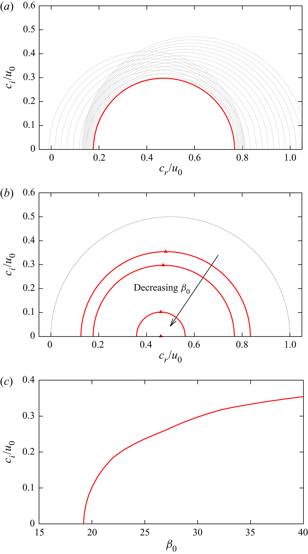
Here we use the model flow defined in § 2.3 to see how such a bound/stability condition can be deduced from the above theorem. Figure 2(a) demonstrates the derivation of the net eigenvalue bound for  $\beta _0=30$. The thin grey circles are the semicircles with various choices of
 $r_c$. We can easily compute the radius
 $R(r_c)$ of them by maximising the quantity
 $\lambda$ over
 $\varOmega$. Then, since the eigenvalues must lie within the semicircle for any
 $r_c$, the net bound can be found by taking the inner envelope of the semicircles, as shown by the thick red curve in the figure. Recall that the model flow is convectively stably stratified. Thus, as remarked above, the inner envelope bound should become tighter than the semicircle theorem. This can be confirmed in figure 2(b), where the inner envelope bounds for
 $\beta _0=19.2, 20,30,40$ are shown by the red curves. The red triangles on the bounds show the maximum
 $c_i$ attained by the corresponding bound. The variation of that maximum with respect to
 $\beta _0$ is shown in figure 2(c). As the
 $\beta _0$ decreases, the bound becomes tighter, which indicates the stabilising effect of the applied magnetic field. We can show why this happens using the explicit form of the bound. As the applied magnetic field becomes stronger, the cusp wave speed
 $c_T$ increases, and hence the aforementioned term
 $c_T^2max(1-{k_h}/{k},0)\geq 0$ representing the stabilisation effect becomes more dominant. It is clear from figure 2(c) that when
 $\beta _0$ is smaller than
 $19.2$, the inner envelope bound predicts the stability of the flow.
Eigenvalue bounds by Theorem 3.1 for the model flow defined in § 2.3. Here,  $(k,u_0,g)=(10, 0.5, 1)$. (a) Derivation of the net eigenvalue bound. The thin grey curves are the semicircles for various choices of
 $r_c$ for
 $\beta _0=30$, and the red thick curve is their inner envelope (i.e. the net eigenvalue bound). (b) Comparison of the inner envelope bounds for
 $\beta _0=19.2,20,30,40$. The triangles indicate the maximum
 $c_i$ attained in each bound. The thin dotted circle is the usual semicircle bound. (c) Variation of the the maximum
 $c_i$ predicted by the inner envelope bound.

A similar stabilisation effect by the applied magnetic field was reported in some previous unstratified incompressible planar flow studies, and they are in fact included in our result. The incompressible limit  $s\rightarrow \infty$ implies
 $k_h\rightarrow 0$ and
 $c_T\rightarrow a$. Therefore, we simply have
 $R^2=max_{\varOmega }\{(\bar {u}-r_c)^2-a^2\}$, where the term proportional to the square of the Alfvén wave speed essentially describes the stabilisation effect for example found by Howard & Gupta (Reference Howard and Gupta1962). More specifically, we can show that the incompressible, unstratified and planar version of our result contains the two bounds found by Hughes & Tobias (Reference Hughes and Tobias2001). If we set
 $r_c=0$, our bound becomes
 $c_r^2+c_i^2\leq max_{\varOmega } (\bar {u}^2-a^2)$, which is identical to (3.10) in Hughes & Tobias (Reference Hughes and Tobias2001). If we set
 $r_c=\bar {u}_+$, the bound becomes
 $(c_r-\bar {u}_+)^2+c_i^2\leq max_{\varOmega } ((\bar {u}-\bar {u}_+)^2-a^2)$, from which we can deduce
 $(c_r-\bar {u}_+)^2+c_i^2\leq \bar {u}_-^2-min_{\varOmega } a^2$, namely (3.14) of Hughes & Tobias (Reference Hughes and Tobias2001). Gupta (Reference Gupta1992) treated the incompressible version of our non-planar system but, as remarked by Cally (Reference Cally2000), there are some errors. The corrected bound is essentially the second bound in the paper by Hughes & Tobias (Reference Hughes and Tobias2001).
A crucial difference between the above incompressible results and our compressible stratified result is that whether the stabilisation occurs or not depends on the wavenumber owing to the term proportional to  $k_h/k$ in
 $\lambda (y,z)$. For the convectively stable flows, in the limit of
 $k_h/k\rightarrow 0$, the bound becomes tightest and Cally's stability condition derived for unstratified flows can be recovered; the flow is stable if there exists a Galilean frame in which the flow nowhere exceeds the cusp speed. (This can be easily checked by noting our expression of the radius becomes
 $R^2=max_{\varOmega }\{(\bar {u}-r_c)^2-c_T^2\}$ in the limit; Cally (Reference Cally2000) considered planar flows but from the result here clearly his stability condition can be carried over to non-planar flows.) However, the stabilisation does not occur at all if
 $k$ is smaller than
 $k_h$, namely, when the wavelength is larger than the density scale height, the bound becomes the usual semicircle. As an example, consider the model flow used in figure 2 again. The wavenumber associated with the density scale height is
 $k_h=g=1$. The reason why we had effective magnetic stabilisation in figure 2 is that the wavenumber
 $k=10$ we used is much larger than
 $k_h$. For
 $k\leq 1$, the ratio
 $k_h/k$ is greater than unity and thus the net bound is merely the usual semicircle irrespective of the value of
 $\beta _0$. Theorem 3.1 implies that, somewhat counter-intuitively, the presence of the stable stratification may hinder the stabilisation effect by the applied magnetic field.
The behaviour of the bound for the unstably convectively stratified flows is more complicated, but at least it is easy to check that when there is no velocity shear, the bound is consistent with the sufficient condition of stability reported by Newcomb (Reference Newcomb1961) (note that Newcomb (Reference Newcomb1961) also deduced the necessary condition of stability). To check this, we may set  $(\bar {u}-r_c)^2=0$ in our bound. The sign of
 $\lambda (y,z)$ can be easily found in table 1 of the paper by Newcomb (Reference Newcomb1961). If
 $0\leq N_1^2+N_2^2$, clearly,
 $\lambda (y,z)\leq 0$ and thus
 $R^2\leq 0$ for all
 $k$. This sufficient condition of stability is precisely what was shown by Newcomb (Reference Newcomb1961), though it is now extended for the general conservative force field. In § 5, we will examine the bound for a specific convectively unstable shear flow.
Finally, we briefly comment on the stability condition derived by Adam (Reference Adam1978a), who also used the energy principle theory assuming a planar base field depending only on  $z$. His method is essentially based on the minimisation problem of
 $\delta W=\langle \mathcal {L}-(\bar {u}-r_c)^2Q\rangle$. If it is positive for all possible displacements, as remarked at the beginning of this section, the flow must be stable (see Frieman & Rotenberg Reference Frieman and Rotenberg1960). The displacement vector that gives the stationary value of
 $\delta W$ could be found by the Euler–Lagrange equations. Adam (Reference Adam1978a) used those equations to eliminate the two displacement components from the stationary value of
 $\delta W$ and make it a function of only one remaining displacement component. However, there is a flaw in this key step towards his stability condition. His Euler–Lagrange equations almost always do not have a solution other than the trivial one
 $(\xi =\eta =\zeta =0)$. Thus the stationary value of
 $\delta W$ is merely zero (which makes sense because
 $\delta W$ can be written in a quadratic form), and thus the sign of it does not supply a meaningful stability condition. Moreover, the second variational problem considered in that paper treats variations of only two displacement components, and the consideration of this problem does not guarantee that the stationary point is a minimum for all possible displacements.
Here one might notice that Adam's method has some similarity to the method mentioned just below (3.14) and section B of the supplementary material. The optimisation problem (3.14) resembles what was considered by Adam (Reference Adam1978a), but the crucial difference is that, in our method,  $\delta W$ is normalised by
 $\langle Q \rangle$, which is essentially the norm of the displacement. This normalisation makes the stationary value non-trivial and produces a Lagrange multiplier
 $R^2$ in our Euler–Lagrange equations. Therefore, the error of Adam (Reference Adam1978a) essentially comes from the fact that he assumed the existence of a non-trivial Euler–Lagrange solution associated with the eigenvalue
 $R^2=0$, which is almost always impossible.
The derivation of the stability conditions by Tobias & Hughes (Reference Tobias and Hughes2004) is based on the theory by Adam (Reference Adam1978a) and, hence, is not correct as well. Therefore, there is no simple stability condition available for the flows influenced by shear, stratification, compressibility and magnetic field, except for that deduced in Theorem 3.1.
4. Generalisation of the Miles–Howard theory, the semi-ellipse type theorem, and Cally's eigenvalue bound
Our primary aim of this section is to generalise the Miles–Howard theory. There are three effects to be included: the compressible; magnetohydrodynamic; and non-planar effects. The conclusion to be deduced in § 4.1 is that, unfortunately, two of these effects prevent the derivation of a stability condition. However, the equations obtained in the course of the analysis are nevertheless useful, because they help us to derive two other types of eigenvalue bounds.
The first bound is somewhat similar to the semi-ellipse theorem of Kochar & Jain (Reference Kochar and Jain1979) derived for planar flows, although it is important to remark here that their derivation is not applicable when the base flow depends on two variables. The alternative idea of using the Lagrangian displacement is motivated by Fung (Reference Fung1986) but, as remarked in § 1, his analysis was not complete. The second bound is similar to that derived by Cally (Reference Cally1983). Again, we note that the method used in that paper cannot be used for non-planar flows, because it is based on the theory by Warren (Reference Warren1970) for certain second-order ordinary differential equations. Thus, our analyses in §§ 4.2 and 4.3 are not merely a minor extension of the previous works but involve new methodologies.
4.1. The Miles–Howard theory for the generalised flow
Following Miles (Reference Miles1961) and Howard (Reference Howard1961), we rescale the perturbation quantities by  $U^{1/2}$. The governing equations for the rescaled displacement
 $\varphi =U^{1/2}\xi$,
 $\phi =U^{1/2}\eta$,
 $\psi =U^{1/2}\zeta$ can be found from (2.8b), (2.8c) and (2.9) as
 \begin{gather} U^{1/2}\tilde{q}={-}\bar{\rho}a^2\hat{\kappa}-(s^2\bar{\rho}(ik\varphi+ \hat{\kappa})+\bar{\rho}\hat{\mathcal{G}}), \end{gather}
 \begin{gather}\bar{\rho}k^2 U^2 \varphi ={-}ik (s^2\bar{\rho}(ik\varphi+\hat{\kappa})+\bar{\rho}\hat{\mathcal{G}}), \end{gather}
 \begin{gather}k^2\bar{\rho}U^{{-}1}(U^2-a^2) \phi=U^{{-}1/2}\tilde{q}_y +U^{{-}1}G_y(\bar{\rho}_y\phi+ \bar{\rho}_z\psi+\bar{\rho}(ik\varphi+\hat{\kappa})), \end{gather}
 \begin{gather}k^2\bar{\rho}U^{{-}1}(U^2-a^2) \psi=U^{{-}1/2}\tilde{q}_z +U^{{-}1}G_z( \bar{\rho}_y\phi+\bar{\rho}_z\psi+\bar{\rho}(ik\varphi+\hat{\kappa})). \end{gather}
For the sake of simplicity, here we have denoted
 \begin{gather} \hat{\mathcal{G}}=G_y\phi+G_z\psi, \end{gather}
 \begin{gather}\hat{\kappa}=U^{1/2}(\eta_y+\zeta_z)= \hat{\kappa}_1-U^{{-}1}\hat{\kappa}_2, \end{gather}
 \begin{gather}\hat{\kappa}_1=\phi_y+\psi_z,\quad \hat{\kappa}_2=\tfrac{1}{2}(U_y\phi+U_z\psi). \end{gather}
Next, we multiply  $\phi ^*$ and
 $\psi ^*$ by (4.1c) and (4.1d) respectively, and then add them together. Integrating the resultant equation by parts over the domain, and taking the imaginary part, we can find that the unstable mode must satisfy (see § D of the supplementary material)
 \begin{equation} 0=\left\langle Q_1+\frac{\hat{f}_b}{|U|^2}-\frac{\bar{\rho}| \hat{\kappa}_2|^2}{|U|^2}\left(\frac{s^2}{|U|^2+s^2}+\frac{a^2}{|U|^2}\right) \right\rangle.\end{equation}
Here
 \begin{align} Q_1&\equiv \bar{\rho}\left(1+\frac{a^2}{|U|^2} \right)k^2(|\phi|^2+|\psi|^2) \nonumber\\ &\quad +\bar{\rho}s^2\frac{|U|^2+s^2}{|U^2-s^2|^2}\left|\hat{\kappa}_1- \frac{2U_r}{|U|^2+s^2}\hat{\kappa}_2+\frac{\hat{\mathcal{G}}}{s^2}\right|^2 +\bar{\rho}\frac{a^2}{|U|^2}\left|\hat{\kappa}- \frac{2U_r}{|U|^2}\hat{\kappa}_2\right|^2, \end{align}
is a real positive function ( $U_r=\bar {u}-c_r$ is the real part of
 $U$) and
 \begin{equation} \hat{f}_b\equiv \frac{G_y}{\bar{\rho}_y}|\bar{\rho}_y\phi+ \bar{\rho}_z\psi|^2-\frac{\bar{\rho}}{s^2}|\hat{\mathcal{G}}|^2,\end{equation}
denotes the buoyancy related terms. Equation (4.3) plays the central role in the Miles–Howard theory. Clearly, in view of this equation, instability is not possible when  $\hat {f}_b-\bar {\rho }|\hat {\kappa }_2|^2({s^2}/({|U|^2+s^2})+{a^2}/{|U|^2})$ is positive everywhere, and this is satisfied if
 \begin{equation} \hat{f}_b-\bar{\rho}|\hat{\kappa}_2|^2\left(1+\frac{a_M^2}{c_i^2} \right)\geq 0,\quad a_M^2\equiv max_{\varOmega}a^2.\end{equation}
Meanwhile let us turn off the external magnetic effect ( $a=0$) to focus on the effect of the non-planar base flow configuration on the Miles–Howard stability condition. From (4.6), the stability of the flow is guaranteed if
 \begin{equation} \frac{\hat{f}_b}{\bar{\rho}}-|\hat{\kappa}_2|^2=[\phi^*, \psi^*] \left[ \begin{array}{cc} \bar{u}_y^2(J_1-\dfrac{1}{4}) & \bar{u}_y\bar{u}_z(J_{12}-\dfrac{1}{4}) \\ \bar{u}_y\bar{u}_z(J_{12}-\dfrac{1}{4}) & \bar{u}_z^2(J_2-\dfrac{1}{4}) \end{array} \right] \left[ \begin{array}{c} \phi\\ \psi \end{array} \right]\end{equation}
is non-negative everywhere in  $\varOmega$. Here, we have defined the generalised Richardson numbers
 \begin{equation} J_1\equiv \frac{N_1^2}{\bar{u}_y^2},\quad J_2\equiv \frac{N_2^2}{\bar{u}_z^2},\quad J_{12}\equiv \frac{N_{12}^2}{\bar{u}_y\bar{u}_z}.\end{equation}
The two eigenvalues  $\lambda _+,\lambda _-$ of the matrix in (4.7) are found as
 \begin{equation} \lambda_{{\pm}}=\frac{(\bar{u}_y^2+\bar{u}_z^2)(J-\frac{1}{4})\pm \sqrt{(\bar{u}_y^2+\bar{u}_z^2)^2(J-\frac{1}{4})^2-\bar{u}_y^2 \bar{u}_z^2(2J_{12}-J_1-J_2)}}{2}, \end{equation}
where
 \begin{equation} J\equiv \frac{N_1^2+N_2^2}{\bar{u}_y^2+\bar{u}_z^2}.\end{equation}
Hence, (4.7) is non-negative if  $\lambda _+,\lambda _-\geq 0$, and those conditions are equivalent to the Miles–Howard-like condition
 \begin{equation} J_m\equiv min_{\varOmega}J \geq \tfrac{1}{4}\end{equation}
and
 \begin{equation} J_{12} \geq \frac{J_1+J_2}{2},\end{equation}
which was first noticed by Fung (Reference Fung1986). However, the question left unanswered in that paper is in what specific situation the condition (4.12) is guaranteed.
Here we note that the identity  $J_1J_2=J_{12}^2$ follows from (4.8). This implies that
 $J_{12}$ is the geometric mean of
 $J_1$ and
 $J_2$, which must be smaller or equal to the arithmetic mean
 $(J_1+J_2)/2$. Therefore, (4.12) is achieved only when the equal sign is established. So what does the base flow look like when this condition is met? To answer this question, let us choose a point
 $(y,z)$ in the domain and consider the two local Cartesian coordinates attached to the contours of
 $\bar {u}$ and
 $G$. Let
 $n$ and
 $\nu$ be the coordinates normal to the contours of
 $\bar {u}$ and
 $G$, respectively. Noting that the contours of
 $\bar {\rho }$ and
 $G$ must coincide, owing to (2.3), we have
 \begin{equation} 2J_{12}-J_1-J_2=\frac{J}{\nu_y^2+\nu_z^2} \left\{2\left(\frac{\nu_y}{n_y}\right)\left(\frac{\nu_z}{n_z}\right)- \left(\frac{\nu_y}{n_y}\right)^2-\left(\frac{\nu_z}{n_z}\right)^2 \right\}, \end{equation}
from the definitions of the Richardson numbers and the buoyancy frequencies. Here, the subscripts  $n$ and
 $\nu$ represent the corresponding partial differentiations. The sum of the terms in the curly bracket cannot become positive because the eigenvalues of the matrix associated with the quadratic form are 0 and
 $-2$. This means that if the flow is stably stratified,
 $2J_{12}-J_1-J_2\leq 0$, which is consistent with our aforementioned observation. We are interested in the case
 $2J_{12}-J_1-J_2=0$, because this is the only case when (4.12) is satisfied. When this happens, the terms in the curly bracket in (4.13) must vanish. This is possible only when
 ${\nu _y}/{n_y}={\nu _z}/{n_z}$, namely the contours of
 $\bar {u}$ and
 $G$ are aligned (i.e. the gradients of
 $\bar {u}$ and
 $G$ are parallel and
 $J_1=J_2=J_{12}$). Therefore, the first important conclusion obtained in this section is that when
 $a=0$, the Miles–Howard condition (4.11) guarantees the stability of the flow only when the directions of the shear and the stratification are aligned everywhere in
 $\varOmega$.
The second conclusion we shall derive here is that even if the above shear-stratification aligned condition is met, in the presence of an external magnetised field ( $a\neq ~0$), the Miles–Howard condition (4.11) no longer guarantees the stability of the flow. Now let us assume the shear-stratification aligned condition
 $J_1=J_2=J_{12}$ for everywhere in
 $\varOmega$. We can write the left side of (4.6) in the quadratic form similar to (4.7), and the argument analogues to the non-magnetised case leads to
 $\lambda _+=(\bar {u}_y^2+\bar {u}_z^2)\{J-\frac {1}{4}(1+{a_M^2}/{c_i^2})\}$ and
 $\lambda _-=0$. Recall that there is no unstable eigenvalue
 $c$ that makes
 $\lambda _+$ positive everywhere in
 $\varOmega$. Hence,
 $c_i^2(4J_m-1)\geq a_M^2$ must be satisfied for any unstable modes. Therefore, when
 $J_m>1/4$, we can derive the upper bound of
 $c_i$
 \begin{equation} c_i^2 < \frac{a_M^2}{4J_m-1}.\end{equation}
Clearly, unless the external magnetic field is completely switched off, the stability of the flow cannot be guaranteed.
4.2. Semi-ellipse-type bound
The outcome of § 4.1 can be combined with the semicircle theorem to yield a tighter bound. In this section, we assume that the base flow is convectively not unstably stratified ( $N_1^2+N_2^2\geq 0$ everywhere in
 $\varOmega$).
First, we show that there is an alternative way to find the semicircle theorem. Writing
 \begin{equation} \kappa=\eta_y+\zeta_z, \quad \mathcal{D}=ik \xi+\kappa, \quad \mathcal{G}=(G_y\eta+G_z\zeta), \end{equation}
from (2.8c) and (2.9a), we can deduce
 \begin{equation} \bar{\rho}k^2 U^2 \xi ={-}ik (s^2\bar{\rho}\mathcal{D}+\bar{\rho}\mathcal{G}),\end{equation}
while (2.9b), (2.9c) and (2.8b) become
 \begin{gather} k^2\bar{\rho}(U^2-a^2) \eta=\tilde{q}_y +G_y(\eta \bar{\rho}_y+\zeta \bar{\rho}_z+\bar{\rho}\mathcal{D}), \end{gather}
 \begin{gather}k^2\bar{\rho}(U^2-a^2) \zeta=\tilde{q}_z +G_z(\eta \bar{\rho}_y+\zeta \bar{\rho}_z+\bar{\rho}\mathcal{D}), \end{gather}
 \begin{gather}\tilde{q}={-}\bar{\rho}a^2\kappa-(s^2\bar{\rho}\mathcal{D}+\bar{\rho}\mathcal{G}). \end{gather}
The integration by parts of  $\eta ^*\times$(4.17)
 $+\zeta ^*\times$(4.18) over the domain becomes
 \begin{align} \langle k^2\bar{\rho}(U^2-a^2)(|\eta|^2+|\zeta|^2) \rangle =\langle \mathcal{G}^*(\eta \bar{\rho}_y+\zeta \bar{\rho}_z)+\bar{\rho}(\mathcal{G}^*\mathcal{D}+\kappa^*s^2\mathcal{D}+ \kappa^*\mathcal{G}+a^2|\kappa|^2) \rangle, \end{align}
after eliminating  $\tilde {q}$ using (4.19). Further, using the identities
 $\mathcal {D}=({U^2\kappa +\mathcal {G}})/({U^2-s^2})$ and
 $\mathcal {G}^*\mathcal {D}+\kappa ^*s^2\mathcal {D}+\kappa ^*\mathcal {G}= ({s^2U^2|\kappa +s^{-2}\mathcal {G}|^2})/({U^2-s^2})-{|\mathcal {G}|^2}/{s^2}$ led by (4.16), the integral above can be simplified as
 \begin{equation} \langle U^2Q_2 \rangle =\left\langle \bar{\rho}\frac{s^2|U|^4|\kappa+s^{{-}2}\mathcal{G}|^2}{|U^2-s^2|^2}+f_b+ \bar{\rho}a^2(k^2(|\eta|^2+|\zeta|^2)+|\kappa|^2)\right\rangle.\end{equation}
Here
 \begin{equation} Q_2\equiv k^2\bar{\rho}(|\eta|^2+|\zeta|^2)+\bar{\rho}\frac{s^4|\kappa+ s^{{-}2}\mathcal{G}|^2}{|U^2-s^2|^2}\end{equation}
is a real and positive function, and
 \begin{equation} f_b\equiv U^{{-}1/2}\hat{f}_b = \bar{\rho} [\eta^*, \zeta^*] \left[ \begin{array}{cc} N_1^2 & N_{12}^2 \\ N_{12}^2 & N_2^2 \end{array} \right] \left[ \begin{array}{c} \eta\\ \zeta \end{array} \right] \end{equation}
is the buoyancy related term, which is non-negative for convectively stably stratified flows.
The right side of (4.21) is real and positive, and thus it is in a suitable form to derive a semicircle theorem. The argument similar to § 3.1 can be applied to (4.21), to yield
 \begin{equation} \langle \{\bar{u}_-^2-(c_r-\bar{u}_+)^2-c_i^2-\varTheta\}Q_2\rangle \geq \langle f_b\rangle,\end{equation}
where a real number  $\varTheta$ is introduced to express the possible contraction of the semicircle radius from the usual case. From the inspection of the right side of (4.21), the best choice of
 $\varTheta$ can be found as
 \begin{equation} \varTheta=min_{\varOmega}min \left(a^2, \frac{c_i^4}{s^2}\right). \end{equation}
(When there is no stratification at all ( $G\equiv 0$), there is a better choice
 $\varTheta =min_{\varOmega } min (a^2, c_T^2+({a^2}/{c_T^2})({c_i^4}/{s^2}))$ that can be found by using the identity
 ${|U|^4}/{s^2}+({a^2}/{s^4})|U^2-s^2|^2=c_T^2+(({s^2+a^2})/{s^4})|U^2-c_T^2|^2$, but we will not go into further detail.)
For some eigenvalues, we can estimate  $\langle f_b \rangle$ from below by a positive number, thereby further improving the bound. Relating
 $Q_1$ and
 $Q_2$ appropriately and using (4.3), after some laborious algebra given in § E of the supplementary material, we can find the estimate
 \begin{equation} \langle f_b \rangle \geq \left(J_m\frac{c_i^2}{\mathcal{C}^2}- \frac{\lambda_M}{k^2} \right)\langle Q_2\rangle, \end{equation}
where
 $$\begin{gather} \lambda_M\equiv max_{\varOmega}\frac{\sqrt{(\bar{u}_y^2+\bar{u}_z^2)^2(J-J_m)^2 +4\bar{u}_y^2\bar{u}_z^2J_m(J_1+J_2-2J_{12})}- (\bar{u}_y^2+\bar{u}_z^2)(J-J_m) }{2}, \end{gather}$$
 $$\begin{gather}\mathcal{C}\equiv \frac{1+\sqrt{1+\mu\left(\dfrac{a_M^2}{c_i^2}- 4J_m\right)}}{2\mu}. \end{gather}$$
The estimate (4.26) holds only when
 \begin{equation} \mu \equiv 1-\frac{\lambda_M}{k^2c_i^2}.\end{equation}
is positive; otherwise, we simply use the estimation  $\langle f_b \rangle \geq 0$. The quantity
 $\lambda _M\geq 0$ measures how much the shear and the stratification are not aligned – this is precisely what was missing in the paper by Fung (Reference Fung1986). Combining (4.24) and (4.26), we have the bound
 \begin{equation} (c_r-\bar{u}_+)^2+\left(\mu+\frac{J_m}{\mathcal{C}^2}\right)c_i^2\leq \bar{u}_-^2 -\varTheta. \end{equation}
We also remark that when  $\mu >0$, the argument of the square root appearing in
 $\mathcal {C}$ should be positive (see (4.28)). From this condition, when
 $J_m>\frac {1}{4}$, we can deduce the following upper bound of
 $c_i^2$ (see § F of the supplementary material)
 \begin{equation} c_i^2< \frac{(4J_m k^{{-}2}\lambda_M+a_M^2)+\sqrt{(4J_mk^{{-}2}\lambda_M+a_M^2)^2-4(4J_m-1)k^{{-}2}\lambda_M a_M^2}}{2(4J_m-1)}.\end{equation}
The above results can be summarised in the following theorem.
Theorem 4.1 If  $N_1^2+N_2^2 \geq 0$ everywhere in
 $\varOmega$, the unstable complex phase speed
 $c=c_r+ic_i$ of (2.5) is bounded so that
 \[ (c_r-\bar{u}_+)^2+\varGamma c_i^2 \leq \bar{u}_-^2-min_{\varOmega}min \left(a^2,\frac{c_i^4}{s^2}\right), \]
with
 \[ \varGamma= \left\{ \begin{array}{@{}ll} \displaystyle max\left(1,\mu+4\mu^2J_m \left\{1+\sqrt{1+\mu \left(\dfrac{max_{\varOmega}a^2}{c_i^2}-4J_m\right)}\right\}^{{-}2}\right) & \text{if }\mu>0,\\ 1 & \text{otherwise}, \end{array} \right. \]
where  $J_m=min_{\varOmega }J$ and
 $\mu$ is the quantity defined in (4.29). If
 $J_m>\frac {1}{4}$, the inequality (4.31) must also be satisfied.
The expression of the bound is rather complicated, so it might be worth considering the perfectly shear-stratification-aligned case first (namely  $\lambda _M=0$). For the sake of simplicity, we further assume that the Alfvén and sound speeds are constants. In this case, the bound in Theorem 4.1 can be simplified as
 \begin{gather} (c_r-\bar{u}_+)^2+c_i^2\left\{\frac{4J_m}{\left(1+\sqrt{1+ \dfrac{a^2}{c_i^2}-4J_m}\right)^2}+1\right\} \leq \bar{u}_-^2-min \left(a^2, \frac{c_i^4}{s^2}\right), \end{gather}
 \begin{gather}\text{additionally}\quad c_i^2< \frac{a^2}{4J_m-1}\quad \text{if } J_m>\frac{1}{4}. \end{gather}
To plot the bound in the complex plane, we set  $(a^2,s^2)=(0.025u_0^2,0.1u_0^2)$, where
 $u_0$ is a constant specifying the range of the base velocity (
 $\bar {u} \in [0,u_0]$). The eigenvalue bounds (4.32) for
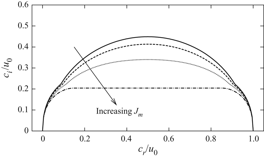
 $J_m=0.1,0.2,0.3,0.4$ are shown in figure 3. We can see that the boundary becomes tighter as the effect of the stratification gets stronger. The bounds for
 $J_m=0.1,0.2$ are determined solely by (4.32a) because
 $J_m\leq \frac {1}{4}$. The dents on the bounds arise from the two possible values of the right side of (4.32a),
 $\bar {u}_-^2-a^2$ and
 $\bar {u}_-^2-c_i^4/s^2$; the middle part of the bound is determined by the former and the near ends by the latter. When
 $J_m>\frac {1}{4}$, we must also consider (4.32b), which is essentially (4.31) for the general case. (Note also that this condition reduces to (4.14) for the perfectly shear-stratification-aligned case.) For
 $J_m=0.3$, the upper bound of
 $c_i/u_0$ predicted by (4.32b) is approximately
 $0.355$, which is well above the bound determined by (4.32a). Thus, for this case, the overall picture of the bound is unchanged from the previous two cases. However, for
 $J_m=0.4$, the upper bound (4.32b) does play a role in the eigenvalue bound. In the figure, the flat top of the bound at
 $c_i/u_0\approx 0.205$ corresponds to this upper bound.
The eigenvalue bound (4.32). The parameters used are  $\bar {u}_+=\bar {u}_-=u_0/2$,
 $a^2=0.025u_0^2$ and
 $s^2=0.1u_0^2$. The solid, dashed, dotted and dot–dashed curves correspond to
 $J_m=0.1,0.2,0.3,0.4$, respectively. The usual semicircle bound is the circle of diameter unity centred at
 $(0.5,0)$.

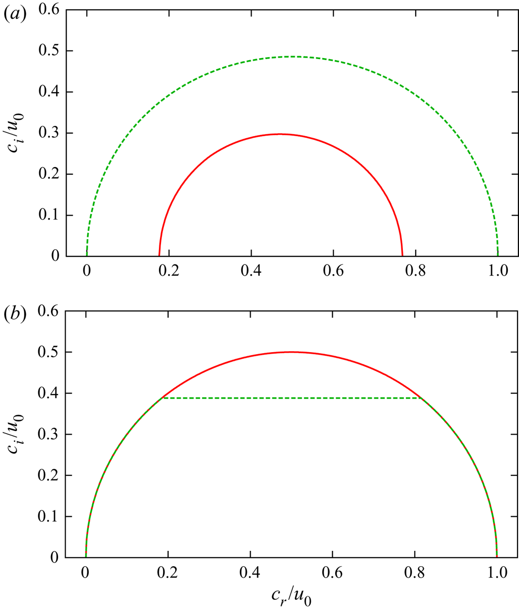
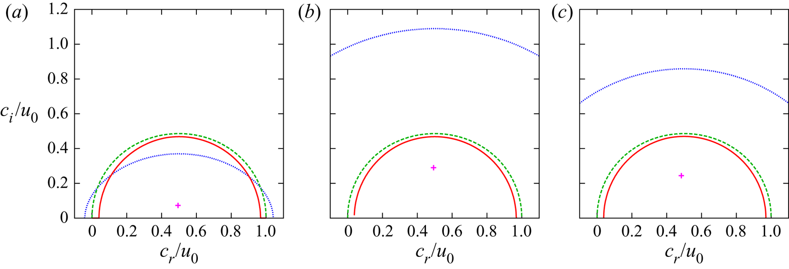
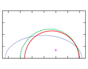
The base flow defined in § 2.3 is a perfect model to study the effect of non-zero  $\lambda _M$, because, as seen in figure 1, the directions of the shear and the stratification are not aligned. Figure 4 shows a comparison of the bounds determined by Theorem 3.1 (red solid) and Theorem 4.1 (green dashed). Figure 4(a) shows the result for the parameters used in figure 2(a),
 $(k,g,\beta _0)=(10,1,30)$. In this case, the inner envelope bound gives a tighter bound than the semi-ellipse-type bound. This is an expected result because the minimum Richardson number of this flow is small (
 $J_m=0.0118$), and so there is not much stabilisation effect by the stratification. In figure 4(b), we changed the parameters to
 $(k,g,\beta _0)=(40,10,10^6)$. The semi-ellipse bound becomes more efficient because the value of
 $g$ is larger than in the previous case and, hence, we have a stronger stable stratification. The minimum Richardson number is
 $J_m=1.18>\frac {1}{4}$ so the upper bound defined by (4.31) appears as the flat top of the boundary. Of course, this upper bound must be small enough to be effective. As seen in the simplified case (4.32b), it is desirable to choose a small magnetic field for this purpose, as we did in figure 4(b). Additionally, to see the effect of the upper bound of
 $c_i$ in the eigenvalue bound,
 $\lambda _M/k^2$ must be sufficiently small. To see this, recall that for the stabilising effect of stratification to appear,
 $\mu =1-\lambda _M/k^2c_i^2$ must be positive. Recall that the semi-ellipse bound is always tighter than the usual semicircle bound and, thus, we have the estimation
 $c_i^2\leq \bar {u}_-^2$. This means that at least the inequality
 $\lambda _M < k^2\bar {u}_-^2$ must hold to see the effect of (4.31); for example, in figure 4(a),
 $\lambda _M=47.1$ and
 $k^2\bar {u}_-^2=100$. An important feature of the non-planar cases is that the stabilising effect of stratification is lost when the wavenumber is small.
The semi-ellipse eigenvalue bounds by Theorem 4.1 for the model flow defined in § 2.3 (green dashed curves). The red solid curves are the inner envelope bounds (Theorem 3.1). Note that both bounds should always fall within the usual semicircle bound (the circle of diameter unity centred at  $(0.5,0)$). (a) The choice of the parameters are
 $(k,u_0,g,\beta _0)=(10, 0.5, 1, 30)$. The semi-ellipse bound is almost the usual semicircle bound because
 $J_m$ is small (
 $J_m=0.0118$ and
 $\lambda _M=0.471$). (b) The choice of the parameters are
 $(k,u_0,g,\beta _0)=(40, 0.5,10,10^6)$, with
 $J_m=1.18$ and
 $\lambda _M=47.1$.

4.3. Outer-envelope-type bound
From the examination of the integral (4.3), clearly
 \begin{equation} \left(1+\frac{a^2}{|U|^2} \right)k^2 (|\phi|^2+|\psi|^2)+\frac{\hat{f}_b}{\bar{\rho}|U|^2}- \frac{|\hat{\kappa}_2|^2}{|U|^2}\left(\frac{s^2}{|U|^2+s^2}+\frac{a^2}{|U|^2} \right)<0,\end{equation}
must be satisfied somewhere in the flow to generate an unstable mode ( $\hat {f}_b$ and
 $\hat {\kappa }_2$ are defined in (4.2), (4.5)). This inequality for the function of
 $(\phi ,\psi ,|U|^2)$ is the key to find alternative proof of the eigenvalue bound derived by Cally (Reference Cally1983). This new method is motivated by Howard (Reference Howard1961), who found a growth rate bound as a byproduct of the derivation of the Miles–Howard condition. The good thing about this alternative approach is that it can be extended to the general non-planar cases as well.
Let us fix  $(y,z) \in \varOmega$. The left-hand side of (4.33) can be written in the quadratic form
 \begin{equation} [\phi^*, \psi^*] \left[ \begin{array}{@{}cc@{}} A+N_1^2-\chi \bar{u}_y^2 & N_{12}^2-\chi \bar{u}_y\bar{u}_z \\ N_{12}^2-\chi \bar{u}_y\bar{u}_z & A+N_2^2-\chi \bar{u}_z^2 \end{array} \right] \left[ \begin{array}{c} \phi\\ \psi \end{array} \right], \end{equation}
using
 \begin{equation} A(|U|^2)=k^2(|U|^2+a^2),\quad \chi(|U|^2)=\frac{(s^2+a^2)(|U|^2+c_T^2)}{4|U|^2(|U|^2+s^2)}. \end{equation}
The eigenvalues of the above matrix are
 \begin{equation} F_{{\pm}}(|U|^2)=A+\tfrac{1}{2}(B\pm \sqrt{B^2+4C}),\end{equation}
where
 \begin{gather} B(|U|^2)=(N_1^2+N_2^2)-\chi (\bar{u}_y^2+\bar{u}_z^2), \end{gather}
 \begin{gather}C(|U|^2)=\chi (\bar{u}_y^2N_2^2-2\bar{u}_y\bar{u}_zN_{12}^2+\bar{u}_z^2N_1^2). \end{gather}
From this result, we see that the inequality (4.33) can be written in the form  $F_+\times (\text {positive quantity})+ F_-\times (\text {positive quantity})<0$. Because
 $F_- \leq F_+$, to have an unstable mode, the inequality
 $F_-(|U|^2)<0$ must be satisfied at least at one point
 $(y,z)$ in
 $\varOmega$.
For sufficiently large  $|U|^2$, the function
 $F_-(|U|^2)$ seen in (4.36) behaves like
 $k^2|U|^2$ and hence it monotonically increases. Now let us denote the largest root of that function as
 $R^2$ (i.e.
 $F_-(R^2)=0$). For
 $|U|^2\geq R^2$, the condition
 $F_-(|U|^2)<0$ cannot be satisfied. Therefore, for any unstable modes, the semicircle-type inequality
 $(\bar {u}-c_r)^2+c_i^2=|U|^2< R^2$ must be satisfied at least at one point
 $y,z$ in the domain.
Theorem 4.2 The unstable complex phase speed  $c=c_r+ic_i$ of (2.5) must satisfy
 \[ (\bar{u}(y,z)-c_r)^2+c_i^2\leq \{R(y,z)\}^2,\]
for some  $(y,z)\in \varOmega$. Here,
 $R^2$ is the largest positive root of
 $F_-(R^2)=0$, where the function
 $F_-$ is defined in (4.36).
This theorem says that the eigenvalues must lie within at least one of the semicircles  $(\bar {u}(y,z)-c_r)^2+c_i^2= \{R(y,z)\}^2$ calculated for various fixed
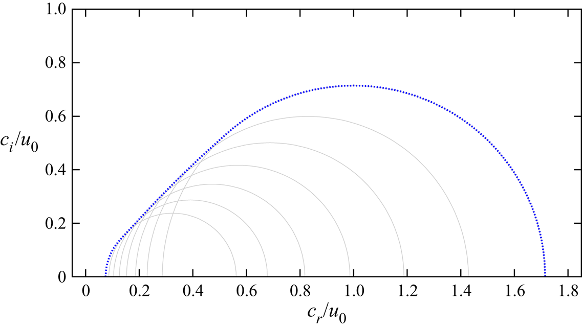
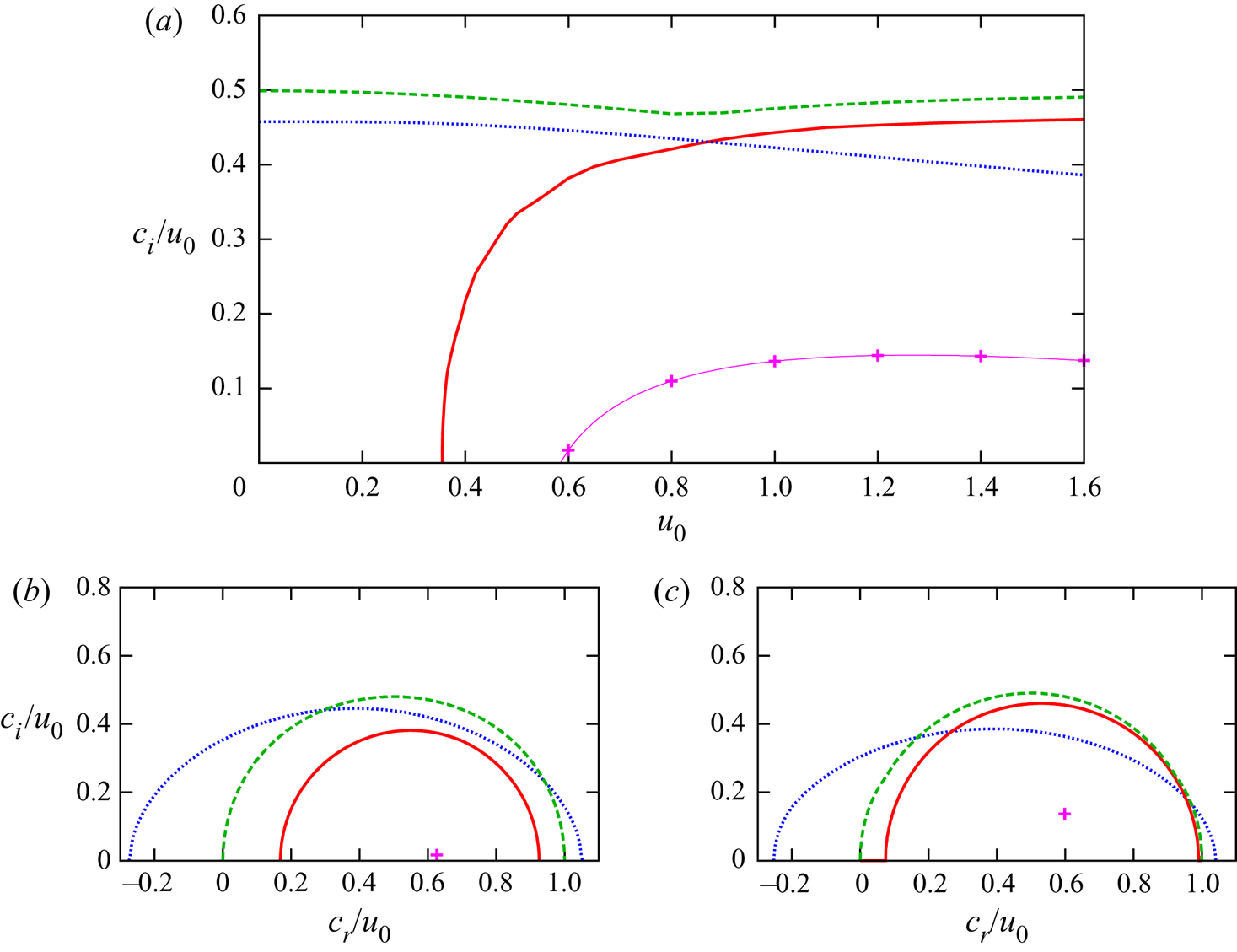
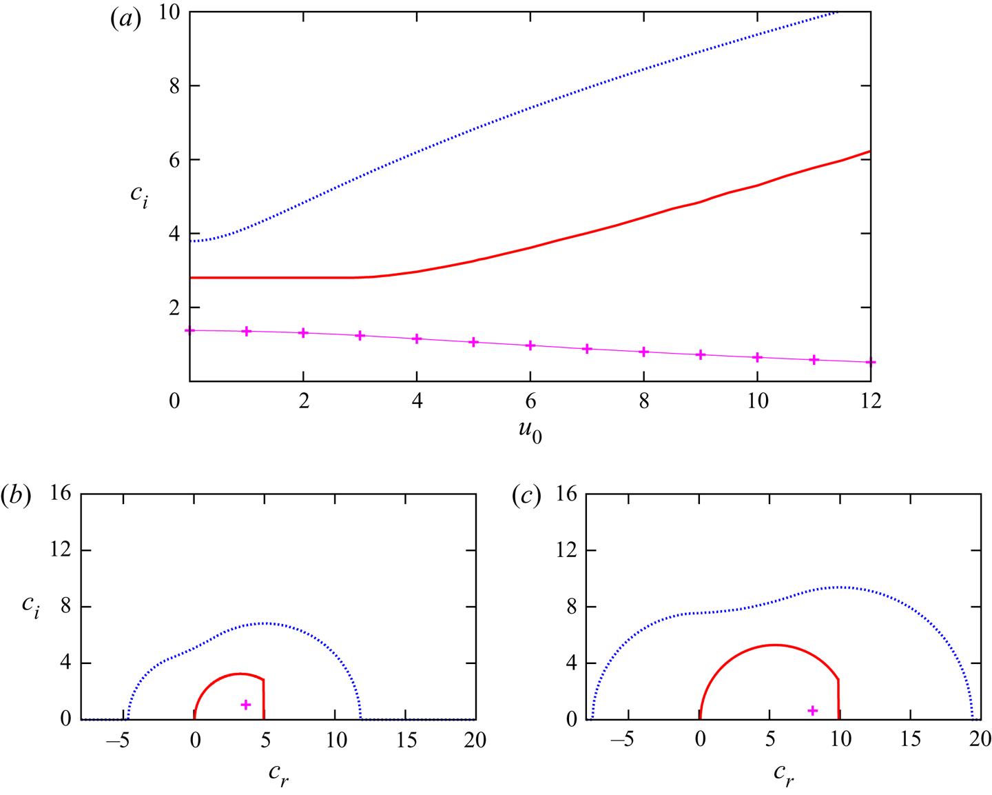
 $(y,z)$. Therefore, in practice, the net eigenvalue bound can be found by plotting the semicircles in the complex plane and taking the outer envelope of them. (Note the difference to Theorem 3.1, where the eigenvalues must lie within all the semicircles.) Figure 5 demonstrates how Theorem 4.2 can be used to construct a net eigenvalue bound for the model flow defined in § 2.3. The parameters in the flow are the same as those used in figures 2(a) and 4(a). The overall property of the outer envelope bound is quite different from the previous two bounds based on the Howard semicircle theory, and thus by using them in a complementary manner, a tighter net bound could be obtained. We will clarify the basic property of the outer envelope bound in the next section.
The eigenvalue bound by Theorem 4.2 for the model flow defined in § 2.3 (blue dotted curve). This is the outer envelope of the grey thin curves, which corresponds to the semicircle-type inequalities for various fixed  $(y,z)$. The choice of the parameters are
 $(k,u_0,g,\beta _0)=(10, 0.5, 1, 30)$. The usual semicircle bound is the circle of diameter unity centred at
 $(0.5,0)$.

It is straightforward to check that the above result is in fact the generalisation of the theory of Cally (Reference Cally1983). When the base field is independent of  $y$, of course
 $C=0$. In this case, the inequality
 $F_-(|U|^2)<0$ reduces to (note that we are only interested in the case
 $B< 0$ where
 $F_-$ may become negative)
 \begin{equation} k^2(|U|^2+a^2)+N_2^2-\frac{(s^2+a^2)(|U|^2+c_T^2)}{4|U|^2(|U|^2+s^2)}u_z^2<0, \end{equation}
which is the inequality (3.19) derived by Cally (Reference Cally1983). In that paper, the perturbations are limited to those that are independent of  $y$ to derive an eigenvalue bound in the complex plane. However, clearly this limitation can be removed from the above result.
As noted by Cally (Reference Cally1983), for non-magnetised cases, the bound reduces to the stability condition by Chimonas (Reference Chimonas1970), who extended the Miles–Howard stability condition for compressible flows. The same argument does not hold for the non-planar flows owing to the existence of the term  $C$, and this is consistent with what we obtained in § 4.1.
5. Comparison of the bounds and numerical eigenvalues
Here we shall compare the eigenvalue bounds obtained so far and the numerical eigenvalues of (2.5). To facilitate the calculation of the eigenvalues of the system, we use simple planar model flow configurations. The advantage of using the planar problems is that the stability problem becomes ordinary differential equations and thus the numerical investigation is not difficult. However, in the general non-planar case, partial differential equations must be used, which makes the calculations much more challenging (see § 2.3). Another motivation for treating the planar problems is to show that the results of this paper contain new findings even for the classical cases.
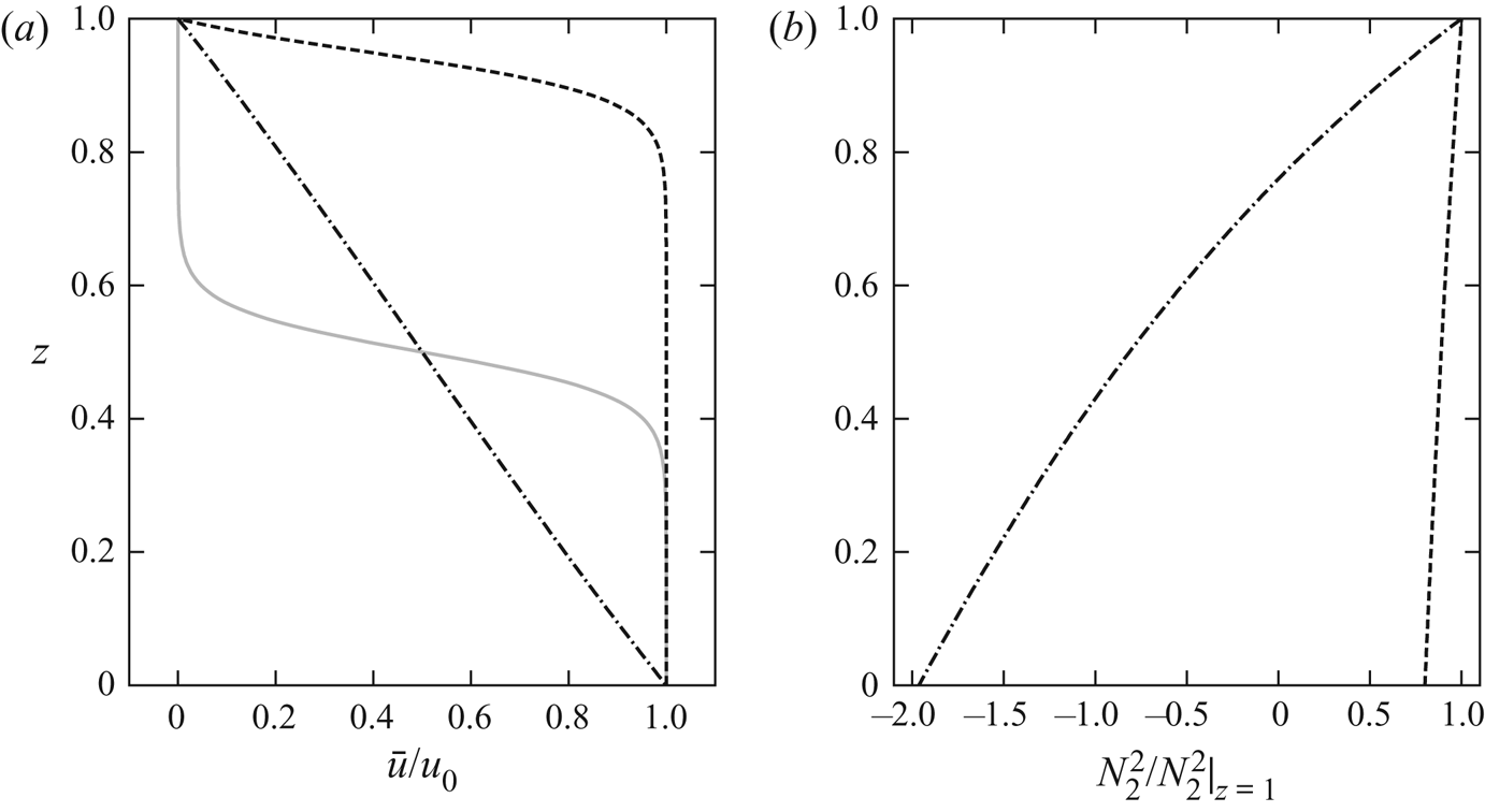
We consider three base flow configurations in a layer  $z\in [0,1]$ subjected to a downward gravity field
 $G=-gz$, as summarised in figure 6. The choice of the adiabatic exponent
 $\gamma$ is 5/3. Because the base flows are not dependent on
 $y$, the
 $y$ dependence of the perturbation can be written by a monochromatic Fourier mode without loss of generality. Here, the perturbation is assumed to be proportional to
 $\exp (ikx+ily-ikct)$ with the spanwise wavenumber
 $l$. The shooting method is used to compute the eigenvalue
 $c$ of (2.5).
The base flows used in the comparison. The grey solid curve in (a) shows the hyperbolic tangent profile (5.1) with  $\alpha =15, z_s=0.5$. This profile is relevant for figure 7, where the polytrope atmosphere with
 $m=3/2$ is used (thus
 $N_2^2=0$). The dashed curve is the same base flow but
 $m=2, z_s=0.95$, which is used in figure 8. The corresponding buoyancy frequency profile is given in (b). The dot–dashed lines in (a,b) are the base profiles used in figure 5 of Tobias & Hughes (Reference Tobias and Hughes2004) and figure 9 of this study.

Let us begin our analysis by introducing the well-known hyperbolic tangent shear profile
 \begin{equation} \bar{u}=u_0\frac{\tanh(\alpha(1-z_s))-\tanh(\alpha(z-z_s))}{\tanh(\alpha(1-z_s))+\tanh(\alpha z_s)}. \end{equation}
This profile produces an inviscid hydrodynamic instability of the Rayleigh (or Kelvin–Helmholtz) type owing to the existence of the inflection point at  $z=z_s$ in the flow. The shear there can be controlled by the parameter
 $\alpha$, while the velocity range is
 $[0,u_0]$. The shear profile (5.1) is considered in a polytropic atmosphere subjected to a uniform external magnetic field. Such an atmosphere has widely been used in various astrophysical magnetoatmospheric problems; see the paper by Bogdan & Cally (Reference Bogdan and Cally1997) and references therein. Here we set
 $\bar {\rho }^{1+1/m}=\gamma \bar {p}$ with the polytrope index
 $m$, choosing the proportional constant so that the sound wave speed
 $s$ at
 $z=0$ becomes unity. The magnetostatic condition
 ${\textrm {d}\bar {p}}/{\textrm {d}z}+g\bar {\rho }=0$ with
 $\bar {\rho }(0)=1$ yields
 \begin{equation} \bar{\rho}=\left(1-\frac{z}{L}\right)^m,\quad \bar{p}= \frac{1}{\gamma}\left(1-\frac{z}{L}\right)^{m+1}. \end{equation}
Here,  $L=({m+1})/{\gamma g}$ and we fix the constant
 $g$ so that
 $L=5$. The squares of the Alfvén and sound wave speeds are found as
 \begin{equation} a^2=\frac{2}{\gamma \beta_0} \frac{1}{\left(1-\dfrac{z}{L}\right)^m}, \quad s^2=\left(1-\frac{z}{L}\right), \end{equation}
where  $\beta _0$ is the plasma beta at
 $z=0$. Using (2.12),
 $N_1^2=0$ and
 \begin{equation} N_2^2=\frac{g}{L-z}\left(m-\frac{m+1}{\gamma}\right). \end{equation}
The control parameters of the flow are  $m, u_0,\alpha , z_s,$ and
 $\beta _0$.
First let us consider the parameters  $(m, u_0,\alpha , z_s, \beta _0)=(3/2,0.5, 15, 0.5, 150)$, setting the rigid boundary conditions at
 $z=0$ and 1. The index
 $m=3/2$ is the special case where the buoyancy frequency
 $N_2^2$ becomes zero everywhere in the flow. The plasma beta of the flow is large, which means that the imposed magnetic field is weak. Thus we expect that the situation is not too far from the usual hydrodynamic unstratified shear flow problem. The inflection point is placed at the middle of the flow domain. The growth rate takes its maximum around
 $k=10, l=0$, and for this case, we compare it with the bounds in figure 7(a). The complex phase speed is normalised by the velocity range
 $u_0$ in the figure so that the usual semicircle bound becomes the circle of diameter unity centred at
 $(0.5,0)$. The phase speed
 $c_r$ of the numerical eigenvalue (magenta cross) is approximately half of
 $u_0$ and, with respect to the
 $c_r/u_0=0.5$ axis, the plot is almost symmetric. As anticipated, the inner envelope bound (Theorem 3.1, the red solid curve) and the semi-ellipse bound (Theorem 4.1, the green dashed curve) are very close to the usual semicircle bound. The blue dotted curve is the outer envelope bound (Theorem 4.2), which now reduces to the bound obtained by Cally (Reference Cally1983). This bound gives a tighter growth rate estimate than the other two bounds in figure 7(a), but it typically becomes looser when the shear is strong or the wavenumber
 $k$ is small (see figure 7(b,c). This property is very similar to the eigenvalue bound (4.1) derived in the paper by Howard (Reference Howard1961); in fact, the Cally-type bound can be reduced to this bound in the absence of the compressibility and the magnetohydrodynamic effect. Next, we introduce some more asymmetry in the flow, changing the inflection point
 $z_s$ to
 $0.95$, and the boundary condition at the top (
 $z=1$) to the free one. Additionally, we select
 $m=2$, so that the buoyancy frequency varies in
 $z$. As shown in figure 6(b), the flow is convectively stably stratified. The maximum growth rate can still be found at
 $l=0$ as is typical for shear dominated instabilities (however, note that Squire's theorem is formally not valid for magnetised problems; see Hunt Reference Hunt1966). The comparison is given in figure 8, where the definitions of the curves and points remain the same as those in figure 7. The magenta crosses in figure 8(a) show how the value of
 $c_i$ changes in the numerical eigenvalue problem when
 $u_0$ is varied; the result is compared with the maximum
 $c_i$ predicted by the bounds. Figures 7(b) and 7(c) are the comparison of the numerical eigenvalues and the bounds in the complex plane at
 $u_0=0.6$ and
 $1.6$, respectively. In figures 7(b) and 7(c), what is immediately apparent is that the inner envelope and Cally-type bounds become largely asymmetric – the property that was not seen in the usual semicircle bound. As the flow is convectively stably stratified, the inner envelope bound becomes tighter than the usual semicircle bound (see § 3.2). The contraction of the bound effectively works because the wavenumber is larger than that associated with the density scale height (
 $k_h \in [0.36, 0.45]$). The semi-ellipse bound is also tighter than the usual semicircle bound but looser than the inner envelope bound, because the stabilisation effect by the stratification is not apparent owing to the strong imposed magnetic field (
 $\beta _0=50$). Turning back to figure 5(a), we can see that for
 $u_0\gtrsim 0.87$, the Cally-type bound gives a tighter bound in terms of
 $c_i$. While for small
 $u_0$, the inner envelope bound gives a better result, which predicts the critical value
 $u_0\approx 0.36$ below which the flow must be stabilised. This critical value is not too far from the numerically determined stability threshold
 $u_0\approx 0.58$ at which the unstable eigenvalue vanishes.
Comparison of the eigenvalues (magenta crosses) and the eigenvalue bounds for the hyperbolic tangent shear profile (5.1) with  $(u_0,\alpha , z_s, \beta _0)=(0.5, 15, 0.5, 150)$. The convectively neutrally stable polytrope atmosphere (
 $m=3/2$) is used. The external magnetic field is uniform. The red solid, the green dashed and the blue dotted curves are the bounds obtained in Theorems 3.1, 4.1 and 4.2, respectively. (a) Result for
 $\alpha =15, k=10,l=0$. The other panels are the same result but in (b) the larger shear parameter
 $\alpha =50$ is used, while in (c) the smaller wavenumber
 $k=4$ is used. Note that the usual semicircle bound is the circle of diameter unity centred at
 $(0.5,0)$.

The eigenvalues and the eigenvalue bounds for the hyperbolic tangent shear profile (5.1) with  $(k,l,\alpha , z_s, \beta _0)=(10,0,15, 0.95, 50)$. The convectively stable polytrope atmosphere with
 $m=2$ is used. The external magnetic field is uniform. The definitions of the curves and the points are the same as figure 7. (a) Comparison of the numerical eigenvalues (magenta crosses) and the upper bounds of
 $c_i$ predicted by Theorems 3.1–4.2. (b) and (c) Comparisons in the complex plane at
 $u_0=0.6$ and
 $1.6$, respectively.

In the third flow configuration, we study the convectively unstable case. For this purpose, we simply employ the model flow configuration studied by Tobias & Hughes (Reference Tobias and Hughes2004) considering the linearly varying magnetic field proportional to  $1+2.8 (1-z)$ and the isothermal atmosphere
 $\bar {p}=({\beta _0}/{2})\bar {\rho }$. Here, the constant
 $\beta _0$ is chosen so that it is the plasma beta of the flow at
 $z=1$. The density profile can be found by the magnetostatic condition
 $0=({\beta _0}/{2})({\textrm {d}\bar {\rho }}/{\textrm {d}z})+g \bar {\rho } +({1}/{2\mu _0})({\textrm {d}\bar {B}^2}/{\textrm {d}z})$ together with the boundary condition
 $\bar {\rho }(1)=1$. For
 $z\gtrsim 0.76$, the flow becomes convectively unstable because the buoyancy frequency
 $N_2^2$ becomes negative; see figure 6(b). Because this phenomenon is caused by the application of a non-uniform magnetic field, it is called magnetic buoyancy instability. The squares of the Alfvén and sound wave speeds are found as
 \begin{equation} a^2=\frac{\{1+2.8 (1-z)\}^2}{\bar{\rho}},\quad s^2=\frac{\gamma \beta_0}{2}. \end{equation}
We employ the shear profile
 \begin{equation} \bar{u}=u_0 \left(\frac{(1-z)^3}{6}-\frac{(1-z)^2}{4}+\frac{13(1-z)}{12} \right), \end{equation}
that was used in figures 4 and 5 in the paper by Tobias & Hughes (Reference Tobias and Hughes2004). This profile is almost linear, but possesses an inflection point at  $z=0.5$; see figure 6(a). The case of
 $u_0=0$ corresponds to the flow studied by Hughes & Cattaneo (Reference Hughes and Cattaneo1987). (In those papers,
 $z$ is pointing downward so that
 $z=0$ and
 $1$ are the upper and lower boundaries, respectively. Thus the shear and magnetic field profiles used there look a bit different from those given above. Note also that the parameters
 $(\delta , \lambda , \tilde {\beta })$ in the paper by Tobias & Hughes (Reference Tobias and Hughes2004) correspond to our
 $(u_0, g, \beta _0/2)$.)
The parameters  $(k,l,g,\beta _0)=(0.32,8,10,5)$ are selected in figure 9(a) so that we have the same flow configuration studied in figure 5 of the paper by Tobias & Hughes (Reference Tobias and Hughes2004). Figure 9(b,c) is the plot in the complex plane at
 $u_0=5,10$. One of the important differences from the previous cases is that the spanwise wavenumber
 $l$ is not zero, and hence the flow configuration is outside the scope of the semicircle theorem of Adam (Reference Adam1978b) and the eigenvalue bound of Cally (Reference Cally1983). A natural question here is whether the usual semicircle theorem deduced in § 3.1, which extends on Adam's result, can be used or not. The answer is no because the quantity
 $k^2a^2+N_2^2$ is not always positive in the flow (see the discussion just below (3.10)). The fact that the theorem actually does not hold can be confirmed by the numerical result shown in figure 6(a), because the numerically obtained
 $c_i$ does not tend to zero as
 $u_0\rightarrow 0$ (this is the reason why we did not use the normalisation by
 $u_0$ in this figure). The semi-ellipse theorem (Theorem 4.1) cannot be used for this model flow as well, because the flow is convectively unstable. Therefore, the only eigenvalue bounds that are available in figure 6 are the inner envelope bound (Theorem 3.1) and the outer envelope bound (Theorem 4.2). These bounds are depicted by the green dashed and red solid curves, respectively, in the figures. Both of them are consistent with the numerical eigenvalues, and the former gives tighter results than the latter.
(a) The same comparison of  $c_i$ as in figure 8(a) but for the flow studied in figure 5 of Tobias & Hughes (Reference Tobias and Hughes2004). The shear profile (5.6) is used with
 $(k,l,g,\beta _0)=(0.32,8,10,5)$. The atmosphere is isothermal and the linearly varying magnetic field generates the magnetic buoyancy instability. (b) and (c) Comparison in the complex plane at
 $u_0=5$ and
 $10$, respectively (see figure 7 for the definitions of the points and the curves).

6. Discussion and conclusions
We have established three new eigenvalue bounds for the ideal instability of compressible stratified magnetoshear flows varying in two transverse directions. The two bounds obtained are the improved/generalised versions of the Howard semicircle theorem, and the other bound is similar to that derived by Cally (Reference Cally1983) for the planar cases. The properties of the bounds were studied by using the model flow through a duct of non-circular cross-section (figure 1).
The first bound, called the inner envelope bound (Theorem 3.1), is based on the energy principle of the Lagrangian displacement and treats the centre of the semicircle as a parameter. By considering the change in the potential energy owing to the Galilean transformations, we can derive the radii of the semicircles  $R(r_c)$ for a given centre
 $r_c$ on the real axis. Because the unstable eigenvalues should lie in the semicircles for any
 $r_c$ in the complex plane, we can grasp the whole picture of the net eigenvalue bound by drawing an inner envelope of them. Unlike the usual semicircle theorem, the inner envelope theory does not require any particular conditions, and hence can be applied even for convectively unstable flows. In the case of convectively stable stratification, the inner envelope theory should give a bound tighter than the semicircle bound, with a novel property that for some cases, the stability of the flow can be established. This stabilisation is essentially the well-known effect by the applied magnetic field, but a notable finding is that for the compressible stratified flows, the stabilisation is effective only when the wavelength is sufficiently smaller than the density scale height.
The main idea used in the first type of bound is so simple that it can be applicable to many other flows. Of particular interest is the extension of the theory to spherical coordinates because such extended theory may have some relevance to the study of solar/planetary atmospheres. For two-dimensional purely hydrodynamic flows, some extensions of the usual semicircle theorem to the spherical coordinates have been attempted in the geophysics community; see the papers by Thuburn & Haynes (Reference Thuburn and Haynes1996) and Sasaki, Takehiro & Yamada (Reference Sasaki, Takehiro and Yamada2012). Another interesting problem would be the stability analysis of viscoelastic flows, where it has been pointed out that there is an analogy to the magnetohydrodynamic problems (Ogilvie & Proctor Reference Ogilvie and Proctor2003).
The second and third types of bounds are deduced by considering the generalisation of the Miles–Howard stability condition. The flow considered in this paper is subjected to a general conservative force field varying in two directions, as was done by Fung (Reference Fung1986). While such a generalisation might seem to complicate the problem at first sight, it actually makes the underlying physical mechanisms clearer. It turned out that even when the effective Richardson number (see (4.10)) is greater than 1/4 everywhere, to guarantee the stability of the flow, the following two conditions must be satisfied: (i) the directions of the shear and the stratification are perfectly aligned; and (ii) there is no external magnetic field. If either of the conditions is not met, only an upper bound of the growth rate can be found. The conclusion obtained for non-magnetised flows is consistent with the observation by Candelier, Le Dizes & Milet (Reference Candelier, Le Dizes and Milet2011), where the stability of a two-dimensional plane Bickley jet is studied. The linear and nonlinear dynamics of flows having a horizontal component of shear under vertical gravity has attracted much attention in hydrodynamic stability studies in recent years (e.g. Chen, Bai & Le Dizes Reference Chen, Bai and Le Dizes2016; Lucas, Caulfield & Kerswell Reference Lucas, Caulfield and Kerswell2017; Facchini et al. Reference Facchini, Favier, Le Gal, Wang and Le Bars2018). An interesting question is what does the upper bound of the growth rate found in this paper imply for those problems. Moreover, the discovery that the Miles–Howard-type stabilisation mechanism might not be so robust in magnetised problems may have some implications for solar physics and engineering problems. For example, the Richardson number in the tachocline is known to be much larger than a quarter (see Cally Reference Cally2000), but it is not surprising that ideal instabilities occur there owing to the numerous magnetic fields present.
The second bound (Theorem 4.1) can be regarded as a generalised version of the semi-ellipse theorem of Kochar & Jain Reference Kochar and Jain1979, which includes the compressible, magnetohydrodynamic and non-planar effects. The basic idea of this bound is to use the integral derived in the generalised Miles–Howard theory to tighten the semicircle bound. A notable feature of the second bound is that, unlike the first bound, it can incorporate the stabilisation effect of stable stratification. However, consistent with the caveat found for the Miles–Howard stability condition, the existence of the shear perpendicular to the direction of the stratification reduces the amount of the improvement on the bound. The existence of a strong applied magnetic field also hinders the improvement, in which case the first bound may give a better result.
The third bound (Theorem 4.2) is a generalisation of the eigenvalue bound found by Cally Reference Cally1983, but here, a quite different approach is used in the derivation. From the generalised Miles–Howard theory, we can deduce an inequality that must be satisfied somewhere in the flow to generate some instability. At each point in the domain, the inequality defines a semicircle region in the complex plane. Because the eigenvalue must lie within one of those semicircles, the net bound can be found by drawing the outer envelope of them. The basic feature of this bound is that it gives a reasonably tight growth rate bound when the wavenumber is not too small and the base shear is not too strong.
The bounds are compared with the numerical eigenvalues of the two canonical planar model flows used in the solar physics community (Bogdan & Cally Reference Bogdan and Cally1997; Tobias & Hughes Reference Tobias and Hughes2004). The first model flow concerns the Kelvin–Helmholtz-type instability in a convectively stable polytrope atmosphere subjected to a uniform magnetic field. As the instability is predominantly generated by the shear, when the base velocity is sufficiently reduced, the growth rate must be suppressed. The inner envelope bound is particularly useful to capture this typical behaviour of the eigenvalue, even leading to a reasonable threshold value of the base velocity below which the flow is stable. In the second model, the magnetic field is non-uniform, and the magnetic buoyancy instability occurs in the flow. For this case, three-dimensional perturbations are more dangerous and interesting, but such perturbations have not been taken into account in the previous complex eigenvalue bound analyses (Adam Reference Adam1978b; Cally Reference Cally1983). Theorems 3.1 and 4.2 derived in this paper successfully give the bounds, which are consistent with the numerical eigenvalues. All the three bounds are dependent on the wavelength of the perturbation, and become less effective when the wavelength is very long. However, this is not really a practical disadvantage because the wavelength does not exceed the size of the system, so we can think of a maximum wavelength. For example, in Theorem 3.1, if we exclude long-wavelength disturbances, the bound should be better than all the previously known results.
As remarked in § 1, an ideal instability of the streak plays a key role in the self-sustaining mechanism of nonlinear coherent structures in turbulent flows (Hall & Smith Reference Hall and Smith1991; Waleffe Reference Waleffe1997; Wang, Gibson & Waleffe Reference Wang, Gibson and Waleffe2007; Hall & Sherwin Reference Hall and Sherwin2010; Deguchi & Hall Reference Deguchi and Hall2014). The streak is essentially the streamwise non-planar mean field, and hence the self-sustaining process has some resemblance to the mean-field theory in magnetohydrodynamics. The corresponding self-sustainment processes of coherent structures in the nonlinear magnetorotational instability, the shear-driven dynamo and the subcritical magnetoshear instability have recently been formulated by Riols et al. (Reference Riols, Rincon, Cossu, Lesur, Longaretti, Ogilvie and Herault2013), Deguchi (Reference Deguchi2019a,Reference Deguchib) and Deguchi (Reference Deguchi2020), respectively. The upper bound on the growth rate obtained in this paper may be useful to estimate how fast the turbulent burst will occur in the magnetohydrodynamic flows. The fact that the stability of the mean field is involved in the sustainment process of coherent structures implies that the results in this study may have some relevance for turbulence control technologies. Dong, Krasnov & Boeck (Reference Dong, Krasnov and Boeck2012) in fact reported that turbulence can be suppressed by controlling the instability of the mean-field via the imposed streamwise magnetic field. The stability condition by the inner envelope theorem may allow us to know when such suppression will be activated.
Finally, we remark that Rayleigh's inflection point theorem is more difficult to apply for the generalised non-planar flows, unlike Howard's semicircle theorem and the Miles–Howard stability theory studied in this paper. This is because the inflection point theorem essentially comes from the conservation of enstrophy that cannot be used for three-dimensional flows (see Arnold Reference Arnold1978; Dowling Reference Dowling1995). It would be worth noting that recently, Deguchi (Reference Deguchi2019c) nevertheless derived a simple condition for the existence of a neutral mode for flows sheared in two directions. This is an extension of the result of Lin (Reference Lin1955), who showed that the inflection point condition can also be used to check the existence of a neutral mode in the classical shear flow problem. The key simplification here is that for neutral perturbations, we only need to analyse the property of the flow around the critical layer at which the wave becomes singular. For compressible, stratified magnetoshear flows the structure of the singular layer is expected to become much more complicated, and so it is of interest to see how the condition should be modified.
Supplementary material
Supplementary material are available at https://doi.org/10.1017/jfm.2021.466.
Acknowledgements
The author wishes to gratefully acknowledge Professor P. Cally for illuminating discussions and his numerical eigenvalue results used in § 5. The useful comments made by the referees should also be acknowledged.
Funding
This work was supported by Australian Research Council Discovery Early Career Researcher Award DE170100171.
Declaration of interest
The authors report no conflict of interest.