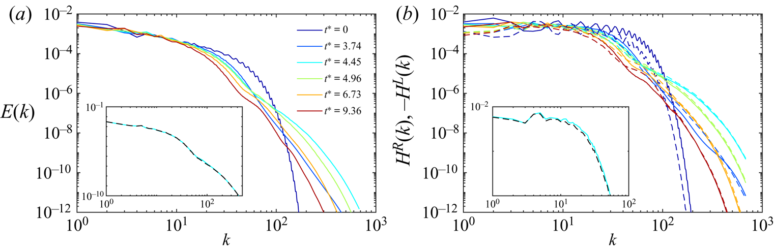
1. Introduction
As a fundamental topology transforming event, reconnection has been extensively studied over recent decades, both in classical (Ashurst & Meiron Reference Ashurst and Meiron1987; Melander & Hussain Reference Melander and Hussain1988; Kida, Takaoka & Hussain Reference Kida, Takaoka and Hussain1991; Kida & Takaoka Reference Kida and Takaoka1994; Hussain & Duraisamy Reference Hussain and Duraisamy2011) and in quantum (Koplik & Levine Reference Koplik and Levine1993; Bewley et al. Reference Bewley, Paoletti, Sreenivasan and Lathrop2008; Zuccher et al. Reference Zuccher, Caliari, Baggaley and Barenghi2012; Fonda, Sreenivasan & Lathrop Reference Fonda, Sreenivasan and Lathrop2019) fluids, as well as in many other subjects, such as plasmas (Priest & Forbes Reference Priest and Forbes2000) and macromolecules (Vazquez & Sumners Reference Vazquez and Sumners2004). It plays a significant role in numerous turbulence phenomena, such as energy cascade (Kivotides et al. Reference Kivotides, Vassilicos, Samuels and Barenghi2001; Yao & Hussain Reference Yao and Hussain2020b), flow transition (Zhao, Yang & Chen Reference Zhao, Yang and Chen2016), fine-scale mixing (Hussain Reference Hussain1986) and noise generation (Daryan, Hussain & Hickey Reference Daryan, Hussain and Hickey2020).
Prior studies on vortex reconnection have mainly focused on relatively simple configurations: vortex rings (Kida et al. Reference Kida, Takaoka and Hussain1991; McKeown et al. Reference McKeown, Monico, Pumir, Brenner and Rubinstein2018), orthogonal vortices or colliding dipoles (Melander & Zabusky Reference Melander and Zabusky1988; Boratav, Pelz & Zabusky Reference Boratav, Pelz and Zabusky1992; Orlandi, Pirozzoli & Carnevale Reference Orlandi, Pirozzoli and Carnevale2012; Jaque & Fuentes Reference Jaque and Fuentes2017), and anti-parallel vortices with a sinusoidal displacement (Pumir & Kerr Reference Pumir and Kerr1987; Melander & Hussain Reference Melander and Hussain1988). Note that reconnection physics of two vortices should be independent of the initial spatial configuration, as two vortex filaments with arbitrary orientations tend to become anti-parallel by mutual induction as they approach each other (Siggia Reference Siggia1985). In general, there are three typical stages of viscous vortex reconnection: inviscid advection, bridging and threading (Melander & Hussain Reference Melander and Hussain1988). During reconnection, extremely small scales can be generated due to vortex stretching; as a result, a sufficiently high resolution is required to capture these structures. Hence, previous direct numerical simulation (DNS) studies of reconnection in classical fluids mainly focused on small-scale problems, such as those with a large core size compared with the domain size and at low to moderate Reynolds numbers (Pumir & Kerr Reference Pumir and Kerr1987; Melander & Hussain Reference Melander and Hussain1988; Shelley, Meiron & Orszag Reference Shelley, Meiron and Orszag1993; Chatelain, Kivotides & Leonard Reference Chatelain, Kivotides and Leonard2003; Kerr Reference Kerr2013). With the rapid development of supercomputers these days, DNS of considerably large-scale problems is becoming feasible (Lee & Moser Reference Lee and Moser2015; Iyer, Sreenivasan & Yeung Reference Iyer, Sreenivasan and Yeung2017). Recent work on vortex reconnection at high Reynolds numbers has revealed more rich phenomena, such as reconnection cascade, where the threads undergo successive reconnections to form secondary vortex rings and a turbulence avalanche (Yao & Hussain Reference Yao and Hussain2020b).
Another type of configuration that has a particular interest is the knotted vortex tube. It has a close relationship to an important quantity: helicity  $H$, which is defined as
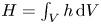 $H=\int _V h\, \mathrm {d}V$, with
 $V$ the entire flow domain and
 $h=\boldsymbol {u}\boldsymbol {\cdot }\boldsymbol {\omega }$ being the helicity density (
 $\boldsymbol {u}$ and
 $\boldsymbol {\omega }$ are the velocity and vorticity, respectively). Helicity measures the degree to which vortex lines embedded in a fluid system wind around each other (Moffatt Reference Moffatt1969; Scheeler et al. Reference Scheeler, van Rees, Kedia, Kleckner and Irvine2017). Similar to energy, helicity is also conserved in ideal fluids and is expected to have a strong influence on the flow evolution. For finite thickness vortex tubes, the helicity can be further geometrically expressed as (Moffatt & Ricca Reference Moffatt and Ricca1992; Scheeler et al. Reference Scheeler, Kleckner, Proment, Kindlmann and Irvine2014)
 \begin{equation} H=\sum_{i \neq j} \varGamma_{i} \varGamma_{j} L k_{i j}+ \sum_{i} \varGamma_{i}^{2}(T_{w,i}+W_{r,i}), \end{equation}
where  $Lk_{i j}$ is the linking number between vortices
 $i$ and
 $j$,
 $W_r$ is the writhe of the vortex centreline and
 $T_w$ is the twist of each vortex. Note that both the linking number and writhe can be obtained from a measurement of the vortex tube centrelines alone; however, the twist and global helicity require additional measurements of the flow inside each of the vortex tubes.
Kida & Takaoka (Reference Kida and Takaoka1987, Reference Kida and Takaoka1988) conducted the first DNS of a trefoil knotted vortex at the vortex Reynolds number  $Re~(\equiv \varGamma /\nu ,\ \mathrm {circulation/viscosity})=1200$ and observed that
 $H$ slowly decreases during the whole process. They further found that the decay rate decreases with increasing
 $Re$, which seems to suggest that
 $H$ is conserved at sufficiently high
 $Re$. Knotted vortex dynamics did not draw too much attention until the work by Kleckner & Irvine (Reference Kleckner and Irvine2013), who experimentally created isolated trefoil knots in water. Using high-speed scanning tomography, they measured the topological and geometrical evolution of these knots and observed an initial stretching of the vortex core, as well as the generation of two separate vortex rings after reconnection. Scheeler et al. (Reference Scheeler, Kleckner, Proment, Kindlmann and Irvine2014) further observed that the centreline helicity is conserved during the topological change from a single trefoil vortex to two separate vortex rings. In addition, they further simulated the evolution of trefoil knots in a superfluid with the Gross–Pitaevskii equation, where a discrete jump in the centreline helicity across the reconnection is observed. Laing, Ricca & Sumners (Reference Laing, Ricca and Sumners2015) analytically demonstrated that total writhe remains conserved under anti-parallel reconnection. Inspired by the studies of Irvine and co-workers, Kerr (Reference Kerr2018c) numerically studied the evolution of perturbed trefoil knotted vortices and confirmed that the total helicity is conserved before reconnection, followed by a progressive and steady decay after reconnection. Scalo and co-workers (Yu, Chapelier & Scalo Reference Yu, Chapelier and Scalo2018; Zhao & Scalo Reference Zhao and Scalo2019) performed large eddy simulations of the trefoil knotted vortex up to
 $Re=20000$ and observed qualitative matches with experiments by Scheeler et al. (Reference Scheeler, Kleckner, Proment, Kindlmann and Irvine2014). Recently, Zhao et al. (Reference Zhao, Yu, Chapelier and Scalo2021) conducted DNS for
 $Re\le 6000$ using the adaptive mesh refinement technique and found that
 $H$ experiences a sudden jump during reconnection at high
 $Re$. Xiong & Yang (Reference Xiong and Yang2019, Reference Xiong and Yang2020) developed a method for constructing knotted vortex tubes with finite thickness, arbitrary complexity and tunable twist, and studied the effect of twist on the evolution in resistive magnetohydrodynamic flows. In addition to these experimental and DNS works, there are also some studies on knotted vortex based on the Biot–Savart model, such as Maggioni et al. (Reference Maggioni, Alamri, Barenghi and Ricca2010) and Oberti & Ricca (Reference Oberti and Ricca2019).
Although reconnection of knotted vortices has been studied both numerically and experimentally, its underlying mechanism remains rather elusive. For example, it is still unclear how helicity affects the reconnection process, whether helicity remains conserved or not, and what is the conversion mechanism between writhe and twist during helicity evolution. These prompted us to conduct a systematic study of the reconnection of trefoil knotted vortices up to  $Re=12\,000$. The paper is organized as follows. In § 2 we provide details of the initial configuration and numerical set-up. The results for zero initial twist (
 $T_{w,0}=0$) cases, including flow visualization, statistics and helicity dynamics, are discussed in §§ 3 and 4. In § 5 the effect of the initial twist on flow evolution is discussed, and, finally, conclusions are drawn in § 6.
2. Initial configuration and numerical set-up
The knotted vortex tube is constructed following Xiong & Yang (Reference Xiong and Yang2019, Reference Xiong and Yang2020). For a given continuous and differentiable closed curve  $C$ without vanishing curvature in three-dimensional Euclidean space
 $\mathbb {R}^3$, its parametric equation is
 $\boldsymbol {x}=\boldsymbol {c}(s)$, where
 $\boldsymbol {x}=(x,y,z)$ denotes spatial Cartesian coordinates and
 $s \in [0, L_C )$ is the arclength parameter with
 $L _C$ the length of
 $C$.
The Frenet–Serret frame on  $C$ is
 \begin{equation} \boldsymbol{T}(s)=\partial_{s} \boldsymbol{c}(s) ; \quad \partial_{s} \boldsymbol{N}=\tau \boldsymbol{B}-\kappa \boldsymbol{T} ; \quad \kappa \boldsymbol{N}=\partial_{s} \boldsymbol{T} ; \quad \partial_{s} \boldsymbol{B}={-}\tau \boldsymbol{N}, \end{equation}
where  $\boldsymbol {T}$,
 $\boldsymbol {N}$ and
 $\boldsymbol {B}\equiv \boldsymbol {T}\times \boldsymbol {N}$ denote the unit tangent, normal and binormal vectors, respectively, and
 $\kappa$ is the curvature and
 $\tau$ is the torsion of the curve. The helicity of the knotted vortex tube can be expressed as
 \begin{equation} H=\varGamma^{2}\left(W_r+T_w\right), \end{equation}
where the writhe (figure 1a) is
 \begin{equation} W_{r}=\frac{1}{4 {\rm \pi}} \oint_{C} \oint_{C} \frac{[\boldsymbol{N}(s) \times \boldsymbol{N}(s^{\prime})] \boldsymbol{\cdot}[\boldsymbol{c}(s)-\boldsymbol{c}(s^{\prime})]}{\left|\boldsymbol{c}(s)-\boldsymbol{c}\left(s^{\prime}\right)\right|^{3}}\, \mathrm{d} s\, \mathrm{d} s^{\prime} \end{equation}
and the twist  $T_w$ can be further decomposed into (Moffatt & Ricca Reference Moffatt and Ricca1992)
 \begin{equation} T_w=T_t+T_i(L_C), \end{equation}
with the total torsion (figure 1b)
 \begin{equation} T_{t}=\frac{1}{2 {\rm \pi}} \oint_{C} \tau\,\mathrm{d} s, \end{equation}
and the intrinsic twist (figure 1c)
 \begin{equation} T_i(s)=\frac{1}{2 {\rm \pi}} \int_{0}^{s} \xi(\lambda) \,\mathrm{d} \lambda. \end{equation}
Here,  $\xi (\lambda )$ is the rate of azimuth change along
 $C$. Note that
 $W_r$ and
 $T_t$ can be uniquely determined once the curve
 $C$ is defined, and their sum is the self-linking number
 $L_s$ (Pohl Reference Pohl1968; Moffatt & Ricca Reference Moffatt and Ricca1992). In addition, the twist
 $T_w$, as well as the total helicity
 $H$, can be tuned by varying the intrinsic twist
 $T_i$. For example, by choosing
 $\xi =-\tau$, one can obtain vortex tubes with zero initial twist
 $T_{w,0}=0$.
Schematics of (a) writhe, (b) torsion twist and (c) intrinsic twist. Adapted from Moffatt & Ricca (Reference Moffatt and Ricca1992) with permission.

Note that for a vortex in viscous flows, it is rather difficult or sometimes even impossible to directly measure its twist  $T_w$. In addition, during vortex reconnection, where numerous fine-scale vortex filaments are generated and become tangled with each other, the helicity decomposition based on (2.2) may break down. As an approximation, we define
 \begin{equation} \tilde{T}_w=H/\varGamma^2-W_r \end{equation}
as ‘generalized twist’.
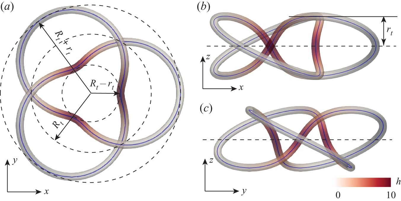
The parametric equations  $\boldsymbol {c}(\zeta )=(c_{x}(\zeta ), c_{y}(\zeta ), c_{z}(\zeta ))$ for the trefoil torus knot (figure 2) are
 \begin{equation} \left. \begin{gathered} \left.c_{x}(\zeta)=\left(R_{t}+r_{t} \cos (q \zeta)\right) \cos (p \zeta)\right), \\ \left.c_{y}(\zeta)=\left(R_{t}+r_{t} \cos (q \zeta)\right) \sin (p \zeta)\right), \\ c_{z}(\zeta)={-}1.5-r_{t} \sin (q \zeta), \end{gathered} \right\} \end{equation}
with  $R_t=1$,
 $r_t=0.5$,
 $p=2$,
 $q=3$ and
 $\zeta \in [0, 2{\rm \pi} )$. Note that
 $R_t$ is also equal to the initial mean radius, defined as
 $\bar {R}=(1/L_c)\oint _{C} R(s)\,\mathrm {d}s$. The writhe
 $W_r$ and the normalized total torsion
 $T_t$ of the curve, calculated based on (2.3) and (2.5), are
 $3.52$ and
 $2.48$, respectively. Hence, the self-linking number
 $L_s=W_r+T_t=6$, which is different from those considered by Scheeler et al. (Reference Scheeler, Kleckner, Proment, Kindlmann and Irvine2014), Kerr (Reference Kerr2018c) and Yu et al. (Reference Yu, Chapelier and Scalo2018) (i.e.
 $L_s=3$).
(a) Top, (b) front and (c) side views of the initial configuration of the trefoil knotted vortex (represented by vorticity isosurface at 4 % of maximum initial vorticity colour coded by the helicity density  $h$). Note that
 $R_t-r_t$ and
 $R_t+r_t$ are the minimum and maximum knot radii, and the blue lines inside the vortex tube denote the vortex centreline.

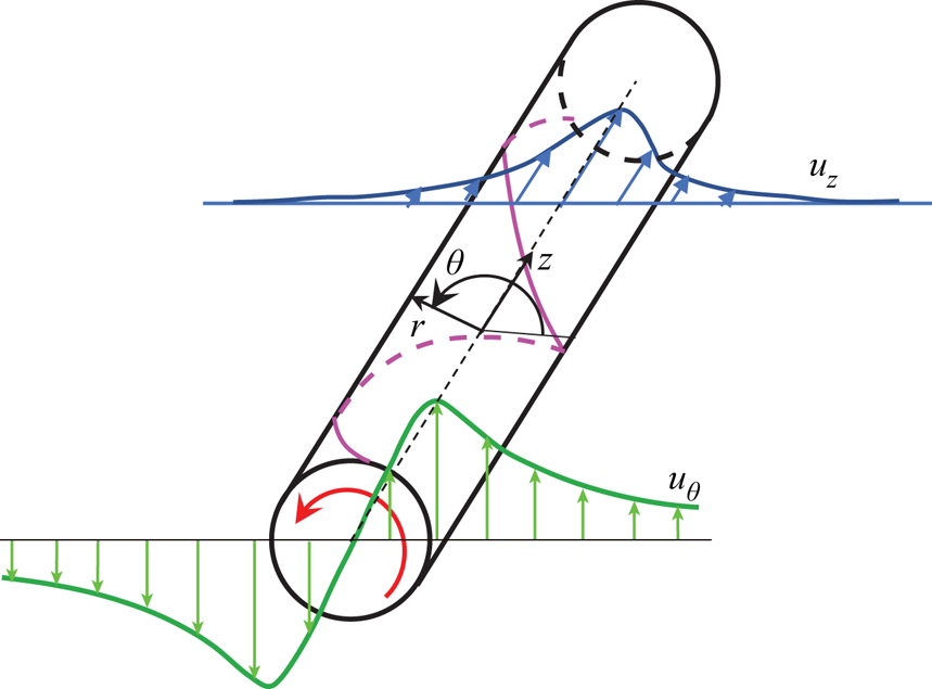
The vorticity field in the curved cylindrical coordinate system is
 \begin{equation} \boldsymbol{\omega}=[\omega_s \boldsymbol{e}_{s} +\omega_\rho \boldsymbol{e}_\rho+\omega_\theta \boldsymbol{e}_{\theta}]= \varGamma f(\rho)\left[\boldsymbol{e}_{s}+\frac{\rho}{1-\kappa \rho \cos \theta}(\xi+\tau) \boldsymbol{e}_{\theta}\right], \end{equation}
where  $\omega _s$,
 $\omega _\rho$ and
 $\omega _\theta$ are the components of
 $\boldsymbol {\omega }$ in the axial (
 $\boldsymbol {e}_{s}$), radial (
 $\boldsymbol {e}_{\rho }$) and azimuthal (
 $\boldsymbol {e}_{\theta }$) directions, respectively;
 $\varGamma$ is the strength of vorticity flux,
 $f(\rho )$ is vorticity flux distribution with
 $\rho$ the nearest distance between the centreline and the point where the vorticity is assigned. Note that the axial component
 $\varGamma f(\rho )\boldsymbol {e}_{s}$ in (2.9) corresponds to the vector field with a writhe-dependent helicity, and the azimuthal part
 $\varGamma f\rho (\xi +\tau ) \boldsymbol {e}_{\theta }/(1-\kappa \rho \cos \theta )$ normal to the central axis represents the twist of vortex lines. The detailed algorithm on how to construct the vorticity field is provided in Xiong & Yang (Reference Xiong and Yang2019, Reference Xiong and Yang2020). In the current study, the strength is set to
 $\varGamma =1$, and the vorticity flux distribution
 $f$ is chosen to be a Gaussian function
 \begin{equation} f(\rho)=\frac{1}{2 {\rm \pi}\sigma^{2}} \exp \left(-\frac{\rho^{2}}{2 \sigma^{2}}\right), \end{equation}
where the standard deviation is set to  $\sigma =1/(16\sqrt {2{\rm \pi} })\approx 0.025$. The effective core radius is estimated as
 $r_e=2\sigma$, within which the vortex tube contains 95 % of the circulation; hence, the ratio between the mean radius and core size
 $R_t/r_e=8\sqrt {2{\rm \pi} }\approx 20$.
Direct numerical simulation of the incompressible Navier–Stokes equations is carried out in a periodic domain with dimensions  $(2{\rm \pi} )^3$ using a Fourier pseudospectral algorithm in the velocity-vorticity form (Pradeep & Hussain Reference Pradeep and Hussain2004; Yao & Hussain Reference Yao and Hussain2020a). Time integration is carried out with an explicit third-order Runge–Kutta scheme, while the viscous term is treated exactly with the integrating factor technique (Canuto et al. Reference Canuto, Hussaini, Quarteroni and Zhang2012). Time is non-dimensionalized as
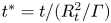 $t^*=t/(R^2_t/\varGamma )$. In the current study, we first consider the zero initial twist cases (
 $\xi =-\tau$) at three different vortex Reynolds numbers
 $Re=2000$,
 $6000$ and
 $12\,000$. In addition, to examine the effect of initial twists, two additional cases with
 $\xi =10{\rm \pi} /L_c$ (
 $T_w=7.48$) and
 $20{\rm \pi} /L_c$ (
 $T_w=22.48$) are considered for
 $Re=2000$ and
 $6000$, respectively. Grid points
 $N^3=768^3$,
 $2048^3$ and
 $4096^3$ are employed for
 $Re=2000$,
 $6000$ and
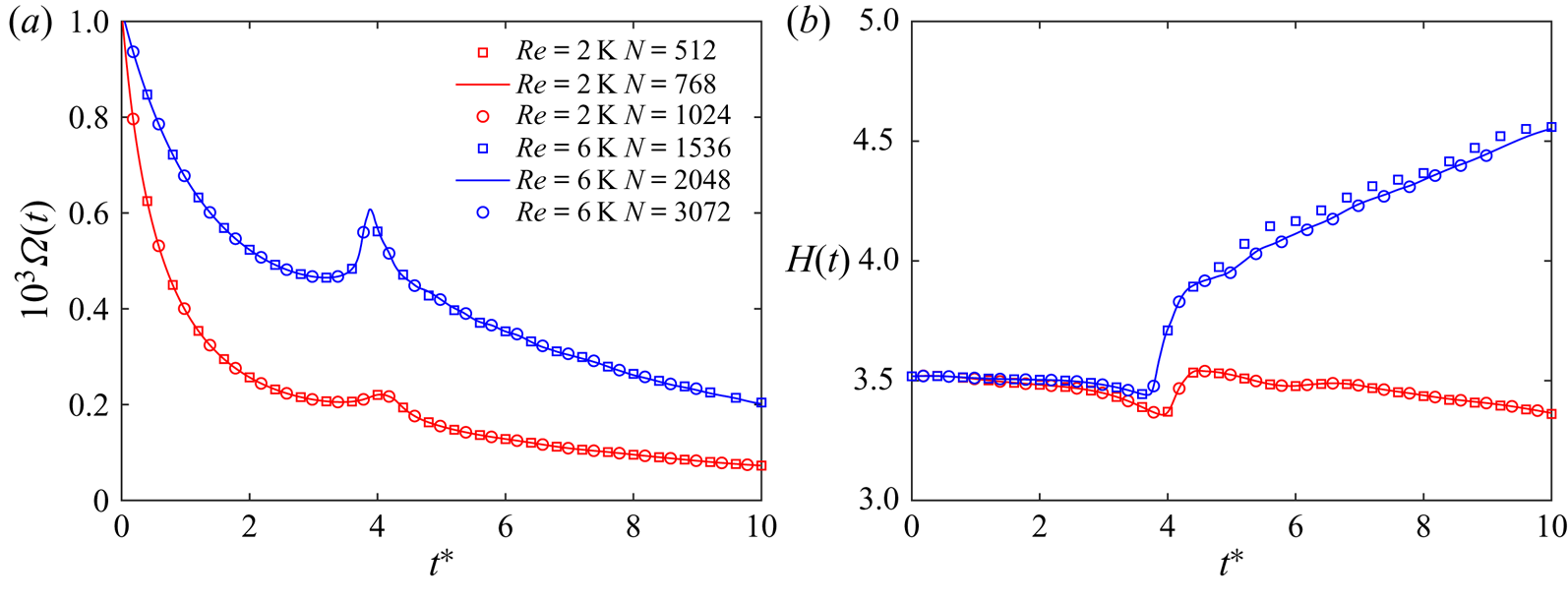
 $12\,000$, respectively. A grid convergence analysis, reported in Appendix A, clearly demonstrates that the grid resolutions employed here are adequate to capture the flow details. Note that due to limited computational resources, the convergence tests are performed only for
 $Re=2000$ and
 $6000$. For
 $Re=12\,000$, the adequacy of the numerical resolution is justified by examining the rate of change of the volume-integrated kinetic energy
 $E=\int _V (\boldsymbol {u}^2/2)\, \mathrm {d}V$ (Archer, Thomas & Coleman Reference Archer, Thomas and Coleman2008; Yao & Hussain Reference Yao and Hussain2020b), whose balance equation for flow in a triply periodic box is
 $\mathrm {d}E/\mathrm {d}t=-2\nu \varOmega ^2$, with
 $\varOmega =\int _V (\boldsymbol {\omega }^2/2) \,\mathrm {d}V$ being the enstrophy. The maximum relative error between
 $|\mathrm {d}E/\mathrm {d}t|$ and
 $2\nu \varOmega ^2$ is less than 1 % – suggesting the adequacy of the numerical resolution.
3. Flow physics for zero initial twist cases
3.1. Flow statistics
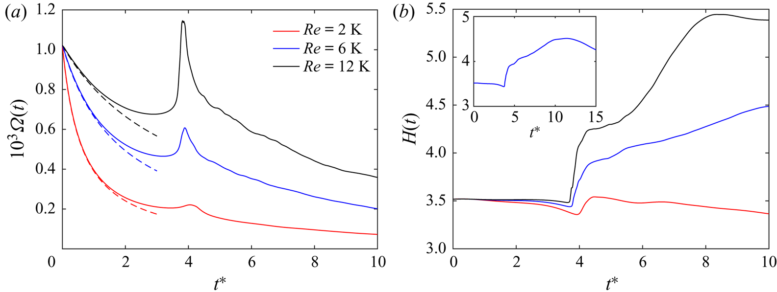
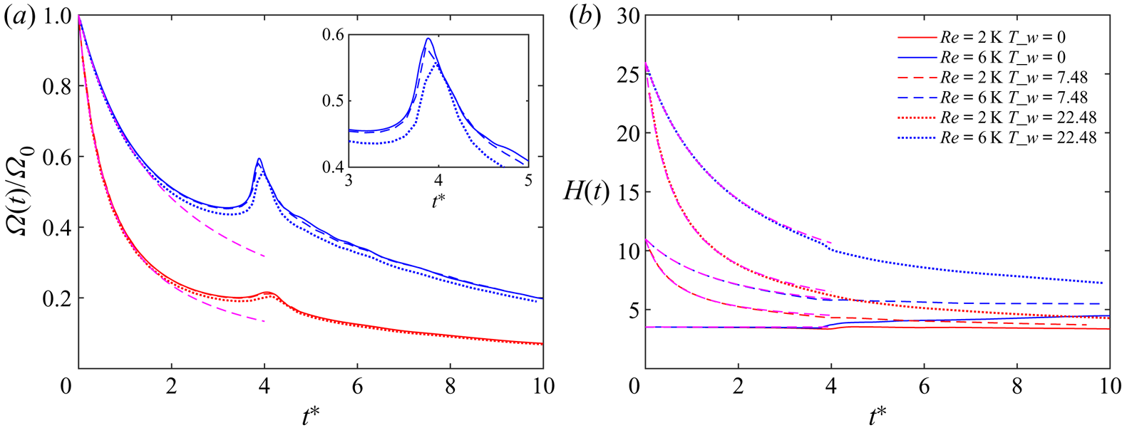
Figure 3(a) shows the time evolution of enstrophy  $\varOmega =\int _V (\boldsymbol {\omega }^2/2)\, \mathrm {d}V$ for three different Reynolds numbers. Due to viscous dissipation, the enstrophy initially decays, and the decay rate decreases with increasing
 $Re$. For a rectilinear Lamb–Oseen vortex, the rate of enstrophy change is
 $(1/\varOmega )\partial \varOmega /\partial t=2\nu /\sigma ^2$ with
 $\sigma$ growing as
 $\sigma (t)= \sqrt {\sigma ^2_0+2\nu t}$ (Appendix B). Consequently, the enstrophy should follow
 $\varOmega (t)=\varOmega _0 \exp [-\int ^t_0(2\nu /\sigma ^2]\,\mathrm {d}t$. For the trefoil vortex considered here, the initial decrease of
 $\varOmega$ also agrees with this prediction, and the agreement deteriorates as
 $Re$ increases – probably due to enhanced enstrophy production caused by vortex stretching. Note that due to smaller vortex core sizes, the enstrophy decays faster than that observed in Yao & Hussain (Reference Yao and Hussain2020b) for thicker core cases. When reconnection occurs,
 $\varOmega (t)$ experiences rapid growth, which also corresponds to an increase in energy dissipation as
 $\epsilon =2\nu \varOmega$. The peak of
 $\varOmega$ increases with
 $Re$, which is due to enhanced vortex stretching and, hence, concomitant higher production. In addition, the time to reach the peak slightly decreases with
 $Re$, suggesting that the reconnection happens sooner at higher
 $Re$ – akin to that observed by Zhao et al. (Reference Zhao, Yu, Chapelier and Scalo2021). Also, the
 $\varOmega$ peak is narrower as the reconnection occurs faster at higher
 $Re$. After the peak, the interaction slows down; as a result, the enstrophy experiences a gradual exponential drop – this time the rate increasing with
 $Re$, because of more numerous and smaller scales created during reconnection.
Time evolution of (a) enstrophy  $\varOmega$ and (b) global helicity
 $H$ for
 $Re=2000$ (red),
 $6000$ (blue) and
 $12\,000$ (black). The dashed lines in (a) denote
 $\varOmega (t)=\varOmega _0 \exp [-\int ^t_0(2\nu /\sigma ^2)]\,\mathrm {d}t$ with
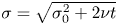 $\sigma =\sqrt {\sigma ^2_0+2\nu t}$, and the inset in (b) shows the long time evolution of
 $H(t)$ for
 $Re=6000$.

The evolution of the global helicity  $H$ is shown in figure 3(b). Initially,
 $H$ remains almost constant, and then slightly decreases before reconnection, with the decay rate decreasing with increasing
 $Re$ due to suppressed viscous dissipation. During and after reconnection, the
 $H(t)$ behaviour is strongly
 $Re$ dependent. At
 $Re=2000$,
 $H$ slowly and steadily decays after a slight increase, which is consistent with the observations by Kida & Takaoka (Reference Kida and Takaoka1987) and Kerr (Reference Kerr2018c). However, at
 $Re=6000$,
 $H$ steadily increases after the jump, which is consistent with the results of Zhao et al. (Reference Zhao, Yu, Chapelier and Scalo2021). Interestingly, such a helicity jump was not clearly observed by Scheeler et al. (Reference Scheeler, Kleckner, Proment, Kindlmann and Irvine2014) and Kerr (Reference Kerr2018c), which might be due to different initial conditions employed in their studies. At
 $Re=12\,000$,
 $H$ rapidly increases and then finally becomes saturated. Compared with its initial value, the peak of
 $H$ for the
 $Re=12\,000$ case increases by approximately 50 %. Note that despite the fact that
 $H$ increases for the two higher
 $Re$ cases after reconnection, it eventually decays. The inset in figure 3(b) provides a longer time evolution of
 $H$ for
 $Re=6000$, showing that
 $H$ starts to decrease at
 $t^*\approx 11.45$. Nevertheless, the transient growth of
 $H(t)$, which is expected to further increase at higher
 $Re$, is quite surprising and will be discussed in detail later.
3.2. Flow structures
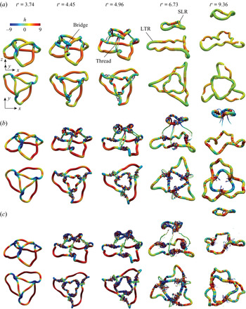
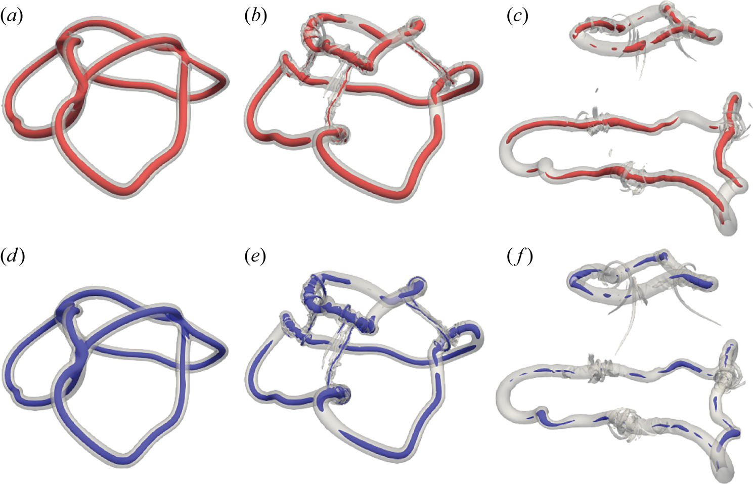
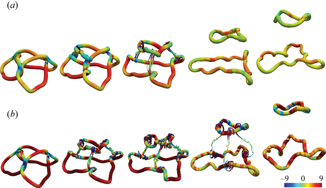
Figure 4 shows the time progression of flow structures visualized based on vorticity magnitude isosurface  $|\boldsymbol {\omega }|$ for different
 $Re$ cases. Note that to capture the evolution details, a relatively low threshold
 $|\boldsymbol {\omega }|=0.04\omega _0$ is chosen, with
 $\omega _0$ being the maximum vorticity magnitude at
 $t^*=0$. The knotted vortex rotates counterclockwise as it moves along the
 $z$-direction. During this process, the vortex is deformed so that the neighbouring parts of the tube become anti-parallel and collide with each other due to self-induction; and then reconnect in a manner similar to previous studies, e.g. Melander & Hussain (Reference Melander and Hussain1988) and Boratav et al. (Reference Boratav, Pelz and Zabusky1992). Due to symmetry, three reconnections occur simultaneously. Note that it is different from those reported by Kleckner & Irvine (Reference Kleckner and Irvine2013) and Kerr (Reference Kerr2018c), where the trefoil knotted vortex is perturbed and only one reconnection occurs at a time. The reconnected parts (called bridges) combine with other parts – forming two separated vortex rings, i.e. a small leading ring and a large trailing ring (hereinafter, referred to as SLR and LTR, respectively). Both SLR and LTR continuously rotate as they propagate upward. Different from quantum reconnection, the viscous reconnection is not complete, and parts of the initial vortex tube are left over as threads. As the two rings propagate and rotate at different speeds, the threads undergo continuous stretching and finally dissipate due to viscous effects. In addition, although the core sizes are very small, the SLR and LTR experience strong core dynamics (Melander & Hussain Reference Melander and Hussain1994). For example, the coiling of vortex lines induce axial flows in the core, and their interactions lead to the generation of a low vorticity bubble along the vortex tubes (see the gaps of vorticity magnitude isosurface in LTR at
 $t^*=9.36$ for
 $Re=2000$).
Evolution of flow structures represented by vorticity isosurface at 4 % of maximum initial vorticity ( $|\boldsymbol {\omega }|=0.04\omega _0$) shaded with helicity density
 $h=\boldsymbol {u}\boldsymbol {\cdot }\boldsymbol {\omega }$ for (a)
 $Re=2000$, (b)
 $6000$ and (c)
 $12\,000$.

The dynamics at high  $Re$ are quite similar to that at low
 $Re$, and the main apparent difference is the generation of more small scales due to intense vortex stretching and weak viscous dissipation. Some of these small scales wrap around the newly formed vortex rings, akin to that observed by Yao & Hussain (Reference Yao and Hussain2020b) for high
 $Re$ anti-parallel vortex reconnection and by Pradeep & Hussain (Reference Pradeep and Hussain2010) for vortex–turbulence interaction. Another interesting feature is that although the knotted vortex initially has predominately positive helicity density, some segments acquire negative helical density during reconnection and these negative structures become more prominent and persist longer at high
 $Re$. In addition, the positive and negative helical structures appear alternatively at late time, which implies the presence of strong twist oscillations along the vortex tubes. In § 4 we will show that these newly generated helical structures are the main cause for the post-reconnection helicity growth at higher
 $Re$ (figure 3).
3.3. Properties of vortex centrelines
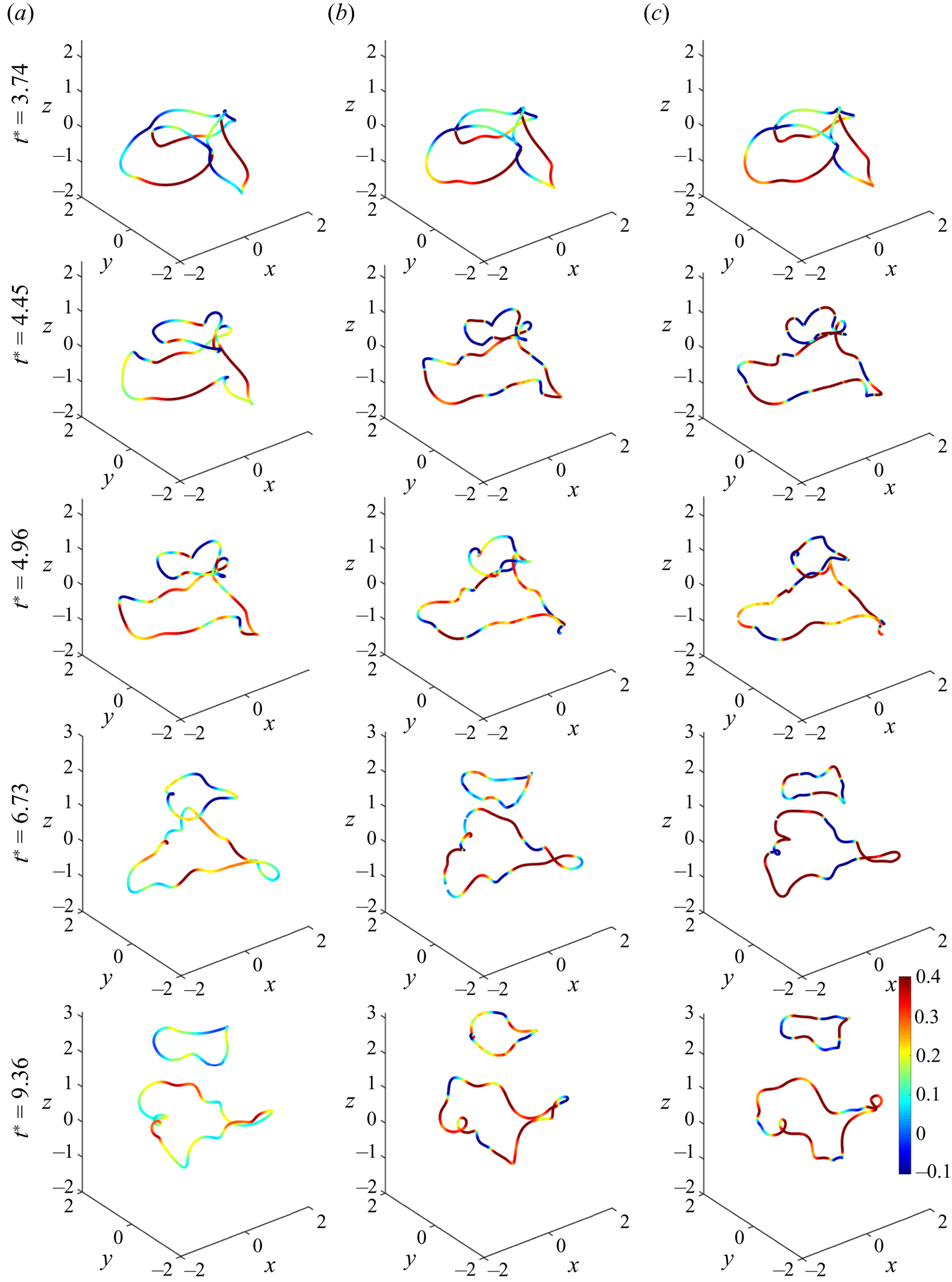
Before going into the details of vortical structures, we first examine the evolution of the vortex core centreline (axis). Note that as vortex lines typically do not align along the vortex core (Schoppa & Hussain Reference Schoppa and Hussain2002; Yao & Hussain Reference Yao and Hussain2018), they cannot be employed to represent the vortex core centreline. How to identify the vortex core axis is still an open question, and numerous approaches have been proposed (Sujudi & Haimes Reference Sujudi and Haimes1995; Tian et al. Reference Tian, Gao, Dong and Liu2018). Here, we use the method developed by Levy, Degani & Seginer (Reference Levy, Degani and Seginer1990) based on the normalized helicity density  $\boldsymbol {u}\boldsymbol {\cdot }\boldsymbol {\omega }/(|\boldsymbol {u}|\,|\boldsymbol {\omega }|)$ and implemented in Paraview by Sadlo et al. (Reference Sadlo, Hausner, Hofmann, Jung, Karch, Peikert, Pilz, Roth and Sdeo2019). The use of normalized helicity density is based on the argument that the angle between the velocity and vorticity vectors is typically minimal near the vortex core axis. It can filter out the regions of low vorticity, as well as regions of high vorticity but low velocity, particularly where the angle between the velocity and vorticity vectors is large. This method works very well in extracting the vortex centrelines, except for the short period when reconnection occurs and the vortex core is non-unique. Figure 5 shows the corresponding centrelines of the structures shown in figure 4, which represent well the vortex knot before reconnection, and SLR and LTR after reconnection. Furthermore, Kelvin waves are observed after reconnection, and the nonlinear interaction among them creates waves of shorter and shorter wavelengths – one of the main mechanisms for energy cascade in quantum reconnection (Baggaley & Barenghi Reference Baggaley and Barenghi2011; Fonda et al. Reference Fonda, Meichle, Ouellette, Hormoz and Lathrop2014).
Evolution of extracted vortex centreline (shaded with centreline helicity density  $h_c=\boldsymbol {u}\boldsymbol {\cdot }\boldsymbol {T}$) for structures shown in figure 4: (a)
 $Re=2000$, (b)
 $6000$ and (c)
 $12\,000$.

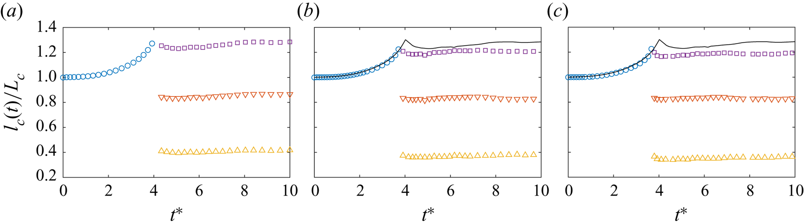
Based on the tracked vortex centrelines, several interesting quantities can be measured. The first one is the length of the vortex centreline  $l_c$. From the local induction approximation of the Biot–Savart model, the total length
 $l_c$ of the vortex is proportional to the kinetic energy
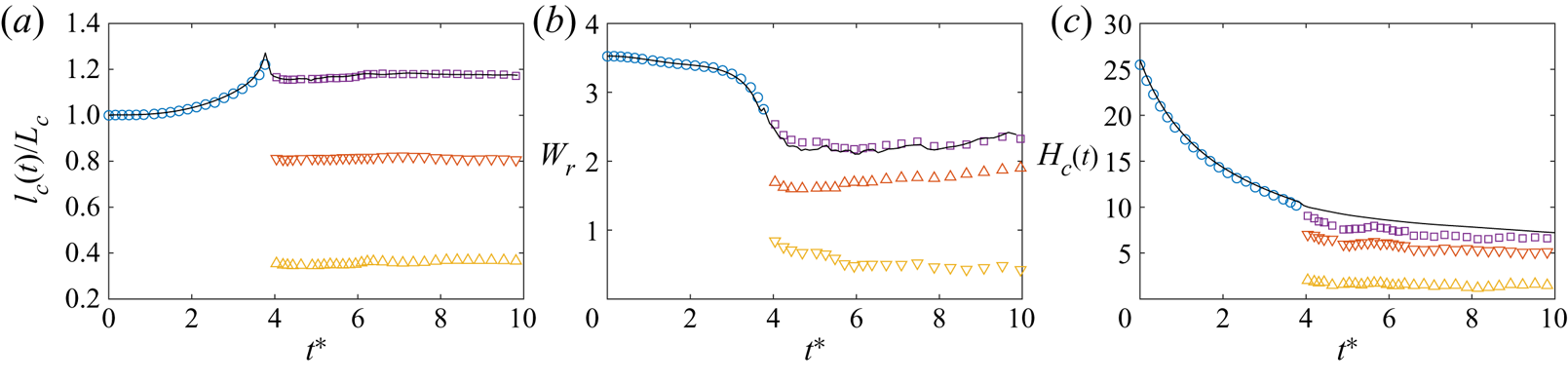
 $E(t)$ (Alamri, Youd & Barenghi Reference Alamri, Youd and Barenghi2008). As energy is ‘dissipated’ as sound radiation during reconnection, a decrease in the total length has been observed from quantum reconnection (Proment & Krstulovic Reference Proment and Krstulovic2020). Figure 6 shows the evolution of lengths for the vortex knot before reconnection and SLR and LTR and their sum after reconnection. Consistent with that observed in Scheeler et al. (Reference Scheeler, Kleckner, Proment, Kindlmann and Irvine2014) for a quantum trefoil knot, the total length
 $l_c(t)$ continuously increases before reconnection, suddenly drops during reconnection, and remains almost constant after reconnection. In addition, before reconnection
 $l_c(t)$ is almost identical for different
 $Re$, but after reconnection it slightly decreases as
 $Re$ increases. Namely, it is approximately 25 %, 18 % and 15 % longer than its initial length
 $L_c$ for
 $Re=2000$,
 $6000$ and
 $12\,000$, respectively. Both the lengths of the large (
 $l^l_c$) and small (
 $l^s_c$) rings decrease as
 $Re$ increases, and their ratio (
 $l^l_c/l^s_c$) slightly increases with
 $Re$, which corresponds to approximately
 $2.0$,
 $2.21$ and
 $2.29$ for
 $Re=2000$,
 $6000$ and
 $12\,000$, respectively. The shorter in total length
 $l_c$ after reconnection at high
 $Re$ is associated with an earlier reconnection. Besides, it seems that the change in
 $l_c$ during reconnection is qualitatively linked to the total energy loss during reconnection: as the energy dissipation is reduced at high
 $Re$, the drop in total length
 $\Delta l$ is also smaller – akin to that found by Proment & Krstulovic (Reference Proment and Krstulovic2020).
Time evolution of the normalized total length  $l_c/L_c$ for the vortex knot before reconnection (circle), and for SLR (
 $\triangle$), LTR (
 $\triangledown$) and their sum (
 $\square$): (a)
 $Re=2000$, (b)
 $6000$ and (c)
 $12\,000$. Note that the total length for the
 $Re=2000$ case (solid lines) is shown in (b,c) as a reference.

The moment of vorticity for a vortex knot in a fluid at rest at infinity is related to the impulse (Batchelor Reference Batchelor2000)
 \begin{equation} \boldsymbol{I} \equiv \tfrac{1}{2} \iiint_{\mathbb{R}^{3}} \boldsymbol{x} \times \boldsymbol{\omega}( \boldsymbol{x}) \,\mathrm{d} V \approx \tfrac{1}{2} \iiint_{\varOmega} \boldsymbol{x} \times \boldsymbol{\omega}( \boldsymbol{x})\,\mathrm{d} V, \end{equation}
which can be approximated by the integral over the periodic domain for the very thin vortex tubes. As a theoretical estimation for the thin vortex filament, substituting  $\boldsymbol {\omega }\,\mathrm {d} V = \varGamma \,\mathrm {d}\boldsymbol {c}$ to (3.1) yields
 \begin{equation} \boldsymbol{I} =\varGamma \boldsymbol{S}, \end{equation}
where  $\boldsymbol {S}=\oint _c\boldsymbol {c}\times \mathrm {d}\boldsymbol {c}/2$ is the directed area enclosed by the curve (Wu, Ma & Zhou Reference Wu, Ma and Zhou2007). Following (3.2), the trefoil knotted vortex specified based on (2.8) has an initial impulse
 $\boldsymbol {I} = (0, 0, 4.5{\rm \pi} )$, which is very close to the value of
 $(0, 0, 14.16)$ numerically calculated over the periodic domain
 $V$ ((3.1)) for the finite thickness case. Since the impulse is a motion invariant, it can be employed to characterize the evolutionary geometry of vortex knots (Xiong & Yang Reference Xiong and Yang2019).
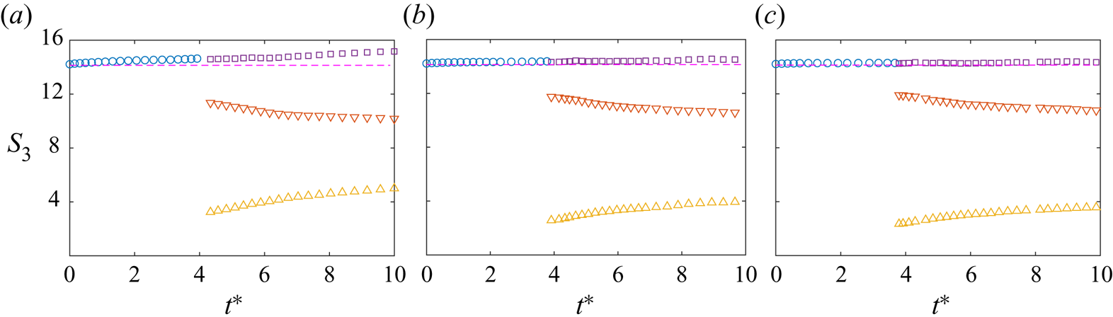
Figure 7 shows the evolution of the third component ( $S_3$) of the directed area enclosed by the vortex centrelines for the vortex knot before reconnection, and for SLR and LTR and their sum after reconnection. Note that the other two components are negligible and, hence, are not shown. For
 $Re=2000$,
 $S_3$ continuously increases with time. As
 $\boldsymbol {I}$ is invariant, the increase of
 $S_3$ is mainly due to the decrease in circulation
 $\varGamma$ through viscous cross-diffusion, which decreases with increasing
 $Re$. Therefore,
 $S_3$ is better conserved at high
 $Re$; and the difference between the calculated value and the theoretical prediction is within
 $1\,\%$ for
 $Re=12\,000$. In addition, due to the mutual induction between SLR and LTR,
 $S_3$ continuously increases and decreases for SLR and LTR, respectively – similar to those observed for the leap-frogging of two co-axial vortex rings (Mariani & Kontis Reference Mariani and Kontis2010; Scheeler et al. Reference Scheeler, van Rees, Kedia, Kleckner and Irvine2017). The rate of change of
 $S_3$ decreases as the two rings separate.
Time evolution of the third components of the directed area enclosed by the vortex centrelines  $S_3$ for the vortex knot before reconnection (circle), and for SLR (
 $\triangle$), LTR (
 $\triangledown$) and their sum (
 $\square$): (a)
 $Re=2000$, (b)
 $6000$ and (c)
 $12\,000$. Note that the dashed lines represent the theoretical value
 $4.5{\rm \pi}$.

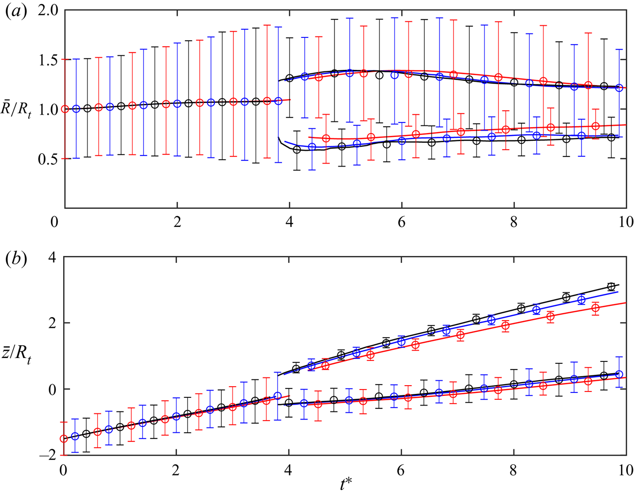
Figure 8 shows the mean radius  $\bar {R}$ and
 $z$-location
 $\bar {z}$ for the vortex knot before reconnection, and for SLR and LTR after reconnection, defined as
 $$\begin{gather} \bar{R}(t)=\frac{1}{L_c}\oint_{C} R(s)\, \textrm{d}s, \end{gather}$$
 $$\begin{gather}\bar{z}(t)=\frac{1}{L_c}\oint_{C} z(s)\, \textrm{d}s. \end{gather}$$
Similar to the total length  $l_c$, the mean radius of the vortex knot
 $\bar {R}$ continuously increases before reconnection and is almost identical among different
 $Re$ cases. The mean radius for the small ring after reconnection
 $\overline {R}^s$ slightly increases with time, which is consistent with the increases of
 $S_3$ (figure 7). In addition, similar to the total length
 $l^s_c$ shown in figure 6,
 $\overline {R}^s$ decreases with increasing
 $Re$. The mean radius of the large ring
 $\overline {R}^l$ slightly increases before it decreases, with the peak occurring earlier as
 $Re$ increases. The difference in the mean radius for the large ring
 $\overline {R}^l$ decreases as
 $Re$ increases and becomes indistinguishable between
 $Re=6000$ and
 $12\,000$ cases.
(a) Mean radius  $\bar {R}$ and (b) mean
 $z$-location
 $\bar {z}$ for the vortex knot before reconnection, and for SLR and LTR for
 $Re=2000$ (red),
 $Re=6000$ (blue) and
 $Re=12\,000\ \textrm {K}$ (black). The bars denote the range between minima and maxima.

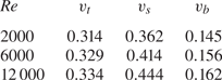
As discussed above, the vortex knot continuously propagates upward during the interaction. Similar to the mean radius, the mean  $z$-location mainly differs for the small ring after reconnection. The propagation velocities for the vortex knot before reconnection, and for SLR and LTR, obtained from linear fitting, are shown in table 1. In general, as
 $Re$ increases, the vortex core size is smaller due to reduced diffusion; hence, the propagation velocities also increase (Dyson Reference Dyson1893). The propagation velocity for the small ring increases significantly, which is partially due to a reduced mean radius as shown in figure 8(a).
Fitted values of the propagation velocity for the vortex knot before reconnection ( $v_t$) and SLR (
 $v_s$) and LTR (
 $v_b$) after reconnection.

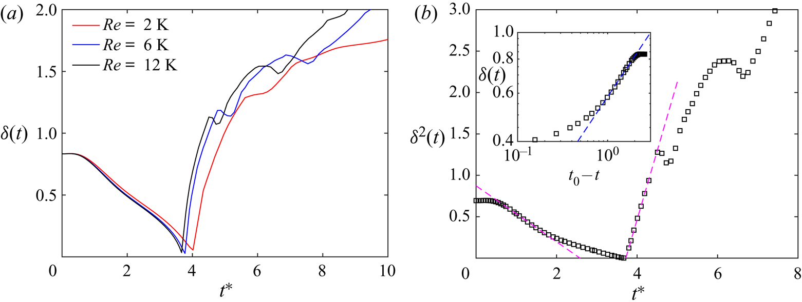
Another interesting question is the separation distances  $\delta (t)$ before and after reconnection (Zuccher et al. Reference Zuccher, Caliari, Baggaley and Barenghi2012). Based on the assumption that reconnection is a localized event and the circulation
 $\varGamma$ is the only relevant dimensional quantity involved, we have
 \begin{equation} \delta(t)=A^{{\pm}}(\varGamma |t-t_0|)^{1/2}, \end{equation}
where  $t_0$ is the reconnection time, and
 $A^{-}$ and
 $A^{+}$ are dimensionless factors for pre- and post-reconnection, respectively. This scaling follows dimensional analysis and has been observed for reconnection of line vortices (Kimura & Moffatt Reference Kimura and Moffatt2017) and also for reconnection of quantized vortices (Fonda et al. Reference Fonda, Meichle, Ouellette, Hormoz and Lathrop2014; Villois, Proment & Krstulovic Reference Villois, Proment and Krstulovic2017). Our recent results on thin core vortices show that such 1/2-power scaling is also valid for classical viscous reconnection (Yao & Hussain Reference Yao and Hussain2020a,Reference Yao and Hussainc).
Figure 9(a) displays the evolution of  $\delta (t)$ for vortex knot before reconnection and between SLR and LTR after reconnection, with (b–d) showing the corresponding
 $\delta ^2(t)$. During the initial phase of forming anti-parallel configuration,
 $\delta (t)$ slowly varies. Then, it rapidly decreases as the perturbed vortex tubes approach each other due to self-induction. A slight difference in the evolution of
 $\delta (t)$ can be observed among different
 $Re$ cases, indicating a weak
 $Re$ effect on the pre-reconnection evolution. In general,
 $\delta (t)$ decreases more rapidly as
 $Re$ increases, which is mainly due to a high self-induced velocity associated with a smaller vortex core size and radius of curvature (Yao & Hussain Reference Yao and Hussain2020a). The distinct agreement with linear scaling for
 $\delta ^2(t)$ at the early time suggests that
 $\delta (t)\sim a^{-} (t^-_0-t)^{1/2}$, with
 $a^{-}$ the constant prefactors for pre-reconnection corresponding to
 $A^-\varGamma ^{1/2}$ in (3.5), and
 $t^-_0$ the critical time when
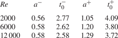
 $\delta \to 0$. The values of
 $a^{-}$ and
 $t^-_0$ for different
 $Re$ obtained from linear fitting on
 $\delta ^2(t)$ during
 $0.5< t<2$ are listed in table 2. As the circulation remains almost constant at
 $\varGamma =1$ during this phase, the dimensionless prefactor
 $A^{-}\approx a^{-}$ and is quite close to that reported in Villois et al. (Reference Villois, Proment and Krstulovic2017) for a quantized trefoil vortex knot. Note that
 $\delta ^2(t)$ slowly deviates from linear scaling when
 $\delta \sim {O}(\sigma )$. The deviation happens earlier at small
 $Re$ – due to the more rapid increase of the core size caused by higher viscous diffusion.
Time evolutions of (a) separation distance  $\delta (t)$ and (b)
 $\delta ^2(t)$ for
 $12\,000$. In panel (b) the dashed lines indicate linear scaling for pre- and post-reconnection, and the inset is
 $\delta$ as a function of
 $|t -t_0|$ for pre-reconnection.

Fitted values of the prefactors  $a^{\pm }$ and
 $t^{\pm }_0$ for the minimum distance scaling
 $\delta (t)\sim a^{\pm }|t-t^\pm _0|^{1/2}$. The superscript
 $\pm$ stands for before (
 $-$) and after (
 $+$) the reconnection, respectively.

After reconnection, a clear linear scaling for  $\delta ^2(t)$ can be observed (figure 9b–d). Hence,
 $\delta \sim a^{+}(t-t^{+}_0)^{1/2}$ scaling also holds in the post-reconnection phase. A fit in the linear region gives
 $t^+_0\approx 4.09$,
 $3.80$ and
 $3.72$, and
 $a^+=1.05$,
 $1.20$ and
 $1.29$ for
 $Re=2000$,
 $6000$ and
 $12\,000$, respectively. Consistent with previous studies (Villois et al. Reference Villois, Proment and Krstulovic2017),
 $a^+$ is always larger than
 $a^-$, indicating that the vortices separate much faster than when they approach each other. Compared with the pre-reconnection phase, the
 $Re$ effect on
 $\delta (t)$ is more apparent during the post-reconnection. It is because, in classical fluids, the dynamics of reconnection, such as the reconnection time and the circulation transfer rate, strongly depends on viscosity
 $\nu$. Reconnection is typically faster and more complete at higher
 $Re$ (Hussain & Duraisamy Reference Hussain and Duraisamy2011; Yao & Hussain Reference Yao and Hussain2020a). When the two vortex rings move sufficiently far apart, the
 $1/2$ scaling breaks down, and the deviation from
 $1/2$ occurs earlier for higher
 $Re$ – due to stronger Kelvin waves. Note that although, on average, the two vortex rings travel almost at a constant speed, the crossover between the
 $t^{1/2}$ to
 $t^1$ scalings for
 $\delta (t)$ suggested by Galantucci et al. (Reference Galantucci, Baggaley, Parker and Barenghi2019) is not observed here. It is mainly because, due to the strong variation of local curvature, each segment of the vortex ring travels at a different speed – evident from the large variation in the
 $z$-location, particularly for LTR (figure 8b).
4. Helicity dynamics
4.1. Centreline helicity, Writhe, torsion and self-link number
For sufficiently thin vortex tubes with minimal vorticity variation across the cross-section, the total helicity is encoded completely in the flow along the centreline of the vortex tube (Bretherton Reference Bretherton1970; Scheeler et al. Reference Scheeler, van Rees, Kedia, Kleckner and Irvine2017); hence,
 \begin{equation} H_c=\sum_i \varGamma_i \oint_{C_i} \boldsymbol{u}(s)\boldsymbol{\cdot}\boldsymbol{T}(s) \,\textrm{d}s, \end{equation}
where  $h_c=\boldsymbol {u}\boldsymbol {\cdot }\boldsymbol {T}$ is the centreline helicity density and
 $\boldsymbol {T}$ again denotes the unit tangential vector along the vortex centreline
 $C$. The centreline helicity
 $H_c$ is sometimes used to represent the writhe helicity, which is based on the assumption that the twist helicity is dissipated rather rapidly, particularly for a very thin vortex (Scheeler et al. Reference Scheeler, Kleckner, Proment, Kindlmann and Irvine2014).
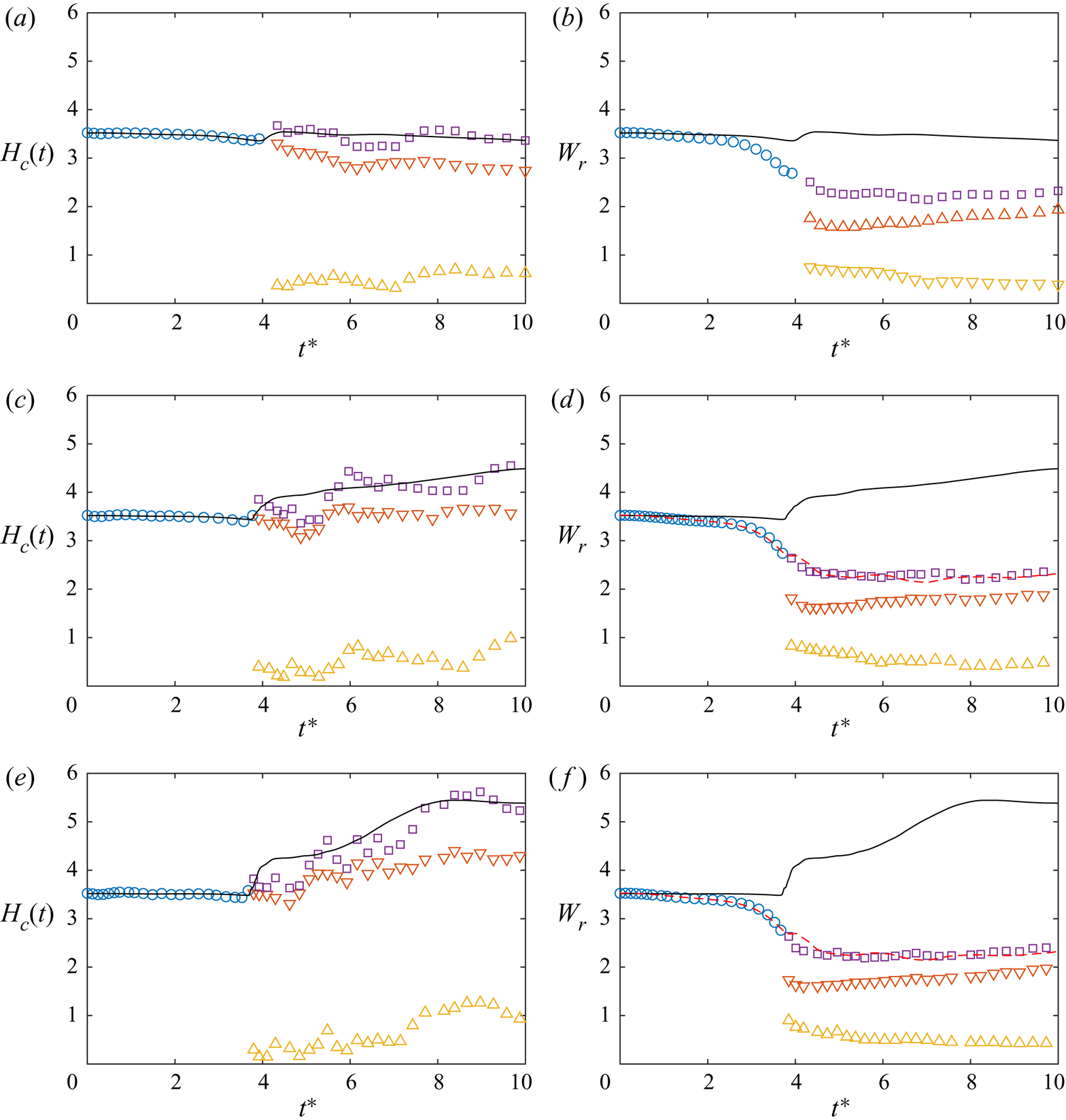
Figure 10(a,c,e) show centreline helicity  $H_c$ for the vortex knot before reconnection and for SLR and LTR and their sum after reconnection. In addition, the global helicity
 $H$ and the helicity for SLR and LTR (
 $H^s=\int _{V^s} h\,\mathrm {d}V^s$ and
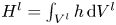 $H^l=\int _{V^l} h\,\mathrm {d}V^l$ with
 $V^s$ and
 $V^l$ denoting the volume occupied by SLR and LTR) are also included for comparison. Note that when calculating
 $H_c$, we assume the circulation remains the same as the initial value
 $\varGamma$. Due to limited viscous cross-diffusion, particularly at high
 $Re$, this assumption should be valid before reconnection. As reconnection in viscous flows is not complete, the circulations of the bridges in the SLR and LTR are smaller than
 $\varGamma$ after reconnection – due to the presence of the remnant threads. However, compared with other unreconnected parts in SLR and LTR, where the circulation remains unchanged as
 $\varGamma$, the bridge is rather short. Hence, on the average, it should still be acceptable to assume that the SLR and LTR have constant circulation
 $\varGamma$ after reconnection. The constant circulation assumption is also employed for calculating writhe helicity
 $\varGamma ^2W_r$. It can be seen that
 $H_c$ is almost identical to
 $H$ for the vortex knot before reconnection – confirming that
 $H_c$ is a reasonably good approximation for
 $H$.
Time evolutions of (a,c,e) the centreline helicity  $H_c$ and (b,d,f) the writhe
 $W_r$ for the vortex knot before reconnection (circle), and for SLR (
 $\triangle$), LTR (
 $\triangledown$) and their sum (
 $\square$): (a,b)
 $Re=2000$, (c,d)
 $6000$ and (e,f)
 $12\,000$. Note that the black solid lines represent the global helicity
 $H$, and the black dashed and dash–dotted lines in (a,c,e) represent the total helicity for LTR and SLR, respectively, and the red dashed lines in (d,f) denote
 $W_r$ for
 $Re=2000$.

After reconnection,  $H_c$ experiences oscillations, which indicates that the axial flows along the vortex rings grow and annihilate. In addition,
 $H_c$ deviates from
 $H$, presumably for two main reasons. First, reconnection causes strong core deformation near the interaction region, such as forming vortex sheets; as a result, the vortex core becomes irregular with a strong vorticity variation. Second, as shown in figure 4, the threads, which are polarized, also contain a significant amount of helicity density which is excluded by
 $H_c$. As expected, the deviation between
 $H_c$ and
 $H$ becomes severe as
 $Re$ increases. Nevertheless,
 $H_c$ can successfully capture the trend of
 $H$ for both rings. For SLR,
 $H_c$ (and also
 $H^s$) always grows with time, and the rate of growth increases with
 $Re$. For
 $Re=2000$,
 $H_c$ (and
 $H^l$) for LTR is found to decrease with time; however, at
 $Re=12\,000$, it reverses and slightly increases at late time. Due to viscous damping,
 $H_c$ becomes less oscillated at late time. Besides, as the vortex core of the two rings becomes regular (i.e. circular) and threads become weaker due to viscous diffusion,
 $H_c$ eventually agrees with
 $H$ again. Note that the increase in
 $H_c$ after reconnection is different from the constant
 $H_c$ observed in the experiment by Scheeler et al. (Reference Scheeler, Kleckner, Proment, Kindlmann and Irvine2014), presumably for two main reasons. First, as shown in figure 5, strong oscillations appear in axial velocity along the vortex tubes. There might be some inaccuracy for measuring the centreline helicity density
 $h_c$ in the experiment. Second, different from three simultaneously reconnections for the ideal trefoil vortex knot considered here, there is only one reconnection at a time in the experiment, as the vortex knot is perturbed. Hence, the increase of
 $H_c$ in the experiment may not be so distinct and sharp.
Figure 10(b,d,f) show the writhe  $W_r$ calculated using (2.3) for the vortex knot before reconnection, as well as for SLR, LTR and their sum after reconnection. As the numerical computation of writhe is very sensitive to small-scale noise in the extracted centreline, a local smoothing filter similar to that used in Scheeler et al. (Reference Scheeler, Kleckner, Proment, Kindlmann and Irvine2014) is applied to the raw data (only for the small and large rings after reconnection). Before reconnection,
 $W_r$ continues to decrease, and after reconnection it has a big drop (but still remains continuous) during the reconnection. Note that the behaviour of
 $W_r$ here is similar to that observed for reconnections in superfluids (Scheeler et al. Reference Scheeler, Kleckner, Proment, Kindlmann and Irvine2014; Proment & Krstulovic Reference Proment and Krstulovic2020). We note with interest that Laing et al. (Reference Laing, Ricca and Sumners2015) proved that
 $W_r$ should be conserved during reconnection of two ideal anti-parallel vortex segments. After reconnection, SLR and LTR are being stretched and compressed, respectively. As a consequence,
 $W_r$ continuously increases/decreases for the SLR/LTR, but their sum remains roughly constant. It is interesting to observe that
 $W_r$ seems to be
 $Re$ independent, and the total drop of
 $W_r$ is
 $\Delta W_r \sim 1\varGamma ^2$. Scheeler et al. (Reference Scheeler, Kleckner, Proment, Kindlmann and Irvine2014) found that
 $\Delta W_r$ strongly depends on the geometry of the trefoil knot, such as the radius to core size ratio
 $R_t/r_e$. Note that from figure 10, it is also clear that
 $H_c$ can not be employed to approximate the writhe helicity
 $\varGamma ^2W_r$, because the assumption that the twist helicity is dissipated rather rapidly in a thin vortex is no longer valid during viscous reconnection – to be discussed in detail later.
Dramatic helicity change is typically associated with topological changes, but we observe a gradual change in both global and writhe helicities (even when reconnections are not taking place). Because the centreline topology is not altered before reconnection, the major writhe-helicity changes should be attributed to geometric deformations of the vortex – coiling or uncoiling. As suggested by Scheeler et al. (Reference Scheeler, van Rees, Kedia, Kleckner and Irvine2017), during vortex evolution, helicity can transfer between writhe and twist; for example, writhe is increased through coiling or decreased through straightening. This helicity conversion mechanism can explain the writhe evolution observed here. Before reconnection  $W_r$ decays faster than the global helicity. This is because, as initially the vortex knot undergoes stretching, part of the writhe helicity is converted to twist helicity. After reconnection, when the two vortex rings form, SLR is stretched by the LTR, hence, its writhe helicity is continuously transferred into twist helicity. On the other hand, as LTR is under compression, its
 $W_R$ slightly increases. In addition, this conversion mechanism is inviscid, which explains why the evolution of writhe is almost
 $Re$ independent.
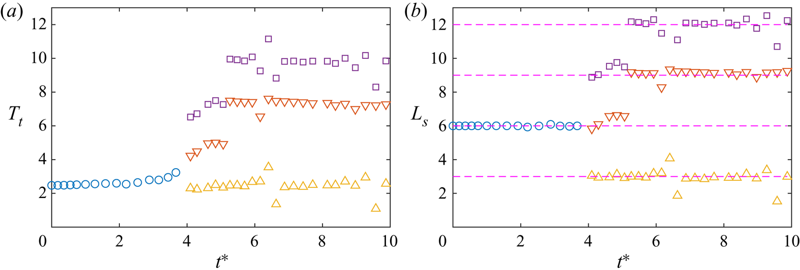
Figure 11 further shows the torsion  $T_t$ (2.5) and self-linking number
 $L_s\equiv W_r+T_s$ for the vortex knot before reconnection, and also for SLR and LTR at
 $Re=12\,000$. (Note that the results for
 $Re=2 000$ and
 $6 000$ are quite similar and, hence, are not shown for brevity.) Before reconnection
 $T_t$ continues to increase and
 $L_s$ remains constant. A similar conservation of
 $L_s$ has also been reported by Kerr (Reference Kerr2018b) for the evolution of coiled vortex rings. To avoid confusion, note that
 $T_t$ is equivalent to ‘
 $T_w$’ defined in Kerr (Reference Kerr2018b, Reference Kerrc). During reconnection, when the vortex knot undergoes dramatic changes in topology,
 $T_t$ and
 $L_s$ also change abruptly, which is different from the torsion conservation for the ideal anti-parallel reconnecting segments in Laing et al. (Reference Laing, Ricca and Sumners2015). Note that the integer
 $L_s$ jumps discontinuously through
 ${\pm }1$ as a curve passes through a configuration containing a point of inflexion (Moffatt & Ricca Reference Moffatt and Ricca1992). Due to the presence of three additional inflexion points, the initial
 $L_s$ for our configuration is
 $6$, which is larger than those employed by Scheeler et al. (Reference Scheeler, Kleckner, Proment, Kindlmann and Irvine2014) and Yu et al. (Reference Yu, Chapelier and Scalo2018) (i.e.
 $L_s=3$). Owing to the tri-symmetry of the trefoil knot, the curve deformation during the reconnection involves passage through three inflexional configurations, and self-linking numbers for the two unlinked rings become
 $L_s = 6 \pm 3$. After reconnection,
 $T_t$ for the small/large rings slightly increases/decreases with time, and
 $L_s$ for the small and large rings remains almost constant at
 $3$ and
 $9$, respectively. Moreover, the numerical calculation of
 $T_t$ is very sensitive at the inflexional configuration for which
 $T_t$ is discontinuous by
 ${\pm }1$; so
 $T_t$ and
 $L_k$ have some notable oscillations in figure 11.
Time evolution of (a) the torsion  $T_t$ and (b) the self-link number
 $L_s$ for the vortex knot before reconnection (circle), and for SLR (
 $\triangle$), LTR (
 $\triangledown$) and their sum (
 $\square$) at
 $Re=12\,000$.

4.2. Transient helicity growth
An important question is why global helicity  $H$ increases after reconnection for high
 $Re$ cases. The governing equation for the helicity density
 $h$ is
 \begin{equation} \frac{\mathrm{D} h}{\mathrm{D}t}=\underbrace{-\boldsymbol{\omega}\boldsymbol{\cdot}\boldsymbol{\nabla}(p/\rho-\boldsymbol{u}^2/2)}_{production}+\underbrace{\nu\nabla^2h}_{diffusion}-\underbrace{2\nu\boldsymbol{\omega} \boldsymbol{\cdot}(\boldsymbol{\nabla} \times \boldsymbol{\omega})}_{dissipation}, \end{equation}
where the terms on the right-hand side are the helicity production, diffusion and dissipation, respectively (Kerr Reference Kerr2018a);  $\boldsymbol {\omega } \boldsymbol {\cdot }(\boldsymbol {\nabla } \times \boldsymbol {\omega })$ is the so-called ‘superhelicity’ (Brissaud et al. Reference Brissaud, Frisch, Leorat, Lesieur and Mazure1973; Hide Reference Hide1989; Scheeler et al. Reference Scheeler, Kleckner, Proment, Kindlmann and Irvine2014). Note that both helicity production and diffusion terms vanish when integrated over the periodic computational domain. Therefore, the variation of
 $H$ is purely due to viscous dissipation
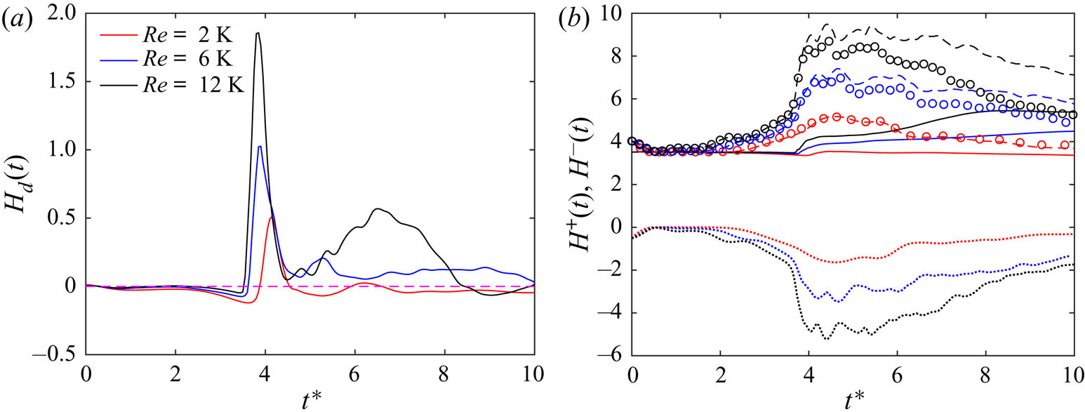
 $H_d=-2\nu \int _V \boldsymbol {\omega } \boldsymbol {\cdot }(\boldsymbol {\nabla } \times \boldsymbol {\omega }) \,\mathrm {d}V$. As
 $H$ is not positive-sign definite,
 $H_d$ – different from energy or enstrophy dissipation – can be either positive or negative. However, as shown later in figure 13(d–f), the helicity dissipation density
 $h_d$ (
 $=-2\nu \boldsymbol {\omega } \boldsymbol {\cdot }(\boldsymbol {\nabla } \times \boldsymbol {\omega })$) is typically negative where
 $h$ is positive, and vice versa.
Figure 12(a) shows the time evolution of volume integration of  $H_d$ for different
 $Re$. Note that negative/positive values of
 $H_d$ denote decreases/increases of
 $H$, respectively. Before reconnection (
 $t^*<3.5$),
 $H$ is transferred from writhe to twist helicity, which then decays due to dissipation; thus,
 $H_d$ is slightly negative. During reconnection,
 $H_d$ surges, and its rate of growth increases with
 $Re$. The time of the peak of
 $H_d$ to occur decreases as
 $Re$ increases, which is consistent with the earlier reconnection at higher
 $Re$. After reconnection,
 $H_d$ becomes negative again for
 $Re=2000$ but remains positive for the two high
 $Re$ cases, which agrees with the increases of
 $H$. Interestingly, there is a distinct second peak around
 $t^*=6.5$ for
 $Re=12\,000$ – yet to be explained.
Time evolution of (a) helicity dissipation  $H_d$ and (b)
 $H^{\pm }$ for
 $Re=2000$ (red),
 $6000$ (blue) and
 $12\,000$ (black). Note that the circles in (b) denote
 $-H^-(t)+H(0)$, with
 $H(0)=3.52$ the initial global helicity.

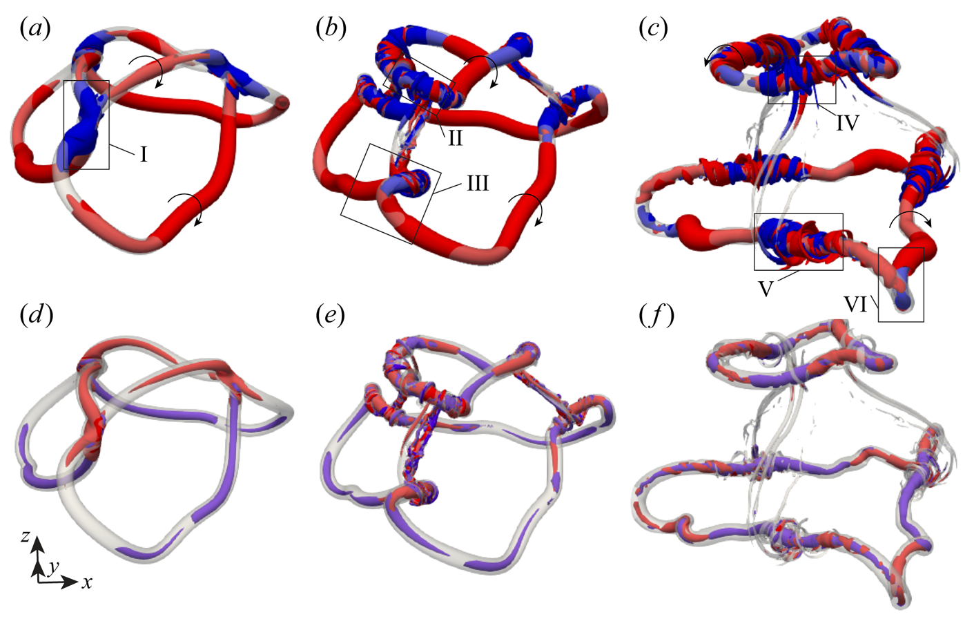
Figure 13(a–c) show the distribution of helicity density at several instants for  $Re=6000$ with figure 13(d–f) showing the corresponding helicity dissipation density
 $h_d$. Again, different from energy or enstrophy, helicity is not positive-sign definite. Hence, in the positive
 $h$ region, negative
 $h_d$ indicates helicity dissipation, while in the negative
 $h$ region, positive
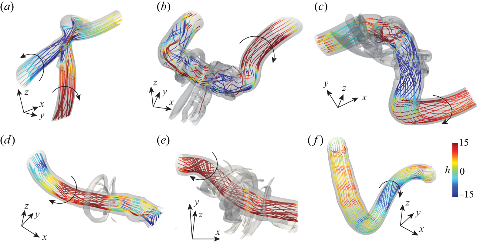
 $h_d$ suggests helicity dissipation. First, as the knotted vortex propagates upward (along the
 $z$-direction), structures with negative helicity density appear in the reconnection region – suggesting that the anti-parallel structures are oppositely polarized (see figure 14(a) for a better view). As a consequence, the bridges formed during reconnection also become oppositely polarized between two legs (figure 14b,c), similar to that sketched by Melander & Hussain (Reference Melander and Hussain1988) and Kida & Takaoka (Reference Kida and Takaoka1994) and observed by van Rees, Hussain & Koumoutsakos (Reference van Rees, Hussain and Koumoutsakos2012) for reconnection of anti-parallel vortex tubes. However, there is one important difference: for the anti-parallel cases considered by Melander & Hussain (Reference Melander and Hussain1988) and others, reconnection is exactly symmetric, and the helicity density in the two legs have equal strengths; however, reconnection here is asymmetric, and, as we will show later, the helicity density in the two legs have unequal strengths. The negative helicity density dominates the positive for the bridge in SLR, while it reverses for the bridge in LTR. At late times (e.g.
 $t^*=6.01$), negative
 $h$ regions are mainly located in the threads that wrap around the rings (region IV–V in figure 13c) and the kinked part of the rings (region VI in figure 13c). Figure 13(d–f) show that the regions with strong
 $h$ have strong
 $h_d$ of opposite sign – indicating that large helicity dissipation occurs in strong helical region. However, it is rather difficult to tell from figure 13(d–f) whether the total dissipation
 $H_d$ is positive or negative.
Isosurface of (a–c) helicity density  $h=\boldsymbol {u}\boldsymbol {\cdot } \boldsymbol {\omega }$ and (d–f) helicity dissipation
 $h_d=-2\nu \boldsymbol {\omega } \boldsymbol {\cdot }(\boldsymbol {\nabla } \times \boldsymbol {\omega })$ for
 $Re=6000$ at: (a,d)
 $t^*=3.74$, (b,e)
 $t^*=4.29$ and (c,f)
 $t^*=6.01$. Note that the red and blue colours denote positive and negative of
 $5\,\%$ of the maximum value, and the transparent (grey) isosurface represents
 $|\boldsymbol {\omega }|=0.04\omega _0$. The black arrows indicate the direction of vortex rotation.

Vortex lines shaded with helicity density for structures I–VI marked in figure 13. The black arrow indicates the rotating direction of the vortex.

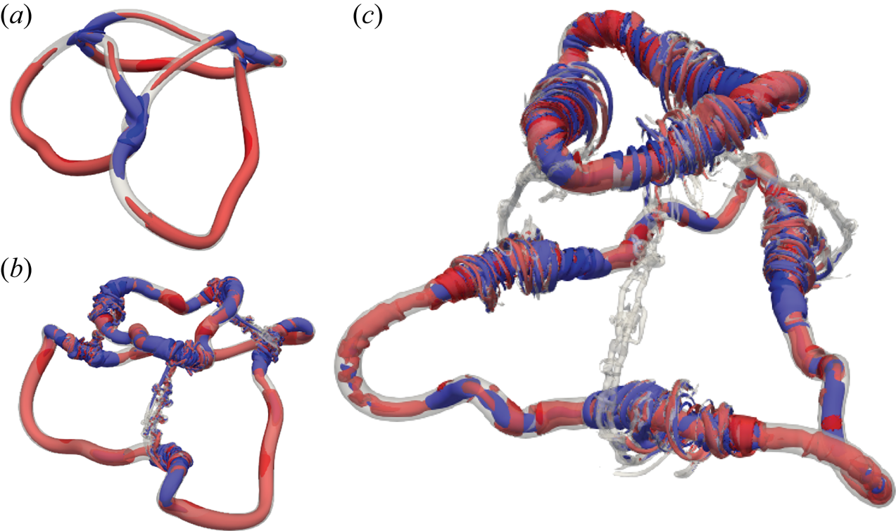
Figure 15 shows the isosurface of helicity density for  $Re=12\,000$. Due to reduced viscous diffusion, the structures look thinner than those at
 $Re=6000$ (figure 13). Similar to that at
 $Re=6000$, initially the negative
 $h$ structures are mainly located in the anti-parallel reconnection region (figure 15a). Compared with that at
 $Re=6000$, more negative
 $h$ structures are observed after reconnection, especially in SLR (figures 15b). At a late time, these structures cascade into smaller scales. Besides, the rings are wrapped around with numerous threads, which are polarized due to flow induced by the rings – akin to that observed in vortex-turbulent interaction (Pradeep & Hussain Reference Pradeep and Hussain2010). In addition, the threads that connect SLR and LTR further undergo reconnection forming secondary bridges, similar to that observed in Yao & Hussain (Reference Yao and Hussain2020b). However, compared with elsewhere,
 $h$ there is negligible due to rapid dissipation caused by a rather small core size.
Isosurface of helicity density  $h=\boldsymbol {u}\boldsymbol {\cdot } \boldsymbol {\omega }$ for
 $Re=12\,000$ at: (a)
 $t^*=3.63$, (b)
 $t^*=4.29$ and (c)
 $t^*=6.01$. Note that the red and blue colours denote positive and negative
 $5\,\%$ of the maximum value, and the transparent (grey) isosurface represents
 $|\boldsymbol {\omega }|=0.04\omega _0$.

Although the global helicity is positive, as shown in figures 13 and 15, structures with strong negative  $h$ evolve during reconnection. In addition, the negative
 $h$ structures increase with
 $Re$ and can survive for a very long time after reconnection. To quantify that, figure 12(b) further shows the volume-integrated positive and negative helicity
 $H^{\pm }=\int h^{\pm } \,\mathrm {d}V$, where
 \begin{equation} h^+{=} \begin{cases} h, & \text{if } h\geq 0,\\ 0, & \text{otherwise}, \end{cases} \end{equation}
and  $h^-=h-h^+$. Note that a small non-zero value of
 $H^-$ exists at an early time, presumably due to our specific initial condition (i.e. the three ‘kinks’ in the inner circle). As it rapidly decreases to zero due to viscous dissipation, it has a negligible effect on late evolution. It is interesting to observe that both
 $H^-$ and
 $H^+$ slowly grow during the initial stage when the knotted vortex starts to form anti-parallel structures. Just before reconnection, both of them rapidly increase at roughly the same rate; hence,
 $H$ remains roughly conserved. This is somehow expected, as the helicity production
 $H_p$ should produce zero net helicity ((4.2)). Consistent with
 $H$, the growth rate of
 $H^\pm$ increases with
 $Re$. After reconnection, the magnitudes of both
 $H^+$ and
 $H^-$ decrease, but non-monotonically. Surprisingly, at high
 $Re$, the decay rate for
 $H^-$ is found to be larger than
 $H^+$. It implies that generation of twisted structures and the more rapid decay of those with negative
 $h$ cause the net growth of
 $H$ for
 $Re=6000$ and
 $12\,000$.
4.3. Mechanism for transient helicity growth
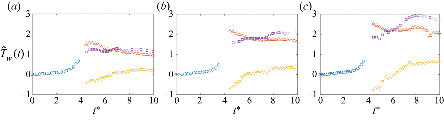
Figure 16 shows the evolution of  $\tilde {T}_w$ for the vortex knot before reconnection and for SLR and LTR and their sum after reconnection. Several comments deserve to be made. First,
 $\tilde {T}_w$ is equal to
 $T_w$ at
 $t^*=0$, or even before reconnection occurs. During and after reconnection, due to the presence of linked vortex lines, such as those in the threads, which connect two rings, and those in localized linked structures (figure 15),
 $\tilde {T}_w$, which also has some contributions from
 $L_k$, is no longer equivalent to
 $T_w$. As shown in figure 11, the increase of
 $\tilde {T}_w$ (and also
 $T_w$) before reconnection is mainly due to the growth of torsion
 $T_t$ converted from writhe
 $W_r$. Note that although the net contribution of intrinsic twist
 $T_i$ to
 $\tilde {T}_w$ is small, it does not mean that it is small everywhere. Instead, as discussed in Yao & Hussain (Reference Yao and Hussain2021), the intrinsic twist helicity is mainly generated through an inviscid splitting mechanism, where structures with positive and negative intrinsic twist are generated simultaneously and equally (figures 13 and 15).
Time evolution of the generalized twist  $\tilde {T}_w$ (calculated as
 $H/\varGamma ^2-W_r$) for the vortex knot before reconnection (circle), and for SLR (
 $\triangle$), LTR (
 $\triangledown$) and their sum (
 $\square$): (a)
 $Re=2000$, (b)
 $6000$ and (c)
 $12\,000$.

After reconnection, the total generalized twist  $\tilde {T}_w$ slightly decreases for
 $Re=2000$ but increases for the two high
 $Re$ cases – consistent with the variation of the global helicity
 $H$ (figure 3b). Since after reconnection the trefoil knot develops into two separate coiled vortex rings, their dynamics and interaction should explain the post-reconnection evolution of
 $\tilde {T}_w$ and
 $H$. In addition, the increase of total
 $\tilde {T}_w$, as well as
 $H$ for high
 $Re$ after reconnection is mainly due to the increase of
 $\tilde {T}_w$ in SLR. We find that just after reconnection, the LTR is overall positively twisted, while SLR is predominantly negatively twisted. It suggests that the newly generated helicity density
 $h$ is unequally divided into small and large rings, with more negative
 $h$ being transferred into the small ring. This unequal splitting of
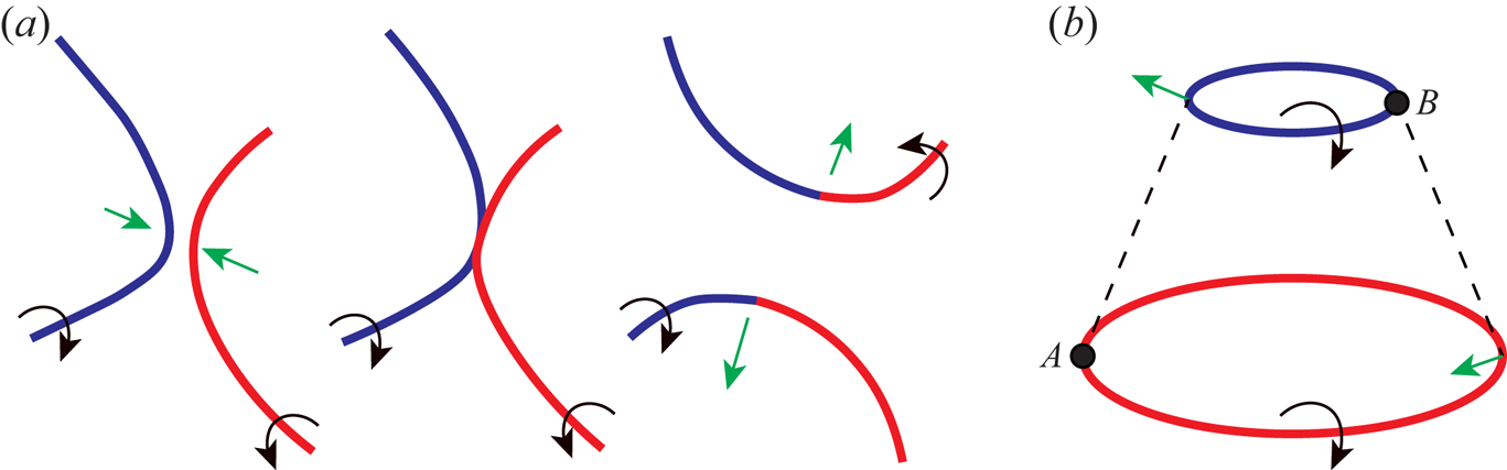
 $h$ is again mainly due to asymmetric reconnection, which is further illustrated in figure 17(a). Two vortex filaments with opposite signs of
 $h$ collide and reconnect asymmetrically to form two new filaments, with one associated with predominant positive
 $h$ and the other with negative
 $h$.
Schematic of (a) asymmetric reconnection of two vortex filaments with opposite sign of helicity density, and (b) mutual induction between two co-axial vortex rings. The black arrows denote the rotating direction of the vortex filaments, and the green arrows represent the induced velocity.

For the negatively twisted SLR,  $\tilde {T}_w$ slowly decays due to viscous dissipation, causing the total helicity for SLR to increase (figure 10a). As
 $Re$ increases, more negative
 $h$ are generated before and during reconnection (figure 12b). Consequently, negative twist in SLR is enhanced after reconnection, which results in an increased dissipation of twist helicity, hence a rapid growth of
 $\tilde {T}_w$ – despite the fact that viscosity
 $\nu$ is reduced. Note that different from a single coiled ring (Scheeler et al. Reference Scheeler, Kleckner, Proment, Kindlmann and Irvine2014), where
 $\tilde {T}_w$ eventually decays to zero, here
 $\tilde {T}_w$ of SLR alternate in sign and becomes positive at late time. The reason is that as SLR is stretched, part of the writhe helicity is converted to the twist helicity, similar to that happening to the trefoil knot before reconnection. A LTR is initially associated with a positive net twist, which then continuously decreases due to viscous dissipation. Note that different from SLR, the decay rate of LTR decreases with
 $Re$, with is mainly attributed to smaller
 $\nu$.
From figure 16, the different behaviours of twist and global helicity evolution at different  $Re$ are mainly due to differing twist decay rates for SLR and LTR. For a twisted rectilinear vortex column, the relative dissipation of twist depends mainly on core size
 $\sigma$ and viscosity
 $\nu$, i.e.
 $\partial T_w/\partial t=-2\nu T_w/\sigma ^2$. However, for a coiled vortex ring, due to the presence of writhe and twist conversion, the dissipation may also be affected by its geometry, such as the ratio between core size and radius (
 $\sigma /R$) and the writhe. For example, Scheeler et al. (Reference Scheeler, van Rees, Kedia, Kleckner and Irvine2017) showed that
 $\partial T_w/\partial t$ increases with
 $\sigma /R$ for a three-coiled vortex ring. Furthermore, for the interacting coiled vortex rings considered here, the dissipation also depends on the influence of the other ring. The induced motion of LTR stretches the SLR (figure 17b), causing more rapid energy and helicity cascade to small scales (figures 15c); hence more dissipation. To account for these effects, we simply include a correction term
 $g$ in the twist dissipation, which yields
 \begin{equation} \frac{\partial T_w}{\partial t}={-}cgT_w, \end{equation}
where  $c$ represents
 $2\nu /\sigma ^2$. As the geometries of SLR and LTR vary very mildly with
 $Re$, for simplicity, we further assume
 $g$ is independent of
 $Re$. Accordingly, the twist for each ring follows
 \begin{equation} T_w=T_{w,0}\,\textrm{e}^{{-}cgt}. \end{equation}
From figure 16 we have the following relationship regarding the initial twist in SLR ( $T^s_{w,0})$ and LTR (
 $T^l_{w,0}$):
 \begin{equation} T^s_{w,0}<0,\quad T^l_{w,0}>0,\quad |T^s_{w,0}|<|T^l_{w,0}|. \end{equation}
Therefore, the total twist can be expressed as
 \begin{equation} T_w=|T^l_{w}|-|T^s_{w}|=|T^l_{w,0}|e^{{-}cg^lt}-|T^s_{w,0}|e^{{-}cg^st}. \end{equation}
Using the first-order Taylor expansion, we have
 \begin{align} T_w&=|T^l_{w}|-|T^s_{w}|=|T^l_{w,0}|(1-cg^lt)-|T^s_{w,0}|(1-cg^st)\nonumber\\ &=\Delta T_{w,0}+\left(1-\frac{g^l|T^l_{w,0}|}{g^s|T^s_{w,0}|}\right)cg^s|T^s_{w,0}|t, \end{align}
where  $\Delta T_{w,0}=|T^l_{w,0}|-|T^s_{w,0}|$ is almost
 $Re$ independent. From (4.8), the evolution of
 $T_w$ mainly depends on the ratio between
 $g^l|T^l_{w,0}|$ and
 $g^s|T^s_{w,0}|$. As SLR is associated with a larger
 $\sigma /R$ and is under stretching, it is expected to have
 $g^s>g^l$. At
 $Re=2000$, the initial twist for LTR (
 $|T^l_{w,0}|\approx 1.5$) is much larger than that of SLR (
 $|T^s_{w,0}|\approx 0.5$). As a result,
 $(g^l|T^l_{w,0}|)/(g^s|T^s_{w,0}|)>1$; hence,
 $T_w$ decreases with time. However, the difference between
 $|T^l_{w,0}|$ and
 $|T^s_{w,0}|$ decreases as
 $Re$ increases. In particular,
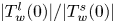 $|T^l_w(0)|/ |T^s_w(0)|$ becomes approximately
 $2$ and
 $5/3$ at
 $Re=6000$ and
 $12\,000$. As a result,
 $(g^l|T^l_{w,0}|)/g^s|T^s_{w,0}|<1$. Furthermore, at very high
 $Re$,
 $|T^l_w(0)|/ |T^s_w(0)| \to 1$, and
 $(g^l|T^l_{w,0}|)/g^s|T^s_{w,0}|$ would approach
 $g^l/g^s$. Hence,
 $T_w$ grows with time at high
 $Re$, and the rate of growth increases with
 $Re$, which is consistent with those observed in figure 16. Note that both
 $T^l_w$ and
 $T^s_w$ would eventually decay to zero, as also does the total twist
 $T_w$.
In summary, although the twist in both SLR and LTR exponentially decay, the differences in their initial values and relative decay rates can result in a complex behaviour of the evolution of the total twist. In particular, it can lead to a transient growth of total twist as well as global helicity at high  $Re$, which is analogous to the transient growth mechanism in stability theory (Schmid, Henningson & Jankowski Reference Schmid, Henningson and Jankowski2002; Schoppa & Hussain Reference Schoppa and Hussain2002; Pradeep & Hussain Reference Pradeep and Hussain2010). In Appendix C we further demonstrate this by studying the evolution of two initially oppositely twisted vortex rings. Similar to previous studies (Mariani & Kontis Reference Mariani and Kontis2010; Scheeler et al. Reference Scheeler, van Rees, Kedia, Kleckner and Irvine2017), the two vortex rings undergo leap-frogging. However, the total twist as well as global helicity can increase or decrease during different phases of leap-frogging – due to different decay rates of twist for each ring.
Note that the above explanation is based on the assumption that the dissipation follows a simple expression like (4.4). However, the actual dissipation rate is rather complicated. First, the distributions of vorticity and helicity in SLR and LTR are very irregular, especially at high  $Re$ (figures 13 and 15). Due to the mutual interaction of these two coiled rings, the twist helicity can grow or decay due to writhe to twist helicity conversion. In addition, the small-scale threads, which wrap around the rings, might also contribute to helicity dissipation, which we ignored. To better understand how geometry affects helicity dissipation and what the underlying mechanism is for the writhe and twist helicity conversion, configurations, such as the single coiled or interacting coiled vortex rings suggested by Scheeler et al. (Reference Scheeler, van Rees, Kedia, Kleckner and Irvine2017), are desired.
4.4. Helical wave decomposition
To further elaborate the point that the generation of negative helical (or twist) structures and its faster decay in the SLR are the main cause for the transient growth of global helicity, we employ the helical wave decomposition to separate the total flow fields into purely right- and left-handed polarized structures. In Fourier space the velocity field can be split into two helical wave modes per wave vector
 \begin{equation} \hat{\boldsymbol{u}}(\boldsymbol{k})=\hat{\boldsymbol{u}}^+(\boldsymbol{k})+\hat{\boldsymbol{u}}^-(\boldsymbol{k}) =\hat{u}^+(\boldsymbol{k})\boldsymbol{h}^+(\boldsymbol{k})+\hat{u}^-(\boldsymbol{k})\boldsymbol{h}^-(\boldsymbol{k}), \end{equation}
where  $\boldsymbol {h}^\pm$ are the eigenvectors of the curl operator satisfying
 $\textrm {i} \boldsymbol {k}\times \boldsymbol {h}^\pm =\pm |\boldsymbol {k}|\boldsymbol {h}^\pm$ and
 $u^\pm$ are the corresponding Fourier coefficients (Waleffe Reference Waleffe1992; Lesieur Reference Lesieur2012).
In real space the velocity field can be expressed in terms of complex helical waves and the gradient of a harmonic potential  $\phi$,
 \begin{equation} \boldsymbol{u}(\boldsymbol{x})=\boldsymbol{u}^R(\boldsymbol{x})+\boldsymbol{u}^L(\boldsymbol{x})+\boldsymbol{\nabla} \phi, \end{equation}
with  $\boldsymbol {u}^R(\boldsymbol {x})=\int \hat {\boldsymbol {u}}^+(\boldsymbol {k}) \,\mathrm {d}\boldsymbol {k}$ and
 $\boldsymbol {u}^L(\boldsymbol {x})=\int \hat {\boldsymbol {u}}^-(\boldsymbol {k}) \,\mathrm {d}\boldsymbol {k}$. Note that
 $\boldsymbol {u}^R$ is the projection of
 $\boldsymbol {u}$ onto the vector space spanned by all eigenfunctions corresponding to positive eigenvalues (
 $+ 1| \boldsymbol {k}|$) of the curl operator; hence, it is the so-called right-handed component of
 $\boldsymbol {u}$. Similarly,
 $\boldsymbol {u}^L$ is a linear combination of eigenfunctions corresponding to negative eigenvalues (
 $- 1| \boldsymbol {k}|$) and is the left-handed component of
 $\boldsymbol {u}$. In addition, for flow that is at rest at infinity,
 $\boldsymbol {\nabla } \phi$ is a constant vector field and can be removed by choosing an appropriate inertial frame.
A similar decomposition can be applied to the vorticity field
 \begin{equation} \boldsymbol{\omega}(\boldsymbol{x})=\boldsymbol{\omega}^R(\boldsymbol{x})+\boldsymbol{\omega}^L(\boldsymbol{x}), \end{equation}
with  $\boldsymbol {\omega }^R=\boldsymbol {\nabla } \times \boldsymbol {u}^R$ and
 $\boldsymbol {\omega }^L=\boldsymbol {\nabla } \times \boldsymbol {u}^L$.
Then, the helicity has a simple expression in terms of the decomposition
 \begin{equation} H=H^R+H^L=\int_V \boldsymbol{\omega}^R\boldsymbol{\cdot} \boldsymbol{u}^R \,\mathrm{d}V+\int_V \boldsymbol{\omega}^L\boldsymbol{\cdot} \boldsymbol{u}^L\, \mathrm{d}V. \end{equation}
Note that due to the orthogonality of the eigenfunctions of the curl operator, the contributions of cross-terms (i.e.  $\boldsymbol {\omega }^L\boldsymbol {\cdot } \boldsymbol {u}^R$ and
 $\boldsymbol {\omega }^R\boldsymbol {\cdot } \boldsymbol {u}^L$) vanish. Different from
 $H$,
 $H^R$ and
 $H^L$ are positive and negative definite, respectively.
Helical wave decomposition has been mainly applied in statistical turbulence studies to examine the influence of helicity on the turbulent cascade (Waleffe Reference Waleffe1993; Kessar et al. Reference Kessar, Plunian, Stepanov and Balarac2015). Differently, Melander & Hussain (Reference Melander and Hussain1993) employed the decomposition in physical space to analyse flow fields as the dynamics of evolving polarized or helical structures. They found that a rectilinear vortex can be uniquely decomposed into right- and left-handed polarized components that travel in opposite directions, and the deformation of the total vortex column results primarily from the relative motion of these two structures, which evolve rather slow due to weakened interaction between modes in the same sign.
Figure 18 shows the right- and left-handed polarized components for structures in figure 13(a–c). It is clear that the original structures can be decomposed into structures with opposite polarization. Except for a slight difference in the threads, both of these structures resemble the original structures. The helicity density in both right- and left-hand polarized structures decays due to viscous dissipation, and at the late time, strong negative  $h$ are more localized at certain regions. In addition, although SLR is initially more left-handed polarized, the regions with negative
 $h$ are more limited than those with a positive one at a late time – confirming our previous claim that the rapid decay of (negative) twist in SLR is the main reason for the increase of global helicity.
The right-handed (a–c) and left-handed (d–f) polarized components for vortical structures shown in figure 13: (a,d)  $t^*=3.74$, (b,e)
 $t^*=4.29$ and (c,f)
 $t^*=6.01$. Note that red and blue denotes positive and negative of
 $20\,\%$ of the maximum value of
 $h^\pm$; and the transparent (grey) isosurface represents
 $|\boldsymbol {\omega }|=0.04\omega _0$.

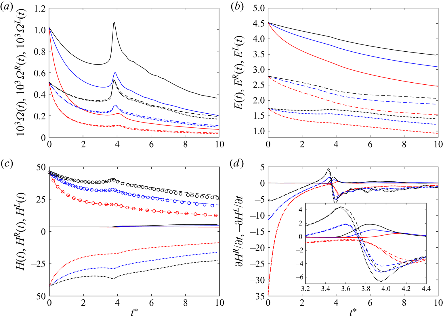
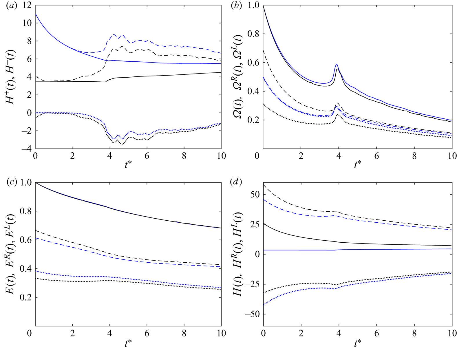
Figure 19(a) shows the evolution of enstrophy for the right- and left-handed components ( $\varOmega ^R$ and
 $\varOmega ^L$). Overall, both
 $\varOmega ^R$ and
 $\varOmega ^L$ have the same behaviour as the global enstrophy
 $\varOmega$: they decay initially and experience rapid growth during reconnection, followed by a rapid drop after reconnection. Initially,
 $\varOmega ^R$ and
 $\varOmega ^L$ have roughly the same magnitudes (approximately
 $\varOmega /2$), but become different as time progresses. Besides, the disparity between
 $\varOmega ^R$ and
 $\varOmega ^L$ increases with
 $Re$ – suggesting that the evolution of right- and left-handed polarized structures may become significantly different at sufficiently high
 $Re$. Figure 19(b) shows the evolution of energy for the total structures
 $E$ and the right- and left-handed components (
 $E^R$ and
 $E^L$). Due to viscous dissipation, the global energy
 $E(t)$ continuously decays, and the decay rate decreases with increasing
 $Re$. In addition,
 $E(t)$ decay faster during reconnection, which is due to the generations of small scales through intense stretching – consistent with a spike of
 $\varOmega (t)$ in figure 19(a). Note that the energy (and also helicity) for purely right- and left-polarized components are not conserved in inviscid flows (Chen, Chen & Eyink Reference Chen, Chen and Eyink2003). Hence,
 $E^R$ and
 $E^L$ can decrease due to viscous dissipation or being transferred to the other. As the trefoil vortex knot is predominately right-hand polarized,
 $E^R(t)$ is larger than
 $E^L(t)$. While
 $E^R(t)$ continuously decreases similar to
 $E(t)$, the decay rate during reconnection is even faster than
 $E(t)$. It means that there is an energy transfer from the right-handed component to the left-handed one, which causes
 $E^L(t)$ for the two high
 $Re$ cases to slightly increase during reconnection.
Time evolution of (a) enstrophy, (b) energy, (c) helicity and (d) rate of change of helicity for right-hand (dashed) and left-hand (dotted) polarized structures at  $Re=2000$ (red),
 $6000$ (blue) and
 $12\,000$ (black). The global enstrophy, energy and helicity, which are the sum of right- and left-hand components, are shown in (a–c). Note that the circles in (c) denote
 $-H^L(t)+H(0)$, with
 $H(0)=3.52$ the initial global helicity.

The helicity for right- and left-handed polarized components ( $H^R$ and
 $H^L$) as a function of
 $t^*$ is displayed in figure 19(c). Note that due to the negative sign of
 $H^L$, the increase of
 $H^L$ indicates the annihilation of the left-handed polarized structures. The evolution of
 $H^R$ and
 $H^L$ are much smoother compared with those of
 $H^\pm$ shown in figure 12(b). It is interesting that
 $H^R(t)$ and
 $H^L(t)$ behave quite similar to those of
 $\varOmega ^R$ and
 $\varOmega ^L$. Before reconnection,
 $H^R$ (or
 $H^L$) exponentially decay (grow) due to viscous dissipation and slightly increase (decrease) during reconnection, and decay (grow) again after reconnection. However, the growth and decay rates are different between
 $H^R$ and
 $H^L$, which results in complicated behaviours of
 $H$ observed in figure 3. To further explore this point, figure 19(d) shows the rate of change of helicity for right- and left-handed components (
 $\partial H^R/\partial t$ and
 $-\partial H^R/\partial t$). Here, negative (positive) value denotes the diminish (enhance) of polarized structures. Consistent with the continuous decaying of
 $H^R$ and growth of
 $H^L$ for
 $Re=2000$,
 $\partial H^R/\partial t$ and
 $-\partial H^L/\partial t$ remain negative all the time. For
 $Re=6000$ and
 $12\,000$ cases, both
 $\partial H^R/\partial t$ and
 $-\partial H^L/\partial t$ increase and become positive before reconnection – consistent with the generation of polarized structures shown in figure 13(a). Besides,
 $\partial H^R/\partial t$ and
 $-\partial H^L/\partial t$ are almost identical before the first peak but become different as reconnection starts. In particular,
 $-\partial H^L/\partial t$ is slightly lower than
 $\partial H^R/\partial t$, which again suggests that the left-handed polarized structures decay faster than the right-handed ones – resulting in an increase of
 $H$. The difference between
 $-\partial H^L/\partial t$ and
 $\partial H^R/\partial t$ increases with increasing
 $Re$, which is consistent with a more rapid increase of
 $H$ during reconnection at higher
 $Re$. After reconnection, the difference between
 $-\partial H^L/\partial t$ and
 $\partial H^R/\partial t$ slowly decreases for
 $Re=2000$; but persists over a very long time for the two high
 $Re$ cases. It confirms that the faster decay of left-handed polarized structures is the main cause of transient helicity growth at high
 $Re$.
4.5. Energy and helicity spectra
Figure 20(a,c,e) show the energy spectra at various instants for different  $Re$ cases. At
 $t^*=0$,
 $E(k)$ falls smoothly at high wavenumbers owing to the Gaussian profile of the vorticity distribution. Due to viscous dissipation,
 $E(k)$ at small wavenumbers (i.e.
 $k\le 50$) continuously decreases with time. However, at high wavenumbers a slight increase of
 $E(k)$ is observed for
 $t^*=4.45$, which is due to the generation of small scales, such as threads, during reconnection. After reconnection, these small scales rapidly decay at
 $Re=2000$ due to a strong viscous effect; hence, the energy at high wavenumbers quickly drops. An increase in
 $Re$ results in generating additional smaller scales; thus, the increase of
 $E(k)$ at high wavenumbers is more pronounced for high
 $Re$ cases. For
 $Re=12\,000$,
 $E(k)$ develops a power law close to
 $k^{-7/3}$ – akin to that observed by van Rees et al. (Reference van Rees, Hussain and Koumoutsakos2012) for anti-parallel reconnection of polarized vortex tubes. Furthermore, the energy drop becomes slower at higher
 $Re$ due to suppressed energy dissipation.
(a,c,e) Kinetic energy spectrum  $E(k)$ of the total structures and (b,d,f) helicity spectrum for the right- and left-handed components at several instants for: (a,b)
 $Re=2000$, (c,d)
 $6000$ and (e,f)
 $12\,000$.

The helicity spectra for the right-handed  $H^R(k)$ and left-handed
 $-H^L(k)$ components based on helical wave decomposition are displayed in figure 20(b,d,f). Note that for the pure right- and left-handed vortices, we have
 $H^R(k) = kE^R(k)$ and
 $H^L(k) = -kE^L(k)$ (Biferale, Musacchio & Toschi Reference Biferale, Musacchio and Toschi2012; Kessar et al. Reference Kessar, Plunian, Stepanov and Balarac2015). In addition, the Schwarz's inequality suggests that
 $|H(k)|\le kE(k)$. Overall, the evolution of
 $H^R(k)$ and
 $-H^L(k)$ are quite similar to that of
 $E(k)$. As the flow is predominant right-handed polarized,
 $H^L(k)$ at
 $t^*=0$ is slightly smaller than
 $-H^R(k)$ at low wavenumbers. Both
 $H^R(k)$ and
 $-H^L(k)$ have certain oscillations, which is consistent with that observed in Xiong & Yang (Reference Xiong and Yang2020) for initially twisted vortex knots. During the evolution, both
 $H^R(k)$ and
 $-H^L(k)$ decay at low wavenumbers. But they are manifested at high wavenumbers during reconnection, which is consistent with the generation of twist helicity in figure 14. At a given time, the helicity contents at high wavenumbers increase with
 $Re$. In addition,
 $-H^L(k)$ is always smaller than
 $H^R(k)$ at small wavenumbers, but is almost identical to
 $H^R(k)$ at very high wavenumbers. It indicates that fine-scale structures have no preference for polarization – agreeing with the conjecture by Brissaud et al. (Reference Brissaud, Frisch, Leorat, Lesieur and Mazure1973) that helicity has a negligible dynamical effect at sufficiently high wavenumbers. However, it is interesting to note that at moderate wavenumbers (i.e.
 $k\approx 100$),
 $-H^L(k)$ is slightly larger than
 $H^R(k)$. This is consistent with more numerous small-scale negative
 $h$ structures, mainly due to the stretching of SLR by LTR (figures 13c and 15c).
5. Effect of initial twist
We have shown that the generation of twist can cause the global helicity to grow after reconnection for high  $Re$. In this section we further investigate the effect of twist on flow evolution via additional simulations of the trefoil vortex knotted with non-zero initial twist (i.e.
 $T_{w,0}=7.48$ and
 $22.48$). Figure 21 shows the time progression of flow structures visualized based on vorticity isosurface at
 $Re=2000$ and
 $6000$ for the
 $T_{w,0}=22.48$ case. The flow evolution is quite similar to that for the
 $T_{w,0}=0$ case, and the only apparent difference is the distribution of the helicity density, which also becomes quite similar at late times due to the rapid decay of twist helicity. The similarity in flow evolution is further confirmed in figure 22(a,b) where the length and writhe of the vortex at
 $Re=6000$ for the
 $T_{w,0}=22.48$ case are almost identical to those of the
 $T_{w,0}=0$ case. It suggests that compared with twist, the writhe plays a more important role in the evolution of knotted vortices. In addition, figure 22(c) shows that the centrelinehelicity
 $H_c$ agrees with
 $H$ before reconnection and becomes smaller than
 $H$ after reconnection. But the difference between them decreases with time.
Evolution of flow structures represented by vorticity isosurface at 4 % of maximum initial vorticity (shaded in colour with helicity density) for (a)  $Re=2000$ and (b)
 $Re=6000$ with
 $T_{w,0}=22.48$.

Time evolution of (a) the length  $l_c$, (b) the writhe
 $W_r$ and (c) the centreline helicity
 $H_c$ of the vortex knot before reconnection (circle), and for SLR (
 $\triangle$), LTR (
 $\triangledown$) and their sum (
 $\square$) for
 $Re=6000$ with initial twist
 $T_{w,0}=22.48$. Note that the solid lines in (a,b) are the total length and the helicity
 $W_r$ for
 $Re=6000$ with
 $T_{w,0}=0$ cases, and in (c) are the global helicity
 $H$ for
 $Re=6000$ with
 $T_{w,0}=22.48$.

Figure 23(a) shows the evolution of enstrophy  $\varOmega$ (normalized by its initial value
 $\varOmega _0$) for different initial twist cases. Overall, the evolution is quite similar to that of the
 $T_{w,0}=0$ cases. However, compared with the
 $T_{w,0}=0$ cases, the enstrophy
 $\varOmega$ decays faster as
 $T_w$ increases. In Appendix B we demonstrate that, for a rectilinear Batchelor vortex column, the decay rate of
 $\varOmega$ monotonously increases with the strength of twist. The faster decay of
 $\varOmega$ is also consistent with the claim that helicity can inhibit energy transfer due to its role in depleting nonlinear interaction (Wu et al. Reference Wu, Ma and Zhou2007). Besides, the time for the peak of
 $\varOmega$ to occur slightly increases as
 $T_{w,0}$ increases, which suggests that reconnection delays for strong
 $T_{w,0}$ cases. It is consistent with the previous finding that the self-induced velocity of the vortex is reduced by increasing axial flows (Virk, Hussain & Kerr Reference Virk, Hussain and Kerr1995; Cheng, Lou & Lim Reference Cheng, Lou and Lim2016).
Time evolution of (a) the enstrophy  $\varOmega$ and (b) global helicity
 $H$ for different initial twist and Reynolds numbers. The dashed lines in (a,b) denote
 $\varOmega (t)=\varOmega _0 \exp [-\int ^t_0(2\nu /\sigma ^2)]\,\textrm {d}t$ and
 $H(t)=\varGamma ^2W_r(0)+\varGamma ^2T_w(0) \exp [-\int ^t_0(2\nu /\sigma ^2)\,\textrm {d}t]$ with
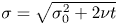 $\sigma =\sqrt {\sigma ^2_0+2\nu t}$, respectively.

The evolution of global helicity  $H$ for different initial twist cases is shown in figure 23(b). In contrast to the
 $T_{w,0}=0$ cases, where
 $H$ is mainly in the form of
 $W_r$ and is almost constant initially,
 $H$ rapidly decays for the
 $T_w\neq 0$ cases, and the decay rate increases with
 $T_w$. As discussed above, for a twisted straight vortex column,
 $T_w$ is dissipated at a rate
 $(1/T_w)\partial t/\partial T_w=-2\nu /\sigma ^2$ with
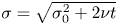 $\sigma =\sqrt {\sigma ^2_0+2\nu t}$. Hence, by assuming that writhe remains conserved, the helicity should roughly follow
 $H=\varGamma ^2 W_r(0)+\varGamma ^2T_w(0) \exp [-\int ^t_0(2\nu /\sigma ^2)]\,\textrm {d}t$. For all cases, the helicity evolution before reconnection agrees with the theoretical prediction based on the straight vortex. Different from the
 $T_{w,0}=0$ cases, the rapid increase of
 $H$ after reconnection is not observed. Instead,
 $H$ continuously decays for all the time, but the decay rate decreases after reconnection.
Figures 24(a) further shows the volume-integrated positive and negative helicities 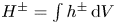 $H^{\pm }=\int h^{\pm } \,\mathrm {d}V$ for
 $Re=6000$ with
 $T_{w,0}=22.48$. Initially,
 $H^-$ is zero, indicating that all structures are associated with positive
 $h$. Similar to the
 $T_{w,0}=0$ case, structures with negative
 $h$ develop before reconnection; as a result,
 $H^-$ starts to increase and reach a peak around the time of reconnection. But compared with the
 $T_{w,0}=0$ case,
 $H^-$ decreases for
 $T_{w,0}=22.48$. The decrease of
 $H^-$ for strong
 $T_{w,0}$ cases seems to be consistent with the suppression of the energy cascade. Figure 24(b) shows the evolution of enstrophy of the right- and left-handed components (
 $\varOmega ^R$ and
 $\varOmega ^L$) for
 $Re=6000$ with
 $T_{w,0}=22.48$. Both
 $\varOmega ^R$ and
 $\varOmega ^L$ exhibit similar trends as those for the
 $T_{w,0}=0$ case. Since the knotted vortex is strongly right polarized,
 $\varOmega ^R$ is initially much larger than
 $\varOmega ^L$. In addition,
 $\varOmega ^R$ for the
 $T_{w,0}=22.48$ case is always larger than that for the
 $T_{w,0}= 0$ case, but the difference continuously decreases with time. Similarly,
 $\varOmega ^L$ for the
 $T_{w,0}=22.48$ case is always smaller than that for the
 $T_{w,0}=0$ case, and the difference decreases with time. Thus, although the vortices are initialized with different twists, the flow would eventually become identical. Figure 24(c) further compares the total energy and energy of the right- and left-handed components between the
 $T_{w,0}=0$ and
 $22.48$ cases. Despite a distinct difference of
 $\varOmega$ between these two cases, the evolution of
 $E(t)$ is visually identical. Similar to that of enstrophy,
 $E^R(t)$ is much larger than
 $E^L(t)$ initially, and both of them slowly approach the values of the
 $T_{w,0}=0$ case. From figure 24(d), it is clear that introducing twist enhances
 $H^R$ and suppresses
 $H^L$ simultaneously – suggesting that the flow becomes more Beltramized (i.e.
 $\boldsymbol {u}\|\boldsymbol {\omega }$). Due to its initial high value,
 $H^R$ decays faster than
 $H^L$, causing a rapid decrease of
 $H$. During reconnection, although both
 $H^R$ and
 $H^L$ increase, the increase of
 $H^R$ is slightly smaller than
 $H^L$ – causing
 $H$ to decrease. After reconnection,
 $H^R$ and
 $H^L$ decrease again and approach those of the
 $T_{w,0}=0$ case.
Time evolution of (a)  $H^{\pm }$, (b) enstrophy, (c) energy and (d) helicity for
 $Re=6000$ with
 $T_{w,0}=0$ (black) and
 $T_{w,0}=22.48$ (blue). The solid, dashed and dotted lines in (a) denote
 $H$,
 $H^+$ and
 $H^-$, respectively, and in (b–d) represent quantities for global, right-handed and left-handed components.

Figure 25(a) shows the energy spectra at various instants for  $Re=6000$ with
 $T_{w,0}=22.48$. The spectrum at
 $t^*=0$ has slight oscillations at high wavenumbers, similar to those observed for the right-handed components of the
 $T_{w,0}=0$ case (figure 20b). The evolution of
 $E(k)$ is almost identical to that of
 $T_{w,0}=0$ case, consistent with the identical energy evolution of these two cases. The helicity spectra of the right- and left-handed components for
 $Re=6000$ with
 $T_{w,0}=22.48$ are shown in figure 25(b). For all
 $k$,
 $-H^L(k)$ is initially smaller than
 $H^R(k)$. As time progresses, the difference between
 $-H^L(k)$ and
 $H^R(k)$ at small
 $k$ persists but decreases at high
 $k$. Consistent with the
 $T_{w,0}=0$ case,
 $-H^L(k)$ is larger than
 $H^R(k)$ at moderate
 $k$.
(a) Kinetic energy spectrum  $E(k)$ of the total structures and (b) helicity spectrum for the right- and left-handed components at several instants for
 $Re=6000$ and
 $T_{w,0}=22.48$ case. The insets in (a,b) show the comparison of
 $E(k)$ and
 $H^R(k)$ at
 $t^*=4.45$ between
 $T_{w,0}=0$ (solid) and
 $T_{w,0}=22.48$ (dashed) cases, respectively.

6. Concluding remarks
We performed direct numeral simulations of trefoil knotted vortices with different initial twists. Different from previous works (Scheeler et al. Reference Scheeler, Kleckner, Proment, Kindlmann and Irvine2014; Kerr Reference Kerr2018c), we observed that the global helicity  $H$ is not conserved for the zero initial twist cases. It slightly decreases before reconnection; and its evolution after reconnection strongly depends on
 $Re$: for the low
 $Re$ case, it slightly increases after reconnection, while for the high
 $Re$ case, it remarkably increases for a long time before finally decaying – suggesting that helicity is not conserved during viscous reconnection (even at very higher
 $Re$). The centreline helicity, calculated as
 $H_c=\sum _i \varGamma _i \oint _{\mathcal {C}_i} \boldsymbol {u}\boldsymbol {\cdot }\boldsymbol {T}(s)\,\textrm {d}s$, is found to be a good approximation for
 $H$ before and a long time after reconnection. In addition, the writhe
 $W_r$ continuously decreases before reconnection and becomes preserved after reconnection, akin to that found in quantum reconnection (Scheeler et al. Reference Scheeler, Kleckner, Proment, Kindlmann and Irvine2014). Different from the global helicity, the evolution of
 $W_r$ is almost
 $Re$ independent – suggesting that the strong twist helicity is generated at high
 $Re$.
Further analyses, such as flow visualization, helicity decomposition and helical wave decomposition, shows that significant amounts of positive and negative twist helicities are generated before and during reconnection. As the reconnection is asymmetric, the small leading and large trailing rings generated after reconnection are predominately negatively and positively twisted, respectively. Different from the straight vortex column, where the dissipation of twist  $\partial T_w/\partial t$ depends on viscosity, initial twist value and core size, the rate of twist dissipation for a coiled vortex ring also depends on the geometry, particularly the core size to radius ratio. Besides,
 $\partial T_w/\partial t$ is also influenced by mutual induction of the other ring. Due to the relatively large value of the initial twist,
 $\partial T_w/\partial t$ for LTR is larger than that in SLR at
 $Re=2000$ – resulting in a decrease of the total twist as well as global helicity. However, as
 $Re$ increases, the difference between initial twist decreases,
 $\partial T_w/\partial t$ for SLT becomes larger than that for LTR – causing a ‘transient’ net increase of
 $H$ at high
 $Re$.
In addition, reconnection of trefoil knotted vortices with different initial twist cases are considered. The flow structure evolution is quite similar to that of the zero initial twist case. In particular, the total length and the writhe are almost identical for different  $T_{w,0}$ cases. One apparent difference is that the enstrophy and the associated energy dissipation are suppressed for strong
 $T_{w,0}$ cases. The suppressed energy cascade is found to be associated with decreased generation of the left-handed polarized structures. The results suggest that although the writhe governs the evolution of knotted vortices, twist also plays an important role in flow dynamics, especially energy cascade and dissipation. In addition, the twist dissipation is strongly affected by the vortex core size. It would be interesting to investigate the effects of the radius of knots and core size on the reconnection dynamics. In addition, studies of single and interacting coiled vortex rings are required to better understand the mechanism of writhe and twist conversions.
Acknowledgements
Computational and visualization resources provided by Texas Tech University HPCC, TACC Lonestar, Frontera and Stampede2 under XSEDE are acknowledged.
Declaration of interests
The authors report no conflict of interest.
Appendix A. Grid convergence analysis for  $Re=2000$ and $6000$


A grid sensitivity analysis has been carried out for Reynolds numbers  $Re=2000$ and
 $6000$. For each
 $Re$, three different grid resolutions are tested, namely,
 $N^3=512^3$,
 $768^3$ and
 $1024^3$ for
 $Re=2000$; and
 $N^3=1536^3$,
 $2048^3$ and
 $3072^3$ for
 $Re=6000$. Figure 26(a) shows the time evolution of enstrophy
 $\varOmega$ for the three different grid resolutions at
 $Re=2000$ and
 $6000$. As
 $\varOmega$ is very sensitive to small-scale dynamics, the collapse of
 $\varOmega$ indicates that the resolutions we employed in the main text are sufficient to capture the small scales generated during the reconnection process. The evolution of the global helicity
 $H$ is shown in figure 26(b), where good agreements among different resolutions are also observed. Note that the small difference for the
 $Re=6000$ and
 $N^3=1536^3$ case after reconnection might be due to its insufficiency in capturing the axial velocity associated with the twist structures in the rings.
Time evolution of (a) enstrophy  $\varOmega$ and (b) global helicity
 $H$ for
 $Re=2000$ (red),
 $6000$ (blue) with different grid resolutions.

Appendix B. Enstrophy and helicity dissipation for a Batchelor vortex
Consider a straight Batchelor vortex (figure 27); its vorticity distribution is  $\boldsymbol {\omega }=[\omega _r, \omega _\theta , \omega _z]=[0, rqf, f]$, where
 $q$ quantifies the strength of the axial flow and
 $f$ is the axial vorticity distribution given in (2.10). The enstrophy dissipation rate is given as
 \begin{align} \frac{\partial \varOmega}{\partial t}={-}\nu \int (\boldsymbol{\nabla} \boldsymbol{\omega})^2 \,\textrm{d}V &=\nu\int [(\omega_\theta/r)^2+(\partial \omega_\theta/\partial r)^2+(\partial \omega_z/\partial r)^2]\,\textrm{d}V \end{align}
 \begin{align} &=\nu\int [2q^2f^2+(1+r^2q^2)f'^2+2rq^2ff']\,\textrm{d}V, \end{align}
which can be simplified as a relative decay rate
 \begin{equation} \frac{\partial \varOmega}{\partial t}={-}2\nu\varOmega\frac{2q^2\sigma^2+1}{(q^2\sigma^2+1)\sigma^2}. \end{equation}
Here  $\sigma$ is the vortex core scale and grows as
 $\sigma (t)=\sqrt {\sigma ^2_0+2\nu t}$ in a viscous flow. Note that the decay rate is
 $-2\nu \varOmega /\sigma ^2$ for the special
 $q=0$ case (Lamb–Oseen vortices), and asymptotically increases as
 $q$ increases. The rapid decay for the strong
 $q$ case is consistent with the claim that the helicity can suppress energy dissipation as
 $\epsilon =\nu \varOmega$.
Schematic illustration of the Batchelor vortex. Note that the red arrow represents the rotation direction of the vortex, and the purple line denotes the vortex lines.

Similarly, the helicity dissipation rate is
 \begin{equation} \frac{\partial H}{\partial t}={-}2\nu \int \boldsymbol{\omega} \boldsymbol{\cdot}(\boldsymbol{\nabla} \times \boldsymbol{\omega})\, \textrm{d}V={-}4\nu q \int f^2\, \textrm{d}V ={-}2\nu H/\sigma^2. \end{equation}
This dissipation depends on viscosity and core size. As the helicity is in the form of twist only, this is equivalent to a dissipation of the total twist ( $\partial T_w/\partial t=-2\nu T_w/\sigma ^2$).
Appendix C. Helicity evolution for two co-axial oppositely twisted vortex rings
We consider the dynamics of two co-axial oppositely twisted vortex rings undergoing a leap-frogging motion. The radii of inner and outer rings are  $R_i=0.5$ and
 $R_o=1$, respectively, and the circulation and the core size are the same as for the trefoil knot (i.e.
 $\varGamma =1$ and
 $\sigma =1/(16\sqrt {2{\rm \pi} })\approx 0.025$). The initial inner and outer rings are negatively and positively twisted, respectively, with the correspondingly initial twists
 $T^i_{w,0}=-9$ and
 $T^o_{w,0}=10$. The simulation is performed at
 $Re=6000$ with grid points
 $N^3=768^3$.
Figure 28 shows the evolution of global helicity along with the vortices visualized based on the isosurface of  $|\boldsymbol {\omega }|$. Note that as the writhe remains zero, the global helicity
 $H=\varGamma ^2T_w=\varGamma ^2(T^i_w+T^o_w)$. Here
 $T^i_w$ and
 $T^o_w$ denote the twist for the inner and outer rings, respectively. Following Appendix B, the dissipation rate of each ring is
 $\partial T_w/\partial t=-2\nu T_w/\sigma ^{2}(t)$, with
 $\sigma (t)$ denoting the core size. The two rings remain isolated during the evolution; hence, the circulation
 $\varGamma$ for each ring remains almost constant. Consequently, the dissipation rate of
 $H$ is
 \begin{equation} \frac{\partial H}{\partial t}={-}2\nu\varGamma^2\left(\frac{T^i_w}{\sigma_i^{2}(t)} +\frac{T^o_w}{\sigma_o^{2}(t)}\right), \end{equation}
which suggest that  $H$ can either increase or decrease, depending on the relative value between
 $T^i_w/\sigma ^2_i$ and
 $T^o_w/\sigma ^2_o$.
Time evolution of the global helicity  $H$ for the co-axial oppositely twisted vortex rings. Flow structures are represented by vorticity isosurface at 4 % of maximum initial vorticity shaded with positive (red) and negative (blue) helicity densities.

Initially, as two rings are in the same plane, stretching and compression are limited; hence, the core sizes of the rings are almost unchanged. Although the twist in both rings decays, the helicity decreases as the (positive) twist of the outer ring decays faster due to its larger initial value. However, when the inner ring advects sufficient far away from the outer ring, the inner and outer rings, respectively, undergo stretching and compression (as sketched in figure 17b). As a result, the core sizes of the inner and outer ring become smaller and larger, respectively; hence, the (negative) twist in the inner ring decays faster; therefore, the global helicity starts to grow. This is similar to the increase of twist and helicity for trefoil knot after reconnection, as shown in figure 3 and implied by (4.8). In the process of leap-frogging, the total twist and global helicity can sometimes increase or decrease, as the two rings have different decay rates based on whether they are compressed or stretched. Note that the interaction between SLR and LTR after trefoil knot reconnection is much more complicated than what we consider here. As these two rings are coiled, there are additional conversions between the writhe and twist helicity during successive compression or stretching of the two rings.