1 Introduction
Because of the prominent heat and mass transfer performance due to the large contact area, porous materials are widely used for various engineering devices such as catalytic converters, metal foam heat exchangers and gas diffusion layers for fuel cells (Nield & Bejan Reference Nield and Bejan2006; De Lemos Reference De Lemos2012). Hence, understanding the influence of the porous characteristics on turbulence around the porous media is crucial in industry. In particular, since the wall-blocking condition plays an important role in the dynamics of a turbulent boundary layer, several experimental and numerical studies have focused intensively on the effects of wall permeability, which reduces the effect of wall blocking.
Zagni & Smith (Reference Zagni and Smith1976) conducted Pitot tube experiments on turbulent open-channel flows over porous media composed of spheres. They found that the turbulent friction of permeable porous beds was higher than that of equivalent impermeable beds of the same surface roughness. Furthermore, they reported that, even in high-Reynolds-number regimes, the turbulent friction increased as the Reynolds number increased though the turbulent friction of the rough wall did not show a Reynolds-number dependence. Kong & Schetz (Reference Kong and Schetz1982) carried out similar experiments on the turbulent boundary layer over sintered metal, perforated titanium sheets and bonded screen sheets. They compared the turbulent friction of the porous wall with that of an impermeable wall of the same surface roughness and concluded that the increase of friction was due to the combined effects of wall permeability and roughness. Zippe & Graf (Reference Zippe and Graf1983) measured the velocity profiles of boundary-layer flows over porous beds composed of grains. They reached the same conclusions as Zagni & Smith (Reference Zagni and Smith1976) and Kong & Schetz (Reference Kong and Schetz1982) that the wall permeability increased turbulent friction. Moreover, they reported a meaningful discrepancy between the profiles of the streamwise turbulent intensity over permeable and impermeable walls.
Recent particle image velocimetry (PIV) experiments have made it possible to discuss turbulent flow structures in more detail. Pokrajac & Manes (Reference Pokrajac and Manes2009) measured turbulent flows over impermeable and permeable beds with identical surface roughness, which were both composed of uniform-size spheres packed in a cubic pattern. They summarized that, although the difference of the streamwise turbulence intensity of permeable and impermeable beds was not significant, the wall-normal turbulent intensity increased significantly due to the influence of the wall permeability. Manes et al. (Reference Manes, Pokrajac, McEwan and Nikora2009) carried out PIV measurements for turbulent open-channel flows over permeable and impermeable packed beds of spheres. They concluded that the rise of turbulent friction of the permeable wall could be attributed to shear penetration within the beds. They also discussed turbulent transport over permeable beds and reached the conclusion that turbulence produced over permeable beds was transported by turbulent velocity fluctuations in the upper part of the porous bed, whereas the pressure fluctuations allowed turbulence to be transported to much lower bed levels. Suga et al. (Reference Suga, Matsumura, Ashitaka, Tominaga and Kaneda2010) performed PIV measurements of porous-walled channel flows. To systematically investigate the effect of wall permeability on turbulence, they used three kinds of foamed ceramics, which had almost the same porosity but different permeabilities. To characterize turbulence over the permeable wall, they introduced a permeability Reynolds number
 $Re_{K}$
based on the friction velocity of the porous wall and the square root of the permeability. They found that, as the permeability Reynolds number increased, the wall-normal Reynolds stress was enhanced. This led to an increase of the turbulent shear stress, resulting in higher turbulent friction of permeable porous walls. It was reported that the enhancement of turbulence was remarkable in the range of
 $Re_{K}>3$
. They also found that
 $Re_{K}$
could reasonably characterize the roughness height, the zero-plane displacement and the Kármán constant. Furthermore, Suga, Mori & Kaneda (Reference Suga, Mori and Kaneda2011) discussed turbulent vortex structures over the permeable wall by quadrant analysis and concluded that the contribution of sweeps was the most dominant, whilst ejections tended to lose their strength very near the permeable porous wall. The superimposed effects of those motions and the Kelvin–Helmholtz (KH) type of instability were considered to result in shortening of the longitudinal vortical structures and the low-speed elongated streaks. This change of the structures was more obvious at a higher permeable Reynolds number
 $Re_{K}\gg 3$
. Manes, Poggi & Ridolfi (Reference Manes, Poggi and Ridolfi2011) also discussed the turbulent coherent structures over the permeable wall by performing laser Doppler velocimetry (LDV) of open-channel flows over high-porosity metal foams of different permeability. They concluded that, as the wall permeability increased, the coherence of the Reynolds shear stress increased, which resulted in the rise of the momentum transport efficiency. They also reported that a highly permeable wall allowed the development of large-scale eddies induced by the KH instability.
Those large-scale vortical structures originating from the KH instability have been extensively discussed in many studies on vegetation canopy flows (Raupach, Finnigan & Brunei Reference Raupach, Finnigan and Brunei1996; Finnigan Reference Finnigan2000; Ghisalberti & Nepf Reference Ghisalberti and Nepf2002; Poggi et al. Reference Poggi, Porporato, Ridolfi, Albertson and Katul2004). It was known that the flows near the vegetation canopy behaved like a perturbed mixing layer and the inflection of the mean velocity profiles caused the formation of large-scale coherent structures. This coherent structure was characterized by energetic sweeps and weakened ejections. This enhanced an exchange of momentum near the vegetation canopy.
From the above experimental studies, it is understood that, as the wall permeability increases, the wall-normal and Reynolds shear stresses increase, resulting in a higher turbulent friction. Furthermore, over highly permeable walls, large-scale vortical structure originating from the KH instability is induced and this enhances the momentum exchange over the permeable wall. However, because of the difficulty in performing measurements inside porous media, it is not easy to discuss the turbulent flow physics inside porous walls. Furthermore, discussion of the three-dimensional vortical structures is not easy. Accordingly, several direct numerical simulation (DNS) studies have been attempted. However, since enormous computational costs are required to resolve the complex porous structures, some numerical approaches which model the turbulence over a porous wall have been considered. The simplest approach is the specification of the wall boundary conditions. Jimenez et al. (Reference Jimenez, Uhlmann, Pinelli and Kawahara2001) performed DNS with a boundary condition allowing vertical fluid motion at the porous-wall interface. They imposed no-slip conditions for the streamwise and spanwise velocities, and set the wall-normal velocity to be proportional to the local pressure fluctuations. They found that the friction increased by up to 40 % over the walls, which was associated with the presence of large spanwise rollers, originating from linear instability related to the KH instability of shear layers. Hahn, Je & Choi (Reference Hahn, Je and Choi2002) applied slip velocity conditions in the streamwise and spanwise directions and set the wall-normal velocity to zero. These conditions did not relax the wall-blocking effect, unlike the boundary condition of Jimenez et al. (Reference Jimenez, Uhlmann, Pinelli and Kawahara2001). They reported that vortical structures were weakened over porous media and the Reynolds stresses simultaneously decreased, reducing the turbulent friction of the wall.
Since those approaches did not consider flows inside the porous media, the effect of the porous media on turbulence may not be precisely reproduced. To consider flows inside porous media with reasonable computational demands, Breugem, Boersma & Uittenbogaard (Reference Breugem, Boersma and Uittenbogaard2006) applied the volume-averaged Navier–Stokes (VANS) equations of Whitaker (Reference Whitaker1986, Reference Whitaker1996) to the porous region of porous-walled channel flows. Changing the permeability of the wall, they investigated the influence of the wall permeability on turbulence and found that elongated streaky structures and associated quasi-streamwise vortices were absent near a highly permeable wall (
 $Re_{K}\simeq 10$
), and significantly enhanced turbulence was dominant with relatively large vortical structures, which were supposed to originate from the KH instability. They concluded that this phenomenon enhanced the Reynolds shear stress and led to strong friction of a highly permeable wall whilst the enhancement of turbulence near an insufficiently permeable wall (
 $Re_{K}<1$
) was not significant. Samanta et al. (Reference Samanta, Vinuesa, Lashgari, Schlatter and Brandt2015) performed DNS of a porous square duct flow by using the VANS equations. They concluded that, because of the different interaction between the ejections from the side walls and the porous wall, the secondary flow intensity was significantly increased. Furthermore, although the side walls made the spanwise roll structure originated from the KH instability shorter, the spanwise rolls disturbed the development of the streamwise streaky structures over the porous wall.
However, since their VANS equation included the model for a drag force term and the effect of dispersion was neglected, turbulence phenomena around and inside the porous layers were not precisely reproduced. Accordingly, for more rigorous discussions, Chandesris et al. (Reference Chandesris, D’Hueppe, Mathieu, Jamet and Goyeau2013) and Kuwata & Suga (Reference Kuwata and Suga2016b
,Reference Kuwata and Suga
c
) recently performed full DNS, resolving each porous element. Kuwata & Suga (Reference Kuwata and Suga2016b
) conducted DNS of porous- and rough-walled turbulent channel flows to investigate the effects of wall permeability and wall roughness on turbulence separately. They considered staggered cube arrays for the porous wall and the same surface structures were considered for the rough wall. Over the permeable wall at
 $Re_{k}=3.8$
, they observed the less organized high- and low-speed streaks as reported by Breugem et al. (Reference Breugem, Boersma and Uittenbogaard2006). Moreover, their proper orthogonal decomposition analysis revealed the presence of spanwise transverse rolls of pressure induced by the KH instability over the porous and rough walls. The roll structure over the porous wall was more organized and energetic, and this intensified the wall-normal and spanwise velocity fluctuations, leading to a stronger turbulent shear over the permeable porous wall. Furthermore, through a budget term analysis of the volume-averaged turbulence equation for the same flow system of Kuwata & Suga (Reference Kuwata and Suga2016b
), Kuwata & Suga (Reference Kuwata and Suga2016c
) reported that significant pressure fluctuation over the porous wall reinforced the redistribution and pressure diffusion processes, which made turbulence more isotropic over the porous layer and carried turbulence vertically inside the porous layer.
The above DNS studies reveal the absence of elongated streaky structures over porous walls. They also discussed the presence and characteristics of the large-scale transverse roll structures induced by the KH instability over highly permeable walls. Furthermore, it was found that associated pressure fluctuation intensified the redistribution and pressure diffusion terms, which made turbulence more isotropic over the porous layer and carried turbulence vertically inside the porous layer.
Although the effect of wall permeability on turbulence has been extensively investigated to date, as far as the authors know, the discussions have been limited to isotropic porous media and the wall permeability has not been considered as a tensorial form. Hence, despite the wide range of applications of anisotropic porous materials in industry, such as rod bundles, fibrous media and layered media, it has not been clarified which component of the permeability tensor influences turbulence over porous walls. Therefore, this study discusses the influence of the anisotropic permeability tensor of porous media on turbulence by performing DNS of anisotropic permeable porous-walled channel flows using the D3Q27 multiple-relaxation-time (MRT) lattice Boltzmann method (LBM) of Suga et al. (Reference Suga, Kuwata, Takashima and Chikasue2015) with the imbalance correction local grid refinement method of Kuwata & Suga (Reference Kuwata and Suga2016a ). The presently used porous media have square hole arrays aligned with the Cartesian axes. To examine which component of the anisotropic permeability tensor of porous media influences turbulence over the porous wall, the permeability tensor is arbitrarily changed by introducing vertical, streamwise and spanwise hole arrays.
2 Numerical approach
Owing to the simplicity of the wall treatment and high computer efficiency, the LBM has become a popular tool for complex porous-medium flow simulations (e.g. Hatiboglu & Babadagli Reference Hatiboglu and Babadagli2008; Suga et al.
Reference Suga, Tanaka, Nishio and Murata2009; Suga & Nishio Reference Suga and Nishio2009; Beugre et al.
Reference Beugre, Calvo, Dethier, Crine, Toye and Marchot2010; Parmigiani et al.
Reference Parmigiani, Huber, Bachmann and Chopard2011; Chukwudozie & Tyagi Reference Chukwudozie and Tyagi2013). Furthermore, since the LBM is suitable for parallel computing using the Message Passing Interface and Graphics Processing Units as reported by Li et al. (Reference Li, Zhang, Wang and Ge2013) and Huang et al. (Reference Huang, Shi, He and Chai2015) and has been validated for turbulent flow DNS (e.g. Lammers et al.
Reference Lammers, Beronov, Volkert, Brenner and Durst2006; Chikatamarla et al.
Reference Chikatamarla, Frouzakis, Karlin, Tomboulides and Boulouchos2010; Bespalko, Pollard & Uddin Reference Bespalko, Pollard and Uddin2012; Suga et al.
Reference Suga, Kuwata, Takashima and Chikasue2015), it has often been applied to various complex turbulent flow problems such as flows in porous media (e.g. Hasert, Bernsdorf & Roller Reference Hasert, Bernsdorf and Roller2011; Krafczyk et al.
Reference Krafczyk, Kucher, Wang and Geier2015; Kuwata & Suga Reference Kuwata and Suga2015b
) or over rough walls (e.g. Jin, Uth & Herwig Reference Jin, Uth and Herwig2015; Tóth & Jánosi Reference Tóth and Jánosi2015; Kuwata & Suga Reference Kuwata and Suga2016b
,Reference Kuwata and Suga
c
). Because of the above distinctive computational features, this study employs the LBM for simulating the time-dependent turbulent flow fields over porous walls. The lattice Boltzmann equation can be obtained by discretizing the velocity space of the Boltzmann equation into a finite number of discrete velocities
 $\unicode[STIX]{x1D743}_{\unicode[STIX]{x1D6FC}}\{\unicode[STIX]{x1D6FC}=0,\ldots ,Q-1\}$
. There are several discrete velocity models for three-dimensional flow simulations such as the D3Q15, D3Q19 and D3Q27 models.
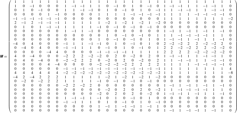
It has been reported that, although unphysical spurious currents were sometimes visible in the D3Q15 and D3Q19 models in axisymmetric flows, they were effectively suppressed by the D3Q27 model (White & Chong Reference White and Chong2011; Kang & Hassan Reference Kang and Hassan2013; Kuwata & Suga Reference Kuwata and Suga2015a ). Also, to ensure numerical stability for high-Reynolds-number flows, it is effective to apply the MRT scheme (D’Humiéres et al. Reference D’Humiéres, Ginzburg, Krafczyk, Lallemand and Luo2002). Accordingly, the present study employs the D3Q27 MRT-LBM of Suga et al. (Reference Suga, Kuwata, Takashima and Chikasue2015). The time evolution of the distribution function of the MRT-LBM can be written as
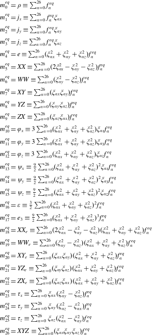
 $$\begin{eqnarray}|\boldsymbol{f}(\boldsymbol{x}+\unicode[STIX]{x1D743}_{\unicode[STIX]{x1D6FC}}\unicode[STIX]{x1D6FF}t,t+\unicode[STIX]{x1D6FF}t)\!\rangle -|\boldsymbol{f}(\boldsymbol{x},t)\!\rangle =-\unicode[STIX]{x1D648}^{-1}\hat{\unicode[STIX]{x1D64E}}[|\boldsymbol{m}(\boldsymbol{x},t)\!\rangle -|\boldsymbol{m}^{eq}(\boldsymbol{x},t)\!\rangle ],\end{eqnarray}$$
where the notation such as
 $|\boldsymbol{f}\!\rangle$
means
 $|\boldsymbol{f}\!\rangle =(f_{0},f_{1},\ldots ,f_{Q-1})^{\text{T}}$
and
 $\unicode[STIX]{x1D6FF}t$
is the time step. Note that for the D3Q27 model,
 $Q=27$
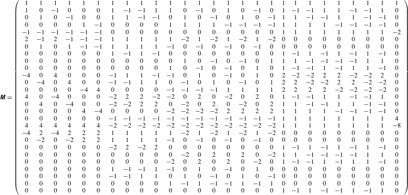
. The parameters for the D3Q27 model are listed in table 1. The matrix
 $\unicode[STIX]{x1D648}$
is a
 $Q\times Q$
matrix which linearly transforms the distribution functions to the moments as
 $|\boldsymbol{m}\!\rangle =\unicode[STIX]{x1D648}|\boldsymbol{f}\!\rangle$
. The equilibrium moment
 $\boldsymbol{m}^{eq}$
is obtained as
 $|\boldsymbol{m}^{eq}\!\rangle =\unicode[STIX]{x1D648}|\boldsymbol{f}^{eq}\!\rangle$
with
 $$\begin{eqnarray}f_{\unicode[STIX]{x1D6FC}}^{eq}=w_{\unicode[STIX]{x1D6FC}}\left(\unicode[STIX]{x1D70C}+\unicode[STIX]{x1D70C}_{0}\left[\frac{\unicode[STIX]{x1D743}_{\unicode[STIX]{x1D6FC}}\boldsymbol{\cdot }\boldsymbol{u}}{c_{s}^{2}}+\frac{(\unicode[STIX]{x1D743}_{\unicode[STIX]{x1D6FC}}\boldsymbol{\cdot }\boldsymbol{u})^{2}-c_{s}^{2}|\boldsymbol{u}|^{2}}{2c_{s}^{4}}\right]\right),\end{eqnarray}$$
where
 $\boldsymbol{u}$
is the fluid velocity and
 $\unicode[STIX]{x1D70C}$
is expressed as the sum of constant and fluctuation terms,
 $\unicode[STIX]{x1D70C}=\unicode[STIX]{x1D70C}_{0}+\unicode[STIX]{x1D6FF}\unicode[STIX]{x1D70C}$
(He & Luo Reference He and Luo1997). The sound speed is
 $c_{s}/c=1/\sqrt{3}$
with
 $c=\unicode[STIX]{x1D6E5}/\unicode[STIX]{x1D6FF}t$
where
 $\unicode[STIX]{x1D6E5}$
is the lattice spacing and the values of
 $w_{\unicode[STIX]{x1D6FC}}$
are listed in table 1. The equilibrium moments and the transformation matrix are shown in tables 2 and 3. The collision matrix
 $\hat{\unicode[STIX]{x1D64E}}$
is diagonal:
 $$\begin{eqnarray}\displaystyle \hat{\unicode[STIX]{x1D64E}} & \equiv & \displaystyle \text{diag}(\!0,0,0,0,s_{4},s_{5},s_{5},s_{7},s_{7},s_{7},s_{10},s_{10},s_{10},s_{13},s_{13},s_{13},\nonumber\\ \displaystyle & & \displaystyle \qquad s_{16},s_{17},s_{18},s_{18},s_{20},s_{20},s_{20},s_{23},s_{23},s_{23},s_{26}\! ).\end{eqnarray}$$
The relaxation parameters are
 $$\begin{eqnarray}\left.\begin{array}{@{}c@{}}s_{4}=1.54,\quad s_{5}=s_{7},\quad s_{10}=1.5,\quad s_{13}=1.83,\quad s_{16}=1.4,\\ s_{17}=1.61,\quad s_{18}=s_{20}=1.98,\quad s_{23}=s_{26}=1.74.\end{array}\right\}\end{eqnarray}$$
Parameters of the D3Q27 discrete velocity model.

Equilibrium moments.
 $\unicode[STIX]{x1D70C}$
, density;
 $j_{x},j_{y},j_{z}$
, momentum;
 $e$
, kinetic energy;
 $XX$
,
 $WW$
,
 $XY$
,
 $YZ$
,
 $ZX$
, second-order tensors;
 $\unicode[STIX]{x1D711}_{x},\unicode[STIX]{x1D711}_{y},\unicode[STIX]{x1D711}_{z}$
, flux of the energy;
 $\unicode[STIX]{x1D713}_{x},\unicode[STIX]{x1D713}_{y},\unicode[STIX]{x1D713}_{z}$
, flux of the square of the energy;
 $\unicode[STIX]{x1D700}$
, square of the energy;
 $e_{3}$
, cube of the energy;
 $XX_{e},WW_{e}$
, product of
 $XX$
and
 $WW$
by the energy;
 $XY_{e},YZ_{e},ZX_{e}$
, extra-diagonal second-order moments of the energy;
 $\unicode[STIX]{x1D70F}_{x},\unicode[STIX]{x1D70F}_{y},\unicode[STIX]{x1D70F}_{z}$
, third-order pseudo-vector;
 $XYZ$
, third-order totally antisymmetric tensor.
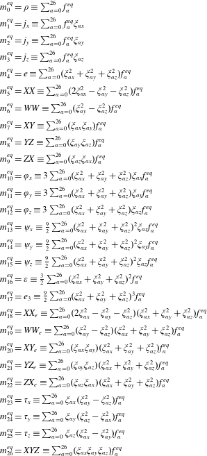
The
 $27\times 27$
transformation matrix.
The relaxation parameters
 $s_{5}$
and
 $s_{7}$
are related to the kinematic viscosity
 $\unicode[STIX]{x1D708}$
,
 $$\begin{eqnarray}\unicode[STIX]{x1D708}=c_{s}^{2}\left(\frac{1}{s_{5}}-\frac{1}{2}\right)\unicode[STIX]{x1D6FF}t=c_{s}^{2}\left(\frac{1}{s_{7}}-\frac{1}{2}\right)\unicode[STIX]{x1D6FF}t.\end{eqnarray}$$
The presently applied scheme of the D3Q27 MRT-LBM was validated in the application to the DNS of the turbulent channel flow of Kim, Moin & Moser (Reference Kim, Moin and Moser1987) at
 $Re_{\unicode[STIX]{x1D70F}}=180$
. The turbulence statistics, including the higher-order turbulence correlations such as the budget terms of the turbulent kinetic energy equation and the predicted energy spectra, showed almost perfect agreement with those by the spectrum method. Hence, the accuracy of this D3Q27 MRT-LBM was confirmed to be equivalent to that of the spectral method (see Suga et al.
Reference Suga, Kuwata, Takashima and Chikasue2015).
3 Flow geometry and computational conditions
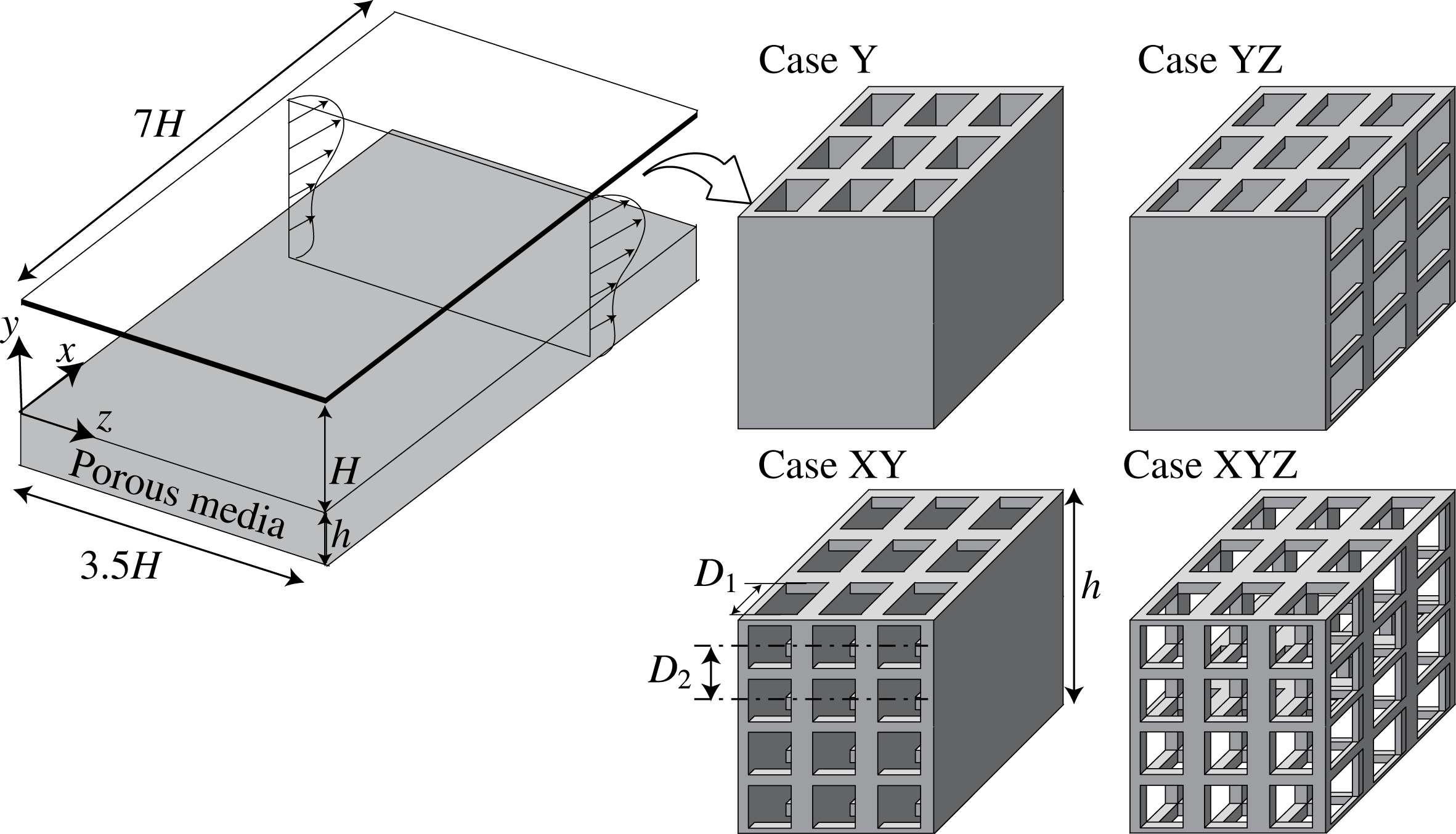
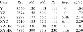
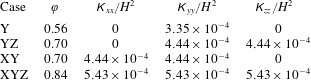
Figure 1 illustrates the computational geometries of porous-walled channel flows. The channel bottom wall is made of a porous medium whilst a solid smooth top wall is set. As shown in figure 1, the porous media presently considered (cases Y, YZ, XY and XYZ) have square pore arrays aligned with the Cartesian axes. All cases have vertical square pores. The streamwise and spanwise pores are also made in cases XY and YZ, respectively. For case XYZ, the vertical, streamwise and spanwise pores are made. The porous-medium thickness is
 $h=4D_{2}$
. The size and the pitch of the square holes are
 $D_{1}=0.116H$
and
 $D_{2}=1.50D_{1}$
, respectively. Since flows over porous media are principally influenced by two factors, namely the wall roughness and the wall permeability, to examine the individual influence of the two factors, DNS of rough-wall turbulence are also conducted. The presently focused two rough walls of cases YZ-R and XY-R have respectively the same structures as the cases YZ and XY; however, the wall thickness is thinned down to
 $h=D_{2}$
.
Computational geometry of porous-walled channel flows.

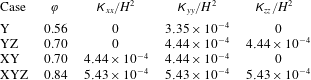
Characteristic parameters of porous media.
In the volume-averaged momentum equation (Whitaker Reference Whitaker1986) for fully developed homogeneous porous-medium flows, the volume-averaged pressure difference is balanced with the drag force, which is usually modelled as the Darcy–Forchheimer equation:
 $$\begin{eqnarray}\frac{1}{\unicode[STIX]{x1D70C}}\frac{\unicode[STIX]{x2202}\langle p\rangle ^{f}}{\unicode[STIX]{x2202}x_{i}}=\unicode[STIX]{x1D708}\unicode[STIX]{x1D711}\langle u_{j}\rangle ^{f}\unicode[STIX]{x1D612}^{ij}+\unicode[STIX]{x1D708}\unicode[STIX]{x1D711}\unicode[STIX]{x1D612}^{ij}\unicode[STIX]{x1D60D}_{jk}\langle u_{k}\rangle ^{f},\end{eqnarray}$$
where
 $\unicode[STIX]{x1D711}$
is the porosity,
 $\unicode[STIX]{x1D612}^{ij}$
denotes the inverse matrix of the permeability tensor
 $\unicode[STIX]{x1D612}_{ij}$
and
 $\unicode[STIX]{x1D60D}_{ij}$
denotes the Forchheimer tensor. The value
 $\langle \unicode[STIX]{x1D713}\rangle ^{f}$
is the fluid-phase (intrinsic) averaged value. For sufficiently low-Reynolds-number flows, the viscous drag becomes dominant and thus (3.1) may be reduced to
 $$\begin{eqnarray}\frac{1}{\unicode[STIX]{x1D70C}}\frac{\unicode[STIX]{x2202}\langle p\rangle ^{f}}{\unicode[STIX]{x2202}x_{i}}=\unicode[STIX]{x1D708}\unicode[STIX]{x1D711}\langle u_{j}\rangle ^{f}\unicode[STIX]{x1D612}^{ij}.\end{eqnarray}$$
To obtain the permeability tensor
 $\unicode[STIX]{x1D612}_{ij}$
by (3.2), which is one of the important characteristic parameters for porous-wall turbulence (Breugem et al.
Reference Breugem, Boersma and Uittenbogaard2006; Suga et al.
Reference Suga, Matsumura, Ashitaka, Tominaga and Kaneda2010; Kuwata & Suga Reference Kuwata and Suga2016b
), laminar flow simulations of fully developed porous-medium flows are preliminarily performed. The obtained diagonal components of the permeability tensor
 $\unicode[STIX]{x1D612}_{ii}$
and the porosity
 $\unicode[STIX]{x1D711}$
are shown in table 4. Note that the off-diagonal components of
 $\unicode[STIX]{x1D612}_{ij}$
become zero in the present coordinate system. The computational domain size
 $x\times y\times z$
of
 $L_{x}\times L_{y}\times L_{z}$
is set to
 $7.0H\times (H+h)\times 3.5H$
. Using the imbalance correction zonal grid refinement method of Kuwata & Suga (Reference Kuwata and Suga2016a
), which can remove the mass and momentum imbalances generated at fine and coarse grid interfaces, the computational domain is decomposed into finer and coarser resolution domains. The finer mesh domain mainly covers inside and around the porous-wall region of
 $-h/H\leqslant y/H<0.25$
, whilst the coarser mesh domain covers the other clear channel flow region of
 $0.25\leqslant y/H\leqslant 1.0$
. Periodic boundary conditions are applied to the streamwise and spanwise directions with a constant streamwise pressure difference. For no-slip boundaries, which are applied to the surfaces of the smooth top wall, the bottom of the porous wall and the porous elements, the half-way bounce-back method is used. Simulations are performed under a constant pressure difference at the averaged friction Reynolds number
 $Re_{\unicode[STIX]{x1D70F}}=u_{\unicode[STIX]{x1D70F}}H/2\unicode[STIX]{x1D708}=111$
. For cases XY and YZ, to discuss Reynolds-number dependence, higher-Reynolds-number simulations at
 $Re_{\unicode[STIX]{x1D70F}}=230$
(cases XY-HR and YZ-HR) are also carried out. Here, the averaged friction velocity is
 $u_{\unicode[STIX]{x1D70F}}=\sqrt{0.5((u_{\unicode[STIX]{x1D70F}}^{p})^{2}+(u_{\unicode[STIX]{x1D70F}}^{t})^{2})}$
, where the friction velocities of the smooth top wall and the porous bottom wall are
 $u_{\unicode[STIX]{x1D70F}}^{t}$
and
 $u_{\unicode[STIX]{x1D70F}}^{p}$
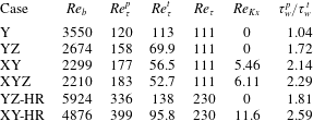
, respectively. The bulk Reynolds number
 $Re_{b}=U_{b}H/\unicode[STIX]{x1D708}$
, the streamwise permeability Reynolds number
 $Re_{Kx}=u_{\unicode[STIX]{x1D70F}}^{p}\sqrt{K_{xx}}/\unicode[STIX]{x1D708}$
, and the friction Reynolds numbers on the solid and bottom walls defined respectively as
 $Re_{\unicode[STIX]{x1D70F}}^{t}=u_{\unicode[STIX]{x1D70F}}^{t}\unicode[STIX]{x1D6FF}_{t}/\unicode[STIX]{x1D708}$
and
 $Re_{\unicode[STIX]{x1D70F}}^{p}=u_{\unicode[STIX]{x1D70F}}^{p}\unicode[STIX]{x1D6FF}_{p}/\unicode[STIX]{x1D708}$
are listed in table 5. The notations
 $\unicode[STIX]{x1D6FF}_{t}$
and
 $\unicode[STIX]{x1D6FF}_{p}$
denote the boundary-layer thicknesses of the smooth top and porous bottom walls, which are defined as
 $\unicode[STIX]{x1D6FF}_{t}/H=(u_{\unicode[STIX]{x1D70F}}^{t})^{2}/[(u_{\unicode[STIX]{x1D70F}}^{t})^{2}+(u_{\unicode[STIX]{x1D70F}}^{p})^{2}]$
and
 $\unicode[STIX]{x1D6FF}_{p}/H=(u_{\unicode[STIX]{x1D70F}}^{p})^{2}/[(u_{\unicode[STIX]{x1D70F}}^{t})^{2}+(u_{\unicode[STIX]{x1D70F}}^{p})^{2}]$
, respectively. The grid node numbers of the finer and coarser mesh regions at
 $Re_{\unicode[STIX]{x1D70F}}=111$
are
 $481\,(x)\times 130\,(y)\times 961\,(z)$
and
 $241\,(x)\times 55\,(y)\times 481\,(z)$
, respectively. Those in the higher-Reynolds-number case of
 $Re_{\unicode[STIX]{x1D70F}}=230$
are
 $981\,(x)\times 260\,(y)\times 1920\,(z)$
and
 $481\,(x)\times 110\,(y)\times 961\,(z)$
, respectively. The grid resolution of the finer mesh is set to
 $\unicode[STIX]{x1D6E5}^{f}u_{\unicode[STIX]{x1D70F}}^{p}/\unicode[STIX]{x1D708}<2.0$
which is comparable resolution to that employed in the previous DNS studies by the LBM (Chikatamarla et al.
Reference Chikatamarla, Frouzakis, Karlin, Tomboulides and Boulouchos2010; Bespalko et al.
Reference Bespalko, Pollard and Uddin2012; Suga et al.
Reference Suga, Kuwata, Takashima and Chikasue2015; Kuwata & Suga Reference Kuwata and Suga2016b
,Reference Kuwata and Suga
c
). Grid independence is confirmed by comparing turbulent intensities with those obtained by the 1.5 times denser mesh computation. The computational domain size is also validated by comparing turbulent intensities with those by the simulation of the larger box of
 $14.0H\,(x)\times (H+h)\,(y)\times 7H\,(z)$
. Further validation by comparing the turbulent statistics with the experimental data of Suga et al. (Reference Suga, Matsumura, Ashitaka, Tominaga and Kaneda2010) is discussed in appendix A.
Flow characteristics of the simulation.
The friction velocity of the smooth top wall
 $u_{\unicode[STIX]{x1D70F}}^{t}$
can be directly computed whilst the averaged friction velocity at the porous interface
 $u_{\unicode[STIX]{x1D70F}}^{p}$
is estimated by the balance between the pressure drop
 $\unicode[STIX]{x0394}P$
and the averaged wall shear stresses of the porous and top walls (
 $\unicode[STIX]{x1D70F}_{w}^{p}=\unicode[STIX]{x1D70C}(u_{\unicode[STIX]{x1D70F}}^{p})^{2}$
and
 $\unicode[STIX]{x1D70F}_{w}^{t}=\unicode[STIX]{x1D70C}(u_{\unicode[STIX]{x1D70F}}^{t})^{2}$
, respectively) as
 $$\begin{eqnarray}(\unicode[STIX]{x1D70F}_{w}^{p}+\unicode[STIX]{x1D70F}_{w}^{t})L_{x}L_{z}=HL_{z}\unicode[STIX]{x0394}P.\end{eqnarray}$$
Thus,
 $u_{\unicode[STIX]{x1D70F}}^{p}$
is given as
 $$\begin{eqnarray}u_{\unicode[STIX]{x1D70F}}^{p}=\left(-(u_{\unicode[STIX]{x1D70F}}^{t})^{2}+\frac{\unicode[STIX]{x0394}PH}{\unicode[STIX]{x1D70C}L_{x}}\right)^{0.5}.\end{eqnarray}$$
In the following discussions, the superscripts ‘
 $(~)^{t+}$
’ and ‘
 $(~)^{p+}$
’ indicate the values normalized by
 $u_{\unicode[STIX]{x1D70F}}^{t}$
and
 $u_{\unicode[STIX]{x1D70F}}^{p}$
, respectively.
4 Results and discussion
4.1 Mean velocity and Reynolds stresses
Owing to the spatial variation of wall structures, flows near porous media or rough walls do not always become homogeneous in a certain plane parallel to a wall. Hence, to statistically discuss such flows, spatial averaging has been introduced (Nikora et al.
Reference Nikora, Goring, McEwan and Griffiths2001; Franca, Ferreira & Lemmin Reference Franca, Ferreira and Lemmin2008; Hurther & Lemmin Reference Hurther and Lemmin2008; Mignot, Hurther & Barthelemy Reference Mignot, Hurther and Barthelemy2009). The definition of the spatial (plane) averaging of
 $\unicode[STIX]{x1D719}(x,y,z)$
is introduced as
 $$\begin{eqnarray}[\unicode[STIX]{x1D719}]^{f}(y)=\frac{1}{A_{S_{f}}}\int _{S}\unicode[STIX]{x1D719}(x,y,z)\,\text{d}S,\end{eqnarray}$$
where
 $S$
and
 $A_{S_{f}}$
are the surface of the
 $x{-}z$
plane and the surface areas of the fluid phase contained within
 $S$
, respectively. To discuss turbulence statistics around the porous walls, double averaging, which consists of the plane and Reynolds averaging operations, is applied. In the following discussions,
 $\overline{\unicode[STIX]{x1D719}}$
denotes the Reynolds-averaged value and
 $\unicode[STIX]{x1D719}^{\prime }$
denotes the fluctuated value from
 $\overline{\unicode[STIX]{x1D719}}$
. For the Reynolds averaging, simulations are carried out over 30 (
 $Re_{\unicode[STIX]{x1D70F}}=111$
) or 10 (
 $Re_{\unicode[STIX]{x1D70F}}=230$
) cycle times after the flows reach the fully developed states.
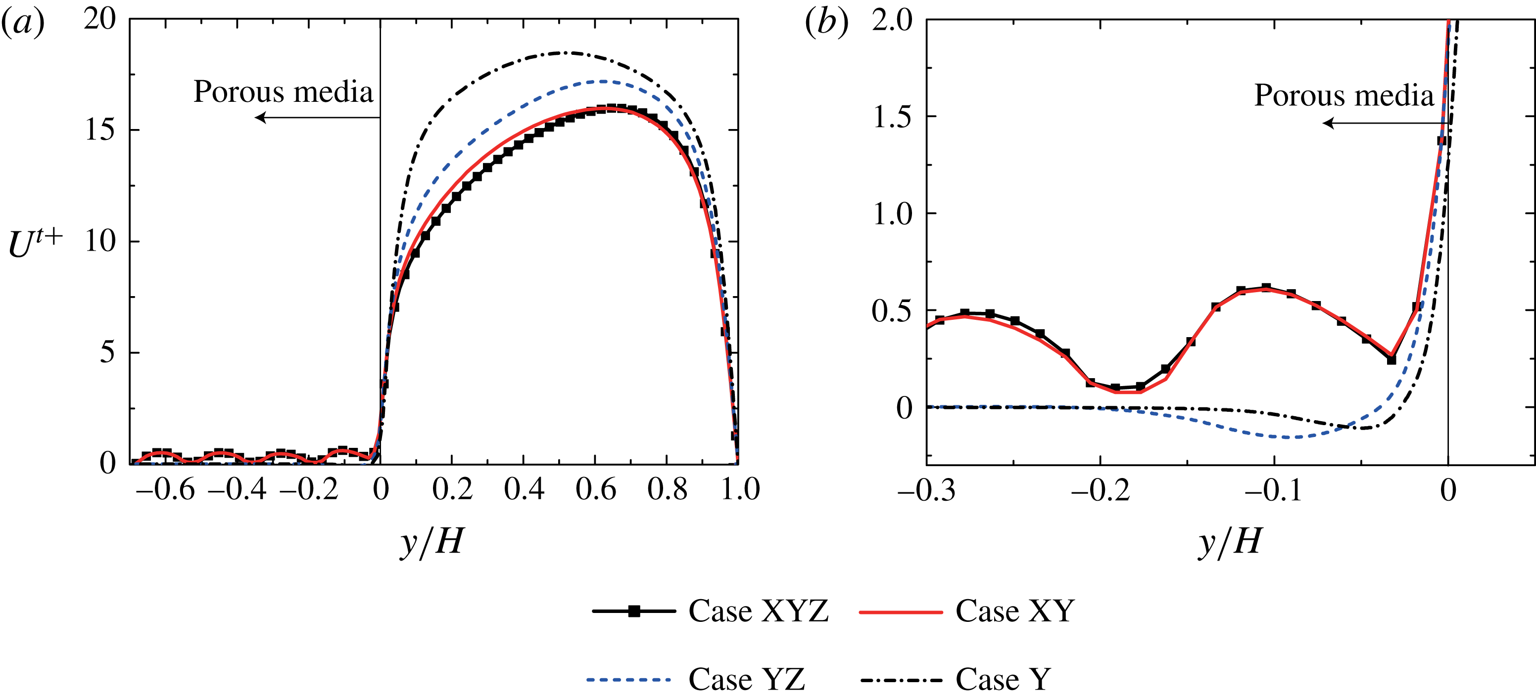
Plane-averaged streamwise mean velocity profiles normalized by
 $u_{\unicode[STIX]{x1D70F}}^{t}$
: (a) in porous and clear flow region; and (b) near the porous interface.

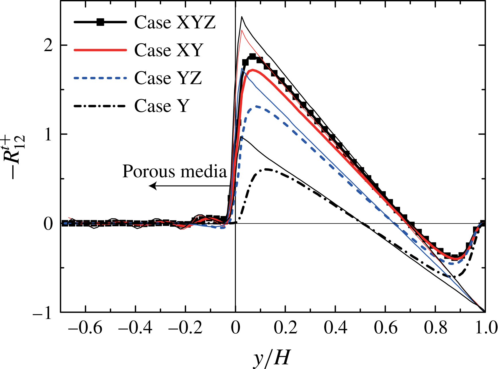
Figures 2 and 3 show the
 $x{-}z$
plane-averaged streamwise mean velocity
 $U^{t+}=[\overline{u}]^{f}/u_{\unicode[STIX]{x1D70F}}^{t}$
and Reynolds shear stress
 $R_{12}^{t+}=-[\overline{u^{\prime }v^{\prime }}]^{f}/(u_{\unicode[STIX]{x1D70F}}^{t})^{2}$
profiles normalized by the friction velocity of the smooth top wall. Therefore, in figure 3, the total stress reaches
 $-1$
at the top solid wall in all cases. Over the porous wall with spanwise and streamwise permeabilities (cases YZ, YZ and XYZ),
 $R_{12}^{t+}$
is significantly enhanced compared with that near the smooth top wall. In particular, the enhancement of
 $R_{12}^{t+}$
over the porous wall with streamwise permeability (cases XY and XYZ) is more pronounced than that in case YZ. Consequently, as shown in table 5, the enhancement of the wall shear stress of the porous wall
 $\unicode[STIX]{x1D70F}_{w}^{p}/\unicode[STIX]{x1D70F}_{w}^{t}$
in case XY is
 $1.28$
times larger than that in case YZ. As
 $R_{12}^{t+}$
increases, the friction Reynolds number of the porous-wall side
 $Re_{\unicode[STIX]{x1D70F}}^{p}$
increases, whereas the bulk mean Reynolds number
 $Re_{b}$
decreases; see table 5. In contrast, in case Y with pores only in the vertical direction,
 $U^{t+}$
rapidly converges to zero and the mean flow hardly penetrates into the bottom wall. Hence, even though the bottom wall is thick enough to neglect the influence of most of the bottom wall, the porous medium in case Y behaves as a rough wall. Furthermore, the pores of the bottom wall in case Y are so narrow that stable recirculation vortices that isolate the outer layer are sustained. Such flow is usually observed inside d-type roughness (Perry, Schofield & Joubert Reference Perry, Schofield and Joubert1969); thus it can be deduced that the bottom-wall characteristics hardly affect turbulence over the wall. Accordingly, the magnitudes of
 $R_{12}^{t+}$
in case Y over the porous and smooth top walls are almost the same and the profile of
 $U^{t+}$
in figure 2(a) is consequently almost symmetrical. Thus, as shown in table 5, the enhancement of the wall shear stress of the porous wall
 $\unicode[STIX]{x1D70F}_{w}^{p}/\unicode[STIX]{x1D70F}_{w}^{t}$
in case Y is
 $4\,\%$
at most. Figure 2(b) enlarges the plane-averaged mean velocity profiles beneath the porous interface. Although a slip velocity can be seen at the porous interface in all cases, that in case Y is smaller than those in cases XY, YZ and XYZ. Mean adverse flow can be seen just beneath the porous interface in cases YZ and Y; however, it eventually converges to zero inside the porous wall of
 $y/H<-0.2$
. The positive slip velocity and adverse flow just beneath the porous interface mean the presence of recirculation vortices just beneath the porous interface in cases Y and YZ. On the other hand,
 $U^{t+}$
in cases XY and XYZ does not converge to zero due to the streamwise permeability of the porous walls. The profiles in cases XY and XYZ are wavy corresponding to the porous structure, and clearly exhibit an inflection point (
 $\text{d}^{2}U/\text{d}y^{2}=0$
), which obeys a necessary condition for the inviscid instability such as the KH instability. The presence of the inflection point of the streamwise mean velocity was also reported by the DNS study for porous-walled channel flows (Breugem et al.
Reference Breugem, Boersma and Uittenbogaard2006; Kuwata & Suga Reference Kuwata and Suga2016b
,Reference Kuwata and Suga
c
) and experiments for vegetated canopy flows (Finnigan Reference Finnigan2000; Ghisalberti & Nepf Reference Ghisalberti and Nepf2002; Poggi et al.
Reference Poggi, Porporato, Ridolfi, Albertson and Katul2004).
Reynolds and total shear stress profiles normalized by
 $u_{\unicode[STIX]{x1D70F}}^{t}$
. The thin lines are the profiles of the total shear stress.

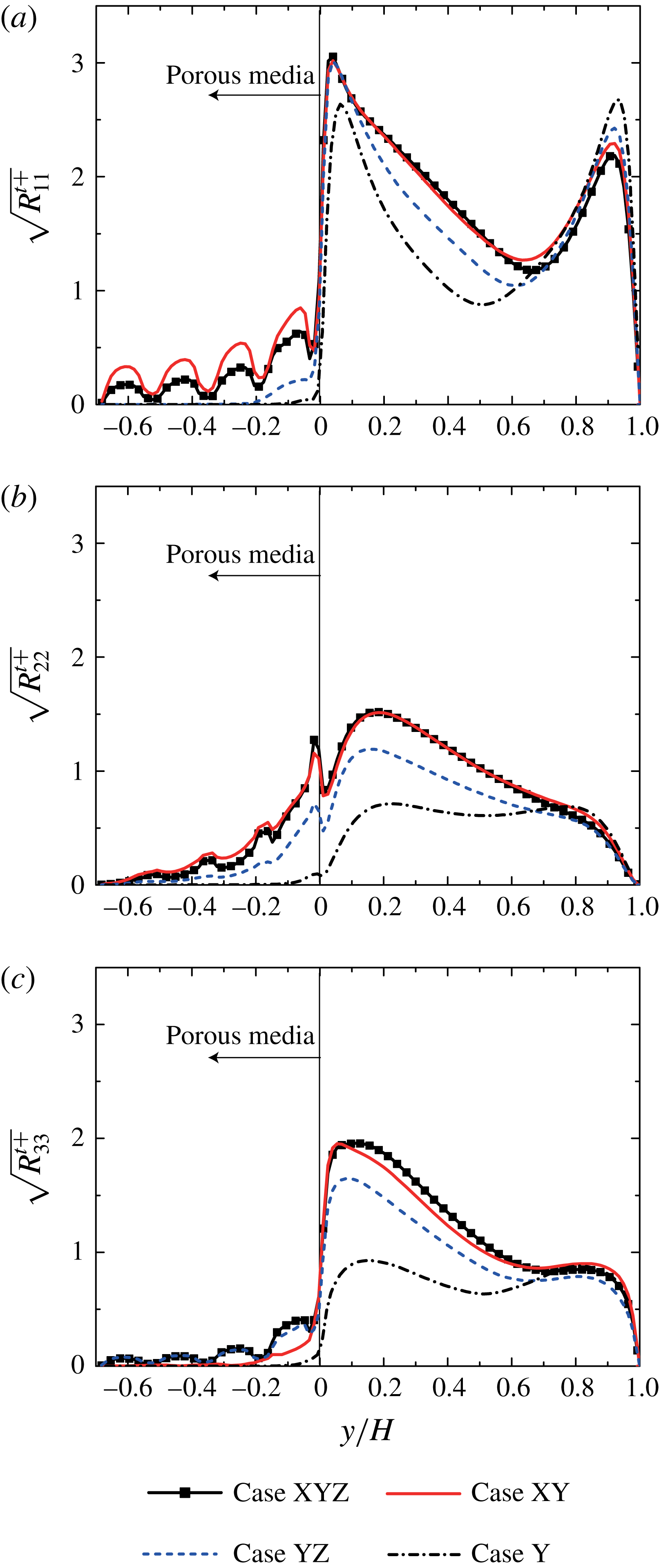
Plane-averaged Reynolds normal stresses normalized by
 $u_{\unicode[STIX]{x1D70F}}^{t}$
: (a) streamwise component, (b) wall-normal component, and (c) spanwise component.

Figure 4 presents profiles of the
 $x{-}z$
plane-averaged Reynolds normal stresses
 $R_{ij}^{t+}=[\overline{u_{i}^{\prime }u_{j}^{\prime }}]^{f}/(u_{\unicode[STIX]{x1D70F}}^{t})^{2}$
normalized by the friction velocity of the smooth top wall. Note that, since
 $R_{ij}^{t+}$
is almost damped at the bottom of the porous wall, the porous-wall thickness is enough to neglect the effect of the most bottom boundary of the porous wall. The plane-averaged Reynolds normal stresses of
 $R_{ij}^{t+}$
in case Y near the porous and smooth top walls are almost the same whilst
 $R_{ij}^{t+}$
near the porous wall in cases YZ, XY and XYZ are enhanced. The enhancement of
 $R_{11}^{t+}$
in figure 4(a) is less prominent compared with that of
 $R_{22}^{t+}$
and
 $R_{33}^{t+}$
in figure 4(b,c). It is consistent with the previous experiments of Pokrajac & Manes (Reference Pokrajac and Manes2009), Manes et al. (Reference Manes, Pokrajac, McEwan and Nikora2009) and Suga et al. (Reference Suga, Matsumura, Ashitaka, Tominaga and Kaneda2010) and the DNS of Breugem et al. (Reference Breugem, Boersma and Uittenbogaard2006) and Kuwata & Suga (Reference Kuwata and Suga2016b
). The local maximum values of
 $R_{11}^{t+}$
in proximity to the porous interface are almost the same level in cases XY, YZ and XYZ; however, approaching the channel centre,
 $R_{11}^{t+}$
in case YZ decreases more rapidly than those in cases XY and XYZ. Since
 $R_{ij}^{t+}$
over the streamwise permeable wall in cases XY are more enhanced than those over the spanwise permeable wall in case YZ, it can be deduced that the streamwise permeability particularly contributes to the increase of
 $R_{ij}^{t+}$
over the porous walls. Moreover, it is interesting to note that, regardless of the difference of the porous structures between cases XY and XYZ, the profiles of
 $R_{ij}^{t+}$
over the porous wall are very similar. Inside the porous wall,
 $R_{ij}^{t+}$
in case Y is almost damped whereas
 $R_{ij}^{t+}$
in cases XY, YZ and XYZ still remains. However, in case YZ, since streamwise permeability
 $K_{xx}$
becomes zero, streamwise fluid motion is restricted and
 $R_{11}^{t+}$
consequently becomes zero. Likewise for
 $R_{11}^{t+}$
in case YZ,
 $R_{33}^{t+}$
in case XY converges to zero inside the porous wall. Since the significant pressure diffusion transports
 $R_{22}^{t+}$
deep inside the porous wall, as reported by Kuwata & Suga (Reference Kuwata and Suga2016c
),
 $R_{22}^{t+}$
in cases YZ, XY and XYZ decays slower than
 $R_{11}^{t+}$
and
 $R_{33}^{t+}$
.
Comparisons of the mean values between the porous-wall and rough-wall results: (a)
 $U^{t+}$
and (b)
 $R_{12}^{t+}$
.

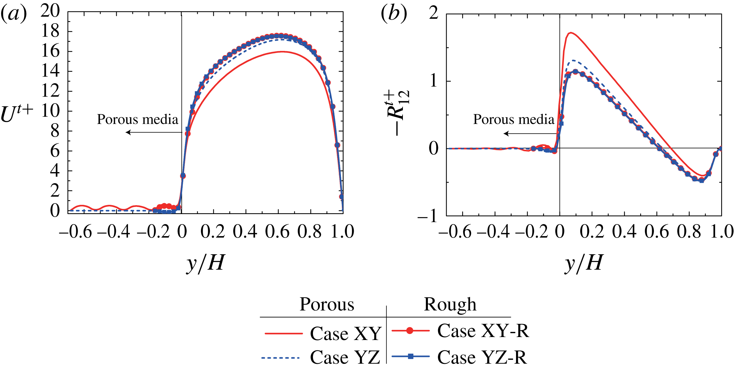
It should be noted that the above-discussed difference between the cases YZ and XY may be due to the difference of the wall roughness. To discuss the individual influence of the porous-wall roughness and permeability, figure 5 presents comparisons of the
 $x{-}z$
plane-averaged mean velocity
 $U^{t+}$
and Reynolds shear stress
 $R_{12}^{t+}$
profiles between the porous-wall cases (cases XY and YZ) and the rough-wall cases (cases XY-R and YZ-R). It is found that, although significant differences of
 $U^{t+}$
as shown in figure 5(a) can be observed between the cases XY and YZ, the mean velocity profiles over the different rough walls of cases XY-R and YZ-R almost overlap. Furthermore, in figure 5(b), enhancement of
 $R_{12}^{t+}$
by the porous wall is more remarkable than that by the rough walls. This implies that, as well as the wall roughness, the wall permeability itself significantly enhances turbulence. However, the Reynolds shear stress enhancement caused by the spanwise permeability in case YZ is less pronounced than that by the streamwise permeability in case XY. This suggests that the influence of the wall roughness in cases XY and YZ are almost the same whereas the remarkable enhancement of turbulence in case XY can be attributed to the streamwise permeability. It should be stressed that the impact of the anisotropic permeability on turbulence may be in contrast to that of the anisotropic rough walls. It was reported by the systematic DNS study of Orlandi, Leonardi & Antonia (Reference Orlandi, Leonardi and Antonia2006) that the roughness elements placed along the spanwise direction such as transverse ribs caused more drag increase than those placed along the streamwise direction. Moreover, it has been reported that drag reduction is even possible over the streamwise roughness elements, which are known as riblets (Bushnell Reference Bushnell1990; Goldstein, Handler & Sirovich Reference Goldstein, Handler and Sirovich1995).
4.2 Turbulence structures
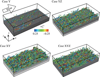
Figure 6 displays isosurfaces of the second invariant of the velocity gradient tensor of
 $II^{t+}=0.025$
normalized by
 $u_{\unicode[STIX]{x1D70F}}^{t}$
, which are coloured based on the local values of the streamwise vorticity of
 $-0.25<\unicode[STIX]{x1D714}_{x}^{t+}<0.25$
. Although a few vortices are visualized in case Y, strong vortex motions are observed over the porous wall in cases XY and YZ. The vortex motion seems to be more active in case XY than that in case YZ, and the vortex generation in case XY seems to be of roughly the same level as that in case XYZ.
Isosurfaces of the second invariant of the velocity gradient tensor
 $II^{t+}=0.025$
, coloured by the streamwise vorticity; blue–red colours correspond to
 $-0.25<\unicode[STIX]{x1D714}_{x}^{t+}<0.25$
.

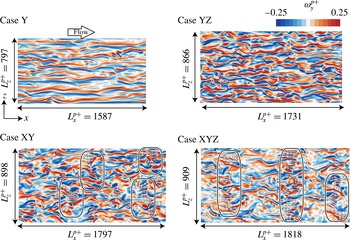
Figure 7 shows snapshots of the wall-normal vorticity fluctuations normalized by
 $u_{\unicode[STIX]{x1D70F}}^{p}$
over the porous walls at
 $y^{p+}\approx 13$
. The streamwise elongated streaky structure, which is usually observed over a smooth solid wall, is also observed in case Y whilst the elongated structure looks shredded and twisted in case YZ. Moreover, the streaky structures completely vanish in cases XY and XYZ, which is consistent with the vortex structures over a highly permeable wall reported by the DNS of Breugem et al. (Reference Breugem, Boersma and Uittenbogaard2006) and Kuwata & Suga (Reference Kuwata and Suga2016b
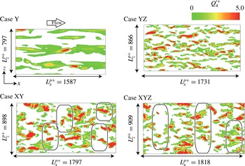
). Although a strong mean velocity gradient is present in cases XY and XYZ as shown in figure 2, which is required to form high- and low-speed streaks, the streaky structure in cases XY and XYZ vanishes. It is considered that the active wall-normal velocity fluctuation as shown in figure 4(b) prevents the development of the elongated streaky structures. Furthermore, it is observed in cases XY and XYZ that the vortex structure is intermittently shrunken, as indicated by the region enclosed by black solid lines in figure 7.
Snapshots of the instantaneous wall-normal vorticity fluctuations normalized by
 $u_{\unicode[STIX]{x1D70F}}^{p}$
at
 $y^{p+}\approx 13$
.

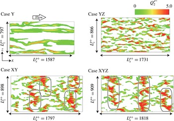
Snapshots of the instantaneous ejection distributions normalized by
 $u_{\unicode[STIX]{x1D70F}}^{p}$
at
 $y^{p+}\approx 13$
.

To discuss the turbulence structures over the porous wall in detail, figures 8 and 9 present snapshots of the instantaneous ejections
 $Q_{2}^{\prime p+}=-(u^{\prime }v^{\prime })^{p+}$
(
 $u^{\prime }<0$
and
 $v^{\prime }>0$
) and sweeps
 $Q_{4}^{\prime p+}=-(u^{\prime }v^{\prime })^{p+}$
(
 $u^{\prime }>0$
and
 $v^{\prime }<0$
) over the porous walls at
 $y^{p+}\approx 13$
, respectively. Note that all visualizations in figures 6–9 are made by the same snapshots. The region enclosed by black solid lines indicates the same region as shown in figure 7. Likewise for the distribution of the wall-normal vorticity fluctuations in figure 7, both the ejection and sweep structures are elongated in case Y and they are both shredded in case YZ. In cases XY and XYZ, the structures are no longer elongated to the streamwise direction. On the contrary, they tend to be merged in the spanwise direction. The active
 $Q_{2}^{\prime p+}$
regions in cases XY and XYZ seem to periodically emerge and the streamwise pitch is roughly 500–800 porous-wall units. However, this feature cannot be observed in the sweep structures in cases XY and XYZ in figure 9. Since the active
 $Q_{2}^{\prime +}$
regions in cases XY and XYZ correspond to the regions where the vortices are intermittently and periodically shrunken as seen in figure 7, they are caused by the low-speed fluid pushed up from the porous media in cases XY and XYZ. Furthermore, it was reported by Kuwata & Suga (Reference Kuwata and Suga2016b
) that strong transverse wavy pressure fluctuations induced by the KH instability accelerated or decelerated fluid inside the porous wall, and this leads to large-scale velocity fluctuations. Since those large-scale velocity fluctuations are pushed up from the porous wall, the intermittent patched structures appear only in ejections, not sweeps.
Snapshots of the instantaneous sweep distributions normalized by
 $u_{\unicode[STIX]{x1D70F}}^{p}$
at
 $y^{p+}\approx 13$
.

4.3 Two-point correlation analysis
To investigate turbulence structures over the porous walls in more detail, streamwise and spanwise two-point correlations over the porous walls at
 $y^{p+}\approx 13$
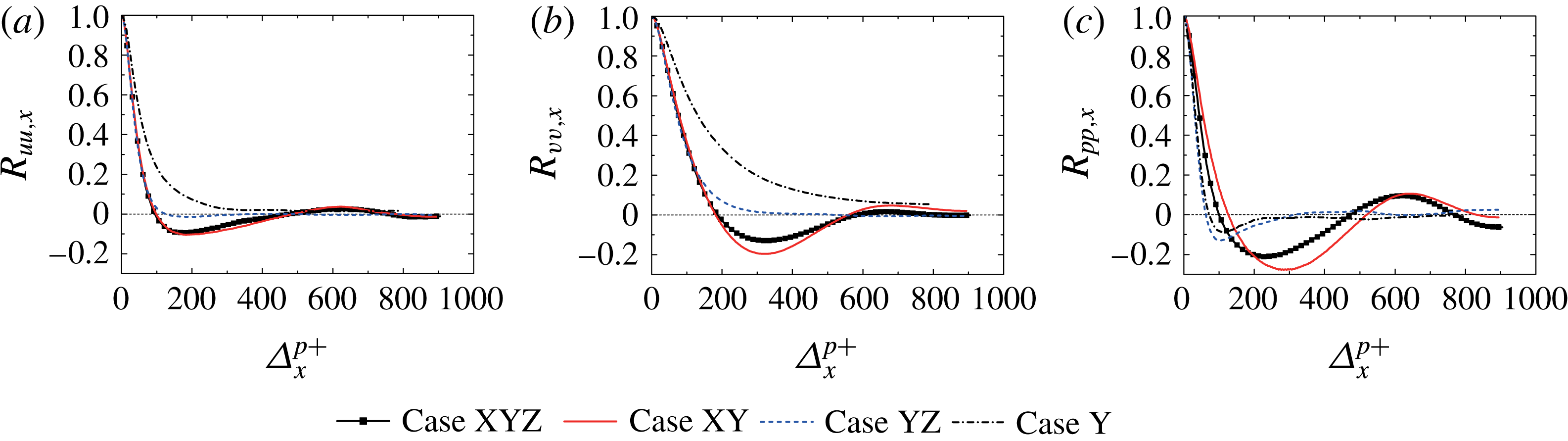
are shown in figures 10 and 11. In figure 10(a,b), the streamwise correlations of
 $R_{uu,x}$
and
 $R_{vv,x}$
in cases YZ, XY and XYZ decay more rapidly compared with those in case Y. This substantiates the reduction of the streamwise elongated streaky structures as observed in figure 7. The correlations
 $R_{uu,x}$
and
 $R_{vv,x}$
in case YZ converge to zero, whilst, in cases XY and XYZ, both
 $R_{uu,x}$
and
 $R_{uu,z}$
show a wavy profile and a negative local minimum around
 $\unicode[STIX]{x0394}x^{p+}=200{-}300$
is observed. Such a negative local minimum can also be seen in the streamwise pressure correlation
 $R_{pp,x}$
as shown in figure 10(c). This is considered to be due to the streamwise large-scale perturbation induced by the KH instability as reported by the DNS of Jimenez et al. (Reference Jimenez, Uhlmann, Pinelli and Kawahara2001), Breugem et al. (Reference Breugem, Boersma and Uittenbogaard2006) and Kuwata & Suga (Reference Kuwata and Suga2016b
) and the experiments of Finnigan (Reference Finnigan2000), Ghisalberti & Nepf (Reference Ghisalberti and Nepf2002) and Poggi et al. (Reference Poggi, Porporato, Ridolfi, Albertson and Katul2004). From these results, it is found that the streamwise permeability allows development of the streamwise perturbation by the KH instability, which is triggered by the inflection of the streamwise mean velocity as seen in figure 2. The representative wavelength of this perturbation estimated by the location of the local minimum is approximately
 $600$
porous-wall units and this roughly corresponds to the pitch of the intermittent patched patterns of the ejections in figure 8. It is noticeable that, although pores in case XY are not interconnected in the spanwise direction, the negative local minimum value of the streamwise pressure correlation around
 $\unicode[STIX]{x0394}x^{p+}=200{-}300$
in case XY is slightly more significant than that in case XYZ whose pores are interconnected in the spanwise direction. This implies that flow communications in the spanwise direction do not enhance the coherence of the streamwise perturbation whereas those in the streamwise direction are essential to sustain the streamwise perturbation.
Streamwise two-point correlations: (a) streamwise velocity fluctuations
 $R_{uu,x}$
, (b) wall-normal velocity fluctuations
 $R_{vv,x}$
, and (c) pressure fluctuations
 $R_{pp,x}$
.

Spanwise two-point correlations: (a) streamwise velocity fluctuations
 $R_{uu,z}$
, (b) wall-normal velocity fluctuations
 $R_{vv,z}$
, and (c) pressure fluctuations
 $R_{pp,z}$
.

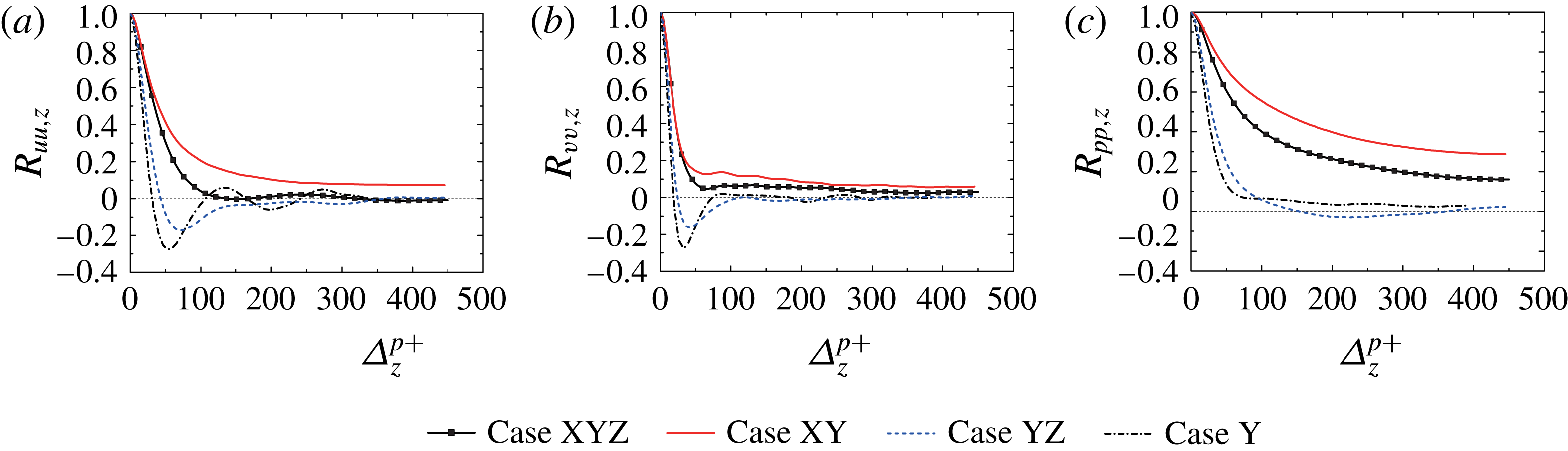
In figure 11, it is observed that the spanwise correlations
 $R_{uu,z}$
and
 $R_{vv,z}$
in cases Y and YZ exhibit a negative local minimum at
 $\unicode[STIX]{x1D6E5}_{z}^{p+}\approx 50$
, which is associated with the averaged spanwise distance of the high- and low-speed streaks. On the other hand, in cases XY and XYZ, such a negative local minimum cannot be observed in
 $R_{uu,z}$
and
 $R_{vv,z}$
. This suggests that the array of high- and low-speed streaks fades out in cases XY and XYZ, which is consistent with the observation in figure 7 and the previous DNS of Breugem et al. (Reference Breugem, Boersma and Uittenbogaard2006) and Kuwata & Suga (Reference Kuwata and Suga2016b
). In cases XY and XYZ, the spanwise correlation of
 $R_{pp,z}$
in figure 11(c) reaches a plateau, which implies the spanwise coherence across the full box. This result is consistent with the result of Jimenez et al. (Reference Jimenez, Uhlmann, Pinelli and Kawahara2001) and this spanwise coherence is considered to be due to the presence of the transverse pressure rolls by the KH instability as reported by Kuwata & Suga (Reference Kuwata and Suga2016b
).
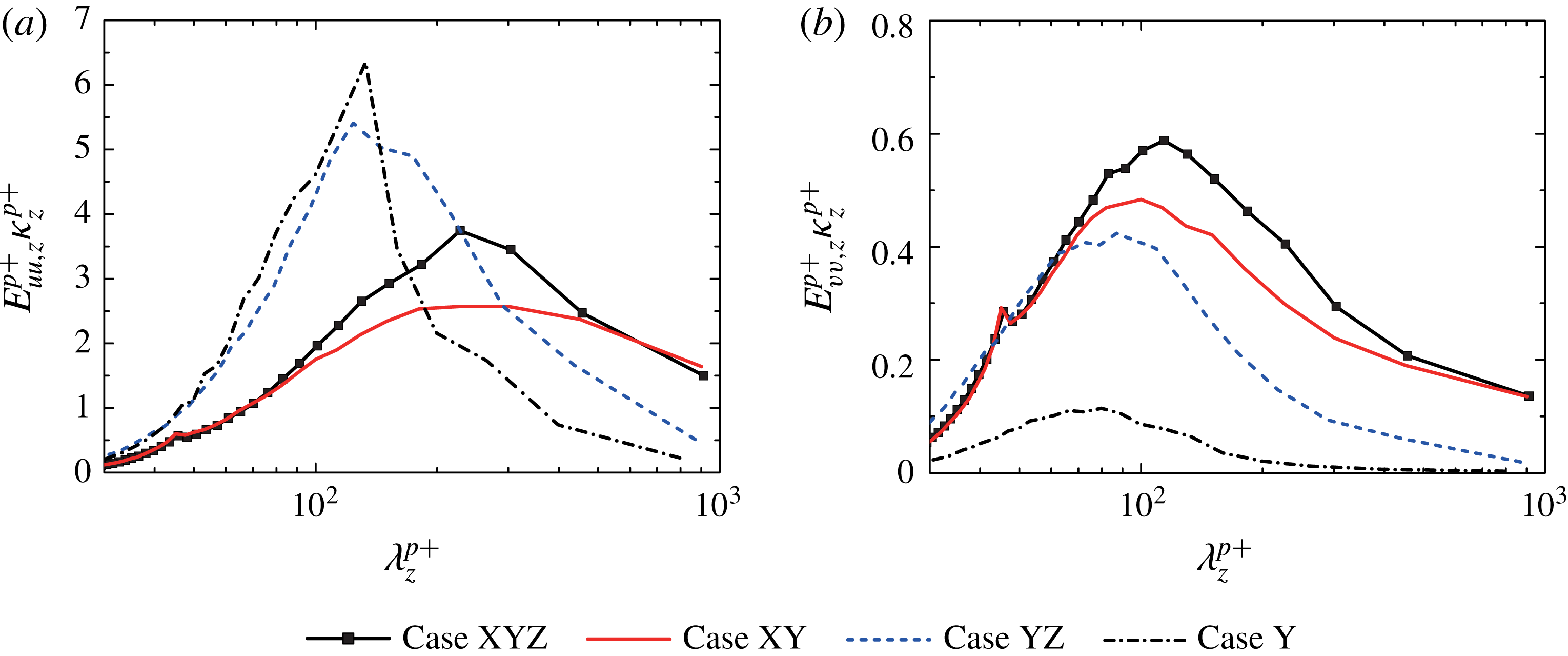
Premultiplied streamwise spectra: (a) streamwise velocity fluctuation
 $E_{uu,x}$
and (b) wall-normal velocity fluctuation
 $E_{vv,x}$
.

Premultiplied spanwise spectra: (a) streamwise velocity fluctuation
 $E_{uu,z}$
and (b) wall-normal velocity fluctuation
 $E_{vv,z}$
.

4.4 Spectral analysis
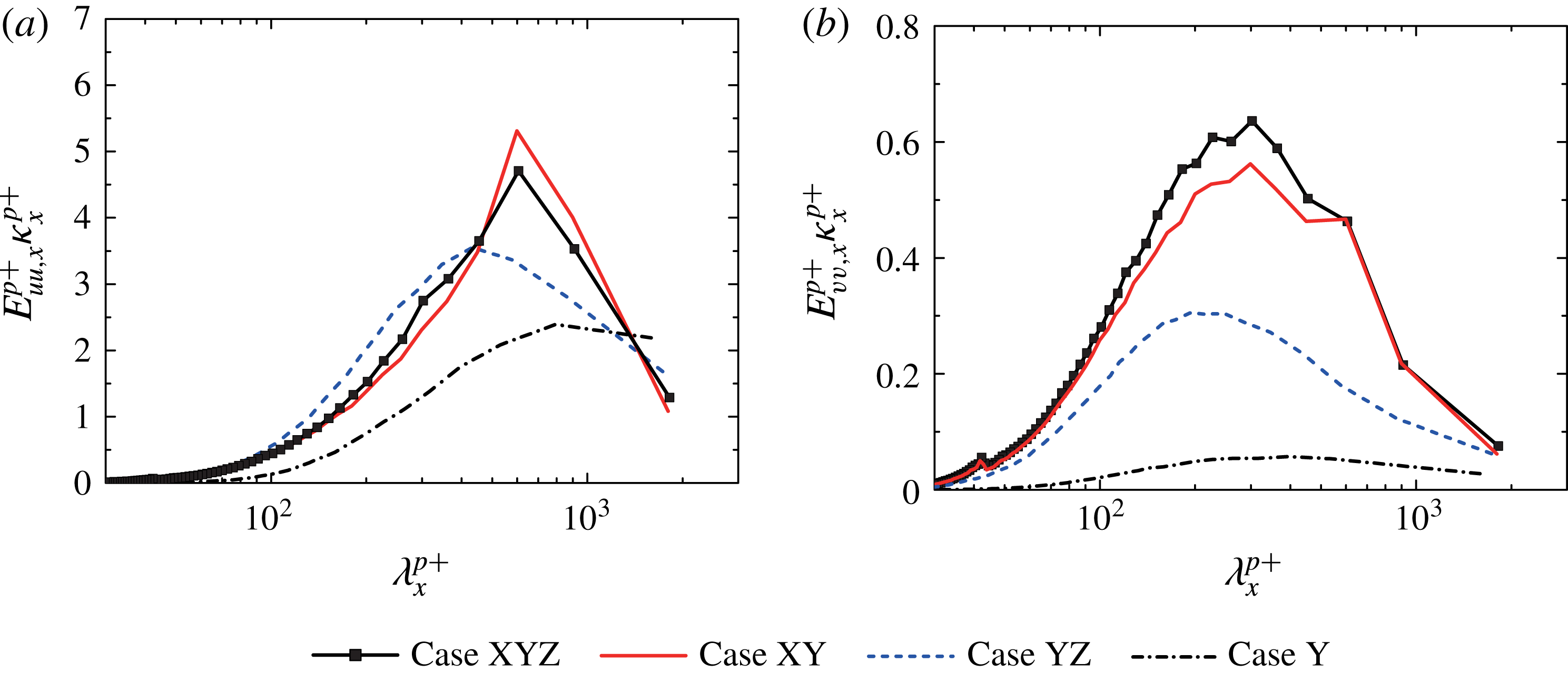
Figures 12 and 13 give the premultiplied streamwise and spanwise energy spectra, respectively, over the porous walls at
 $y^{p+}\approx 13$
. At the wavelength of
 $\unicode[STIX]{x1D706}_{x}^{p+}=600$
, a pointed profile of
 $E_{uu,x}$
and
 $E_{vv,x}$
in cases XY and XYZ can be seen in figure 13, which roughly corresponds to the wavelength of the streamwise large-scale perturbation by the KH instability estimated by the two-point correlations in figure 10. Furthermore,
 $E_{uu,x}$
has a maximum value at
 $\unicode[STIX]{x1D706}_{x}^{p+}=600$
, which means that streamwise velocity fluctuations in cases XY and XYZ are dominated by the large-scale perturbation. Moreover, it is also found from figure 13 that, in cases XY and XYZ, the spanwise spectra of
 $E_{uu,z}$
and
 $E_{vv,z}$
in the relatively long-wavelength region of
 $\unicode[STIX]{x1D706}_{z}^{p+}>300$
become far larger than those in cases Y and YZ. In figure 13, it is confirmed that the streamwise velocity fluctuations in cases Y and YZ are dominated by the coherent streaks of
 $\unicode[STIX]{x1D706}_{z}^{p+}\approx 100$
. Since the streaky structures are less organized in case YZ as observed in figure 7, which is also confirmed by the spanwise correlation of the streamwise velocity fluctuation in figure 11,
 $E_{uu,z}$
in case YZ loses energy at
 $\unicode[STIX]{x1D706}_{z}^{p+}\approx 100$
compared with that in case Y whilst
 $E_{uu,z}$
of longer-wavelength regions
 $\unicode[STIX]{x1D706}_{z}^{p+}>100$
in case YZ increases. Because the streamwise elongated streaks are no longer developed in cases XY and XYZ as observed in figure 7,
 $E_{uu,z}$
at
 $\unicode[STIX]{x1D706}_{z}^{p+}\approx 100$
in cases XY and XYZ is far smaller than that in case Y. Moreover, in figure 12(a),
 $E_{uu,x}$
in cases XY and XYZ becomes smaller in the long-wavelength region of
 $\unicode[STIX]{x1D706}_{x}^{p+}\approx 1500\sim 2000$
compared with those in cases Y and YZ. From these results, it is summarized that the large-scale streamwise perturbation developed over the streamwise permeable walls in cases XY and XYZ substantially contributes to the increase of
 $R_{11}$
and
 $R_{22}$
. However, owing to the reduction of the streaks in cases XY and XYZ, the enhancement of
 $R_{11}$
is less prominent compared with that of
 $R_{22}$
, as shown in figure 4. Note that, since the wavelength of the small kinks of
 $E_{vv,x}$
and
 $E_{vv,z}$
at
 $\unicode[STIX]{x1D706}_{x}^{p+}\approx 45$
in figures 12(b) and 13(b) corresponds to the pitch of the holes
 $D_{2}^{p+}=45$
, it is considered to be associated with the printed pattern of the porous walls, which can also be observed in figure 7. However, since the kink is negligibly small, the printed pattern fluctuations in figure 7 is found to hardly contribute to the enhancement of
 $R_{22}$
. When the pore size is further reduced, the influence of the printed pattern fluctuations becomes negligible.
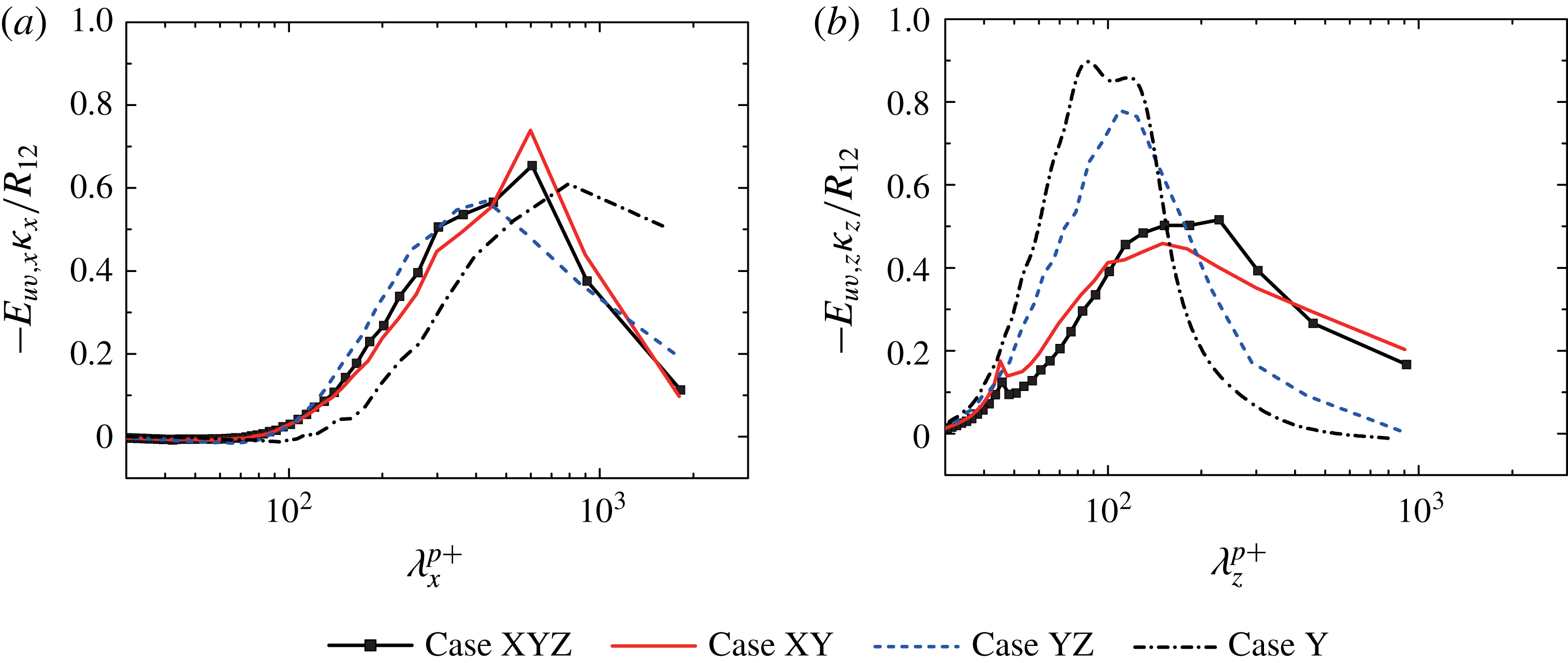
To clarify the contribution of the large-scale streamwise perturbation to the plane-averaged Reynolds shear stress, the premultiplied cospectrum of
 $E_{uv,x}$
and
 $E_{uv,z}$
normalized by
 $R_{12}$
is given in figure 14. From the streamwise cospectrum of
 $E_{uv,x}$
in figure 14(a), the contribution of the fluctuations in long-wavelength regions of
 $\unicode[STIX]{x1D706}_{x}^{p+}>800$
to
 $R_{12}$
in cases YZ, XY and XYZ becomes smaller compared with that in case Y whereas the contribution increases in the wavelength of
 $\unicode[STIX]{x1D706}_{x}^{p+}<500$
. Moreover, the profile of
 $E_{uv,x}$
in cases XYZ and XY exhibits a pointed peak at
 $\unicode[STIX]{x1D706}_{x}^{p+}=600$
. This means that, over the porous wall with the streamwise permeability, the large-scale streamwise perturbation contributes to
 $R_{12}$
, leading to the increase of friction. From the spanwise cospectrum of
 $E_{uv,z}$
in figure 14(b), it is found that
 $R_{12}$
in cases Y and YZ are dominated by fluctuations associated with streaks near
 $\unicode[STIX]{x1D706}_{z}^{p+}\approx 100$
whereas the locations of the global maximum in cases XY and XYZ shift to the longer-wavelength regions of
 $\unicode[STIX]{x1D706}_{z}^{p+}\approx 200$
. Although there are small kinks of
 $E_{uv,z}$
in cases XY and XYZ at wavelength of
 $\unicode[STIX]{x1D706}_{z}^{p+}\approx 45$
, which are associated with the printed pattern fluctuations in figure 7, the contribution to
 $R_{12}$
is found to be marginal.
Premultiplied cospectra normalized by
 $R_{12}$
: (a) streamwise cospectra
 $E_{uv,x}$
and (b) spanwise cospectra
 $E_{uv,z}$

4.5 Reynolds-number dependence
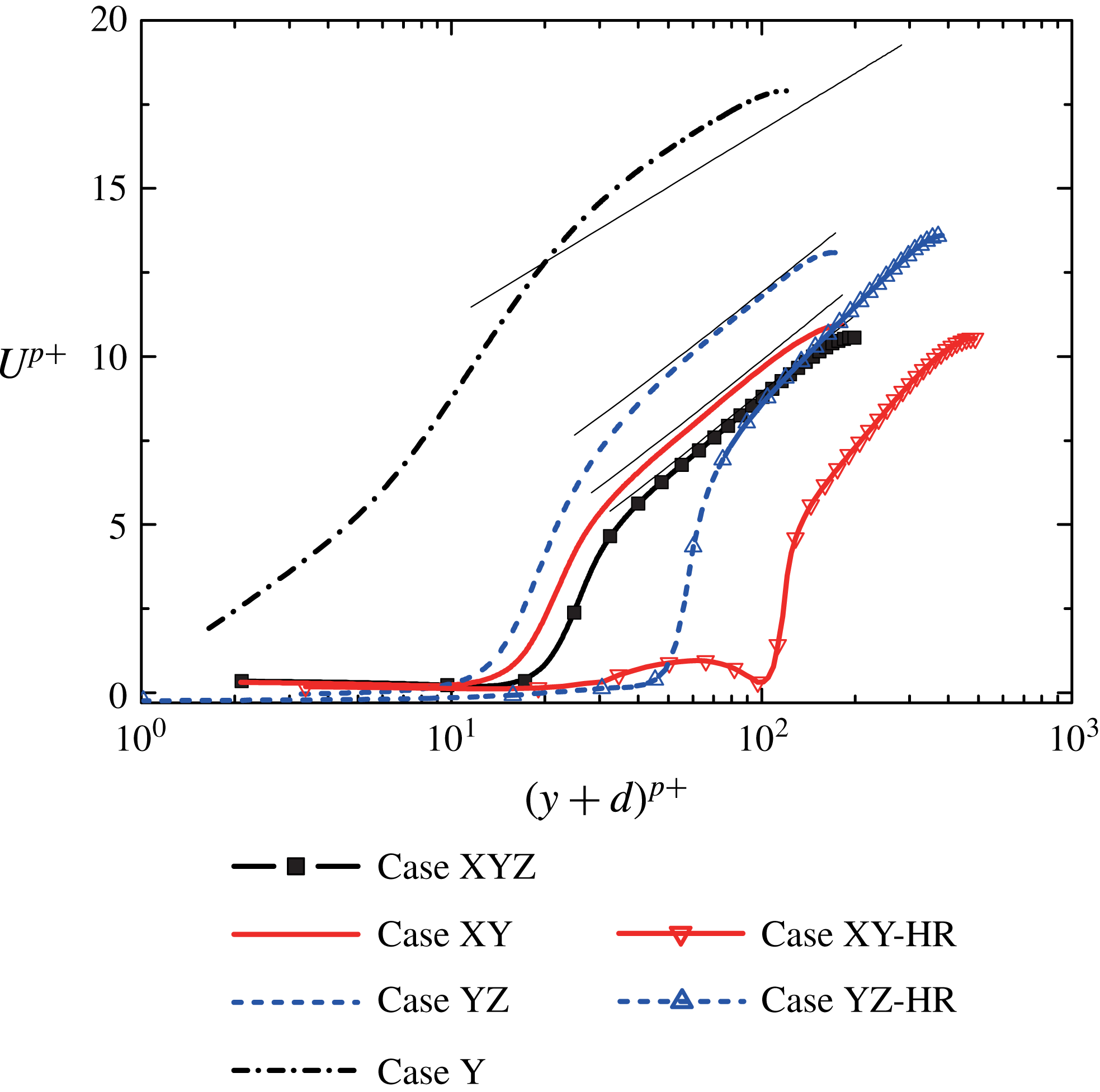
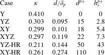
In order to discuss the characteristics of the streamwise mean velocity profiles in the semi-logarithmic scale of figure 15, the logarithmic velocity profile is considered as
 $$\begin{eqnarray}\overline{u}^{p+}=\frac{1}{\unicode[STIX]{x1D705}}\ln \left\{\frac{(y+d)^{p+}}{h_{r}^{p+}}\right\},\end{eqnarray}$$
where parameters
 $\unicode[STIX]{x1D705}$
,
 $d$
and
 $h_{r}$
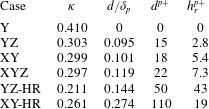
are, respectively, the Kármán constant, the zero-plane displacement and the equivalent roughness height, which are listed in table 6. (See Breugem et al. (Reference Breugem, Boersma and Uittenbogaard2006) or Suga et al. (Reference Suga, Matsumura, Ashitaka, Tominaga and Kaneda2010) for the procedure to obtain the parameters.) Distinct logarithmic profiles cannot be observed in case Y; however, since the mean velocity profile in case Y is almost symmetrical, as shown in figure 2, the value of
 $\unicode[STIX]{x1D705}$
is assumed to be the standard value of
 $\unicode[STIX]{x1D705}=0.41$
, and the values of
 $d$
and
 $h_{r}$
are assumed to be
 $d=0$
and
 $h_{r}=0$
. As the wall shear stress of the porous wall
 $\unicode[STIX]{x1D70F}_{w}^{p}/\unicode[STIX]{x1D70F}_{w}^{t}$
increases as seen in table 5, the profile shifts downwards from the standard log-law line. Furthermore, both the zero-plane displacement
 $d$
and the equivalent roughness height
 $h_{r}$
increase whilst the Kármán constant decreases as
 $\unicode[STIX]{x1D70F}_{w}^{p}/\unicode[STIX]{x1D70F}_{w}^{t}$
increases. Through the comparison between the different Reynolds-number cases XY and XY-HR or cases YZ and YZ-HR, it is found that, as the Reynolds number increases, the profile shifts rightwards and both
 $d$
and
 $h_{r}$
increase whilst
 $\unicode[STIX]{x1D705}$
decreases.
Streamwise mean velocity profiles with porous-wall scaling.

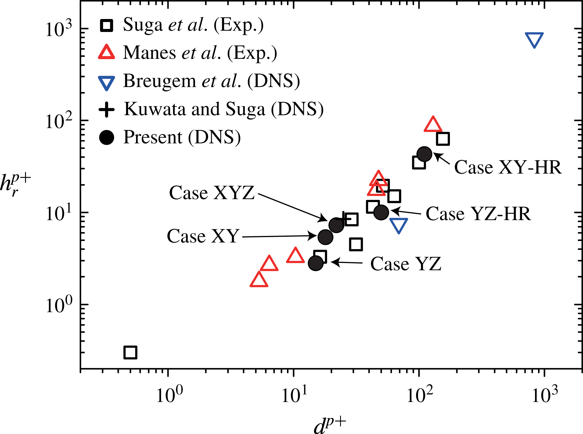
Zero-plane displacement versus the roughness height.

Characteristic parameters of the streamwise mean velocity: Kármán constant, zero-plane displacement and roughness height.
To compare those values with the previous experimental data of Manes et al. (Reference Manes, Pokrajac, McEwan and Nikora2009) and Suga et al. (Reference Suga, Matsumura, Ashitaka, Tominaga and Kaneda2010) and the DNS data of Breugem et al. (Reference Breugem, Boersma and Uittenbogaard2006) and Kuwata & Suga (Reference Kuwata and Suga2016b
), figure 16 plots
 $d^{p+}$
versus
 $h_{r}^{p+}$
. From figure 16, it is understood that, although the presently focused porous media have strong anisotropy and the structures are totally different from those considered in the experimental and DNS studies, there is a clear correlation between
 $d^{p+}$
and
 $h_{r}^{p+}$
. This result supports the discussions by Suga et al. (Reference Suga, Matsumura, Ashitaka, Tominaga and Kaneda2010) and Manes et al. (Reference Manes, Poggi and Ridolfi2011) that the increase of
 $d^{p+}$
and
 $h_{r}^{p+}$
can both be attributed to relaxation of wall blocking. It was reported by Suga et al. (Reference Suga, Matsumura, Ashitaka, Tominaga and Kaneda2010) and Manes et al. (Reference Manes, Poggi and Ridolfi2011) that the trend of
 $d^{p+}$
and
 $h_{r}^{p+}$
could be well characterized by the permeability Reynolds number
 $Re_{K}$
. However, since the streamwise permeability Reynolds number
 $Re_{Kx}$
in table 5 becomes zero in cases YZ and YZ-HR despite the fact that
 $d^{p+}\neq 0$
and
 $h_{r}^{p+}\neq 0$
, the streamwise permeability Reynolds number cannot be used as
 $Re_{K}$
straightforwardly. The wall-normal and spanwise permeabilities also need considering to represent the relaxation of the wall-blocking effect.
Figure 17 plots
 $\unicode[STIX]{x1D705}$
versus
 $d/\unicode[STIX]{x1D6FF}_{p}$
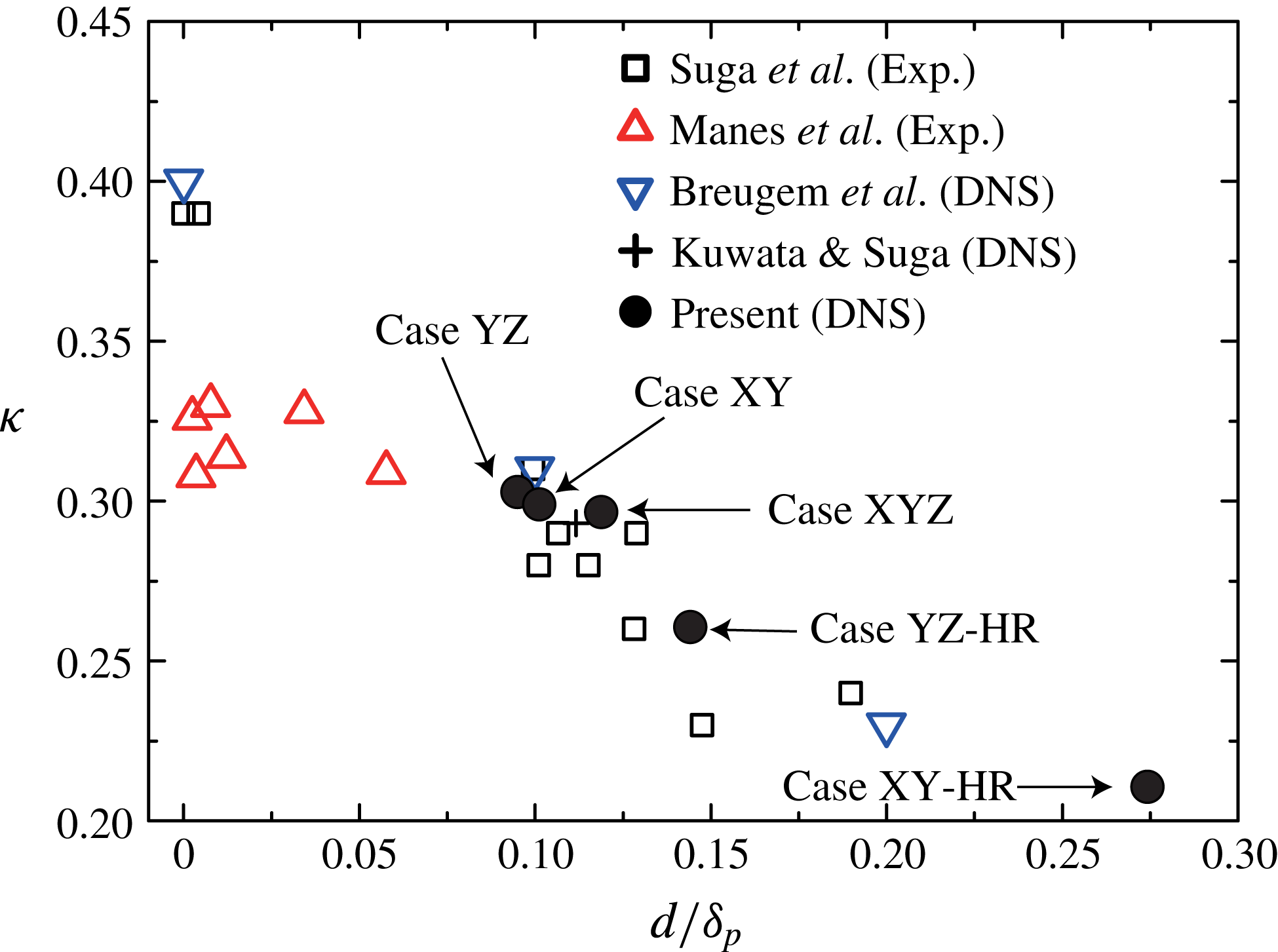
. Although Kármán constants in the range of smaller
 $d/\unicode[STIX]{x1D6FF}_{p}$
cases (
 $d/\unicode[STIX]{x1D6FF}_{p}<0.025$
) by Manes et al. (Reference Manes, Pokrajac, McEwan and Nikora2009) exhibit lower values than those reported for smooth wall and lower-permeability walls (Breugem et al.
Reference Breugem, Boersma and Uittenbogaard2006; Suga et al.
Reference Suga, Matsumura, Ashitaka, Tominaga and Kaneda2010), the consistent trend can be confirmed among the data of present DNS and Breugem et al. (Reference Breugem, Boersma and Uittenbogaard2006), Suga et al. (Reference Suga, Matsumura, Ashitaka, Tominaga and Kaneda2010) and Kuwata & Suga (Reference Kuwata and Suga2016b
). In the range of
 $d/\unicode[STIX]{x1D6FF}_{p}<0.15$
, the Kármán constant proportionally decreases with increasing
 $d/\unicode[STIX]{x1D6FF}_{p}$
whereas the decreasing rate becomes smaller in the range of
 $d/\unicode[STIX]{x1D6FF}_{p}>0.15$
. The clear correlations between
 $\unicode[STIX]{x1D705}$
and
 $d/\unicode[STIX]{x1D6FF}_{p}$
observed in figure 17 support the discussions of Manes et al. (Reference Manes, Pokrajac, McEwan and Nikora2009) that the Kármán constant can be scaled by the ratio of the boundary-layer thickness and the zero-plane displacement, meaning the ratio of the inner and outer length scales. This was also supported by the DNS of impermeable rough-wall turbulence studied by Leonardi & Castro (Reference Leonardi and Castro2010).
Kármán constant distribution versus the ratio of the zero-plane displacement and the boundary-layer thickness of the porous side.

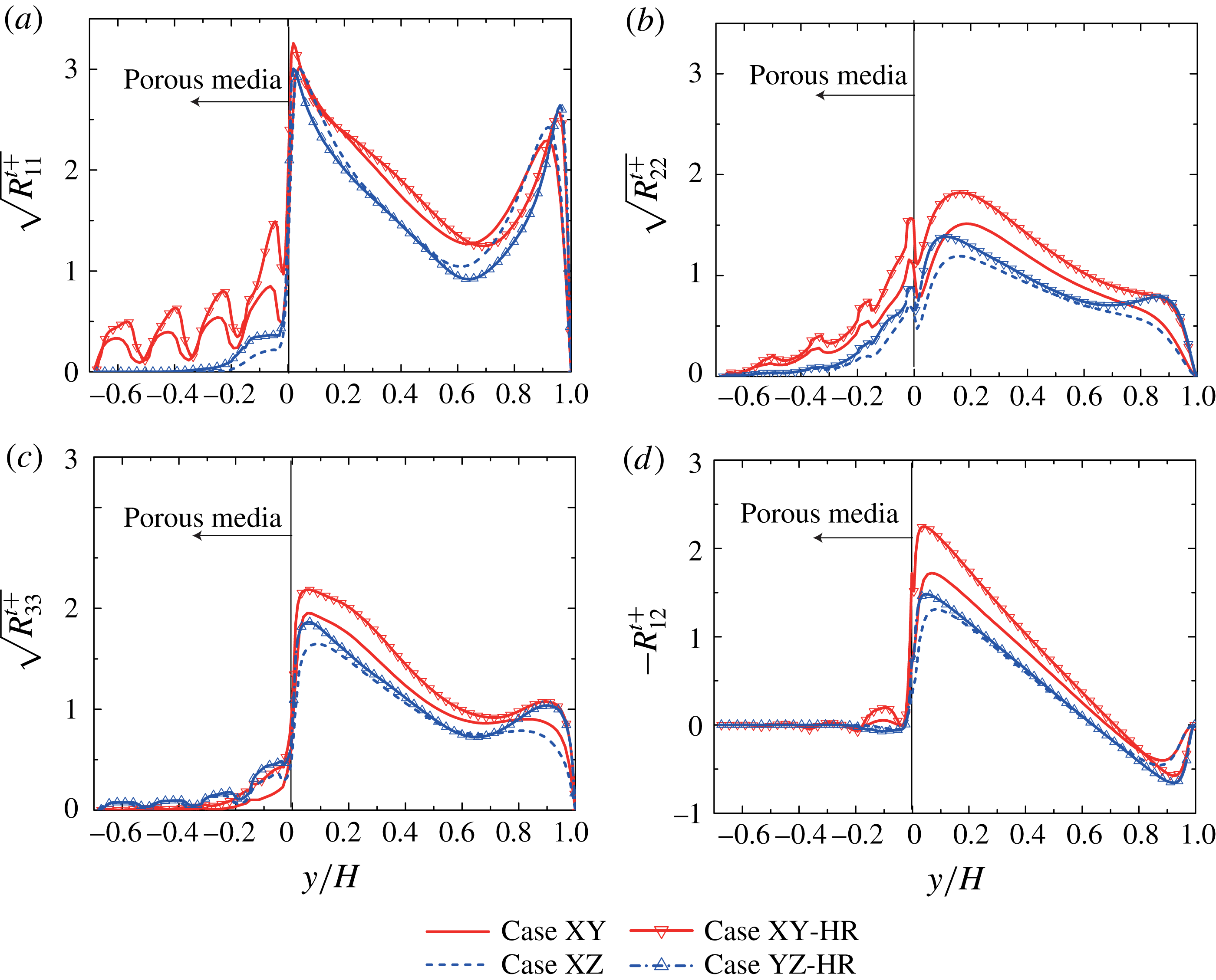
Figure 18 compares the plane-averaged Reynolds stresses normalized by
 $u_{\unicode[STIX]{x1D70F}}^{t}$
at different Reynolds numbers of
 $Re_{\unicode[STIX]{x1D70F}}=111$
and
 $230$
. As the Reynolds number increases, the plane-averaged Reynolds stresses of
 $R_{22}^{t+}$
,
 $R_{33}^{t+}$
and
 $R_{12}^{t+}$
increase substantially over the porous walls whilst
 $R_{11}^{t+}$
does not increase. It is found that the enhancement of
 $R_{12}$
due to the increase of
 $Re_{\unicode[STIX]{x1D70F}}$
in case XY is more remarkable than that in case YZ. Accordingly, as
 $Re_{\unicode[STIX]{x1D70F}}$
increases from
 $111$
to
 $230$
, the porous-wall shear stress in table 5 increases 5 % in case YZ and increases 21 % in case XY. This confirms that the Reynolds-number dependence is more remarkable in case XY than in case YZ. Inside the porous wall of
 $y/H<0$
, the plane-averaged Reynolds normal stresses are increased by the rise of
 $Re_{\unicode[STIX]{x1D70F}}$
; however, increase of the plane-averaged Reynolds shear stress is marginal. It rapidly converges to zero inside the porous wall even in the case of
 $Re_{\unicode[STIX]{x1D70F}}=230$
.
Plane-averaged Reynolds stresses at
 $Re_{\unicode[STIX]{x1D70F}}=111$
and
 $Re_{\unicode[STIX]{x1D70F}}=230$
normalized by
 $u_{\unicode[STIX]{x1D70F}}^{t}$
: (a) streamwise component, (b) wall-normal component, (c) spanwise component, and (d) off-diagonal component.

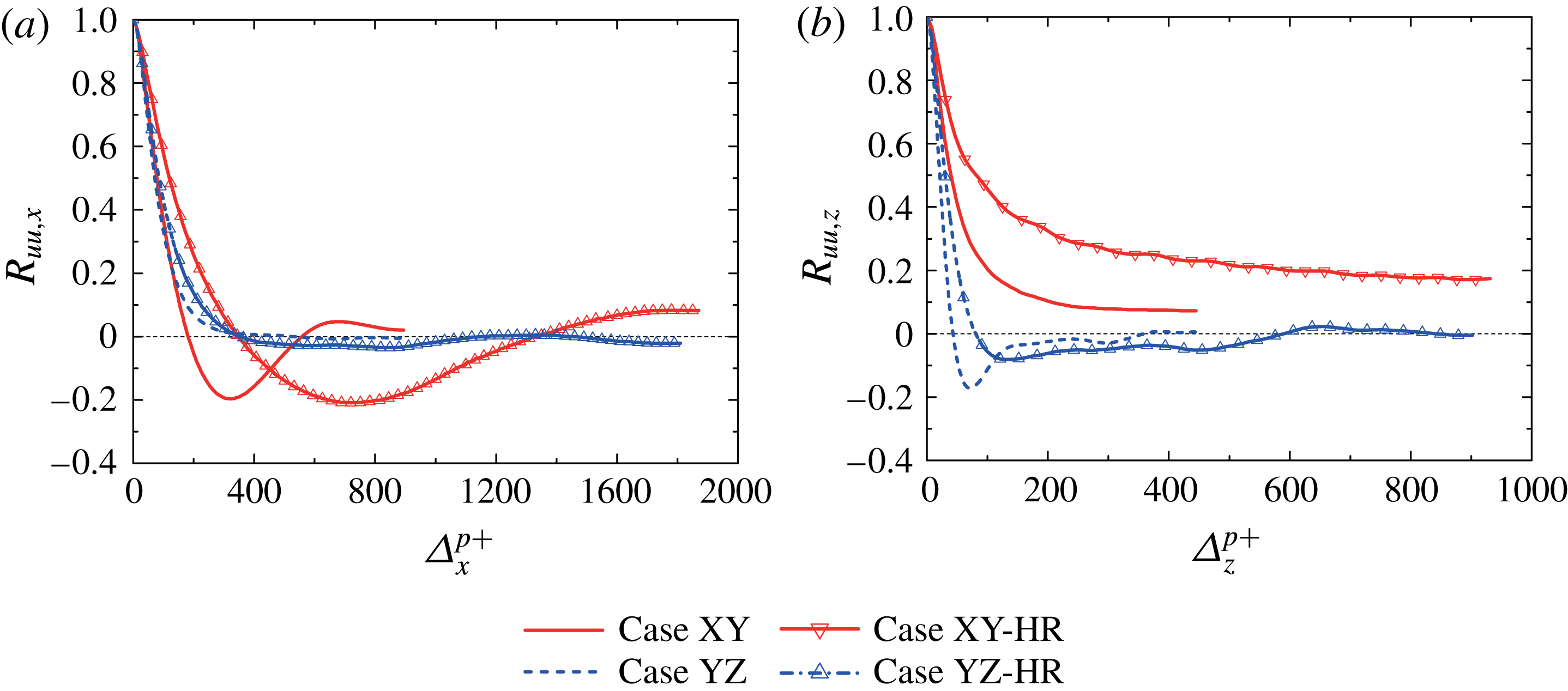
To investigate the Reynolds-number dependence of the large-scale streamwise perturbation, figure 19 compares the streamwise and spanwise two-point correlations of streamwise velocity fluctuations. As shown in figure 19(a), the streamwise correlation of
 $R_{uu,x}$
in case YZ-HR rapidly converges to zero whereas that in case XY-HR does not converge to zero and it shows a wavy profile. This indicates that, even for higher-Reynolds-number flows of
 $Re_{\unicode[STIX]{x1D70F}}=230$
, the streamwise perturbation does not develop over the spanwise permeable wall but develops over the streamwise permeable wall. The location of the local minimum shifts from
 $\unicode[STIX]{x1D6E5}_{x}^{p+}=300$
in case XY to
 $\unicode[STIX]{x1D6E5}_{x}^{p+}=700$
corresponding to the wavelength of
 $\unicode[STIX]{x1D706}_{x}^{p+}=1400$
. The magnitude of the local minimum value in case XY-HR at
 $\unicode[STIX]{x1D6E5}_{x}^{p+}=700$
is slightly larger than that at
 $\unicode[STIX]{x1D6E5}_{x}^{p+}=300$
in case XY. Moreover, it is also clear from figure 19(b) that, since the convergence of
 $R_{uu,z}$
in case XY-HR becomes slower compared with that in case XY, the stronger spanwise coherence is present across the full box. These results mean that, over the streamwise permeable wall, as the friction Reynolds number increases from
 $111$
to
 $230$
, the wavelength of the streamwise perturbation increases from
 $\unicode[STIX]{x1D706}_{x}^{p+}=600$
to
 $\unicode[STIX]{x1D706}_{x}^{p+}=1400$
and the perturbation becomes more organized.
Two-point correlations of the streamwise velocity fluctuations at
 $Re_{\unicode[STIX]{x1D70F}}=111$
and
 $Re_{\unicode[STIX]{x1D70F}}=230$
: (a) streamwise correlation and (b) spanwise correlation.

This kind of large-scale coherent eddy motion is also observed near vegetated canopy flows. Raupach et al. (Reference Raupach, Finnigan and Brunei1996) and Finnigan (Reference Finnigan2000) summarized that the wavelength of this large-scale eddy motion
 $\unicode[STIX]{x1D706}_{x}$
was proportional to the vorticity thickness
 $\unicode[STIX]{x1D6FF}_{\unicode[STIX]{x1D714}}$
as
 $\unicode[STIX]{x1D706}_{x}=C_{\unicode[STIX]{x1D706}}\unicode[STIX]{x1D6FF}_{\unicode[STIX]{x1D714}}$
. Here, the constant value of
 $C_{\unicode[STIX]{x1D706}}=4.05$
was the best fitted value in a wide range of canopy types. Since this value was in the range of the spacing of KH-type coherent eddies in the fully developed mixing layer,
 $3.5\leqq \unicode[STIX]{x1D706}_{x}/\unicode[STIX]{x1D6FF}_{\unicode[STIX]{x1D714}}\leqq 5$
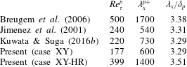
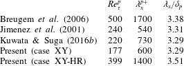
(Dimotakis & Brown Reference Dimotakis and Brown1976; Rogers & Moser Reference Rogers and Moser1994), it was evident that turbulent flows over a canopy behaved as a plane mixing layer rather than a boundary layer. To discuss the length scale of the streamwise perturbation over porous media, table 7 summarizes the wavelength of the perturbation in cases XY and XY-HR and other data in the literature of flows over porous walls (Jimenez et al.
Reference Jimenez, Uhlmann, Pinelli and Kawahara2001; Breugem et al.
Reference Breugem, Boersma and Uittenbogaard2006; Kuwata & Suga Reference Kuwata and Suga2016b
). In terms of porous-wall turbulence, it is clear that no meaningful tendency can be observed by the normalization of the inner scale whereas the wavelength normalized by the outer layer scale such as the boundary-layer thickness
 $\unicode[STIX]{x1D706}_{x}/\unicode[STIX]{x1D6FF}_{p}$
coincides with
 $\unicode[STIX]{x1D706}_{x}/\unicode[STIX]{x1D6FF}_{p}\approx 3.4$
, despite the fact that the flow conditions and the porous-medium characteristics (such as porosity, permeability and Forchheimer tensors) focused in those studies are entirely different. Supposing that the boundary-layer thickness
 $\unicode[STIX]{x1D6FF}_{p}$
represents the vorticity thickness
 $\unicode[STIX]{x1D6FF}_{\unicode[STIX]{x1D714}}$
over the porous walls, the constant value of the relation
 $\unicode[STIX]{x1D706}_{x}=C_{\unicode[STIX]{x1D706}}\unicode[STIX]{x1D6FF}_{\unicode[STIX]{x1D714}}$
becomes
 $C_{\unicode[STIX]{x1D706}}=3.4$
, which is close to the value obtained in canopy flows (
 $C_{\unicode[STIX]{x1D706}}=4.05$
) and the fully developed mixing layer (
 $3.5\leqq C_{\unicode[STIX]{x1D706}}\leqq 5$
). This result implies that the mechanism of the generation of the streamwise perturbation is the same as that in the fully developed mixing layer. Moreover, it is interesting to stress that the wavelength of the streamwise perturbation does not depend on the porous-medium characteristics.
Streamwise wavelength of the large-scale streamwise perturbation.
To examine the coherence of the streamwise perturbation, the magnitude of the local minimum value of R
 $_{uu,x}$
is examined. It is expected that, as the streamwise wall permeability decreases (the viscous drag increases), large-scale turbulence motion penetrated into the porous walls tend to be blocked and dissipated. Consequently, the streamwise perturbation loses coherence. However, even though the streamwise permeability Reynolds number is almost the same in case XY-HR (
 $Re_{Kx}=10$
) and case E95 (
 $Re_{Kx}=9.35$
) of Breugem et al. (Reference Breugem, Boersma and Uittenbogaard2006), the magnitude of the local minimum value of
 $R_{uu,x}$
in case XY-HR shows
 $0.21$
whilst that in case E95 is less than 0.1. This discrepancy may be attributed to inertial effects. When the inertial effect, which is expressed as the Forchheimer drag term (second term on the right-hand side of (3.1)), becomes more significant, it is expected that turbulence penetration tends to be blocked and disturbance inside porous media tends to be rapidly decayed. Consequently, the large-scale perturbation loses coherence due to the inertial effects. Since the pore in case XY goes through along the streamwise direction, the inertial effect (streamwise Forchheimer drag) is less significant than for the porous medium of E95 in Breugem et al. (Reference Breugem, Boersma and Uittenbogaard2006). Indeed, the coherence is stronger over the porous media in case XY than that in case E95 of Breugem et al. (Reference Breugem, Boersma and Uittenbogaard2006). Hence, it is further expected that, over a porous wall with lower permeability and with higher Forchheimer number, such as geological rocks, the streamwise perturbation loses coherence and finally disappears.
5 Conclusion
To examine which component of the permeability tensor influences turbulence over porous walls, the direct numerical simulation of anisotropic porous-walled channel flows is performed by the D3Q27 multiple-relaxation-time lattice Boltzmann method with the imbalance correction zonal grid refinement method. The presently considered porous media are a wall with square pore arrays aligned with the Cartesian axes. Four kinds of anisotropic porous walls are made by systematically introducing pore arrays, namely walls with only vertical permeability, with vertical and streamwise permeabilities, with vertical and spanwise permeabilities, and with vertical, spanwise and streamwise permeabilities. Simulations are performed at the friction Reynolds number of 111 and 230.
It is found that turbulence is not altered by vertical permeability itself whilst streamwise and spanwise permeabilities considerably enhance the Reynolds stresses over the porous walls. The enhancement of the streamwise Reynolds stress is marginal; however, the spanwise and wall-normal Reynolds stresses and the Reynolds shear stress are substantially enhanced. It is revealed that enhancement of turbulence is more remarkable over porous media with streamwise permeability. It is confirmed through the comparison between the rough-wall and porous-wall simulations that the enhancement of turbulence over the porous wall in streamwise pores compared with that over the porous wall in spanwise pores is not due to the difference of the wall roughness, but due to difference in the wall permeability.
Since the porous wall with only vertical permeability almost behaves like a smooth solid wall, the elongated streaky structures that are usually observed over a smooth wall are also formed over the porous wall with only vertical permeability. However, they are twisted and shredded over the porous wall with spanwise permeability. Furthermore, over the porous wall with streamwise permeability, streaky structures no longer appear whereas the vortices are found to be shrunken by intermittent patched pattern ejections. Two-point correlation analysis suggests that streamwise permeability allows development of streamwise perturbation of the wavelength of 600 wall units induced by the Kelvin–Helmholtz instability. This causes the intermittent turbulence structures around the porous wall. Spectral analysis elucidates that this perturbation contributes to the enhancement of the plane-averaged Reynolds shear stress, leading to a significant rise in wall friction of the porous wall. However, it is also found that, since the development of the streaky structures is prevented by a strong wall-normal velocity disturbance, the enhancement of the streamwise component of the Reynolds normal stresses is less prominent.
The characteristic parameters of the streamwise mean velocity, such as the zero-plane displacement, the equivalent roughness height and the Kármán constant, are compared with the previous experimental and DNS studies. Although the geometric structures of the presently focused porous media are totally different from the isotropic porous media considered in the previous experimental and DNS studies, a consistent trend can be observed that the equivalent roughness height increases as the zero-plane displacement increases. Furthermore, it is confirmed that the Kármán constant can be well scaled by the ratio of the boundary-layer thickness and the zero-plane displacement, which represents the ratio of the inner and outer length scales. As the increase of the inner length scale becomes more significant compared with that of the outer length scale, the Kármán constant decreases.
Through a comparison of the plane-averaged Reynolds stresses for lower- and higher-Reynolds-number flows, it is clear that the maximum values of the streamwise Reynolds stress over the porous walls are almost the same, whereas the spanwise and wall-normal Reynolds stresses and the Reynolds shear stress increase with the increase of the Reynolds number. It is also found that the Reynolds-number dependence of the plane-averaged Reynolds stress over the wall with streamwise permeability is more obvious than that over the wall with spanwise permeability. Indeed, when the friction Reynolds number increases from
 $111$
to
 $230$
, the wall shear stresses over the porous wall with streamwise and spanwise permeabilities increase
 $21\,\%$
and
 $5\,\%$
, respectively. The two-point correlation analysis reveals that, when the friction Reynolds number increases from
 $111$
to
 $230$
, the wavelength of the streamwise perturbation over the porous wall with streamwise permeability increases from
 $600$
to
 $1400$
porous-wall units. The wavelength of the large-scale perturbation is found to be proportional to the outer-layer scale rather than the inner-layer scale irrespective of the difference of the porous-medium characteristics and flow conditions. Assuming that the boundary-layer thickness over the porous wall can represent the vorticity thickness of the large-scale motion, the ratio of the wavelength of the streamwise perturbation and the vorticity thickness over the porous wall is close to that in the fully developed mixing layer. This suggests that the generation process of large coherent structures over the porous wall is similar to that in the plane mixing layer.
Concerned with the coherence of the streamwise perturbation, it should be stressed that the coherence of the large-scale motion is significantly influenced by the permeability and Forchheimer tensors, even though the length scale of the streamwise perturbation is insensitive to the porous characteristics. For porous media with large tortuosity or low porosity, the wall permeability decreases and the Forchheimer drag increases. Consequently, the perturbation may be dissipated and lose coherence in this kind of porous media.
Acknowledgements
The authors express their gratitude to their colleagues, Dr M. Kaneda and Professor Y. Kawaguchi, for their support. A part of this study was financially supported by the research grant (no. 26.10154) of the JSPS Japan. The numerical calculations were carried out on the TSUBAME 2.5 supercomputer in Tokyo Institute of Technology in a research project (ID: jh160042-NAH) of the JHPCN.
Appendix. Comparison with the experimental data
To validate the present DNS results, simulated plane-averaged mean velocity and Reynolds stress profiles are compared with the experimental data of Suga et al. (Reference Suga, Matsumura, Ashitaka, Tominaga and Kaneda2010). Considering the bulk mean Reynolds number and the porous-wall friction Reynolds number, the experimental data of no. 13 at
 $Re_{b}=2600$
(
 $Re_{\unicode[STIX]{x1D70F}}^{p}=153$
) and no. 06 at
 $Re_{b}=2800$
(
 $Re_{\unicode[STIX]{x1D70F}}^{p}=225$
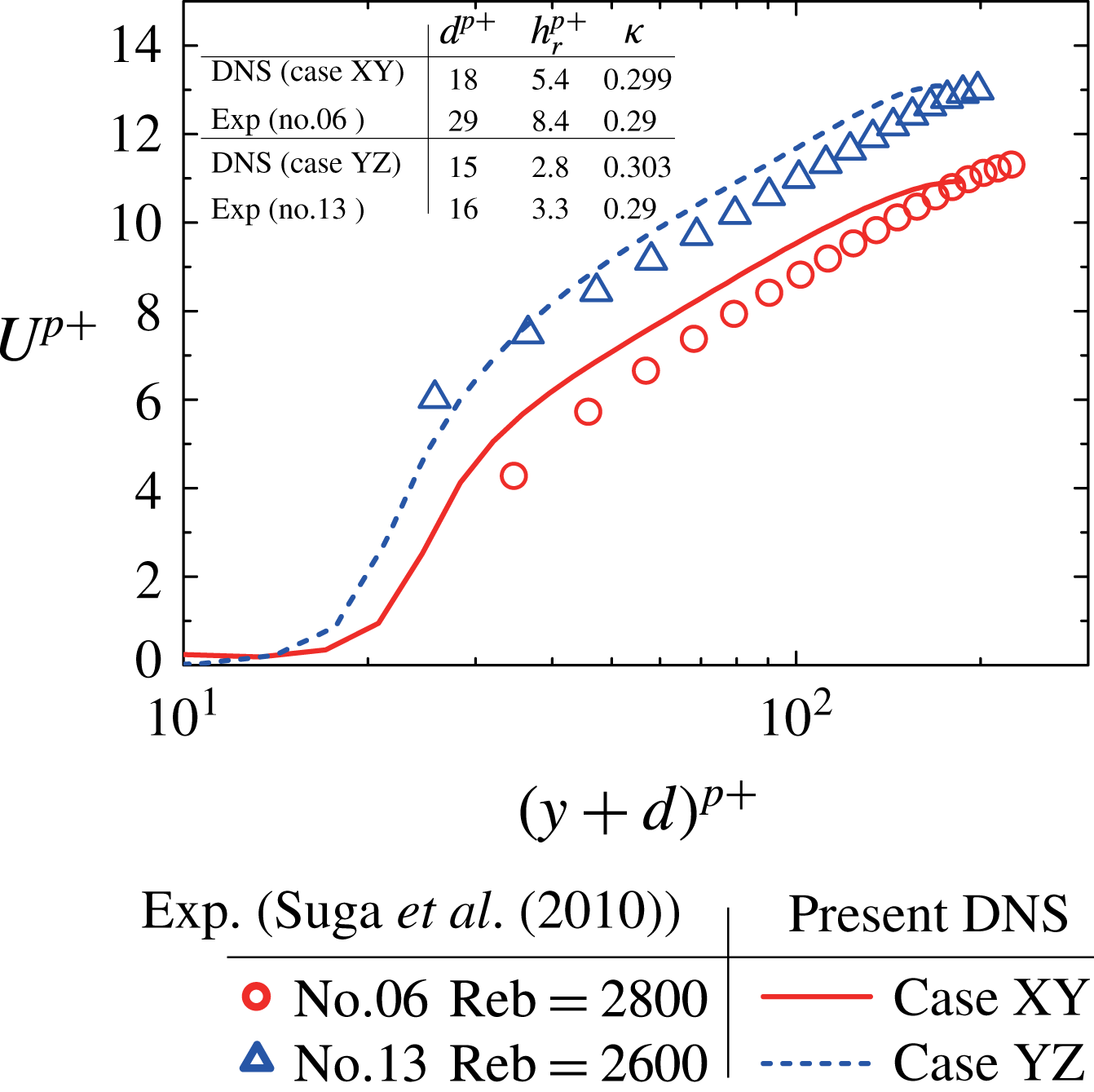
) are selected as comparable cases for YZ and XY, respectively. Figure 20 compares the streamwise mean velocity normalized by
 $u_{\unicode[STIX]{x1D70F}}^{p}$
with porous-wall scaling of (4.2). The zero-plane displacement, the equivalent roughness height and the Kármán constant are also included in figure 20. Corresponding to increase of skin friction over the porous walls, both simulated and experimental streamwise mean velocity profiles shift downwards. However, the downward shifts are slightly underpredicted, and, besides, the predicted profiles shift to the left compared with the experimental data. Accordingly, both
 $d^{p+}$
and
 $h_{r}^{p+}$
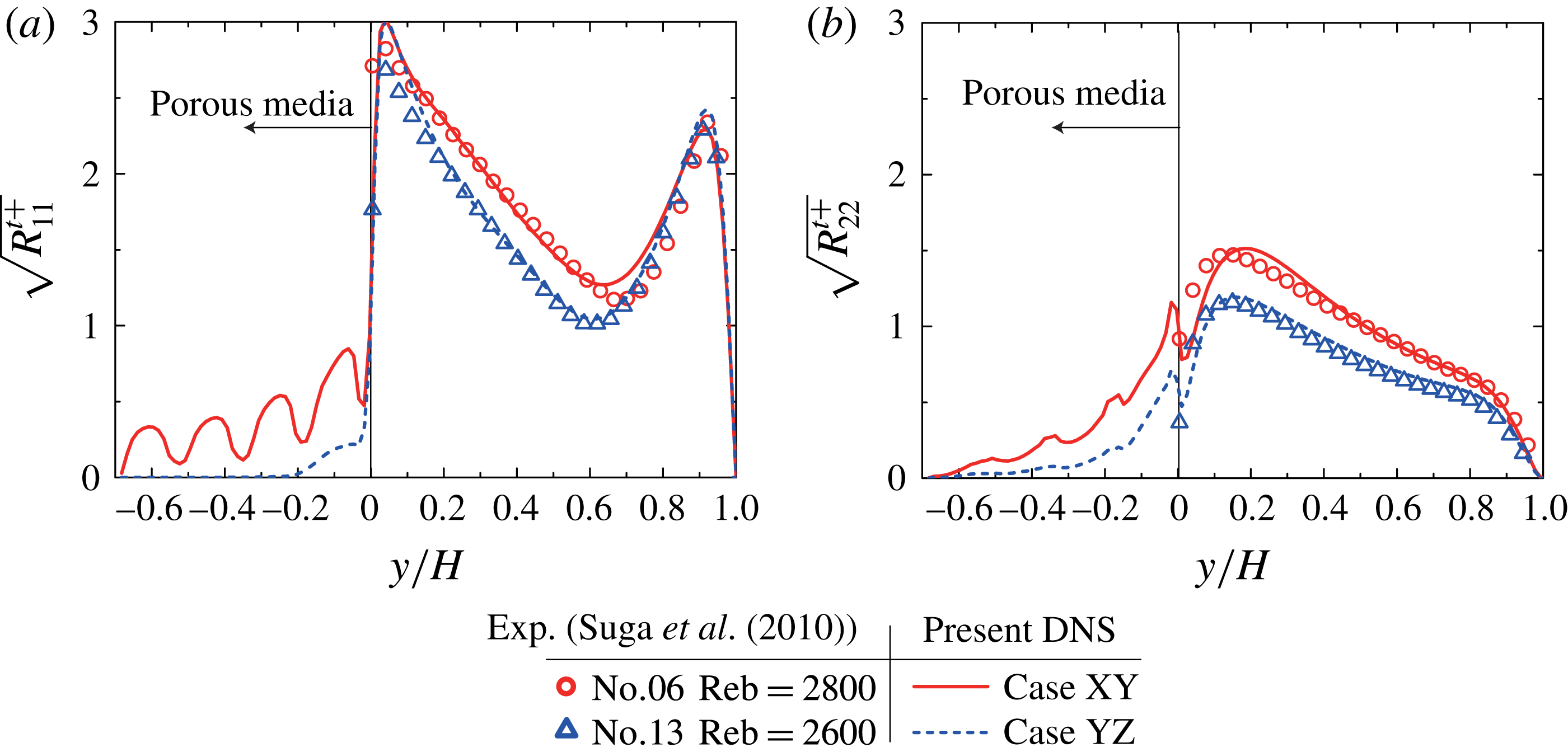
are slightly underpredicted. On the other hand, since the slope of the profiles in log-law regions agrees well with the experimental data, the Kármán constants of the simulated profiles correspond well to the experimental data. Figure 21 compares the plane-averaged Reynolds stress profiles normalized by
 $u_{\unicode[STIX]{x1D70F}}^{t}$
. It is also confirmed in figure 21(b) that the enhancement of the wall-normal Reynolds stress near the porous wall in the experimental data is very well captured by the present DNS. Furthermore, overall agreement of the streamwise Reynolds stress between the experimental data and the predicted results in 21(a) can also be confirmed.
Comparisons of the plane-averaged streamwise mean velocity with porous-wall scaling between the experimental data of Suga et al. (Reference Suga, Matsumura, Ashitaka, Tominaga and Kaneda2010) and the present DNS.

Comparisons of the plane-averaged Reynolds stresses normalized by
 $u_{\unicode[STIX]{x1D70F}}^{t}$
between the experimental data of Suga et al. (Reference Suga, Matsumura, Ashitaka, Tominaga and Kaneda2010) and the present DNS: (a)
 $R_{11}^{t+}$
and (b)
 $R_{22}^{t+}$
.