





1. Introduction
Modern electrical devices often demand efficient cooling systems to dissipate heat and maintain optimal operating conditions (Zhang et al. Reference Zhang, Wang and Yan2021). For example, driven by significant progress in lithography and advanced packaging, the typical heat generated by modern high-performance electronics requires cooling heat fluxes exceeding
 $10^3\ \mathrm{W\,cm^{-2}}$
(Wu & Wang Reference Wu and Wang2025). The present primary cooling system remains air based, but the next generation focuses on fluid-flow-based systems, underscoring the importance of hydrodynamics in contemporary thermal management (Konovalov et al. Reference Konovalov, Tolstorebrov, Eikevik, Kobalava, Radchenko, Hafner and Radchenko2023; Wu & Wang Reference Wu and Wang2025).
In many practical cooling configurations, a working fluid passes through a channel where one wall is heated and the opposite wall is much cooler, producing a thermally stratified layer. A canonical framework that captures this interplay of forced and buoyancy-driven motions is the Rayleigh–Bénard–Poiseuille (RBP) flow, in which a pressure-driven stream in a horizontal channel is subjected to a transverse temperature gradient. Instabilities in this configuration manifest through two primary pathways: shear mechanisms dependent on the Reynolds number
 $\textit{Re}$
that provoke Tollmien–Schlichting waves (Schmid & Henningson Reference Schmid and Henningson2001), and buoyancy-driven modes governed by the Rayleigh number
 $Ra$
or the Richardson number
 $\textit{Ri}$
that result in the formation of convective rolls (Kelly Reference Kelly1994; Nicolas Reference Nicolas2002). However, in many practical applications, such as microchannels in solar units or electronic cooling chips (Sharma et al. Reference Sharma, Tiwari, Zimmermann, Brunschwiler, Schlottig, Michel and Poulikakos2015; Khalili et al. Reference Khalili, Sheikholeslami and Momayez2023),
 $\textit{Re}$
typically remains of
 $\mathcal{O}(10^2)$
, a regime where only buoyancy instability is triggered. Consequently, leveraging buoyancy instability to optimise thermal performance has become an active area of research. Taher & Abid (Reference Taher and Abid2018) experimentally demonstrated that buoyancy-induced secondary flows significantly enhance heat transfer compared with pure forced convection. Expanding on this work, Taher et al. (Reference Taher, Ahmed, Haddad and Abid2021) combined experiments with simulations to provide a detailed map of flow pattern evolution throughout the entire channel: from the entrance to the later turbulent regions. Furthermore, Zhang et al. (Reference Zhang, Huang, Peng and Li2023) employed three-dimensional numerical simulations to investigate how Rayleigh number
 $Ra$
, Reynolds number
 $\textit{Re}$
and lateral confinement affect the stability limits and transitions between longitudinal and transverse-roll structures in mixed convection. Beyond passive mechanisms, active control strategies to further increase heat transfer in RBP flows (Yan et al. Reference Yan, Wu, Gao and Li2023, Reference Yan, Gao, Zheng, Wu, Zheng and Ding2026) have also been investigated. However, continued miniaturisation reduces channel dimensions and hence the Rayleigh number, which scales with the cube of the channel height. In microscale channels,
 $Ra$
can therefore fall below the critical threshold for buoyancy-driven instability, leaving the flow laminar and eliminating buoyancy-induced mixing.
One potential strategy to overcome this suppression of instability and hence mixing is the addition of long-chain polymers to the working fluid. The stretching and relaxation of these polymer chains give rise to elastic stresses, which can fundamentally modify flow stability (Steinberg Reference Steinberg2021; Datta et al. Reference Datta2022; Dubief et al. Reference Dubief, Terrapon and Hof2023). In channels featuring curved geometries, such as wavy or serpentine paths or those containing internal obstacles, the well-known hoop stress polymer instability can lead to elastic turbulence (Groisman & Steinberg Reference Groisman and Steinberg2000). To date, the literature on elasticity-induced heat-transfer enhancement (HTE) has largely focused on this phenomenon. For instance, Abed et al. (Reference Abed, Whalley, Dennis and Poole2016) experimentally observed that heat transfer increased by up to 200 % for low polymer concentrations and up to 380 % for higher concentrations compared with equivalent Newtonian flows in a serpentine channel. Similarly, Roy et al. (Reference Roy, Taylor and Poulikakos2024) numerically demonstrated that heat transfer can reach approximately twice that of its Newtonian counterpart in channels with obstacles. Other experimental (Traore et al. Reference Traore, Castelain and Burghelea2015; Whalley et al. Reference Whalley, Abed, Dennis and Poole2015; Yang et al. Reference Yang, Yao and Wen2020) and numerical (Li et al. Reference Li, Zhang, Cheng, Li, Li, Qian and Joo2017; Garg & Wang Reference Garg and Wang2024) studies have confirmed this HTE phenomenon induced by elastic turbulence.
Conversely, in straight-channel flows, some studies have reported a reduction in heat transfer in Rayleigh–Bénard convection (Cai et al. Reference Cai, Wei, Tang, Liu, Li and Li2019; Xu et al. Reference Xu, Zhang, Brandt, Song and Shishkina2025), whereas others have observed both enhancement and suppression, with the reported enhancement remaining modest (e.g. approximately 2 % in Wang et al. Reference Wang, Cheng, Zhang, Zheng, Cai and Siginer2023 and approximately 10 % in Dubief & Terrapon Reference Dubief and Terrapon2020). Recently, it has been found that other viscoelastic instabilities, such as the centre mode (Khalid et al. Reference Khalid, Chaudhary, Garg, Shankar and Subramanian2021) and polymer diffusive instability (PDI) (Beneitez et al. Reference Beneitez, Page and Kerswell2023), can be triggered in a straight channel. However, the effectiveness of the resulting motions for heat flux has yet to be explored. This study represents a first attempt to address this issue, specifically focusing on cases where the centre mode is excited.
In this paper, we will conduct linear stability analysis and direct numerical simulations to investigate HTE in viscoelastic, unstably stratified (RBP flow) and stably stratified shear flow. To the best of our knowledge, previous studies have only focused on the stability analysis of similar systems, and the HTE effect has not been previously investigated in the literature as this requires a finite-amplitude manifestation of the instability to assess. An early investigation of viscoelastic RBP flow (Hirata et al. Reference Hirata, Alves, Delenda and Ouarzazi2015) focused on the convective and absolute instabilities by linear stability analysis, finding that, while fluid elasticity acts to stabilise transverse rolls in the presence of throughflow, it significantly accelerates the transition to absolute instability. Yao et al. (Reference Yao, Lu, Zhou, Luo, Yi and Tan2024) also conducted linear stability analysis and identified three distinct instability regimes governed by shear intensity (quantified by
 $\textit{Re}$
), revealing a non-monotonic dependence where viscoelasticity acts to destabilise the flow at low and high
 $\textit{Re}$
but plays a stabilising role at moderate
 $\textit{Re}$
. In contrast to these modal analyses, Yao et al. (Reference Yao, Lu, Zhang, Luo and Yi2025) focused on the linear non-modal dynamics of similar systems and uncovered a substantial transient energy growth driven by the coupling between polymeric stresses and temperature gradients. Furthermore, Kamboj et al. (Reference Kamboj, Patne, Narayana and Sahu2025) considered the effect of viscous heating, highlighting that the buoyancy induced by internal viscous dissipation can dramatically exacerbate purely elastic instabilities by lowering the critical Weissenberg number
 $W$
.
The rest of this paper is organised as follows. Section 2 formulates the physical problem and its governing equations. Section 3 is dedicated to linear stability analysis and a discussion of the fastest-growing modes. In § 4, we conduct the direct numerical simulations (DNS) to investigate the evolution of those unstable modes, including the numerical set-up (§ 4.1), a characterisation of representative flow cases (§ 4.2) and a parametric study of the Reynolds and Weissenberg numbers (§ 4.3). We then investigate the connection between the flow field and any HTE effects in § 4.4, and explore the self-sustaining mechanism of the nonlinear resulting states through a perturbation kinetic energy budget analysis in § 4.5. In § 5, we evaluate the thermal-hydraulic efficiency from an engineering perspective. Finally, concluding remarks are provided in § 6.
2. Problem formulation
2.1. Governing equations
Schematic of the Poiseuille channel flow.

We consider pressure-driven flow of an incompressible viscoelastic fluid in a channel with two walls at
 $z = \pm H$
, as shown in figure 1. The dimensionless continuity, Navier–Stokes, Oldroyd-B and density transport equations under the Boussinesq approximation can be written as
 \begin{align} \boldsymbol{\nabla }\boldsymbol{\cdot }\boldsymbol{u} = 0, \end{align}
 \begin{align} \frac {\partial \boldsymbol{u}}{\partial t} + \boldsymbol{u}\boldsymbol{\cdot }\boldsymbol{\nabla }\boldsymbol{u} = -\boldsymbol{\nabla }\!p + \frac {1-\beta }{\textit{Re}}\boldsymbol{\nabla }\boldsymbol{\cdot }\boldsymbol{\tau } + \frac {\beta }{\textit{Re}}{\nabla} ^2\boldsymbol{u} + Ri\rho \boldsymbol{\hat z} \, + \frac {2}{\textit{Re}}\boldsymbol{\hat x}, \end{align}
 \begin{align} \frac {{\partial {\boldsymbol{\tau }}}}{{\partial t}} + {\boldsymbol{u}} \boldsymbol{\cdot }\boldsymbol{\nabla }{\boldsymbol{\tau }} - {(\boldsymbol{\nabla }{\boldsymbol{u}})^{\textrm{T}}} \boldsymbol{\cdot }{\boldsymbol{\tau }} - {\boldsymbol{\tau }} \boldsymbol{\cdot }\boldsymbol{\nabla }{\boldsymbol{u}} + \frac {1}{{{W}{\mkern 1mu} }}{\boldsymbol{\tau }} = \frac {1}{{{W}{\mkern 1mu} }}\big [ {\boldsymbol{\nabla }{\boldsymbol{u}} + {{(\boldsymbol{\nabla }{\boldsymbol{u}})}^{\textrm{T}}}} \big ] + {\mkern 1mu} \frac {1}{{{\mathop {\textit{Re}}\nolimits } \textit{Sc}}} {\mkern 1mu} {{\nabla} ^2}{\boldsymbol{\tau }}, \end{align}
 \begin{align} {\mkern 1mu} \frac {{\partial \rho }}{{\partial t}} + {\boldsymbol{u}} \boldsymbol{\cdot }\boldsymbol{\nabla }\rho = \frac {1}{{{\textit{Pr}}{\mkern 1mu} {\textit{Re}}}}{{\nabla} ^2}\rho . \end{align}
These equations have been non-dimensionalised by the centreline speed of the base Poiseuille flow solution
 $U^*$
(see (2.9)), the half-height of the channel
 $H$
and the densities imposed at the isothermal walls (
 $\rho _{\textit{UW}}^*$
is the enforced density at the upper wall and
 $\rho _{\textit{LW}}^*$
at the lower wall and
 $\rho _{\textit{UW}}^*-\rho _{\textit{LW}}^* \ll \rho _{\textit{LW}}^*$
for the Boussinesq approximation to hold). The two-dimensional velocity field
 $\boldsymbol{u}$
is therefore measured in units of
 $U^*$
, the polymer-stress tensor
 $\boldsymbol{\tau }$
in units of
 $U^*/H$
and
 $\rho$
, the density perturbation away from
 $\rho _{\textit{LW}}^*$
, by
 $\rho _{\textit{UW}}^*-\rho _{\textit{LW}}^*$
. The polymer-stress diffusion coefficient
 $\delta$
, the thermal diffusivity
 $\kappa$
, the relaxation time
 $\lambda$
, the total dynamic viscosity
 $\mu = {\mu _s} + {\mu _p}$
(where
 $\mu _s$
and
 $\mu _p$
are the solvent and polymer dynamic viscosities, respectively) and the total kinematic viscosity
 $\nu =\mu /\rho _{\textit{LW}}^*$
are dimensional material properties that enter the governing equations through the following dimensionless parameters:
 \begin{align} \beta := \frac {\mu _s}{\mu }, \quad \textit{Sc} := \frac {\nu }{\delta }, \quad \textit{Re} := \frac {\rho _{\textit{LW}}^* U^* H}{\mu } = \frac {U^* H}{\nu }, \\[-12pt]\nonumber \end{align}
 \begin{align} Ri := \frac {{g{\mkern 1mu} {\mkern 1mu} H\left ( {\rho _{\textit{LW}}^*-\rho _{\textit{UW}}^*} \right )}}{{{\rho _{\textit{LW}}^*}{U^*}^2}}, \quad Pr := \frac {\nu }{\kappa }, \quad W := \frac {U^* \lambda }{H}. \end{align}
Here,
 $\beta$
is the solvent viscosity ratio quantifying polymer concentration in the fluid (
 $0 \le \beta \le 1$
),
 $\textit{Sc}$
is the Schmidt number,
 $\textit{Re}$
is the Reynolds number and is taken to be of
 $\mathcal{O}(10^2)$
to match applications in the microchannels (Sharma et al. Reference Sharma, Tiwari, Zimmermann, Brunschwiler, Schlottig, Michel and Poulikakos2015; Khalili et al. Reference Khalili, Sheikholeslami and Momayez2023),
 $\textit{Ri}$
is the Richardson number (
 $\textit{Ri}\lt 0$
indicates unstable stratification),
 $\textit{Pr}$
is the Prandtl number, which is fixed to
 $\textit{Pr} = 7$
to represent water at room temperature, and
 $W$
is the Weissenberg number. Under this non-dimensionalisation, the imposed pressure gradient per unit mass is
 $2/\textit{Re}\, {\boldsymbol{ \hat {x} } }$
and is therefore fixed in time for a given
 $\textit{Re}$
whereas the mass flux is variable and dependent on the exact flow state.
For further convenience, we also define Rayleigh number
 $Ra$
to match previous studies (e.g. Gage & Reid Reference Gage and Reid1968)
 \begin{align} Ra := \frac {{\alpha g (2H)^3 \left ( {\theta _{\textit{LW}}^* - \theta _{\textit{UW}}^*} \right )}}{{\kappa \nu }}=- 8Ri{{\mathop{Re}} ^2}Pr, \end{align}
where
 $\alpha (\theta _{\textit{LW}}^*-\theta _{\textit{UW}}^*)=\rho _{\textit{UW}}^*-\rho _{\textit{LW}}^*$
, with
 $\alpha$
the coefficient of thermal expansion and
 $\theta _{\textit{LW}}^*$
and
 $\theta _{\textit{UW}}^*$
being the temperatures at the lower and upper walls, respectively.
The Oldroyd-B model is used here to model the polymer dynamics given its relative mathematical simplicity (e.g. the base state can be written down explicitly – see (2.9) and (2.10)) and the small number of extra parameters it introduces (
 $\beta$
and
 $W$
with
 $\textit{Sc}$
added to stabilise numerical solutions). The model is also derivable from a microscopic description, where each polymer molecule is modelled as two masses connected by a Hookean spring (a dumbbell), but it has known deficiencies – e.g. the dumbbells can be infinitely extended (for recent discussions see Shaqfeh & Khomami Reference Shaqfeh and Khomami2021; Castillo Sánchez et al. Reference Castillo Sánchez, Jovanović, Kumar, Morozov, Shankar, Subramanian and Wilson2022). Repeating the computations reported below with a more sophisticated model (see table 1 in Datta et al. Reference Datta2022 for more sophisticated continuum models and e.g. Serafini et al. Reference Serafini, Battista, Gualtieri and Casciola2022 for hybrid models) would clearly be very valuable.
2.2. Boundary conditions
In Poiseuille flow, the streamwise direction
 $x\in [0,L_x]$
is taken as periodic and the wall-normal direction
 $z\in [-1,1]$
is bounded by no-slip, impermeable walls at
 $z=\pm 1$
, where
 $\boldsymbol{u}=(0,0)^{\textrm{T}}$
. No boundary conditions are required for the pressure whereas Dirichlet conditions are imposed on the density field:
 $\rho (-1)=0$
and
 $\rho (1)=1$
to indicate fixed temperature boundaries. We set
 $\textit{Sc}=\infty$
in the linear stability analysis for simplicity (so no polymer-stress boundary conditions are needed) and a sufficiently large but finite
 $\textit{Sc}$
in the DNS for numerical stability. Therefore, extra boundary conditions on the polymer-stress tensor
 $\boldsymbol{\tau }$
are required as detailed in the following sections.
2.3. Base state
To perform the linear stability analysis, we decompose each field into the sum of its base-state value (uppercase letter) and a perturbation (lowercase letter with superscript
 $'$
)
 \begin{align} {\begin{array}{l} \boldsymbol{u}\left ( {x,z,t} \right ) = {\boldsymbol{U}}\left ( {z} \right ) + \boldsymbol{u}'\left ( {x,z,t} \right )\!,\\[11pt] p \left ( {x,z,t} \right ) = {P}\left ( {z} \right ) + p'\left ( {x,z,t} \right )\!,\\[11pt] \boldsymbol{\tau } \left ( {x,z,t} \right ) = {\boldsymbol{T}}\left ( {z} \right ) + \boldsymbol{\tau } '\left ( {x,z,t} \right )\!,\\[11pt] \rho \left ( {x,z,t} \right ) = {R}\left ( {z} \right ) + \rho '\left ( {x,z,t} \right )\!. \end{array}} \end{align}
The base state taken throughout is fully developed Poiseuille flow with a linearly stratified density field and a concomitant polymer-stress field at
 $\textit{Sc}=\infty$
, i.e.
 \begin{align} {{\boldsymbol{U}}}\left ( z \right ) & = {\left [ {\begin{array}{*{20}{c}} {{U}}\\[3pt] 0 \end{array}} \right ]} = {\left [ \begin{array}{c} 1 - {z^2}\\[3pt] 0 \end{array} \right ]}, \\[-12pt]\nonumber \end{align}
 \begin{align} R = \frac {1}{2}(1+z), \quad \boldsymbol{T} &= {\left [ {\begin{array}{cc} {{T_{xx}}}&{{T_{xz}}}\\[5pt] {{T_{xz}}}&{{T_{zz}}} \end{array}} \right ]} = {\left [ {\begin{array}{cc} {8W{z^2}}&{ - 2z}\\[5pt] { - 2z}&0 \end{array}} \right ]}. \end{align}
3. Linear stability analysis
In this section, we carry out a linear stability analysis to obtain a preliminary overview of the unstable modes arising within the chosen region of parameter space. In the
 $W$
–
 $\textit{Ri}$
parameter space, two unstable modes are identified: a convective mode and an elastic centre mode. We then examine the effect of
 $W$
on the convective mode and that of
 $\textit{Ri}$
on the elastic centre mode, in order to clarify how elasticity and stratification respectively modify the structure and destabilisation characteristics of these modes.
3.1. Methodology
Due to the steadiness of the base state and its translational invariance in
 $x$
, the perturbation can be Fourier decomposed as
 \begin{align} ( \boldsymbol{u}',p',\rho ',\boldsymbol{\tau }' )(x,z,t) = {\left ( {\left [ \begin{array}{l} \tilde u\left ( z \right )\\[5pt] \tilde w\left ( z \right ) \end{array} \right ]}, \tilde p(z), \tilde \rho (z), {\left [ {\begin{array}{*{20}{c}} {{{\tilde \tau }_{xx}}\left ( z \right )}&{{{\tilde \tau }_{xz}}\left ( z \right )}\\[5pt] {{{\tilde \tau }_{xz}}\left ( z \right )}&{{{\tilde \tau }_{zz}}\left ( z \right )} \end{array}} \right ]} \right )}e^{\textrm{i}k\left ( {x - ct} \right )}, \end{align}
with the objective of studying how the eigenvalue
 $c\in \mathbb{C}$
varies with
 $k \in \mathbb{R}$
. The system is unstable if
 $c_i\gt 0$
for some
 $k$
(where the subscript
 $i$
denotes the imaginary part) with
 $\omega _i = kc_i$
being the growth rate of the linear instability. This normal mode ansatz leads to the following linear equations:
 \begin{align} ikc {\left [ \begin{array}{c} \textit{Re} \,\tilde u \\[30pt]\textit{Re} \, \tilde w \\[30pt]W \,\tilde \tau _{xx}\\[30pt]W \,\tilde \tau _{xz}\\[30pt]W \,\tilde \tau _{zz}\\[30pt]\textit{Pr} \textit{Re} \,\tilde \rho \\[10pt]0 \end{array} \right ]} = {\left [ \begin{array}{l} \left ( {\textit{Re}}ik{U} + \beta k^{2} - \beta D^{2} \right )\tilde u + \left ( {\textit{Re}}D{U} \right )\tilde w + ik{\textit{Re}}\tilde p\\[9pt] +\left [ - (1-\beta )ik \right ]\tilde \tau _{xx} + \left [ - (1-\beta )D \right ]\tilde \tau _{xz}\\[9pt] \left ( {\textit{Re}}ik{U} - \beta D^{2} + \beta k^{2} \right )\tilde w + {\textit{Re}}D\tilde p + \left [ - (1-\beta )ik \right ]\tilde \tau _{xz}\\[9pt] + \left [ - (1-\beta )D \right ]\tilde \tau _{zz} - {\textit{Re}}\,{Ri}\,\tilde \rho \\[9pt] \bigl (-2Wik\,T_{xx} - 2{\textit{WT}}_{xz}D - 2ik\bigr )\tilde u + {\textit{WDT}}_{xx}\,\tilde w \\[9pt] + \bigl ({\textit{iWkU}} + 1 + W/({\textit{ReSc}}) k^{2} - W/({\textit{ReSc}}) D^{2}\bigr )\tilde \tau _{xx} - 2{\textit{WDU}}\,\tilde \tau _{xz}\\[9pt] \bigl (-{\textit{WT}}_{zz}D - D\bigr )\tilde u + \bigl ({\textit{WDT}}_{xz} - {\textit{iWkT}}_{xx} - ik\bigr )\tilde w+\\[9pt] \bigl (1 + W/({\textit{ReSc}}) k^{2} - W/({\textit{ReSc}}) D^{2} + {\textit{iWkU}}\bigr )\tilde \tau _{xz} - \textit{WDU}\,\,\tilde \tau _{zz}\\[9pt] \bigl ({\textit{WDT}}_{zz} - 2{\textit{iWkT}}_{xz} - 2{\textit{WT}}_{zz}D - 2D\bigr )\tilde w+\\[9pt] \bigl (1 + W/({\textit{ReSc}}) k^{2} - W/({\textit{ReSc}}) D^{2} + {\textit{iWkU}}\bigr )\tilde \tau _{zz}\\[9pt] \textit{Pr}\,\textit{Re}\,\textit{DR}\,\tilde w + \bigl (\textit{iPr}\,\textit{Re}\,\textit{kU} - (D^{2} - k^{2})\bigr )\tilde \rho \\[9pt] ik\,\tilde u + D\,\tilde w \end{array} \right ]}, \end{align}
where
 $D := d/{\rm d}z$
. Again we remark that the polymer-stress diffusion term
 ${\nabla} ^2\boldsymbol{\tau }$
is removed in the linear stability analysis so no boundary conditions are required for
 $\boldsymbol{\tau }'$
. The velocity perturbation satisfies no-slip conditions,
 $\boldsymbol{u}'(\pm 1)=(0,0)^{\textrm{T}}$
, the density perturbation satisfies
 $\rho '(\pm 1)=0$
and no boundary conditions are needed on the pressure perturbation
 $p'$
.
We discretise the linearised system (3.2) by a Chebyshev–Galerkin spectral method on the interval
 $z\in [-1,1]$
. The unknown variables with no boundary conditions, namely
 $\tilde {p}$
,
 $\tilde {\tau }_{xx}$
,
 $\tilde {\tau }_{xz}$
and
 $\tilde {\tau }_{zz}$
, are expanded using the standard Chebyshev polynomials
 $T_n(z):=\cos ( n \cos ^{-1}(z))$
. The remaining fields
 $\tilde {u}, \tilde {w}$
and
 $\tilde {\rho }$
are expanded using the basis functions
 $\phi _n(z):= T_{n+2}(z) - T_{n}(z)$
which automatically satisfy homogeneous Dirichlet boundary conditions. This linear system then becomes a generalised eigenvalue problem of the following form:
 \begin{align} \boldsymbol{A}\,\boldsymbol{x} = c\,\boldsymbol{B}\,\boldsymbol{x}, \end{align}
where
 $\boldsymbol{A}$
and
 $\boldsymbol{B}$
are
 $\mathbb C^{7N \times 7N}$
matrices and
 ${\boldsymbol{x}} = { [ {\tilde u,\tilde w,\tilde p,{{\tilde \tau }_{xx}},{{\tilde \tau }_{xz}},{{\tilde \tau }_{zz}},\tilde \rho } ]^{\mathrm{T}}}$
contains the coefficients of the spectral expansions at the corresponding collocation points (
 $N$
is the size of the expansions for each dependent variable).
3.2. Results
Growth rate of the fastest-growing mode at (a)
 $\textit{Re}=50$
,
 $\beta =0.98$
and (b)
 $\textit{Re}=800$
,
 $\beta =0.8$
. The black dashed line marks the transition boundary where the dominant mode switches. In each panel, the left black solid line marks
 $\textit{Ri} = 0$
, separating the parameter space into unstable (left) and stable (right) stratification. The right black solid line indicates the existence boundary of the centre mode within the stably stratified regime, corresponding to
 $\textit{Ri} = 0.74$
(equivalent to
 $Ra = -1.036 \times 10^5$
) in (a) and
 $\textit{Ri}=0.25$
(
 $Ra = -8.96 \times 10^6$
) in (b). Markers A, B, C, D, E, F denote representative cases: convective mode A:
 $(Ri,W)=(-0.8, 0)$
; convective mode B:
 $(Ri,W)=(-0.8, 10)$
; convective mode C:
 $(Ri,W)=(-0.8, 25)$
; convective mode D:
 $(Ri,W)=(-0.5, 25)$
; centre mode E:
 $(Ri,W)=(-0.2, 250)$
; centre mode F:
 $(Ri,W)=(0.2, 250)$
.

Figure 2 presents the results of the linear stability analysis in the
 $\textit{Ri}$
–
 $W$
plane which highlights the presence of two different modes of instability. The convective mode, corresponding to the transverse rolls indicated by Kelly (Reference Kelly1994), appears only in the unstably stratified region, emerging once
 $\textit{Ri}$
falls below a certain threshold. The elastic centre mode found by Khalid et al. (Reference Khalid, Chaudhary, Garg, Shankar and Subramanian2021) is present in both stable and unstable stratification at large
 $W$
, and triggers instability even when the corresponding Newtonian state is linearly stable. In the following sections, we characterise these two unstable modes in more detail.
Contours of the eigenfunctions
 $\tilde u$
,
 $\tilde w$
,
 $\tilde \rho$
and
 $\tilde \tau _{xx}$
associated with the fastest-growing modes for the representative cases shown in figure 2. For each case, the streamwise velocity
 $\tilde u$
, wall-normal velocity
 $\tilde w$
, density perturbation
 $\tilde \rho$
and polymer-stress component
 $\tilde \tau _{xx}$
are displayed in sequence. The panels correspond to: (a) convective mode A; (b) convective mode C; (c) convective mode D; and (d) centre mode F.

Figure 3. Long description
Panel A: A heat map showing the eigenfunctions for convective mode A. The x-axis is labeled 2π/k and ranges from 0 to 2. The y-axis is labeled z and ranges from -0.5 to 0.5. The color scale indicates the real part of the streamwise velocity, wall-normal velocity, density perturbation, and polymer-stress component, with values ranging from -1.0 to 1.0. Panel B: A heat map showing the eigenfunctions for convective mode C. The x-axis is labeled 2π/k and ranges from 0 to 2. The y-axis is labeled z and ranges from -0.5 to 0.5. The color scale indicates the real part of the streamwise velocity, wall-normal velocity, density perturbation, and polymer-stress component, with values ranging from -1.0 to 1.0. Panel C: A heat map showing the eigenfunctions for convective mode D. The x-axis is labeled 2π/k and ranges from 0 to 0.8. The y-axis is labeled z and ranges from -0.5 to 0.5. The color scale indicates the real part of the streamwise velocity, wall-normal velocity, density perturbation, and polymer-stress component, with values ranging from -1.0 to 1.0. Panel D: A heat map showing the eigenfunctions for center mode F. The x-axis is labeled 2π/k and ranges from 0 to 5. The y-axis is labeled z and ranges from -0.5 to 0.5. The color scale indicates the real part of the streamwise velocity, wall-normal velocity, density perturbation, and polymer-stress component, with values ranging from -1.0 to 1.0.
3.2.1. Convective-mode instability
As shown by the boundary between dominant modes (black dashed line) in figure 2, the convective mode dominates when
 $\textit{Ri}$
is sufficiently negative and
 $W$
is low. The growth rate generally increases as
 $W$
decreases at fixed
 $\textit{Ri}$
, with localised non-monotonicity near the stability boundary, and increases monotonically as
 $\textit{Ri}$
decreases at fixed
 $W$
. The dependence of the convective mode on
 $W$
suggests that the polymers modify the convective flow structure and, consequently, the heat-transfer performance of the convection flow. This will be investigated further in § 4. The eigenfunctions of representative convective modes A, C and D are displayed in figure 3(a–c) (mode B is not shown owing to its high similarity to mode A). We find for all that
 $\tilde {u}$
and
 $\tilde {\tau }_{xx}$
are antisymmetric about the channel centreline, whereas
 $\tilde {w}$
and
 $\tilde {\rho }$
are symmetric, as also demonstrated by Yao et al. (Reference Yao, Lu, Zhou, Luo, Yi and Tan2024). Comparing figures 3(a) and 3(b), adding polymer additives to the flow causes sharp gradients to emerge near
 $z=\pm 0.5$
in the
 $\tilde {u}$
eigenfunction. The
 $\tilde {w}$
eigenfunction also exhibits a gradient, although it is less pronounced; this gradient becomes clearer at higher elasticity. In contrast, the
 $\tilde {\rho }$
eigenfunction remains nearly unaffected. For the eigenfunctions of convective mode D (figure 3
c), the structures are localised near the channel centre with much weaker amplitudes in the surrounding bulk region. This observation is likely attributed to the strong shear effects introduced by the increase in
 $\textit{Re}$
(Yao et al. Reference Yao, Lu, Zhou, Luo, Yi and Tan2024).
3.2.2. Centre-mode instability
The eigenfunction of centre mode F is shown in figure 3(d) (mode E is not shown as it is very similar to mode F). The centre mode has
 $\tilde u$
and
 $\tilde \tau _{xx}$
symmetric about the channel centreline and
 $\tilde w$
and
 $\tilde \rho$
are antisymmetric (Khalid et al. Reference Khalid, Chaudhary, Garg, Shankar and Subramanian2021), so the opposite symmetries to the convective mode. Figure 2 shows that increasing stable stratification suppresses the growth of the centre mode with the centre-mode instability persisting in the stably stratified regime up to
 $\textit{Ri} = 0.74$
(
 $Ra=-1.036\times 10^5$
and
 $\textit{Re}=50$
) in panel (a) and
 $\textit{Ri} = 0.25$
(
 $Ra = -8.96\times 10^6$
and
 $\textit{Re}=800$
) in panel (b) (this threshold goes below 0.25 for higher
 $\textit{Re}$
so there is no connection with the Miles–Howard result: Miles Reference Miles1961; Howard Reference Howard1961).
To investigate the modification in detail, figure 4 presents the variation of the growth rate
 $\omega _i$
as a function of
 $W$
for fixed
 $\textit{Ri}$
(panel a) and as a function of
 $\textit{Ri}$
for fixed
 $W$
(panel b). In figure 4(a), at fixed
 $\textit{Ri}$
, the growth rate first increases with
 $W$
when the centre mode emerges, reaches a peak and subsequently decreases. In figure 4(b), for fixed
 $W$
, the growth rates of both the convective and centre modes decrease approximately linearly but with distinct slopes: the convective mode exhibits a steep decline, whereas the centre mode decreases more gradually. This indicates, perhaps not surprisingly, that while increasing
 $\textit{Ri}$
suppresses instability in both cases, the buoyancy-induced convective mode is more sensitive to stratification.
Variations of the growth rate
 $\omega _i$
with (a)
 $W$
and (b)
 $\textit{Ri}$
at
 $\textit{Re}=50$
and
 $\beta =0.98$
, corresponding to the cases in figure 2(a). The markers E and F denote the centre modes E and F labelled in figure 2(a). Note that panel (a) displays only the centre mode, whereas panel (b) includes both convective and centre modes, separated by the black solid line. The insets in both panels show the locations in figure 2(a).

4. Direct numerical simulations
To investigate the heat transfer associated with the nonlinear resulting states, we perform two-dimensional DNS, with the numerical set-up described in § 4.1. The centre mode produces only weak HTE, whereas the convective mode yields substantial HTE and leads to two distinct nonlinear states, namely travelling waves and periodic orbits, accompanied by a hook-shaped polymer stress
 $\mathrm{tr}(\boldsymbol{\tau })$
(§ 4.2). Owing to its much stronger HTE, the convective mode is the focus of the subsequent analysis. A survey of the
 $\textit{Re}$
–
 $W$
parameter space identifies significant HTE at sufficiently large
 $\textit{Re}$
and a certain range of
 $W$
(§ 4.3). Analysis of the flow field links this behaviour to a wall-attached hook-shaped structure (§ 4.4). Finally, a perturbation kinetic energy budget confirms the elasto-buoyant nature of both travelling waves and periodic orbits, and shows that their sustainment results from a competition between buoyancy and polymer stresses (§ 4.5).
4.1. Problem set-up
Two-dimensional DNS is performed using the open-source pseudospectral code Dedalus (Burns et al. Reference Burns, Vasil, Oishi, Lecoanet and Brown2020) on the evolution equations for the nonlinear perturbation away from the base state
 \begin{align} \boldsymbol{\nabla }\boldsymbol{\cdot }{\boldsymbol{u'}} = 0, \end{align}
 \begin{align} \frac {{\partial {\boldsymbol{u'}}}}{{\partial t}} + {\boldsymbol{u'}} \boldsymbol{\cdot }\boldsymbol{\nabla }{\boldsymbol{u'}} + {\boldsymbol{u'}} \boldsymbol{\cdot }\boldsymbol{\nabla }{{\boldsymbol{U}}} + {{\boldsymbol{U}}} \boldsymbol{\cdot }\boldsymbol{\nabla }{\boldsymbol{u'}} = - \boldsymbol{\nabla }\!p' + \frac {{1 - \beta }}{{\textit{Re}}}\boldsymbol{\nabla }\boldsymbol{\cdot }{\boldsymbol{\tau '}} + \frac {\beta }{{\textit{Re}}}{{\nabla} ^2}{\boldsymbol{u'}} + Ri \rho ' \boldsymbol{\hat {z}}, \end{align}
 \begin{align} \frac {\partial \boldsymbol{\tau }'}{\partial t} &+ \boldsymbol{u}'\!\boldsymbol{\cdot }\!\boldsymbol{\nabla }\boldsymbol{\tau }' + \boldsymbol{u}'\!\boldsymbol{\cdot }\!\boldsymbol{\nabla }\boldsymbol{T} + \boldsymbol{U}\!\boldsymbol{\cdot }\!\boldsymbol{\nabla }\boldsymbol{\tau }' - \boldsymbol{\nabla }{\boldsymbol{u}'}^{T}\!\boldsymbol{\cdot }\!\boldsymbol{\tau }' - \boldsymbol{\nabla }{\boldsymbol{u}'}^{T}\!\boldsymbol{\cdot }\!\boldsymbol{T} - \boldsymbol{\nabla }\boldsymbol{U}^{T}\!\boldsymbol{\cdot }\!\boldsymbol{\tau }' \nonumber \\ &\quad - \boldsymbol{\tau }'\!\boldsymbol{\cdot }\!\boldsymbol{\nabla }\boldsymbol{u}' - \boldsymbol{\tau }'\!\boldsymbol{\cdot }\!\boldsymbol{\nabla }\boldsymbol{U} - \boldsymbol{T}\!\boldsymbol{\cdot }\!\boldsymbol{\nabla }\boldsymbol{u}' + \frac {1}{W}\boldsymbol{\tau }' = \frac {1}{W}\bigl (\boldsymbol{\nabla }\boldsymbol{u}' + \boldsymbol{\nabla }{\boldsymbol{u}'}^{T}\bigr ) + \frac {1}{\textit{Re Sc}}\,{\nabla} ^2 \boldsymbol{\tau }', \end{align}
 \begin{align} \frac {{\partial \rho '}}{{\partial t}} + {\boldsymbol{u'}} \boldsymbol{\cdot }\boldsymbol{\nabla }\rho ' + {\boldsymbol{u'}} \boldsymbol{\cdot }\boldsymbol{\nabla }R + {{\boldsymbol{U}}} \boldsymbol{\cdot }\boldsymbol{\nabla }\rho ' = \frac {1}{\textit{Pr Re}}{{\nabla} ^2}\rho ', \end{align}
where
 $\boldsymbol{U}$
,
 $\boldsymbol{T}$
and
 $R$
denote the base-state variables in (2.9) and (2.10). Here, we add a small global diffusion term (
 ${\nabla} ^2 \boldsymbol{\tau }'$
) which acts on the possibly large perturbation away from this base state to stabilise the DNS (Sureshkumar & Beris Reference Sureshkumar and Beris1995; Dubief et al. Reference Dubief, Page, Kerswell, Terrapon and Steinberg2022). Specifically, we use a fixed high Schmidt number
 ${\textit{Sc}}=500$
for the convective mode and 1000 for the centre mode.
Simulations are initialised using the eigenfunction of the fastest-growing mode from the linear analysis, scaled by a small amplitude to capture the exponential growth regime. The centre-mode simulations utilise a polymer-diffusion-modified eigenfunction at
 ${\textit{Sc}} = 1000$
, subject to the boundary conditions defined in (4.6), while the convective-mode simulations are initialised with the non-diffusive eigenfunction (i.e.
 ${\textit{Sc}} = \infty$
). The DNS is performed in computational domains whose streamwise length equals one wavelength, i.e.
 \begin{align} (x,z) \in \bigl [0, 2\pi /k\bigr ] \times [-1,1], \end{align}
where
 $k$
is the wavenumber of the locally fastest-growing mode. In the DNS, since
 ${\textit{Sc}} \neq \infty$
we need to apply boundary conditions on the polymer stress. Focusing on the convective and centre modes, we apply the boundary conditions proposed by Dong & Wan (Reference Dong and Wan2025) to eliminate the PDI (Beneitez et al. Reference Beneitez, Page and Kerswell2023). These are
 \begin{align} \frac {\partial \tau _{11}'}{\partial z} = 0, \quad \tau _{ij}'=0,\quad (i,j)\neq (1,1) \quad \text{at } \ z = \pm 1. \end{align}
To quantify the level of heat transfer, a normalised (by the conductive heat flux) Nusselt number
 $\textit{Nu}$
is employed
 \begin{align} \textit{Nu} := \frac {1}{2L_x} \int _{0}^{L_x} \left [ \left .\frac {\partial \rho / \partial z}{\partial R / \partial z}\right |_{z=1} + \left .\frac {\partial \rho / \partial z}{\partial R / \partial z}\right |_{z=-1} \right ] \, {\rm d}x. \end{align}
Since
 $\textit{Nu}$
is generally time-dependent, albeit fluctuating around a mean for statistically steady states, we characterise the heat transfer of the resulting state using its time average,
 $\langle \textit{Nu} \rangle$
, defined as
 \begin{align} \langle \textit{Nu} \rangle = \frac {1}{T_2 - T_1}\int _{T_1}^{T_2} \textit{Nu}(t) \, \mathrm{d}t. \end{align}
Each simulation is run until a steady or periodic state is reached, and the integration window
 $t \in [T_1, T_2]$
is chosen to fall entirely within this regime. The HTE is quantified by
 \begin{equation} {\textrm {HTE}} = \frac {{{{\left \langle {\textit{Nu}} \right \rangle }_{W \gt 0}} - {{\left \langle {\textit{Nu}} \right \rangle }_{W = 0}}}}{{{{\left \langle {\textit{Nu}} \right \rangle }_{W = 0}}}} \times 100\,\%, \end{equation}
where the Nusselt numbers
 $ \langle {\textit{Nu}} \rangle$
all belong to the same
 $\textit{Re}$
. We use the typical resolution range from
 $128 \times 144$
to
 $1024 \times 1152$
to guarantee the numerical stability of each simulation and ensure grid independence.
4.2. Temporal evolution of representative cases
In this section, we focus on the temporal evolution of the six representative cases, summarised in table 1, to characterise the nonlinear states and their associated heat transfer. Here, the Newtonian convective mode A acts as the baseline for the viscoelastic convective modes B and C. Conversely, owing to the computational cost of DNS at higher
 $\textit{Re}$
, only one convective mode D at
 $\textit{Re}=800$
is represented.
Summary of the linear stability analysis results of the six representative cases for DNS from figure 2. The growth rates
 $\omega _i$
at
 ${\textit{Sc}} = 1000$
are calculated by applying boundary conditions (4.6).

Table 1. Long description
A table with six rows and eight columns summarizing linear stability analysis results for six representative cases. The columns are labeled Case, Re, W, beta, Ri, k, omega_i (Sc=infinity), and omega_i (Sc=1000). The rows are labeled Convective mode A, Convective mode B, Convective mode C, Convective mode D, Centre mode E, and Centre mode F. Each row provides specific values for each column, detailing the growth rates and other parameters for the respective cases.
To compare with the linear modes, we show the time series of the perturbation kinetic energy
 \begin{align} E_{\textit{pke}} = \int _V \frac {1}{2} \left \| \boldsymbol{u}' \right \|^2 \, {\rm d}V, \end{align}
of each case in figures 5(a) and 6(a), where
 $V$
denotes the computational domain. In all cases,
 $E_{\textit{pke}}$
exhibits a clear initial phase of exponential growth, with the growth rates in agreement with linear stability analysis. This confirms that the inclusion of the diffusion term
 ${\nabla} ^2\boldsymbol{\tau }$
does not significantly alter the DNS results from the linear stability predictions for the convective mode. Likewise, the centre-mode DNS are in exact agreement with the linear stability analysis at
 ${\textit{Sc}} = 1000$
.
Time evolution of (a) perturbation kinetic energy
 $E_{\textit{pke}}$
and (b) Nusselt number
 $\textit{Nu}$
for centre modes E and F in table 1, together with the resulting nonlinear travelling-wave structures in
 $\text{tr}(\boldsymbol{\tau })$
field. The growth rates of
 $E_{\textit{pke}}$
for centre modes E and F are 0.0062 and 0.0038, respectively, which agree with
 $2\omega _i$
from the linear stability analysis (0.0064 and 0.0038). The
 $\operatorname {tr}(\boldsymbol{\tau })$
field is shown for (c) mode E and (d) mode F; the white shading overlays the fluctuation
 $\operatorname {tr}(\boldsymbol{\tau }) - [\kern -0.15em[ \operatorname {tr}(\boldsymbol{\tau }) ]\kern -0.15em]_z$
, where
 $[\kern -0.15em[ (\boldsymbol{\cdot }) ]\kern -0.15em]_z$
is defined in (4.12), marking the weak ‘arrowhead’ at the centreline (white arrows).

Figure 5. Long description
Panel A: A line graph shows the time evolution of perturbation kinetic energy (E_pke) for modes E and F. The x-axis represents time (t) in unspecified units, and the y-axis represents E_pke on a logarithmic scale. Both lines start high and decrease sharply before leveling off, with mode E (blue line) consistently above mode F (orange line). Panel B: Another line graph displays the time evolution of the Nusselt number (Nu) for modes E and F. The x-axis is time (t) in unspecified units, and the y-axis is Nu. Both lines show a sharp peak early on and then level off to a constant value, with mode E (blue line) slightly higher than mode F (orange line). Panel C: A heatmap illustrates the field for mode E, with the x-axis representing an unspecified spatial dimension and the y-axis representing time (t). The color scale ranges from blue to red, indicating different values of the field. A white arrow points to a weak arrowhead at the centerline. Panel D: A similar heatmap for mode F, with the same axes and color scale as Panel C. A white arrow also points to a weak arrowhead at the centerline.
Time evolution of (a) perturbation kinetic energy
 $E_{\textit{pke}}$
and (b) Nusselt number
 $\textit{Nu}$
for convective modes A, B, C and D in table 1, together with the resulting nonlinear states. Panel (c) shows the vertical perturbation velocity
 $w'$
for mode A, overlaid with perturbation velocity streamlines; panels (d), (e) and (f) show the
 $\text{tr}(\boldsymbol{\tau })$
field for modes B, C and D, respectively. The field for mode C is shown at the instant when
 $\textit{Nu}$
reaches its maximum during the periodic orbit; those for modes A, B, and D correspond to travelling-wave states and are stationary in their respective co-moving frames. The growth rates of
 $E_{\textit{pke}}$
for convective modes A, B, C, and D are 0.3678, 0.3456, 0.3026, and 0.5352, respectively, which agree with
 $2\omega _i$
from the linear stability analysis (0.3680, 0.3456, 0.3030, and 0.5352).

For the centre mode, both modes E and F evolve into a travelling-wave solution with steady
 $\textit{Nu}$
(figure 5
b) and a nonlinear arrowhead structure (Page et al. Reference Page, Dubief and Kerswell2020) in the
 $\operatorname {tr}(\boldsymbol{\tau })$
field (figure 5
c,d), characterised by a distinct V-shaped spatial organisation localised near the channel centreline (marked by the arrow). However, the associated vertical velocity perturbation
 $w'$
is too weak to convect heat efficiently across the channel, leading to a marginal increase of approximately
 $0.030\,\%$
in
 $\langle \textit{Nu}\rangle$
relative to the laminar Newtonian counterpart. As a result, the centre-mode E and F cases and the corresponding arrowhead structure are ineffective for HTE in the present flow (as also suggested recently by Lewy & Kerswell Reference Lewy and Kerswell2026).
In the Newtonian regime, the convective mode (figure 6
c) evolves into a transverse-roll structure. In the viscoelastic regime (figure 6
d–f), elastic forces modify the Newtonian convective mode giving rise to two classes of resulting states: elasto-buoyant travelling waves (modes B and D) and elasto-buoyant periodic orbits (mode C). Correspondingly, the time series of
 $\textit{Nu}$
(figure 6
b) is either steady for the travelling waves or oscillates about its mean value for the periodic orbits (the elasto-buoyant nature of these states will be discussed in § 4.5). The hook-like structure in the
 $\operatorname {tr}(\boldsymbol{\tau })$
field is observed in both travelling wave (figure 6
d, f) and the moment when
 $\textit{Nu}$
attains its peak in the cycle period of periodic states (figure 6
e). This structure is characterised by two high-stress curves (large
 $\operatorname {tr}(\boldsymbol{\tau })$
regions) on opposite sides of the channel centreline offset in the streamwise direction. Moreover, the periodic orbit (mode C) can undergo a relaminarisation cycle when
 $W$
exceeds a critical value. Specifically, the perturbation first experiences a phase of linear growth, during which
 $\textit{Nu}$
rises to a temporal maximum, and then decays until
 $\textit{Nu}$
approaches unity. At this near-relaminarised state, the perturbation field assumes an unstable eigenfunction-like structure, from which a new phase of linear growth emerges, and the process repeats periodically. The mechanism of the relaminarisation cycle will be further discussed in § 4.5. In terms of the heat-transfer efficiency, convective modes B (
 $\textit{Re} = 50$
,
 $\langle \textit{Nu} \rangle = 1.618$
) and D (
 $\textit{Re} = 800$
,
 $\langle \textit{Nu} \rangle = 1.724$
) attain larger values than their respective Newtonian counterparts (
 $\langle \textit{Nu} \rangle = 1.440$
(mode A) and
 $1.210$
). In contrast, convective mode C yields a lower
 $\langle \textit{Nu} \rangle$
(
 $1.004$
) compared with its Newtonian equivalent (mode A).
Since only very minor HTE is observed in centre mode, we will henceforth focus on the convective modes that can enhance the heat transfer at both
 $\textit{Re} = 50$
(mode B) and
 $\textit{Re} = 800$
(mode D).
4.3. Regime diagram
Variations of
 $\langle \textit{Nu}\rangle$
with
 $\textit{Re}$
and
 $W$
. (a) Contours of
 $\langle \textit{Nu} \rangle$
in the
 $\textit{Re}$
–
 $W$
parameter space for fixed
 $\beta = 0.98$
and
 $\textit{Ri} = -0.8$
. Marks A, B and C correspond to the convective modes A, B and C shown in figure 2(a). The white dashed line marks
 $W=12.5$
and corresponds to the further exploration in panel (b). The green solid line indicates zero HTE. (b) Variations of
 $\langle \textit{Nu} \rangle$
with
 $\textit{Re}$
at different
 ${\textit{Sc}}$
for fixed
 $\beta = 0.98, Ri = -0.8$
and
 $W = 12.5$
. Red solid line indicates the Newtonian counterpart.

Figure 7. Long description
Panel A: A contour plot shows variations in a parameter space with Reynolds number (Re) on the vertical axis and another variable (W) on the horizontal axis. The color gradient indicates different levels of a variable, with a green solid line marking zero HTE. Points A, B, and C are marked, and a white dashed line indicates a specific condition. Panel B: A line graph shows variations of a variable with Reynolds number (Re) on the horizontal axis and the variable on the vertical axis. Different lines represent different values of another parameter (Sc), with a red solid line indicating the Newtonian counterpart.
A parametric study of
 $(\textit{Re},W)\in [25,250]\times [0,25]$
was conducted for the convective mode at fixed
 $\beta = 0.98$
and
 $\textit{Ri} = -0.8$
to clarify the HTE behaviour, as shown in figure 7 (mode D at
 $\textit{Re} = 800$
proved too costly to simulate). In figure 7(a), no HTE is observed for
 $\textit{Re} \lesssim 37.5$
. However, above this
 $\textit{Re}$
, larger
 $\langle \textit{Nu} \rangle$
with a maximum within the range
 $W \in [10, 15]$
, is obtained. Here,
 $\langle \textit{Nu} \rangle$
increases monotonically with
 $\textit{Re}$
and undergoes a sudden transition near
 $\textit{Re} \approx 200$
to the upper yellow region with substantially high
 $\langle \textit{Nu} \rangle$
. A maximum
 $\langle \textit{Nu} \rangle$
of 10.476 is achieved at the largest
 $\textit{Re} = 250$
considered with
 $W = 12.5$
. This is approximately 700 % more than its Newtonian counterpart (
 $\langle \textit{Nu} \rangle = 1.323$
). To the authors’ knowledge, an increase of this magnitude has not been reported before.
In figure 7(b), we run simulations at higher
 $\textit{Re}$
with fixed
 $W = 12.5$
to extend beyond the peak HTE observed in figure 7(a). Note that the results are insensitive to
 ${\textit{Sc}}$
. In all these cases, the flows are travelling waves. The monotonic increase of
 $\langle \textit{Nu} \rangle$
with rising
 $\textit{Re}$
continues towards the highest
 $\textit{Re}=500$
. Specifically, we observed a maximum
 $\langle \textit{Nu} \rangle = 15.807$
at
 $\textit{Re}=500$
and
 ${\textit{Sc}}=250$
, representing a significant HTE of approximately 1100 % compared with the Newtonian case (
 $\langle \textit{Nu} \rangle = 1.291$
). This HTE looks set to continue to yet larger
 $\textit{Re}$
.
4.4. Mechanism behind enhanced heat transfer
Flow structures for fixed
 $\beta = 0.98$
and
 $\textit{Ri} = -0.8$
, shown alongside
 $\langle \textit{Nu} \rangle$
contours. Note that the streamlines are computed in a reference frame moving with the phase speed
 $c_{\!p}$
, whereas the flow-rate profile
 $\overline {u}(z)$
, marked by black arrows, is shown in the laboratory frame. The parabolic velocity profile, marked by black dashed line, corresponding to the base state,
 $U_0 = 1 - z^2$
, is shown for reference. Panels (a)–(d) represent travelling-wave states that are stationary in their respective co-moving frames, whereas panel (e) shows a periodic orbit at the instant when
 $\textit{Nu}$
attains its maximum.

Time-averaged Nusselt number
 $\langle \textit{Nu} \rangle$
against the phase speed
 $c_{\!p}$
(blue) and the centreline velocity
 $u_c$
(red) for the 60 travelling-wave cases in figure 7(a). Crosses denote wall-detached hooks and circles wall-attached hooks.

Motivated by the significant HTE of the convective-mode nonlinear states in the preceding section, we now examine the flow field to understand the mechanism through which elasticity promotes heat transfer. We compute the velocity fields
 \begin{align} \boldsymbol{u}_{\textit{rel}} = {\boldsymbol{u}} - {c_{\!p}}{\boldsymbol{\hat x}}, \end{align}
in a frame moving with the phase speed
 $c_{\!p}$
for several travelling-wave cases. Figure 8 shows that the rise in
 $\langle \textit{Nu}\rangle$
is accompanied by a progressive strengthening of the hook structure. In each case the hook acts as an effective ‘polymer wall’, with the streamlines in the co-moving frame following the high-stress sheets rather than crossing them.
In figure 8(a,b,d,e), hook structures are observed which are not attached to the wall. For these cases, the flow-rate profiles
 $\overline {u}(z)$
(where the overline denotes averaging in the
 $x$
direction at the selected instant) are reduced relative to the base-state profile
 $U_0$
. In panel (e), this reduction is weak due to the small
 $W$
. The detached hooks act as moving walls in the channel interior, deflecting the fluid vertically around them and reducing the flow rate. From figure 8(a) to (b) or (e) to (d), the hook structures progressively migrate towards the channel walls with increasing
 $\textit{Re}$
or
 $W$
. This outward migration and the increase in their magnitude are accompanied by an increase in the Nusselt number
 $\langle \textit{Nu} \rangle$
.
At sufficiently large
 $\textit{Re}$
and a certain range of
 $W$
(figure 8
c), the hook structure attaches to the wall. The corresponding Nusselt number
 $\langle \textit{Nu} \rangle$
experiences a sharp increase, leading to the yellow region in figure 7(a). This boundary interaction alters the global flow topology by driving a strong flow from the wall toward the channel centre, forcing the fluid into distinct pairs of strong counter-rotating rolls. These rolls drastically enhance the vertical transport of heat, triggering a massive surge in the heat transfer but also strongly reducing the flow rate. This wall-attached hook is independent of the boundary condition and is also observed in Neumann and diffusion-free (Sureshkumar & Beris Reference Sureshkumar and Beris1995; Lin & Kerswell Reference Lin and Kerswell2025) boundary conditions for polymer stresses. A similar ‘sheet-like’ structure in viscoelastic Rayleigh–Bénard convection flow has been reported previously by Dubief & Terrapon (Reference Dubief and Terrapon2020).
Transition from wall-detached to wall-attached hook structures at
 $\textit{Re}=200, W = 12.5, \beta = 0.98$
and
 $\textit{Ri} = -0.8$
: (a–c) instantaneous fields of
 $\operatorname {tr}(\boldsymbol{\tau })$
at
 $t = 0, 200, 400$
and (d) time evolution of bulk velocity
 $U_{\textit{bulk}}$
and Nusselt number
 $\textit{Nu}$
, (e) time evolution of
 $\max [\overline {\operatorname {tr}(\boldsymbol{\tau })}]$
and its wall-normal distance.

The two families of hooks are further distinguished by how fast they travel. Figure 9 shows
 $\langle \textit{Nu} \rangle$
against the phase speed
 $c_{\!p}$
and the centreline velocity
 $u_c$
for all 60 travelling-wave cases of figure 7(a). Both speeds show a clear inverse correlation with
 $\langle \textit{Nu} \rangle$
: the more slowly the hook travels, the larger the heat transfer. The detached hooks travel with the flow, at
 $96$
%–
 $99\,\%$
of the centreline velocity (
 $c_{\!p} \approx 0.25$
–
 $0.96$
in figure 7(a), so the two sets of crosses nearly coincide), and their heat transfer is modest. The wall-attached hooks travel much more slowly (
 $c_{\!p} \approx 0.01$
), with the centreline velocity itself reduced to
 $O(10^{-2})$
, and attain a significant heat transfer. Two intermediate cases (
 $\textit{Re} = 190$
,
 $W = 12.5$
and
 $\textit{Re} = 175$
,
 $W = 15$
) lie between the two clusters, consistent with the smooth evolution from the detached to the attached structure discussed below.
In general, HTE strategies typically incur a larger pressure drop and therefore require greater pumping power (Manglik Reference Manglik2003). The reduced flow rate
 $\overline {u}$
associated with the HTE regime shown in figure 8(c) in particular indicates that our system is no exception. This trade-off is examined further in § 5.
To investigate the transition between wall-detached and wall-attached hook structures, we select a snapshot at
 $\textit{Re} = 190$
and
 $W = 12.5$
(a travelling wave) and use it as the initial condition for a simulation at an increased Reynolds number of
 $\textit{Re} = 200$
in figure 10. As shown in figure 10(a–c), the wall-detached hook progressively evolves into a wall-attached hook as time progresses. During this transition, the Nusselt number
 $\textit{Nu}$
, as shown in figure 10(d), increases, whereas the bulk velocity
 $U_{\textit{bulk}}$
decreases; both quantities subsequently approach a plateau where the wall-attached hook is realised. To characterise the emergence of the wall-attached structure, we track both the maximum of the streamwise-averaged stress trace
 $\overline {\operatorname {tr}(\boldsymbol{\tau })}$
and the wall-normal location at which this maximum occurs. As shown in figure 10(e), the maximum of
 $\overline {\operatorname {tr}(\boldsymbol{\tau })}$
increases monotonically and reaches a peak at approximately
 $t \approx 230$
, at which time
 $U_{{bulk}}$
also attains a transient minimum (figure 10
d). Meanwhile, the corresponding wall-normal distance decreases monotonically and becomes effectively zero at the same instant. Thereafter, it remains nearly unchanged. We therefore identify this instant as the onset of the wall-attached structure. Subsequently, the maximum value of
 $\overline {\operatorname {tr}(\boldsymbol{\tau })}$
decreases to approximately
 $2000$
and then remains approximately constant. Since no abrupt change is observed during this transition, this smooth evolution further suggests that the wall-detached and wall-attached structures are not distinct states, but rather two different manifestations of the same underlying dynamical state.
4.5. Energy analysis
In this section, we perform a perturbation kinetic energy (PKE) budget analysis, based on perturbations about the laminar base state, to investigate the mechanisms sustaining the nonlinear states. The PKE budget isolates the contributions of processes that destabilise the flow relative to the laminar base state. This perspective is particularly relevant here because most of the states we study are travelling waves or periodic orbits which, unlike fully developed turbulence that is sustained by self-generated fluctuations around a turbulent mean, are maintained primarily through a modification of the base state. It also links to the Nusselt number in (4.7), which measures the ratio of convective heat transfer in the nonlinear state to conductive heat transfer in the laminar base state. By contrast, the typical turbulent kinetic energy budget, formulated in terms of fluctuations about the statistical mean state (Pope Reference Pope2000), is primarily less relevant here (see Appendix A).
We derive the PKE budget equation from the nonlinear perturbation Navier–Stokes equations given in (4.2) by taking the inner product with
 $\boldsymbol{u'}$
and rearranging the terms (e.g. see Zhang et al. Reference Zhang, Lashgari, Zaki and Brandt2013, although we extend their analysis beyond the linear growth regime). Applying the spatio-temporal averaging operator
 $ [\kern-0.5pt [ (\boldsymbol{\cdot }) ]\kern-0.5pt ]_z$
, defined as
 \begin{align} \left [\kern-0.5pt\left [ (\boldsymbol{\cdot }) \right ]\kern-0.5pt\right ]_z = \frac {1}{T_2 - T_1}\int _{T_1}^{T_2} \left [ \frac {1}{L_x}\int _0^{L_x} (\boldsymbol{\cdot }) \, \mathrm{d}x \right ] \mathrm{d}t, \end{align}
where the integration window matches the one used for the averaged Nusselt number
 $\langle \textit{Nu} \rangle$
in (4.8), yields the final PKE budget equation
 \begin{align} \frac {\partial k}{\partial t} + \partial _{\!j} \mathcal{F}_{\!j} = \mathcal{P} + \mathcal{B} + \mathcal{T} + \mathcal{D}, \end{align}
where terms are defined as follows.
-
(i) Kinetic energy.
 $k = ({1}/{2}) [\kern-0.5pt [ {u_i}'{u_i}' ]\kern-0.5pt ]_z$
.
-
(ii) Transport flux.
${\mathcal F}_{\!j} {\kern1pt}={\kern1pt} [\kern-0.5pt [ p'{u_{\!j}}^\prime ]\kern-0.5pt ]_z {\kern1pt}-{\kern1pt} (( {{1 {\kern1pt}-{\kern1pt} \beta })}/{{\textit{Re}}} )[\kern-0.5pt [ {u_i}^\prime {\tau _{ij}}^\prime ]\kern-0.5pt ]_z {\kern1pt}-{\kern1pt}( {\beta }/{{\textit{Re}}}){\partial _{\!j}}{k} {\kern1pt}+{\kern1pt} ({1}/{2}) [\kern-0.5pt [ {u_i}^\prime {u_i}^\prime {u_{\!j}}^\prime ]\kern-0.5pt ]_z + {U_{\!j}}{k}$
. -
(iii) Production.
$\mathcal{P} = - [\kern-0.5pt [ {u_i}^\prime {u_{\!j}}^\prime ]\kern-0.5pt ]_z{\partial _{\!j}}{U_i}$
. -
(iv) Buoyancy flux.
$\mathcal{B} = Ri [\kern-0.5pt [ {u_z}^\prime \rho ' ]\kern-0.5pt ]_z$
. -
(v) Polymer conversion.
$\mathcal{T} = -( {{(1 - \beta) }}/{{\textit{Re}}}) [\kern-0.5pt [ {\tau _{ij}}^\prime {\partial _{\!j}}{u_i}^\prime ]\kern-0.5pt ]_z$
. -
(vi) Viscous conversion.
$\mathcal{D} = - ({\beta }/{{\textit{Re}}}) [\kern-0.5pt [ {\partial _{\!j}}{u_i}^\prime {\partial _{\!j}}{u_i}^\prime ]\kern-0.5pt ]_z$
.


Since the production term
 $\mathcal{P}$
remains consistently negative and the buoyancy-flux term
 $\mathcal{B}$
remains consistently positive across the entire
 $\textit{Re}$
–
 $W$
parameter space (figure 7
a,b), the distinction between buoyancy-driven and elasto-buoyant regimes is governed essentially by the sign of
 $\mathcal{T}$
. Consequently, we utilise the ratio
 $\mathcal{T}/\mathcal{B}$
to classify the regime and quantify the relative importance of elastic forces compared with buoyancy forces.
Contour of energy budget ratio
 $\mathcal{T}/\mathcal{B}$
and the flow regime classification overlapped with contours of
 $\langle \textit{Nu}\rangle$
corresponding to figure 7(a). The black dashed line represents the boundary between different flow regimes.

Figure 11. Long description
Panel: A heat map. The x-axis represents the variable W, ranging from 0 to 25. The y-axis represents the Reynolds number (Re), ranging from 25 to 250. The heat map uses a color gradient to indicate different flow regimes, with colors ranging from light to dark. The map is divided into regions labeled as Newtonian-like (traveling wave), Newtonian-like (periodic orbits), traveling wave (detached), traveling wave (attached), and periodic orbits. The black dashed line represents the boundary between different flow regimes. The cyan and green lines represent specific ratios and conditions within the flow regimes.
In figure 11, the
 $\textit{Re}$
–
 $W$
parameter space is partitioned into five distinct regions. At small
 $W\lesssim 5$
, the flow is essentially Newtonian-like: its dynamical and statistical behaviour closely matches that of the corresponding Newtonian case at the same Reynolds number. Within this regime, we further identify two subregions depending on
 $\textit{Re}$
: a Newtonian-like periodic-orbit regime for
 $\textit{Re} \gtrsim 140$
, and a Newtonian-like travelling-wave regime at lower
 $\textit{Re}$
. The HTE of these cases is less than
 $1\,\%$
.
 $\mathcal{T}/\mathcal{B}\lt 0$
, suggesting that polymers are extracting energy from the PKE reservoir. The flow structures remain largely unchanged from their Newtonian counterparts, apart from the appearance of a weak hook structure in the
 $\operatorname {tr}(\boldsymbol{\tau })$
field.
As
 $W$
exceeds the pre-onset threshold, elastic effects become non-negligible and travelling waves with distinct detached hooks emerge, accompanied by enhanced heat transfer. Moreover, for
 $\textit{Re} \gtrsim 200$
, these detached waves transition to attached travelling waves with a marked increase in HTE. In this regime,
 $\mathcal{T}/\mathcal{B}\gt 0$
, indicating that polymer stresses contribute to sustaining the travelling solutions; the resulting states are therefore elasto-buoyant in nature.
On the other hand, for relatively small
 $\textit{Re} \lesssim 200$
, the elasto-buoyant travelling wave can transition to an elasto-buoyant periodic-orbit regime, in which
 $\mathcal{T}/\mathcal{B}$
is predominantly positive. Substantial HTE is also achieved, with a maximum typically attained for
 $W \in [10,15]$
. Note that in the periodic-orbit regime the hook structures remain detached from the wall, whereas they attach to the wall only in the travelling-wave solutions.
A competition between polymer and buoyancy forces in sustaining the nonlinear state can also be inferred from figure 11. After
 $W$
exceeds a critical value, the resulting state transitions from a travelling wave to a periodic orbit. As
 $W$
increases further, the magnitude of HTE decreases monotonically and eventually gives way to heat-transfer suppression. This correlation with
 $W$
suggests that the emergence of periodic orbits is driven by elastic effects. This interpretation is further supported by the cycle period
 $T$
in figure 12. The resulting state becomes a periodic orbit at
 $W \approx 17.5$
. As
 $W$
increases, the period
 $T$
increases monotonically, while the minimum value of
 $\textit{Nu}$
over each cycle decreases. For
 $W \ge 50$
, the flow undergoes a relaminarisation cycle, characterised by the periodic transient approach of the minimum
 $\textit{Nu}$
to nearly unity. Correspondingly, at the minimum
 $\textit{Nu}$
instant, the flow structure in the
 $\operatorname {tr}(\boldsymbol{\tau })$
field evolves from a weak hook-like structure at lower
 $W$
to an unstable eigenfunction-like structure at larger
 $W$
in the relaminarisation-cycle regime. In this regime, the flow undergoes repeated cycles of linear growth, decay and renewed linear growth. The cycle period
 $T$
increases approximately linearly with
 $W$
(or, equivalently, with the relaxation time), indicating that
 $T$
is closely tied to the processes of polymer stretching and relaxation. As reflected by the ratio contours in figure 11, the monotonic increase of
 $\mathcal{T}/\mathcal{B}$
with rising
 $W$
signifies a growing competition between these two forces. Polymer stresses become increasingly dominant as
 $W$
rises and once
 $W$
exceeds a critical threshold, these stresses eventually surpass the buoyancy effect. The observed linear scaling serves as a signature of this transition.
Cycle period
 $T$
and time-averaged Nusselt number
 $\langle \textit{Nu}\rangle$
as a function of
 $W$
at
 $\textit{Re}=100$
for fixed
 $\beta = 0.98$
and
 $\textit{Ri} = -0.8$
. The black dashed line represents
 $T$
. The pink solid line represents
 $\langle \textit{Nu} \rangle$
, with error bars indicating the full range (maximum to minimum) of
 $\textit{Nu}$
in the periodic orbits, while the pink dashed line denotes the baseline
 $\langle \textit{Nu} \rangle =1$
. The red solid line corresponds to the linear fit of
 $T$
versus
 $W$
when
 $W\ge 50$
, with
 $T = 13.8W - 249.8$
.

5. Engineering implications
While the HTE quantified by the Nusselt number
 $\langle \textit{Nu} \rangle$
is substantial, it inherently considers heat transfer in the vertical direction. In this section, we also consider the thermal performance associated with the throughflow to give a comprehensive evaluation of the RBP flow model from an engineering perspective. Specifically, we introduce the thermal performance factor
 $\eta$
(Maradiya et al. Reference Maradiya, Vadher and Agarwal2018) to characterise the thermal-hydraulic efficiency and the Stanton number
 $\textit{St}$
(Takahashi et al. Reference Takahashi, Fujinuma, Tsukuii and Inoue1992) to characterise the heat-transfer intensity.
The thermal performance factor is defined as
 \begin{align} \eta = \frac {\langle \textit{Nu}\rangle _{W\gt 0}/\langle \textit{Nu} \rangle _{W=0}}{\left (f_{W\gt 0}/f_{W=0}\right )^{1/3}}, \end{align}
where
 $f \propto {\sigma _w}/U_{\textit{bulk}}^2$
represents the friction factor, with
 $\sigma _w$
denoting the wall shear stress. If
 $\eta \gt 1$
, the benefits of HTE outweigh the additional pumping power requirements, making the design energy efficient. Conversely,
 $\eta \lt 1$
implies that the frictional losses dominate, and
 $\eta = 1$
represents a break-even scenario. Since the present simulations are driven by a constant pressure gradient, the friction drag on the channel wall remains constant (
 $\sigma _{w,W\gt 0} = \sigma _{w,W=0}$
). Consequently, the thermal performance factor simplifies to
 \begin{align} \eta = \frac {{\left \langle {\textit{Nu}} \right \rangle }_{W\gt 0}}{{\left \langle {\textit{Nu}} \right \rangle }_{W=0}}{\left ( {\frac {{{U_{bulk,W\gt 0}}}}{{{U_{\textit{bulk},W=0}}}}} \right )^{\frac {2}{3}}}. \end{align}
The Stanton number is defined as
 \begin{align} \textit{St} = \frac {{\left \langle {\textit{Nu}} \right \rangle }}{{\textit{Pr Re}} {{U_{\textit{bulk}}}}}, \end{align}
where a large
 $\textit{St}$
indicates rapid thermal equilibration with the boundary, and hence short characteristic streamwise and temporal scales for heat uptake.
Representative dimensional configurations for a fixed temperature difference
 $\Delta \theta ^*=50^\circ \mathrm{C}$
. The dimensionalisation uses a thermal diffusivity
 $\kappa =1.43\times 10^{-7}$
 $\mathrm{m^2\,s^{-1}}$
, coefficient of thermal expansion
 $\alpha =2\times 10^{-4}$
 $\mathrm{K^{-1}}$
, kinematic viscosity
 $\nu =10^{-6}$
 $\mathrm{m^2\,s^{-1}}$
and gravitational acceleration
 $g=9.8$
 $\mathrm{m\,s^{-2}}$
.

Table 2. Long description
The table presents dimensional configurations for two cases with a fixed temperature difference. It has two rows and eight columns. The columns are labeled as Case, Re, W, beta, Ri, Pr, HTE, H(m), and U*(m s^-1). The first row represents Case 1 with values 175, 12.5, 0.98, -0.8, 7, approximately 150 percent, 0.0063, and 0.0280. The second row represents Case 2 with values 500, 12.5, 0.98, -0.8, 7, approximately 1100 percent, 0.0126, and 0.0397.
Thermal performance factor
 $\eta$
and Stanton number
 $\textit{St}$
contours corresponding to the
 $\textit{Re}$
–
 $W$
parameter space in figure 7(a). The black dashed lines correspond to the boundaries between different flow regimes in figure 11.

Figure 13. Long description
Two contour plots are presented side by side. Panel A shows the thermal performance factor (η) with the horizontal axis labeled W and the vertical axis labeled Re. The color gradient ranges from blue to red, indicating values from 0.4 to 1.4. Black dashed lines mark boundaries between different flow regimes. Panel B displays the Stanton number (St) with the same axes labels and units. The color gradient here ranges from purple to yellow, indicating values from 10^-3 to 10^0. Similar black dashed lines denote flow regime boundaries. Both plots illustrate how thermal performance and Stanton number vary with W and Re, highlighting regions of different flow behaviors.
The results over the same
 $\textit{Re}$
–
 $W$
parameter space as that shown in figure 7(a) are presented in figure 13. The upper blue region in figure 13(a), corresponding to
 $\eta \approx 0.5$
, and the upper green region in figure 13(b), corresponding to
 $\textit{St} \approx 0.6$
, coincide with the significant
 $\textit{Nu}$
and the wall-attached hook structure in figure 7(a). The relatively low value of
 $\eta$
indicates that the additional pumping power required increases more rapidly than the overall increase of HTE, rendering this regime energetically inefficient. By contrast, the exceptionally large value of
 $\textit{St} \approx 0.6$
, which is over
 $500$
times the corresponding Newtonian value, implies that the flow can reach thermal equilibrium with the channel walls over very short temporal and spatial scales. This regime therefore appears promising for process-stream thermal conditioning that requires rapid thermal equilibration, such as polymer extrusion (Ali & Javed Reference Ali and Javed2016; Khan et al. Reference Khan, Shah, Islam, Jan, Jan, Rasheed and Khan2017).
In figure 13(a), a red region with
 $\eta \gt 1$
is also identified, making this regime attractive for heat-transport applications, such as cooling systems. In this regime, the nonlinear state takes the form of a wall-detached hook and may arise as either a travelling wave or periodic orbits. The maximum thermal performance factor
 $\eta = 1.385$
is attained at
 $\textit{Re} = 175$
and
 $W = 12.5$
, for which
 $\langle \textit{Nu} \rangle = 3.452$
, representing an increase of approximately
 $150\,\%$
relative to the Newtonian value
 $\langle \textit{Nu} \rangle = 1.351$
. The corresponding Stanton number is
 $\textit{St} = 1.055 \times 10^{-2}$
, which is approximately 6 times the Newtonian value
 $\textit{St} = 1.648 \times 10^{-3}$
.
To assess the practical applicability of these results, we place the two operating conditions discussed above in a dimensional context. Table 2 presents representative configurations for water-based systems with a fixed temperature difference of
 $\Delta \theta ^*=50^\circ \mathrm{C}$
. Case 1 corresponds to the maximum thermal performance factor
 $\eta$
and hence the greatest thermal-hydraulic efficiency identified, whereas case 2 corresponds to the largest HTE obtained, reaching approximately
 $1100\,\%$
. The resulting channel half-heights,
 $H=6.3$
and
 $12.6\,\mathrm{mm}$
, and reference velocities,
 $U^*=0.0280$
and
 $0.0397\,\mathrm{ms^{-1}}$
, respectively, are readily attainable experimentally, providing practical benchmark configurations for validating the proposed polymer-enhanced heat-transfer mechanism and guiding its translation to microchannel-related applications.
Finally, it is worth re-iterating that only two-dimensional results have been presented here in which the relevant convective instability consists of transverse rolls. In three dimensions, longitudinal roll solutions can be more unstable depending on the aspect ratio of the channel (e.g. Nicolas et al. Reference Nicolas, Luijkx and Platten2000) and understanding what the effect of viscoelasticity on these remains to be explored. Certainly for a tall, thin channel, the two-dimensional dynamics discussed here should still be relevant.
6. Conclusions
In this paper, we investigated the effects of adding polymer additives on the heat transfer possible in two-dimensional stratified flows using linear stability analysis and nonlinear DNS. In the linear stability analysis, two distinct modes were observed: the convective mode and the elastic centre mode. Elasticity alters the convective mode primarily through the velocity eigenfunctions
 $\tilde {u}$
and
 $\tilde {w}$
, in which sharp gradients develop in the vicinity of
 $z=\pm 0.5$
. In contrast, the eigenfunctions associated with the centre mode remain largely unaffected by stratification. However, stratification modifies the growth rate of this mode, with the growth rate decreasing as
 $\textit{Ri}$
increases. The convective mode is likewise suppressed with increasing
 $\textit{Ri}$
, but it exhibits a stronger sensitivity to stratification than the centre mode.
Direct numerical simulation reveals that the elastic mode (which gives rise to a nonlinear arrowhead state) produces negligible enhanced heat transfer (only 0.030 %) (figure 5) due to its weak vertical velocities. In contrast, a viscoelastically modified convective mode can produce significantly more heat transport. The nonlinear resulting state triggered by the convective mode manifests as either periodic orbits or travelling waves. Both states are characterised by hook-like polymer-stress structures that act as effective ‘polymer walls’ to steer the flow along the polymer-stretching directions and increase vertical heat transport. An exploration of
 $\textit{Re}$
–
 $W$
space reveals that a pronounced HTE occurs at
 $W \in [ 10,15 ]$
for all sufficiently large
 $\textit{Re}$
(figure 7
a). This HTE regime is closely associated with the form of the hook structures (figure 8) and their propagation speed (figure 9). These structures remain detached from the channel walls at lower
 $\textit{Re}$
. In this regime, they act as walls in the channel interior, deflecting fluid vertically around them and reducing the flow rate, which increases
 $\langle \textit{Nu} \rangle$
. The hook structures migrate outward toward the walls as
 $\textit{Re}$
or
 $W$
increases, increasing their magnitude and causing
 $\langle \textit{Nu} \rangle$
to increase further.
The abrupt amplification in HTE occurs when
 $\textit{Re}$
exceeds a critical value and the hook structures attach to the wall. The structures appear as travelling-wave solutions that move much more slowly than the detached hooks. They likewise act as effective walls, reorganising the flow into strong counter-rotating rolls that markedly enhance heat transfer but also induce a sharp reduction in the flow rate. The largest enhancement is attained in this regime at
 $\textit{Re} = 500$
and
 $W = 12.5$
, where
 $\langle \textit{Nu} \rangle$
is 1100 % greater than its Newtonian value (figure 7
b); this enhancement may increase further at higher
 $\textit{Re}$
. The smooth evolution from the wall-detached to the wall-attached hook structure suggests that these are two manifestations of the same underlying flow structure (figure 10).
The PKE budget analysis reveals the elasto-buoyant nature of the travelling-wave and periodic-orbit states. These nonlinear states are sustained by the interplay between elastic and buoyancy forces, and the most pronounced HTE occurs when the polymer-work–buoyancy-flux ratio satisfies
 $\mathcal{T}/\mathcal{B}\gt 0$
, indicating that both contributions act to destabilise the flow relative to the laminar state. The ratio
 $\mathcal{T}/\mathcal{B}$
increases monotonically with increasing
 $W$
, suggesting a progressively more dominant elastic effect. Beyond a critical value of
 $W$
, the nonlinear state undergoes a transition from a travelling wave to a periodic-orbit state. This dependence on
 $W$
suggests that the periodic orbits are sustained primarily by elastic forces. As
 $W$
increases further, the flow enters a relaminarisation-cycle regime. In this regime, the cycle period scales linearly with the polymer relaxation time, indicating that polymer stresses have fully overtaken buoyancy as the dominant dynamical influence.
The practical implications of the throughflow are evaluated by thermal performance from an engineering perspective. The results (figure 13) reveal two distinct operating regimes. In the wall-attached hook regime, both the HTE and the Stanton number
 $\textit{St}$
are extremely large, indicating strong vertical heat transport and rapid thermal equilibration with the walls, albeit at the expense of a substantial hydraulic penalty (
 $\eta \lt 1$
). This regime is therefore potentially attractive for thermal-conditioning processes such as polymer extrusion. By contrast, when the hook structure remains detached from the walls, the system can achieve substantial HTE while maintaining
 $\eta \gt 1$
, making this regime more favourable for energy-efficient heat-transport applications. The most thermally efficient operating condition identified here occurs at
 $\textit{Re} = 175$
and
 $W = 12.5$
, where
 $\eta = 1.385$
, the heat transfer is enhanced by
 $150\,\%$
relative to the Newtonian baseline, and
 $\textit{St}$
is about
 $6$
times its Newtonian value.
In terms of future work, the fact that such polymer-enhanced heat flux can be found in our two-dimensional system strongly motivates a more extensive (and computationally expensive) three-dimensional study. After all, Squire’s theorem does not hold over almost the entire range of unstable stratification (Gage & Reid Reference Gage and Reid1968; Kelly Reference Kelly1994) and so (convective) longitudinal rolls can be more unstable than the (transverse roll) convective mode considered here in a wide enough domain. If this longitudinal roll instability does not lead to similar heat-transfer enhancement, it may still be possible to engineer the two-dimensional (transverse roll) scenario studied here by designing thin enough cooling channels (e.g. Nicolas et al. Reference Nicolas, Luijkx and Platten2000). We hope to report on this important extension in the near future.
Acknowledgements
Some of the simulations were carried out on the CSD3 platform at the University of Cambridge. The authors gratefully acknowledge initial funding from the MPhil in Energy Technologies programme in the Department of Engineering for this work.
Declaration of interests
The authors report no conflict of interest.
Appendix A. The fluctuation kinetic energy budget
In this section, we perform the classical fluctuation kinetic energy (FKE) budget following Pope (Reference Pope2000) and compare the result with the PKE budget analysis in § 4.5. For the FKE budget, we first reconstruct the total field
 $f_i = F_i + f_i'$
according to (2.8) and subsequently decompose it into average and fluctuating components
 \begin{align} {f_i} = \left [\kern-0.5pt \left [ {{f_i}} \right ]\kern-0.15pt\right ]_z + {f_{i}''}. \end{align}
Both FKE and PKE budgets can be cast into a unified equation of the following form:
 \begin{align} \frac {\partial k^\alpha }{\partial t} + \partial _{\!j} \mathcal{F}_{\!j}^\alpha = \mathcal{P}^\alpha + \mathcal{B}^\alpha + \mathcal{T}^\alpha + \mathcal{D}^\alpha , \end{align}
where the superscript
 $\alpha \in \left \{ {f,p} \right \}$
denotes either the FKE (
 $f$
) or PKE (
 $p$
) budget.
Contours of
 $\langle \textit{Nu} \rangle$
in the
 $\textit{Re}$
–
 $W$
parameter space with FKE and PKE budget terms for fixed
 $\beta = 0.98$
and
 $\textit{Ri} = -0.8$
. The blue contour lines represent the ratio of polymer conversion to buoyancy flux,
 $\mathcal{T}^f/\mathcal{B}^f$
(blue dashed line) and
 $\mathcal{T}^p/\mathcal{B}^p$
(blue solid line), as defined in (A2).

The distinction between the FKE and PKE budgets highlights the different physical mechanisms captured by the two decomposition frameworks. The FKE budget is based on time averaging, where the reference state is the time-averaged mean flow; thus, it captures the energy of fluctuations relative to the statistical mean. Conversely, the PKE budget is defined relative to the laminar base state, measuring the energy associated with the deviation from the laminar solution.
In figure 14, the production terms (
 $\mathcal{P}^f$
,
 $\mathcal{P}^p$
) remain consistently negative and the buoyancy-flux terms (
 $\mathcal{B}^f$
,
 $\mathcal{B}^p$
) remain consistently positive across the entire
 $\textit{Re}$
–
 $W$
parameter space. Although the FKE budget shows no direct correspondence with the HTE phenomenon, it nevertheless reveals a change in the role of polymer elasticity as
 $W$
varies. Both
 $\mathcal{T}^f/\mathcal{B}^f$
and
 $\mathcal{T}^p/\mathcal{B}^p$
ratios increase monotonically with increasing
 $W$
. In the small
 $W$
regime (between these two zero boundaries),
 $\mathcal{T}^f/\mathcal{B}^f \lt 0$
while
 $\mathcal{T}^p/\mathcal{B}^p \gt 0$
. This indicates that polymers suppress fluctuating motions but promote deviation from the base state. However, at larger
 $W$
(in the regime to the right of
 $\mathcal{T}^f/\mathcal{B}^f = 0$
), the polymer conversion terms become positive in both the FKE and PKE analyses. This indicates that polymers shift to promoting fluctuations, continuously driving the flow away from the base state.
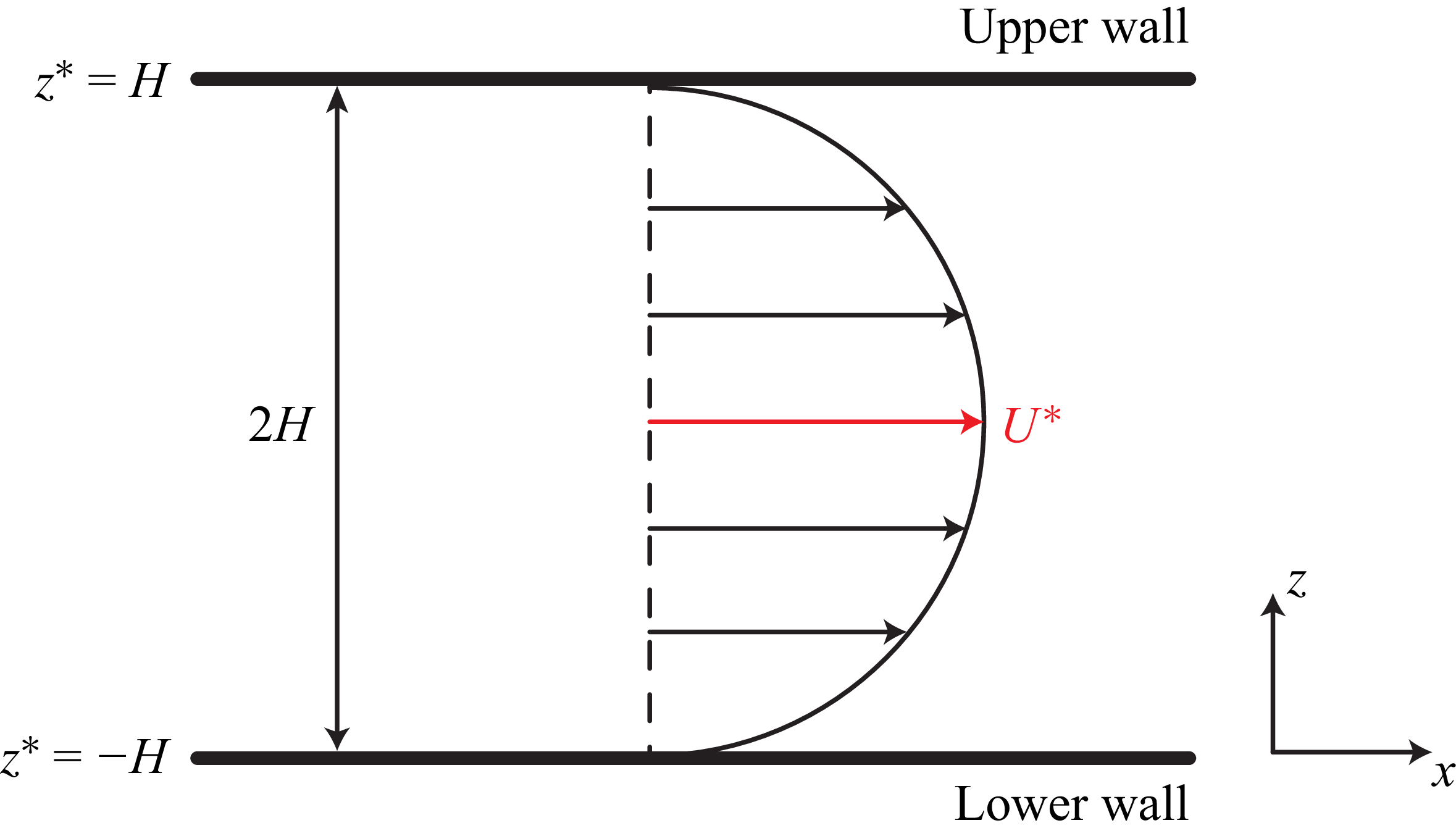

 Re=50
 β=0.98
 Re=800
 β=0.8
 Ri=0
 Ri=0.74
 Ra=−1.036×10⁵
 Ri=0.25
 Ra=−8.96×10⁶
 (Ri,W)=(−0.8,0)
 (Ri,W)=(−0.8,10)
 (Ri,W)=(−0.8,25)
 (Ri,W)=(−0.5,25)
 (Ri,W)=(−0.2,250)
 (Ri,W)=(0.2,250)

 u~
 w~
 ρ~
 τ~xx
 u~
 w~
 ρ~
 τ~xx

 ωi
 W
 Ri
 Re=50
 β=0.98
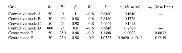
 ωi
 Sc=1000

 Epke
 Nu
 tr(τ)
 Epke
 2ωi
 tr(τ)
 tr(τ)−[[tr(τ)]]z
 [[(⋅)]]z

 Epke
 Nu
 w′
 tr(τ)
 Nu
 Epke
 2ωi

 ⟨Nu⟩
 Re
 W
 ⟨Nu⟩
 Re
 W
 β=0.98
 Ri=−0.8
 W=12.5
 ⟨Nu⟩
 Re
 Sc
 β=0.98,Ri=−0.8
 W=12.5

 β=0.98
 Ri=−0.8
 ⟨Nu⟩
 cp
 u¯(z)
 U0=1−z2
 Nu
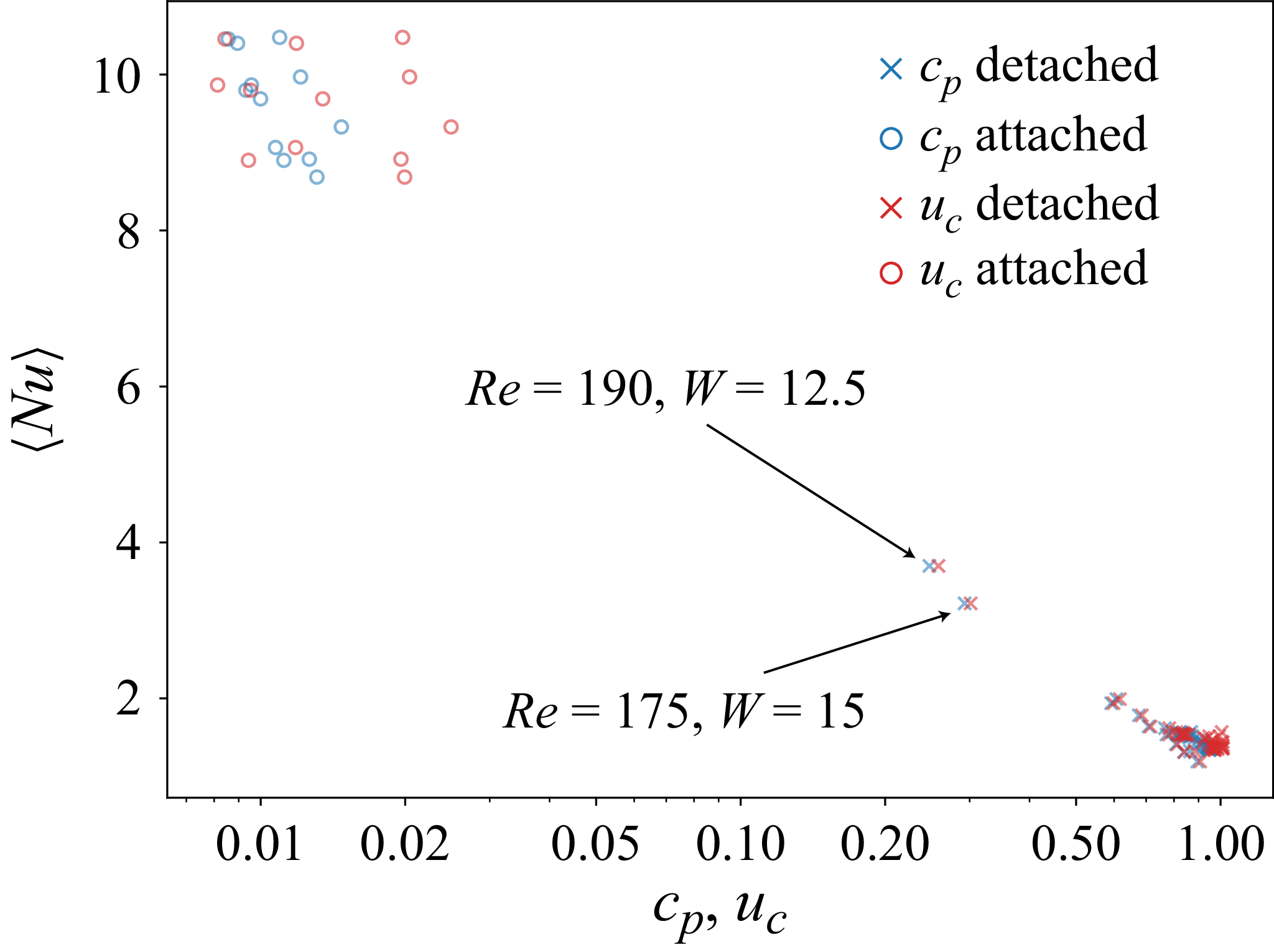
 ⟨Nu⟩
 cp
 uc

 Re=200,W=12.5,β=0.98
 Ri=−0.8
 tr(τ)
 t=0,200,400
 Ubulk
 Nu
 max[tr(τ)¯]

 T/B
 ⟨Nu⟩

 T
 ⟨Nu⟩
 W
 Re=100
 β=0.98
 Ri=−0.8
 T
 ⟨Nu⟩
 Nu
 ⟨Nu⟩=1
 T
 W
 W≥50
 T=13.8W−249.8

 Δθ∗=50∘C
 κ=1.43×10⁻⁷
 m2s−1
 α=2×10⁻⁴
 K−1
 ν=10−6
 m2s−1
 g=9.8
 ms−2

 η
 St
 Re
 W

 ⟨Nu⟩
 Re
 W
 β=0.98
 Ri=−0.8
 Tf/Bf
 Tp/Bp

 Open access

