2.1. Initial configurations

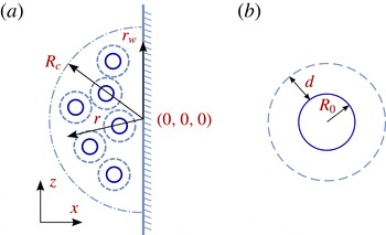
The 50 initially spherical bubbles, each of radius $R_{0}=0.3~\text{mm}$ , are positioned randomly next to the wall at $x=0$ , each fully within a hemisphere of radius $R_{c}=7.37~\text{mm}$ centred at $(0,\,0,\,0)$ and subject to the constraint that the initial separation between the surfaces of any two bubbles is greater than $2d=1.4~\text{mm}$ (figure 1). The minimum distance between a bubble surface and the wall is also $d$ , so we do not consider cases in which the bubbles sit directly on the wall, though this might be an important factor in damage in some cases. Polydispersity can also be an important factor (Wang Reference Wang1999; Shimada, Matsumoto & Kobayashi Reference Shimada, Matsumoto and Kobayashi2000; Ando et al. Reference Ando, Colonius and Brennen2011), which we do not consider in these idealized models.

Figure 1.

Schematic of (a) a random but non-overlapping arrangement of bubbles of radius $R_{0}$ within the hemisphere of radius $R_{c}$ , and (b) a representative bubble with the exclusion constraint $d$ .

The bubble sizes in our simulations are similar to those seen in similar experimental studies, such as those of Kameda & Matsumoto (Reference Kameda and Matsumoto1996) and Kameda et al. (Reference Kameda, Shimaura, Higashino and Matsumoto1998), and the initial inter-bubble spacings are selected to give a relatively low initial gas volume fraction ( $6.5\times 10^{-3}$ ), such as is also observed (Kameda & Matsumoto Reference Kameda and Matsumoto1996; Kameda et al. Reference Kameda, Shimaura, Higashino and Matsumoto1998; Bremond et al. Reference Bremond, Arora, Ohl and Lohse2006; Arora, Ohl & Lohse Reference Arora, Ohl and Lohse2007). However, the number of bubbles represented is considerably smaller owing to computational cost. The 50 bubbles simulated reflect a compromise between accounting for detailed bubble–bubble interactions of the kind expected in an actual cloud and keeping the computational cost manageable with available computational resources.

To generate this configuration, bubbles were sequentially added at random positions in this hemisphere subject to the separation constraint. The entire simulation domain in Cartesian coordinate spanned $(x,\,y,\,z)\in [-30,\,0]\times [-30,\,30]\times [-30,\,30]~\text{mm}^{3}$ . One-dimensional characteristic boundary conditions are used to model an infinite fluid-filled domain beyond the simulation domain.

All initial velocities are zero though motion starts immediately due to the initial pressure $p_{g}>p_{\infty }$ in the bubbles, where $p_{\infty }=0.1~\text{MPa}$ is the ambient pressure. The initial pressure is uniform within each bubble and decays smoothly into the liquid with a hyperbolic tangent profile $\tanh [(r_{i}-R_{0})/(R_{0}+d)]$ , where $r_{i}$ is the distance of a point in the domain from the centre of the nearest bubble $i$ . We use this mollified pressure field to prevent sharp pressure jumps at the bubble surfaces and the resulting emission of spurious compression waves. It decays within the initial bubble separation distance $2(R_{0}+d)$ and thus provides a better characterized initial condition than, say, a $1/r$ pressure decay by removing bubble–bubble pressure interaction from the initial condition. We shall see that the pressure due to the bubble dynamics quickly overwhelms this initial smooth distribution. The liquid is water with initial density ${\it\rho}_{l,0}=1000~\text{kg}~\text{m}^{-3}$ . The initial gas density ${\it\rho}_{g,0}$ is obtained from the barotropic relation $p_{g}/p_{\infty }=({\it\rho}_{g,0}/{\it\rho}_{\infty })^{{\it\gamma}_{g}}$ , with ${\it\rho}_{\infty }=1~\text{kg}~\text{m}^{-3}$ , and ${\it\gamma}_{g}=1.4$ .

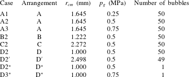
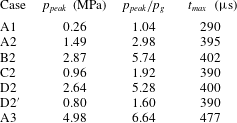
Initial bubble over-pressure ratios are $p_{g}/p_{\infty }=2.5$ , 5, and 7.5, and we consider four different random arrangements (A, B, C, and D) as summarized in table 1. These initial over-pressures are sufficiently strong to cause violent collapses, but more intense pressures are expected in some applications (Brujan et al. Reference Brujan, Ikeda, Yoshinaka and Matsumoto2011, Reference Brujan, Ikeda and Matsumoto2012). We limit our simulations to these pressures to facilitate numerical convergence for our observables. The specific bubble locations are tabulated in supplementary data available at http://dx.doi.org/10.1017/jfm.2015.287, tables S1 and S2. Case D2 is a variant of arrangement D, in which the centremost bubble is placed at $x=R_{0}+d=1~\text{mm}$ and $y=z=0$ . Throughout the paper, we refer to the centremost bubble as the bubble closest to the coordinate system origin, near the wall, not the bubble closest to the geometrical centre of the cluster. Similarly, arrangement $\text{D}^{\prime }$ is derived from D by removing this centremost bubble, and arrangement $\text{D}^{\ast }$ is a single-bubble case with only the centremost bubble of D.

Table 1.

Cases simulated, with $r_{cm}$ the initial radial location of the centremost bubble and $p_{g}$ the initial bubble pressure.

The liquid is water, which is modelled with a stiffened equation of state (Menikoff & Plohr Reference Menikoff and Plohr1989), and the gas inside the bubbles is air modelled as ideal; the equation of state parameters are those of Saurel & Abgrall (Reference Saurel and Abgrall1999b ). Based on $R_{0}$ , the characteristic speed $\sqrt{p_{g}/{\it\rho}_{l,0}}$ , and water-like kinematic viscosity ${\it\nu}=10^{-6}~\text{m}^{2}~\text{s}^{-1}$ , the Reynolds numbers range from $\mathit{Re}=4743$ to 8216, which justifies neglecting viscosity in the simulations. The corresponding Weber numbers for an air–water surface tension $0.07~\text{N}~\text{m}^{-1}$ range from 1071 to 3214, which similarly justifies neglect of surface tension. Though in some cases surface tension and viscosity can influence some details of jetting and fragmentation during the final stages of a bubble collapse (Popinet & Zaleski Reference Popinet and Zaleski1999, Reference Popinet and Zaleski2002), we neglect those effects to focus on bubble–bubble interactions in this study. Similarly, thermal and mass diffusion are neglected, as is phase change, though it has been considered in some other studies (Esmaeeli & Tryggvason Reference Esmaeeli and Tryggvason2004a ,Reference Esmaeeli and Tryggvason b ; Hardt & Wondra Reference Hardt and Wondra2008; Lauer et al. Reference Lauer, Hu, Hickel and Adams2012). For the current conditions, the liquid pressure remains above the saturation pressure at room temperature.

2.2. Numerical methods

Full details of the numerical scheme along with detailed convergence studies and comparisons with semi-analytic solutions are reported in our previous paper (Tiwari, Freund & Pantano Reference Tiwari, Freund and Pantano2013), and are thus only summarized here. The gas–liquid description is based upon a variant of the Baer–Nunziato model (Baer & Nunziato Reference Baer and Nunziato1986) by Saurel & Abgrall (Reference Saurel and Abgrall1999a ), which uses a mixture description to represent the phases without any explicit Lagrangian tracking of the interface. The interfaces are thus thin mixture regions represented on a fixed mesh. These interfaces are maintained thin via thermodynamically consistent localized ‘sharpening’ terms added to the governing equations (Tiwari et al. Reference Tiwari, Freund and Pantano2013):

where the gradient of gas mass fraction, $\boldsymbol{{\rm\nabla}}({\it\rho}_{g}{\it\alpha}_{g})$ , localizes its action to the interface in the corresponding transport equation

In (2.1), $\mathscr{U}_{0}$ is a sharpening strength, $\boldsymbol{n}$ is the interface normal, and ${\it\epsilon}\approx 1.5{\rm\Delta}x_{min}$ , where ${\rm\Delta}x_{min}$ is the refined mesh spacing (discussed subsequently). This ${\it\epsilon}$ factor thus restricts the thickness of the interface. The remaining parameters are the gas density ${\it\rho}_{g}$ , the mixture velocity $\boldsymbol{u}$ , the gas volume fraction ${\it\alpha}_{g}$ , and the liquid volume fraction ${\it\alpha}_{l}$ . The corresponding $\mathscr{R}$ -like terms in the other transport equations are designed to be thermodynamically consistent with the same mixture law, in order for the thermodynamic state to remain collectively consistent within the thin mixture region (Tiwari et al. Reference Tiwari, Freund and Pantano2013). This avoids the spurious oscillations that can occur for sharp interfaces when thermodynamic consistency is not respected within the thin interface zone. It also allows interfaces to be always sufficiently resolved by the underlying mesh.

The compressible-flow equations that represent both fluids are discretized on a fixed Cartesian mesh, and are solved using a finite-volume description based upon the common reconstruct-evolve-average approach (Toro Reference Toro2006). A total variation diminishing third-order Runge–Kutta method (Gottlieb & Shu Reference Gottlieb and Shu1988) is used for time integration. The necessary Riemann problems are solved approximately using the HLLC method (Johnsen & Colonius Reference Johnsen and Colonius2006; Toro Reference Toro2006). A fifth-order WENO scheme (Jiang & Shu Reference Jiang and Shu1996; Titarev & Toro Reference Titarev and Toro2004) is employed for spatial reconstruction.

The algorithm is implemented in an adaptive mesh refinement (AMR) (Deiterding et al. Reference Deiterding, Radovitzky, Mauch, Noels, Cummings and Meiron2006) framework per the specifications discussed in the following subsection. A typical simulation used four levels of adaptive refinement, which corresponds to about $2\times 10^{7}$ computational cells for the initial configurations. This same local resolution would require about $2\times 10^{9}$ uniformly distributed mesh points for the domain studied. The total cost of a typical simulation presented here is 144 h on 120 cores with the Intel HP X5650 2.66 GHz 6C processor.

2.3. Resolution assessment

The numerical algorithm has been validated extensively against many test problems, including single-bubble collapses, in our previous paper (Tiwari et al. Reference Tiwari, Freund and Pantano2013). There, we reported excellent agreement between our detailed three-dimensional single-bubble simulations and highly accurate spherically symmetric Keller–Miksis solutions. Here we only confirm resolution sufficiency for the present configurations. The simulations discussed in § 3 used a minimum AMR mesh spacing ${\rm\Delta}x_{min}=39~{\rm\mu}\text{m}$ , which corresponds to $n=R_{0}/{\rm\Delta}x_{min}=7.7$ cells per initial bubble radius. 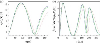We first performed a detailed resolution study on the single-bubble case $\text{D}3^{\ast }$ (table 1). Figure 2 shows the convergence of gas volume and total kinetic energy history with grid refinement. The effect of resolution on actual cluster simulation is discussed further in the next section.

Figure 2.

(a) Gas volume history, and (b) total kinetic energy for case $\text{D}3^{\ast }$ at different resolutions $n$ : $\cdots \cdots$ , $n=3.8$ ; ——, $n=7.7$ ; – – –,  $n=15.4$ .

3.1. Overall cluster dynamics

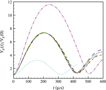
The cluster gas volume histories $V_{g}(t)$ for the 50-bubble cases are shown in figure 3, including a confirmation of mesh independence for case D2. The effect of initial pressure is obvious. Higher initial pressures (case A3) lead to larger expansion of the bubbles and longer times to collapse; lower initial pressures (case A1) do the opposite.

Figure 3.

Gas volume history: $\cdots \cdots$ , A1; - - - -, A2; – – –, B2; — — —, C2; — —, D2; — ⋅ —, A3 listed in table 1; and ——, D2 at double resolution ( $n=15.6$ ).

For fixed initial pressure but different random bubble distributions, the gas volume history for all four $p_{g}/p_{\infty }=5$ cases (A2, B2, C2, and D2) are similar. This suggests that our cluster is sufficiently large that the particular dynamics of the random arrangements approximately average out and do not affect much this global quantity. A well-crafted homogenization might therefore be evaluated for reproducing this behaviour. However, despite the similarities of the overall collapse, there is a factor-of-three case-to-case difference in the peak pressures within the cluster (table 2). (Doubling the resolution to $n=15.6$ for case D2 leads to a pointwise variation of less than 7 % in peak pressure, which is far less than the arrangement-to-arrangement variability.) We also note that for all the cases considered, the peak pressures exceed the initial overpressure ( $p_{peak}/p_{g}>1$ ). For the expansion and collapse of an isolated single bubble in a free field, the Keller–Miksis model (Keller & Miksis Reference Keller and Miksis1980) gives $p_{peak}=0.24$ , 0.46, and 0.67 MPa for $p_{g}=0.25$ , 0.5, and 0.75 MPa, respectively, implying $p_{peak}/p_{g}<1$ . Thus, we can already conclude that bubble–bubble interactions promote some form of pressure amplification. The specific interactions leading to this are discussed in the following subsection.

Table 2.

$p_{peak}$ and $t_{max}$ for different initial arrangements.

3.2. Detailed bubble dynamics

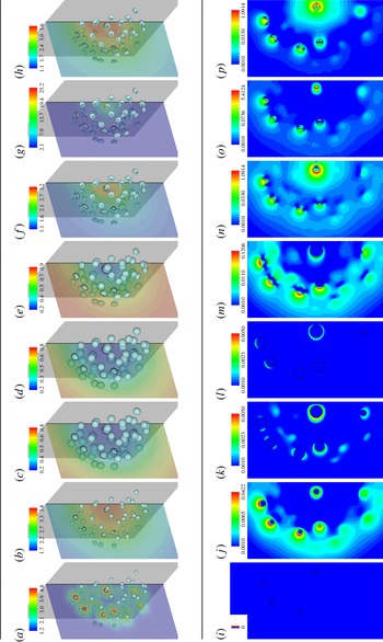
Figure 4 shows the entire expansion and collapse of the D2 cluster. The initial mollified pressure and the corresponding zero-velocity initial condition at $t=0~{\rm\mu}\text{s}$ are seen in figures 4(a) and 4(i). By $t=20~{\rm\mu}\text{s}$ , all the bubbles are obviously expanding, with a nearly uniform high pressure spanning the cluster (4 b). However, the kinetic energy (4 j) shows that the bubbles toward the centre of the cluster are expanding relatively slowly or not at all. This delay is due to the collective focusing of a compression wave generated by each over-pressured bubble of the initial condition. The outermost bubbles, which at this time are exposed to the lower ambient pressure, are the least confined by this compression. This trend reverses by $t=170~{\rm\mu}\text{s}$ , when a relatively low pressure now spans the core (4 c) and drives a delayed expansion of the inner bubbles (4 k). As was seen in figure 3, by $t=200~{\rm\mu}\text{s}$ the cluster is near its maximum overall volume, though not all bubbles are in phase with this overall behaviour. At this time, the inner bubbles are still expanding in a low-pressure region (4 d) while the outer bubbles have begun to collapse, as seen by their kinetic energy and deforming shapes (4 l).

Figure 4.

(a–h) Bubble shapes and pressure contours and (i–p) kinetic energy contours for case D2 in table 1. Note logarithmic scale for kinetic energy contours. (a,i) $t=0~{\rm\mu}\text{s}$ , (b,j) $t=20~{\rm\mu}\text{s}$ , (c,k) $t=170~{\rm\mu}\text{s}$ , (d,l) $t=200~{\rm\mu}\text{s}$ , (e,m) $t=320~{\rm\mu}\text{s}$ , (f,n) $t=390~{\rm\mu}\text{s}$ , (g,o) $t=400~{\rm\mu}\text{s}$ , (h,p) $t=410~{\rm\mu}\text{s}$ .

We note that despite the nearly spherical bubble shape in the expansion phase up to $t=200~{\rm\mu}\text{s}$ in figure 4(d), the non-uniform pressure field sets the directionality and potentially initiates the jetting during the collapse phase. At this time, we also see bubble shapes consistent with the onset of jetting behaviour. These and subsequent frames in the visualized time series show that the collapse starts in the outer regions.

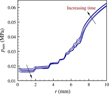
The evolution of the pressure around $t=200~{\rm\mu}\text{s}$ is further quantified in figure 5, which shows minimum pressure $p_{min}$ versus the radial distance $r$ . We see that $p_{min}$ is decreasing from $t=200$ to $240~{\rm\mu}\text{s}$ near the central region while increasing in the outer region, which confirms that the central bubbles are still expanding while the outer bubbles have begun to collapse.

Figure 5.

The pressure minima $p_{min}(r)$ for case D2 versus the radial distance $r$ from the cluster centre (shown in figure 1 a) for times $t=200{-}240~{\rm\mu}\text{s}$ , showing the transition from expansion to collapse. Equal time intervals are shown with increasing  $t$ .

By $t=320~{\rm\mu}\text{s}$ , kinetic energy suggests a strong jetting toward the cluster centre (figure 4 m), which is confirmed by the corresponding visualizations of velocity (not shown). However, at this same time the centremost bubble retains a much larger volume, and is still in a relatively low-pressure region (4 e). This is reversed by $t=390~{\rm\mu}\text{s}$ (figure 4 f,n), when the collapse has reached the centremost bubble with an apparent focusing of kinetic energy and pressure associated with the inward progress of collapse. The highest kinetic energy is now tightly focused on the side of the centremost bubble that is furthest from the wall. Just $10~{\rm\mu}\text{s}$ later at $t=400~{\rm\mu}\text{s}$ , this bubble is almost fully collapsed (4 g and 4 o), which is followed by a fast re-expansion by $t=410~{\rm\mu}\text{s}$ (4 h and 4 p). We note from figure 3 that the onset of re-expansion occurs when the overall gas volume is still decreasing. Liquid inertia generates very high pressure in the centremost bubble in a short time, which drives its rapid re-expansion. Peak pressure in the domain is generated during the fast collapse and re-expansion of the centremost bubble just before the overall cluster attains minimum bubble volume. Table 2 and figure 3 show a similar trend for all the cases considered.

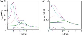
The pressure field at the time of overall peak pressure is quantified in figure 6, where we plot the maximum pressure $p_{max}$ versus the radial distance $r$ and on the wall for cases A2 to D2, which have the same initial over-pressure in the bubbles (table 1). For all cases, the peak pressure is associated with the centremost bubble, the location of which is also shown schematically in the figure. This is the case in the bulk fluid and for the wall pressures. Visualization of the wall pressures in figure 7 show that it is relatively simple and axisymmetric despite the complexity of the bubble dynamics. The same is true for case $\text{D}2^{\prime }$ , which is equivalent to case D2 though with the centremost bubble removed. The peak pressure is now obviously associated with the next-to-centremost bubble at $r_{cm}=2.50~\text{mm}$ for D2, now filling the role of the centremost bubble for $\text{D}2^{\prime }$ .

Figure 6.

The pressure maxima at the time when peak pressure is observed for cases $\cdots \cdots$ , A2; — ⋅ —, B2; – – –, C2; — ⋅ ⋅ —, D2; ——, $\text{D}2^{\prime }$ : (a) versus the radial distance $r$ from the cluster centre, and (b) along the wall at radius $r_{w}$ from the centre of the cluster. Circles indicate the radial location of the centremost bubble.

Figure 7.

Wall pressure at the instant of peak wall pressures. Note the logarithmic colour scale, with units of pressure $\times 10^{5}~\text{Pa}$ . (a) A2, (b) B2, (c) C2, (d) D2.

The collapse of the centremost bubble for cases A2 to D2 is visualized in detail in figure 8, which shows momentum vectors ${\it\rho}\boldsymbol{u}$ at $t=400~{\rm\mu}\text{s}$ projected onto the plane that intersects both the centre of the centremost bubble and the axis of symmetry of the hemisphere that defines the bubble cluster (see figure 1 a). Here we see the asymmetrical bubble dynamics, particularly the re-entrant jetting. The specific environment in the cluster of the centremost bubble determines the details of this jetting and thereby the actual peak pressures and potential for wall damage. It is clear in figure 8 that these bubbles collapse differently in different cases. This variation would be anticipated to give rise to significant collapse-to-collapse variability in damage to adjacent material, though thorough investigation of that is beyond the scope of this study.

Figure 8.

Momentum vectors along the plane normal to the $x{-}y$ plane containing the centre of the hemisphere and the centre of the centremost bubble at $t=400~{\rm\mu}\text{s}$ for: (a) A2, (b) B2, (c) C2, (d) D2.

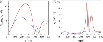
To quantify the kinetic energy associated with the non-spherical deformations, we consider the centremost and, for contrast, outermost bubbles of case A2. The gas volume histories $V_{g,i}(t)$ for these two bubbles are shown in figure 9(a). We note that the volume of the centremost bubble has a maximum near $270~{\rm\mu}\text{s}$ and local minima near 400 and $460~{\rm\mu}\text{s}$ , while the outermost bubble has a maximum near $180~{\rm\mu}\text{s}$ and a minimum near $430~{\rm\mu}\text{s}$ . We now define a region surrounding a bubble in which we compute the mass-specific non-translational average kinetic energy ${\it\kappa}_{i}(t)$ of the liquid. This region is a sphere concentric with the bubble’s centre of mass, and its radius is such that it encloses a fixed liquid mass $m_{0}$ :

We use the initial liquid density ${\it\rho}_{l,0}$ and initial bubble radius $R_{0}$ to define this fixed mass:

The average kinetic energy ${\it\kappa}_{i}(t)$ is then

where $\boldsymbol{u}$ is the velocity and $\bar{\boldsymbol{u}}$ is the average velocity in the spherical region,

which we subtract from the velocity in (3.3) to remove the translational component of velocity.

Figure 9.

(a) Gas volume histories and (b) mass specific kinetic energy of the liquid surrounding the bubbles: ——, centremost; – – –, outermost.

The kinetic energy histories for the two bubbles are shown in figure 9(b). We observe that the kinetic energies increase initially due to the initial acceleration of the bubbles. They reach local maximum, then reduce, and nearly vanish near maximum gas volume. This is consistent with the spherical bubble shapes observed in figure 4 during the expansion phase: if the bubbles remain spherical then kinetic energy must vanish when the gas volume attains local maximum or minimum. After this, the kinetic energies again increase during the collapse phase, and we note that kinetic energies do not vanish at the subsequent local minima or maxima. This is again consistent with the non-spherical bubble shapes and the kinetic energy contours observed in figure 4 during the collapse phase, and the momentum vectors observed in figure 8. This is clearly indicative of the loss in energy to the liquid jets, which leads to the weaker rebound of the bubbles observed in figure 9(a).

Based on the gas volume history in figure 3, we note that though the central bubbles undergo relatively stronger collapses, the over-pressures in our simulations are such that the average strength of bubble collapse is relatively weak (Philipp & Lauterborn Reference Philipp and Lauterborn1998; Lindau & Lauterborn Reference Lindau and Lauterborn2003). In this weak-strength but strong-interaction regime, the energy lost to re-entrant jetting is higher than viscous, thermal, and acoustic damping mechanisms. This was anticipated by Brennen (Reference Brennen2002), who suggested that more kinetic energy might be lost in bubble fragmentation than all other damping mechanisms. Similarly, Delale & Tunc (Reference Delale and Tunc2004) developed a modified Rayleigh–Plesset model to account for fission losses during rebound. The other mechanisms are expected to become relatively more important in more intense collapses (Fuster, Dopazo & Hauke Reference Fuster, Dopazo and Hauke2011), particularly for vapour-filled cavities (Akhatov et al. Reference Akhatov, Lindau, Topolnikov, Mettin, Vakhitova and Lauterborn2001). In strong collapses of relatively weakly interacting bubbles, they would behave more as individual units, and the energy loss to kinetic energy via jetting or similar mechanisms could be much smaller compared to the dominant damping for spherical collapses. Quantifying in detail any switch-over of the dominant damping mechanisms would require more challenging simulations of more violent bubble collapses.

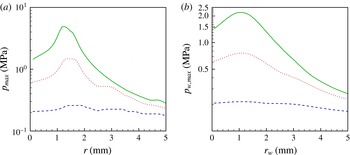
We now consider the dependence upon initial overpressure, examining cases A1 to A3 from table 1 with pressure ratios $p_{g}/p_{\infty }=2.5$ , 5.0, and 7.5. The gas volume histories in figure 3 suggest that the high pressure will lead to both larger volumes of individual bubbles and bubble surfaces that more closely interact. Therefore, we anticipate both more violent dynamics associated with individual bubbles and stronger bubble–bubble interactions. The peak pressures generated during the final stage of the collapse bear this out (table 2). For comparison, we list the ratio of the peak pressure generated to the initial over-pressure in the bubbles $p_{peak}/p_{g}$ . 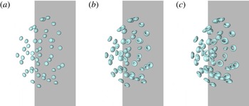Almost no pressure amplification is observed for the case A1 ( $p_{g}/p_{\infty }=2.5$ ), which suggests that the bubbles in this case behave approximately independently. Indeed, corresponding visualizations suggest that the bubbles remain roughly spherical (figure 11). However, interactions become pronounced with increasing initial over-pressure for cases A2 and A3, suggesting that collective bubble behaviour dominates at these large initial over-pressures. The peak pressure at radius $r$ shown in figure 10 is nearly flat for case A1 ( $p_{g}/p_{\infty }=2.5$ ) but increases significantly for A3 ( $p_{g}/p_{\infty }=7.5$ ) and is obviously associated with the radial location of the centremost bubble.

Figure 10.

The pressure maxima $p_{max}(r,\,t)$ at the time when peak pressure is observed for cases – – –, A1; $\cdots \cdots$ , A2; ——, A3: (a) versus the radial distance $r$ from the cluster centre and (b) along the wall at radius $r_{w}$ from the centre of the cluster.

Figure 11.

Bubble shapes near the minimum volume for cases (a) A1, $t=300~{\rm\mu}\text{s}$ ; (b) A2, $t=400~{\rm\mu}\text{s}$ ; (c) A3, $t=480~{\rm\mu}\text{s}$ .

4.1. Homogeneous-mixture model

The homogeneous-mixture barotropic model we consider, like many such models that have been employed, is based on two main assumptions (van Wijngaarden Reference van Wijngaarden1972; Brennen Reference Brennen1995): (i) both the bubble sizes and the inter-bubble spacings are small relative to the pressure variation scale (wavelength) in the surrounding flow field, and (ii) the natural frequencies of the bubbles are large relative to the time scales of the overall flow field. The resulting mixture mass and momentum equations are similar to those for single-phase flows (van Wijngaarden Reference van Wijngaarden1972; Brennen Reference Brennen1995):

where ${\it\rho}$ is the mixture density, $p$ is the mixture pressure and $\boldsymbol{u}$ is the mixture velocity. A suitable barotropic relation completes the system. For isentropic flows without mass transfer, this is (Brennen Reference Brennen1995)

where ${\it\alpha}_{1,2}$ , $s_{1,2}$ and ${\it\rho}_{1,2}$ are respectively the volume fractions, entropies, and densities of the respective phases, and $s$ is the mixture entropy. The stiffened equation of state we use (Menikoff & Plohr Reference Menikoff and Plohr1989) gives

and thus

where $p_{k}^{\infty }$ and ${\it\gamma}_{k}$ are the stiffened gas equation of state parameters of phase $k=1,\,2$ . This state equation models the physics of the molecular attraction in the liquid as if it were an ideal gas pre-compressed with pressure $p^{\infty }$ , which thus serves as a model parameter. Following Saurel & Abgrall (Reference Saurel and Abgrall1999b ), we take $p_{1}^{\infty }=600~\text{MPa}$ to model liquid water, for which the polytropic exponent ${\it\gamma}_{1}=4.4$ produces the correct speed of sound. For the gas phase, we take $p_{2}^{\infty }=0$ and ${\it\gamma}_{2}=1.4$ . Together (4.2) and (4.3) provide a mixture pressure–density relation,

from which $p({\it\rho})$ closes (4.1).

To facilitate comparison, we specify an initial condition to match that of the detailed simulation. In doing this, most quantities are straightforward to select. The initial gas volume fraction ${\it\alpha}_{0}$ and initial density ${\it\rho}_{0}$ of the homogeneous mixture are obtained by averaging, and the initial momentum is zero in both configurations. However, specifying the initial pressure (or, equivalently, mixture energy) is not straightforward. Setting a uniform pressure by averaging that of the detailed configuration does not conserve energy between the two configurations. Likewise, forcing conservation of total initial internal energy unphysically redistributes it between the liquid and gas in a way that disrupts the momentum balance between the two configurations (Brennen Reference Brennen1995).

To avoid ambiguity in the initial condition, we run new bubble-detailed simulations with an equivalent initial condition to facilitate correspondence. The bubbles and liquid in the cluster hemisphere are given a uniform over-pressure $p_{g}$ . Beyond the cluster, the pressure decays smoothly to $p_{\infty }$ with the same hyperbolic tangent profile used in § 2. The arrangement matches the A configuration from table 1 and the parameters match that of case A2. The same uniform pressure is unambiguously used in the homogeneous-mixture model.

The same numerical solver is used for the homogeneous mixture, though without the interface correction terms (Tiwari et al. Reference Tiwari, Freund and Pantano2013), so the region fills the entire hemisphere. The other simulation conditions for the homogeneous-fluid configuration match those for the detailed configuration.

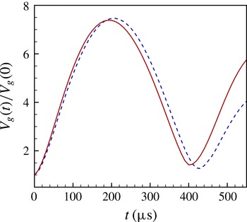
Figure 12 shows that the homogeneous-mixture model provides a qualitatively correct and reasonably accurate prediction of the overall gas volume history compared to the bubble-detailed simulation, especially up to the minimum-volume collapse point. After this point, it starts to deviate further, since the complexity of the actual bubble dynamics in the collapse cannot be reproduced by the model.

Figure 12.

Gas volume history using: ——, the homogeneous-mixture model; – – –, the detailed simulation.

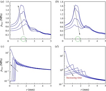
The radial pressure profiles for the detailed simulation during the final stage of the collapse are shown in figure 13(a,b). They are similar to the cases discussed in § 3, with peak pressure generation near the centremost bubble. In contrast, the corresponding profiles for the homogeneous-fluid model shown in figure 13(c,d) show that its collapse includes a strong compression wave that focuses to form a very high peak impulsive pressure ( ${>}23~\text{MPa}$ ). The inward propagation and reflection from the wall of these waves is shown in figure 13(c). The re-expansion is also qualitatively different.

Figure 13.

(a,b) Detailed simulations: $p_{max}$ versus $r$ for time ranges (a)  $t=391{-}397~{\rm\mu}\text{s}$ , (b)  $t=397{-}403~{\rm\mu}\text{s}$ , for the special detailed simulation considered in this section. (c,d) Pressure $p$ along the homogeneous-mixture radius $r$ for times (c) $t=367.5{-}371.5~{\rm\mu}\text{s}$ , (d)  $t=371.5{-}375.5~{\rm\mu}\text{s}$ .

We thus conclude this section by noting that the pressure distributions obtained from the simplified model are fundamentally different throughout the simulation, which makes the volume history predicted by this same model seem surprisingly good.

4.2. Bubble–particle models

Particle-based models assume simple bubble dynamics but do not assume that cluster-scale pressure interactions are smooth (Parlitz et al. Reference Parlitz, Mettin, Luther, Akhatov, Voss and Lauterborn1999; Doinikov Reference Doinikov2004; Yasui et al. Reference Yasui, Iida, Tuziuti, Kozuka and Towata2008; Lauterborn & Kurz Reference Lauterborn and Kurz2010; Zeravcic, Lohse & Van Saarloos Reference Zeravcic, Lohse and Van Saarloos2011). In the basic approach, the $N$ bubbles comprising the cloud are assumed spherical with radii governed by coupled Rayleigh–Plesset-like equations augmented to account for weak bubble–bubble interactions (Mettin et al. Reference Mettin, Akhatov, Parlitz, Ohl and Lauterborn1997; Pelekasis et al. Reference Pelekasis, Gaki, Doinikov and Tsamopoulos2004). The cluster model we use here for comparison is an extension of the two-bubble Keller–Miksis-like model presented in Mettin et al. (Reference Mettin, Akhatov, Parlitz, Ohl and Lauterborn1997); it is similar to other cluster models (Doinikov Reference Doinikov2004; Bremond et al. Reference Bremond, Arora, Ohl and Lohse2006; Yasui et al. Reference Yasui, Iida, Tuziuti, Kozuka and Towata2008):

where $R_{i}$ and $p_{b,i}$ are the radius and pressure of bubble $i$ , $d_{ij}$ is the separation distance between bubbles $i$ and $j$ , ${\it\rho}_{1}$ is the liquid density, $p_{\infty }$ is the pressure in the liquid far away from the bubbles, and $a_{1}$ is the speed of sound in the liquid. The summation over all the particle-like bubbles accounts for the leading-order ${\sim}R_{j}/r$ component of the pressure field induced by other bubbles; higher-order pressure components, translation of the bubbles, and higher-order liquid compressibility effects are neglected, although they could be included in principle (Doinikov Reference Doinikov2004; Ilinskii, Hamilton & Zabolotskaya Reference Ilinskii, Hamilton and Zabolotskaya2007; Fuster & Colonius Reference Fuster and Colonius2011) and some comparisons are available (Fuster et al. Reference Fuster, Dopazo and Hauke2011). Bremond et al. (Reference Bremond, Arora, Ohl and Lohse2006) employed a similar model to describe the expansion and collapse of a regular array of 37 bubbles. In that organized configuration, the bubble radii predicted by the model agreed well with their experimental study, except during the collapse phase when the bubbles are obviously non-spherical due to the re-entrant jetting toward the cluster centre. The wall in our configuration acts as a symmetry plane and thus is incorporated in (4.6) via the method of images.

Equation (4.6) is solved for all the cases, with initial radii $R_{i}(0)=R_{0}=0.3~\text{mm}$ , and initial velocities $\dot{R_{i}}(0)=0$ . 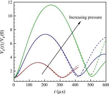However, to account for the different initial pressure field assumed in the reduced model compared to the detailed simulation, the initial bubble pressures $p_{b,i}(0)$ are not set to the initial pressure $p_{g}$ in the detailed simulation; they are set to an adjusted pressure $\tilde{p}_{g}$ , which is obtained such that the maximum gas volume attained in the particle model matches that in the corresponding detailed simulation. We see in figure 14 that the gas volume histories obtained from the reduced model are close to the detailed simulations up to the collapse. Since the bubbles largely remain spherical during the expansion (§ 3), the model is expected to be most successful during this phase. However, as seen in § 3, the bubbles are increasingly aspherical as the collapse propagates inward. Consequently, the reduced model increasingly becomes less accurate and deviates more from the detailed simulations during the cluster collapse, especially after the rebound.

Figure 14.

Gas volume histories for cases A1 to A3 obtained from: ——, detailed simulations; – – –, the reduced model.

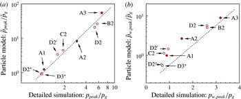
Though the gas volume histories are accurate, peak pressures are significantly different. This is shown in figure 15, where we compare the peak pressures during the final stage of the collapse for the reduced model and detailed simulations. The disagreement increases significantly at higher initial bubble pressures. We see that the particle model overpredicts the peak pressures by nearly a factor of 10 in these most violent cases, when the aspherical dynamics of the bubbles were observed to be most pronounced in § 3. The corresponding pressures on the wall follow essentially the same trend as the bulk pressures. There is a clear trend to this overprediction with increasing pressures, which is consistent with the discussion in § 3.2. Stronger interactions result in more bubble energy becoming focused into the re-entrant jets and therefore not recoverable for bubble re-expansion. Thus, asymmetric collapses mollify the spherical-bubble peak pressures in a systematic fashion, which suggests a possible correction to predictions based on this reduced model.

Figure 15.

Comparison of peak pressure (a) in the volume and (b) on the wall obtained from detailed simulations and the particle model for cases from table 1 (○), with the common configuration A-series emphasized (●); for reference the dashed line shows $\tilde{p}_{peak}/\tilde{p}_{g}=p_{peak}^{2}/p_{g}^{2}$ in (a) and $\tilde{p}_{w,\,peak}/\tilde{p}_{g}=p_{w,\,peak}^{2}/p_{g}^{2}$ in (b).